HAL Id: hal-02969739https://hal.archives-ouvertes.fr/hal-02969739

Preprint submitted on 16 Oct 2020

HAL is a multi-disciplinary open accessarchive for the deposit and dissemination of sci-entific research documents, whether they are pub-lished or not. The documents may come fromteaching and research institutions in France orabroad, or from public or private research centers.

L’archive ouverte pluridisciplinaire HAL, estdestinée au dépôt et à la diffusion de documentsscientifiques de niveau recherche, publiés ou non,émanant des établissements d’enseignement et derecherche français ou étrangers, des laboratoirespublics ou privés.

Maxwell’s equations with hypersingularities at a conicalplasmonic tip

Anne-Sophie Bonnet-Ben Dhia, Lucas Chesnel, Mahran Rihani

To cite this version:Anne-Sophie Bonnet-Ben Dhia, Lucas Chesnel, Mahran Rihani. Maxwell’s equations with hypersin-gularities at a conical plasmonic tip. 2020. hal-02969739

Maxwell’s equations with hypersingularitiesat a conical plasmonic tip

Anne-Sophie Bonnet-Ben Dhia1, Lucas Chesnel2, Mahran Rihani1,2

1 Laboratoire Poems, CNRS/INRIA/ENSTA Paris, Institut Polytechnique de Paris, 828 Boulevarddes Marechaux, 91762 Palaiseau, France;2 INRIA/Centre de mathematiques appliquees, Ecole Polytechnique, Institut Polytechnique de Paris,Route de Saclay, 91128 Palaiseau, France.

E-mails: anne-sophie.bonnet-bendhia@ensta-paris.fr, lucas.chesnel@inria.fr,mahran.rihani@ensta-paris.fr

(October 16, 2020)

Abstract. In this work, we are interested in the analysis of time-harmonic Maxwell’s equationsin presence of a conical tip of a material with negative dielectric constants. When these constantsbelong to some critical range, the electromagnetic field exhibits strongly oscillating singularitiesat the tip which have infinite energy. Consequently Maxwell’s equations are not well-posed inthe classical L2 framework. The goal of the present work is to provide an appropriate functionalsetting for 3D Maxwell’s equations when the dielectric permittivity (but not the magnetic per-meability) takes critical values. Following what has been done for the 2D scalar case, the ideais to work in weighted Sobolev spaces, adding to the space the so-called outgoing propagatingsingularities. The analysis requires new results of scalar and vector potential representations ofsingular fields. The outgoing behaviour is selected via the limiting absorption principle.

Key words. Time-harmonic Maxwell’s equations, negative metamaterials, Kondratiev weightedSobolev spaces, T -coercivity, compact embeddings, scalar and vector potentials, limiting absorp-tion principle.

1 Introduction

For the past two decades, the scientific community has been particularly interested in the studyof Maxwell’s equations in the unusual case where the dielectric permittivity ε is a real-valuedsign-changing function. There are several motivations to this which are all related to spectacularprogress in physics. Such sign-changing ε appear for example in the field of plasmonics [3, 33, 6].The existence of surface plasmonic waves is mainly due to the fact that, at optical frequencies,some metals like silver or gold have an ε with a small imaginary part and a negative real part.Neglecting the imaginary part, at a given frequency, one is led to consider a real-valued ε whichis negative in the metal and positive in the air around the metal. A second more prospectivemotivation concerns the so-called metamaterials, whose micro-structure is designed so that theireffective electromagnetic constants may have a negative real part and a small imaginary part insome frequency ranges [46, 45, 44]. Let us emphasize that for such metamaterials not only thedielectric permittivity ε may become negative but the magnetic permeability µ as well. At theinterface between dielectrics and negative-index metamaterials, one can observe a negative refrac-tion phenomenon which opens a lot of exciting prospects. Finally let us mention that negative εalso appear in plasmas, together with strong anisotropic effects. But we want to underline a maindifference between plasmas and the previous applications. In the case of plasmonics and metama-terials, ε is sign-changing but does not vanish (and similarly for µ), while in plasmas, ε vanisheson some particular surfaces, leading to the phenomenon of hybrid resonance (see [21, 39]). The

1

theory developed in the present paper does no apply to the case where ε vanishes.

The goal of the present work is to study the Maxwell’s system in the case where ε, µ changesign but do not vanish. In case of invariance with respect to one variable, the analysis of time-harmonic Maxwell’s problem leads to consider the 2D scalar Helmholtz equation

div(1ε∇ϕ

)+ ω2µϕ = f.

Here f denotes the source term and the unknown ϕ is a component of the magnetic field. Forthis scalar equation, only the change of sign of ε matters because roughly speaking, the terminvolving µ is compact (or locally compact in freespace). In the particular case where ε takesconstant values ε+ > 0 and ε− < 0 in two subdomains separated by a a curve Σ, the results arequite complete [8]. If Σ is smooth (of class C1), the equation has the same properties in the H1

framework as in the case of positive coefficients, except when the contrast κε := ε−/ε+ takes theparticular value −1. One way to show this consists in finding an appropriate operator T suchthat the coercivity of the variational formulation is restored when testing with functions of theform Tϕ′ (instead of ϕ′). This approach is called the T-coercivity technique. When κε = −1,Fredholmness is lost in H1 but some results can be established in some weighted Sobolev spaceswhere the weight is adapted to the shape of Σ [41, 37, 42]. The picture is quite different whenΣ has corners. For instance, in the case of a polygonal curve Σ, Fredholmness in H1 is lost notonly for κε = −1 but for a whole interval of values of κε around −1. We name this interval thecritical interval. The smaller the angle of the corners, the larger the critical interval is. In fact,we can still find a solution in that case but this solution has a strongly singular behaviour atthe corners in riη where r is the distance to the corner and η is a real coefficient. In particular,this hypersingular solution does not belong to H1. It has been shown that Fredholmness can berecovered in an appropriate unusual framework [10] which is obtained by adding a singular func-tion to a Kondratiev weighted Sobolev space of regular functions. The proof requires to adaptMellin techniques in Kondratiev spaces [30] to an equation which is not elliptic due to the changeof sign of ε (see [20] for the first analysis). From a physical point of view, the singular1 functioncorresponds to a wave which propagates towards the corner, without never reaching it becauseits group velocity tends to zero with the distance to the corner [7, 25, 26]. In the literature,this wave which is trapped by the corner is commonly referred to as a black-hole wave. It leadsto a strange phenomenon of leakage of energy while only non-dissipative materials are considered.

The objective of this article is to extend this type of results to 3D Maxwell’s equations. Thecase where the contrasts in ε and µ do not take critical values has been considered in [9]. Usingthe T-coercivity technique, a Fredholm property has been proved for Maxwell equations in a clas-sical functional framework as soon as two scalar problems (one for ε and one for µ) are well-posedin H1. The case where these problems satisfy a Fredholm property in H1 but with a non trivialkernel has also been treated in [9]. Let us finally mention [38] where different types of resultshave been established for a smooth inclusion of class C 1. In the present work, we consider a 3Dconfiguration with an inclusion of material with a negative dielectric permeability ε. We supposethat this inclusion has a tip at which singularities of the electromagnetic field exist. The objec-tive is to combine Mellin analysis in Kondratiev spaces with the T-coercivity technique to derivean appropriate functional framework for Maxwell’s equations when the contrast κε takes criticalvalues (but not the contrast in µ). We emphasize that due to the non standard singularities wehave to deal with, the results we obtain are quite different from the ones existing for classicalMaxwell’s equations with positive materials in non smooth domains [4, 14, 5, 16, 15].

The outline is as follows. In the remaining part of the introduction, we present some generalnotation. In Section 2, we describe the assumptions made on the dielectric constants ε, µ. Then

1From now on, we simply write “singular” instead of “hypersingular”.

2

we propose a new functional framework for the problem for the electric field and show its well-posedness in Section 3. Section 4 is dedicated to the analysis of the problem for the magneticfield. We emphasize that due to the assumptions made on ε, µ (the contrast in ε is critical butthe one in µ is not), the studies in sections 3 and 4 are quite different. We give a few words ofconclusion in Section 5 before presenting technical results needed in the analysis in two sectionsof appendix. The main outcomes of this work are Theorem 3.6 (well-posedness for the electricproblem) and Theorem 4.9 (well-posedness for the magnetic problem).

All the study will take place in some domain Ω of R3. More precisely, Ω is an open, connectedand bounded subset of R3 with a Lipschitz-continuous boundary ∂Ω. Once for all, we make thefollowing assumption:

Assumption 1. The domain Ω is simply connected and ∂Ω is connected.

When this assumption is not satisfied, the analysis below must be adapted (see the discussion inthe conclusion). For some ω 6= 0 (ω ∈ R), the time-harmonic Maxwell’s equations are given by

curlE − iω µH = 0 and curlH + iω εE = J in Ω. (1)

Above E and H are respectively the electric and magnetic components of the electromagneticfield. The source term J is the current density. We suppose that the medium Ω is surroundedby a perfect conductor and we impose the boundary conditions

E × ν = 0 and µH · ν = 0 on ∂Ω, (2)

where ν denotes the unit outward normal vector field to ∂Ω. The dielectric permittivity ε and themagnetic permeability µ are real valued functions which belong to L∞(Ω), with ε−1, µ−1 ∈ L∞(Ω)(without assumption of sign). Let us introduce some usual spaces in the study of Maxwell’sequations:

L2(Ω) := (L2(Ω))3

H10(Ω) := ϕ ∈ H1(Ω) |ϕ = 0 on ∂Ω

H1#(Ω) := ϕ ∈ H1(Ω) |

ˆΩϕdx = 0

H(curl ) := H ∈ L2(Ω) | curlH ∈ L2(Ω)HN (curl ) := E ∈ H(curl ) |E × ν = 0 on ∂Ω

and for ξ ∈ L∞(Ω):

XT (ξ) := H ∈ H(curl ) |div(ξH) = 0, ξH · ν = 0 on ∂ΩXN (ξ) := E ∈ HN (curl ) | div(ξE) = 0 .

We denote indistinctly by (·, ·)Ω the classical inner products of L2(Ω) and L2(Ω). Moreover, ‖ ·‖Ωstands for the corresponding norms. We endow the spaces H(curl ), HN (curl ), XT (ξ), XN (ξ)with the norm

‖ · ‖H(curl ) := (‖ · ‖2Ω + ‖curl · ‖2Ω)1/2.

Let us recall a well-known property for the particular spaces XT (1) and XN (1) (cf. [47, 1]).

Proposition 1.1. Under Assumption 1, the embeddings of XT (1) in L2(Ω) and of XN (1) inL2(Ω) are compact. And there is a constant C > 0 such that

‖u‖Ω ≤ C ‖curlu‖Ω, ∀u ∈ XT (1) ∪XN (1).

Therefore, in XT (1) and in XN (1), ‖curl · ‖Ω is a norm which is equivalent to ‖ · ‖H(curl ).

3

2 Assumptions for the dielectric constants ε, µ

In this document, for a Banach space X, X∗ stands for the topological antidual space of X (theset of continuous anti-linear forms on X).In the analysis of the Maxwell’s system (1)-(2), the properties of two scalar operators associatedrespectively with ε and µ play a key role. Define Aε : H1

0(Ω)→ (H10(Ω))∗ such that

〈Aεϕ,ϕ′〉 =ˆ

Ωε∇ϕ · ∇ϕ′ dx, ∀ϕ,ϕ′ ∈ H1

0(Ω) (3)

and Aµ : H1#(Ω)→ (H1

#(Ω))∗ such that

〈Aµϕ,ϕ′〉 =ˆ

Ωµ∇ϕ · ∇ϕ′ dx, ∀ϕ,ϕ′ ∈ H1

#(Ω).

Assumption 2. We assume that µ is such that Aµ : H1#(Ω)→ (H1

#(Ω))∗ is an isomorphism.

Assumption 2 is satisfied in particular if µ has a constant sign (by Lax-Milgram theorem). Weunderline however that we allow µ to change sign (see in particular [17, 11, 8, 9] for examples ofsign-changing µ such that Assumption 2 is verified). The assumption on ε, that will be responsi-ble for the presence of (hyper)singularities, requires to consider a more specific configuration asexplained below.

2.1 Conical tip and scalar (hyper)singularities

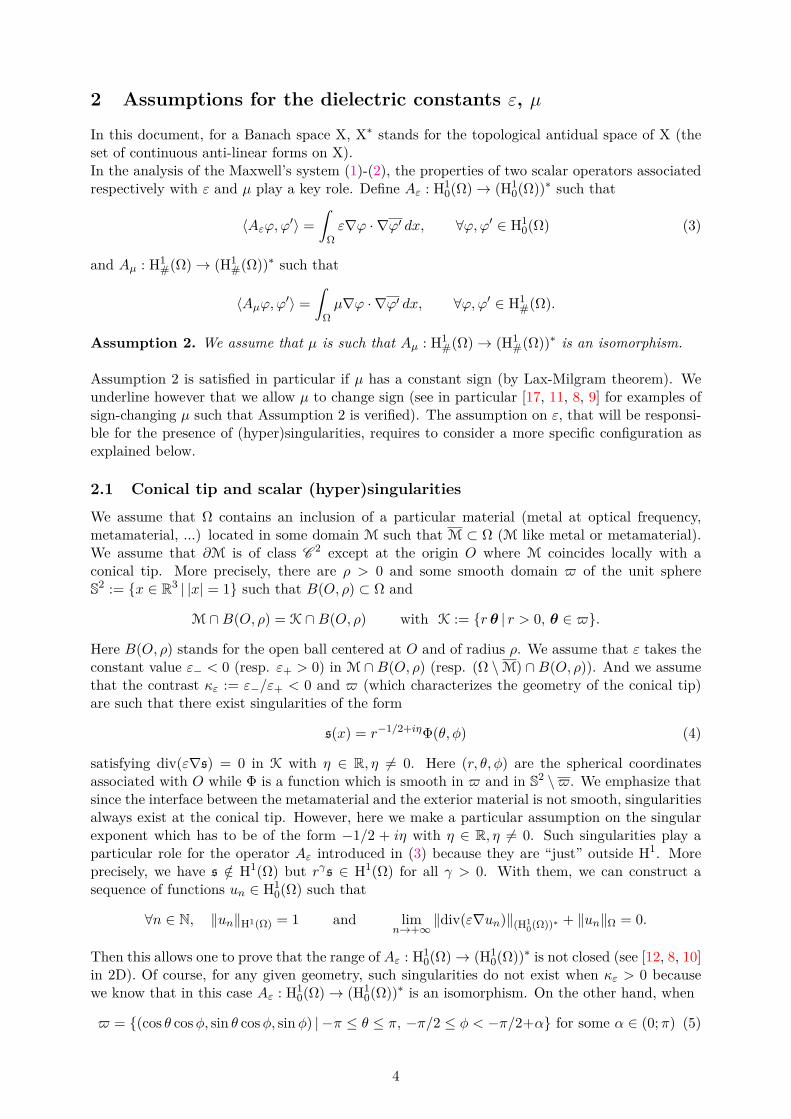
We assume that Ω contains an inclusion of a particular material (metal at optical frequency,metamaterial, ...) located in some domain M such that M ⊂ Ω (M like metal or metamaterial).We assume that ∂M is of class C 2 except at the origin O where M coincides locally with aconical tip. More precisely, there are ρ > 0 and some smooth domain $ of the unit sphereS2 := x ∈ R3 | |x| = 1 such that B(O, ρ) ⊂ Ω and

M ∩B(O, ρ) = K ∩B(O, ρ) with K := r θ | r > 0, θ ∈ $.

Here B(O, ρ) stands for the open ball centered at O and of radius ρ. We assume that ε takes theconstant value ε− < 0 (resp. ε+ > 0) in M ∩B(O, ρ) (resp. (Ω \M) ∩B(O, ρ)). And we assumethat the contrast κε := ε−/ε+ < 0 and $ (which characterizes the geometry of the conical tip)are such that there exist singularities of the form

s(x) = r−1/2+iηΦ(θ, φ) (4)

satisfying div(ε∇s) = 0 in K with η ∈ R, η 6= 0. Here (r, θ, φ) are the spherical coordinatesassociated with O while Φ is a function which is smooth in $ and in S2 \$. We emphasize thatsince the interface between the metamaterial and the exterior material is not smooth, singularitiesalways exist at the conical tip. However, here we make a particular assumption on the singularexponent which has to be of the form −1/2 + iη with η ∈ R, η 6= 0. Such singularities play aparticular role for the operator Aε introduced in (3) because they are “just” outside H1. Moreprecisely, we have s /∈ H1(Ω) but rγs ∈ H1(Ω) for all γ > 0. With them, we can construct asequence of functions un ∈ H1

0(Ω) such that

∀n ∈ N, ‖un‖H1(Ω) = 1 and limn→+∞

‖div(ε∇un)‖(H10(Ω))∗ + ‖un‖Ω = 0.

Then this allows one to prove that the range of Aε : H10(Ω)→ (H1

0(Ω))∗ is not closed (see [12, 8, 10]in 2D). Of course, for any given geometry, such singularities do not exist when κε > 0 becausewe know that in this case Aε : H1

0(Ω)→ (H10(Ω))∗ is an isomorphism. On the other hand, when

$ = (cos θ cosφ, sin θ cosφ, sinφ) | −π ≤ θ ≤ π, −π/2 ≤ φ < −π/2+α for some α ∈ (0;π) (5)

4

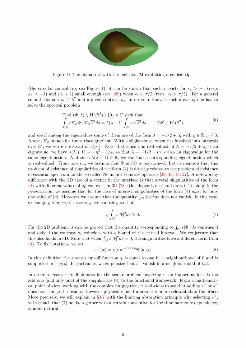
Figure 1: The domain Ω with the inclusion M exhibiting a conical tip.

(the circular conical tip, see Figure 1), it can be shown that such s exists for κε > −1 (resp.κε < −1) and |κε + 1| small enough (see [28]) when α < π/2 (resp. α > π/2). For a generalsmooth domain $ ⊂ S2 and a given contrast κε, in order to know if such s exists, one has tosolve the spectral problem

Find (Φ, λ) ∈ H1(S2) \ 0 × C such thatˆS2ε∇SΦ · ∇SΦ′ ds = λ(λ+ 1)

ˆS2εΦ Φ′ ds, ∀Φ′ ∈ H1(S2), (6)

and see if among the eigenvalues some of them are of the form λ = −1/2 + iη with η ∈ R, η 6= 0.Above, ∇S stands for the surface gradient. With a slight abuse, when ε is involved into integralsover S2, we write ε instead of ε(ρ ·). Note that since ε is real-valued, if λ = −1/2 + iη is aneigenvalue, we have λ(λ + 1) = −η2 − 1/4, so that λ = −1/2 − iη is also an eigenvalue for thesame eigenfunction. And since λ(λ + 1) ∈ R, we can find a corresponding eigenfunction whichis real-valued. From now on, we assume that Φ in (4) is real-valued. Let us mention that thisproblem of existence of singularities of the form (4) is directly related to the problem of existenceof essential spectrum for the so-called Neumann-Poincare operator [29, 43, 13, 27]. A noteworthydifference with the 2D case of a corner in the interface is that several singularities of the form(4) with different values of |η| can exist in 3D [28] (this depends on ε and on $). To simplify thepresentation, we assume that for the case of interest, singularities of the form (4) exist for onlyone value of |η|. Moreover we assume that the quantity

´S2 ε|Φ|2ds does not vanish. In this case,

exchanging η by −η if necessary, we can set η so that

η

ˆS2ε|Φ|2ds > 0. (7)

For the 2D problem, it can be proved that the quantity corresponding to´S2 ε|Φ|2ds vanishes if

and only if the contrast κε coincides with a bound of the critical interval. We conjecture thatthis also holds in 3D. Note that when

´S2 ε|Φ|2ds = 0, the singularities have a different form from

(4). To fix notations, we sets±(x) = χ(r)r−1/2±iηΦ(θ, φ) (8)

In this definition the smooth cut-off function χ is equal to one in a neighbourhood of 0 and issupported in [−ρ; ρ]. In particular, we emphasize that s± vanish in a neighbourhood of ∂Ω.

In order to recover Fredholmness for the scalar problem involving ε, an important idea is tooadd one (and only one) of the singularities (8) to the functional framework. From a mathemati-cal point of view, working with the complex conjugation, it is obvious to see that adding s+ or s−does not change the results. However physically one framework is more relevant than the other.More precisely, we will explain in §3.7 with the limiting absorption principle why selecting s+,with η such that (7) holds, together with a certain convention for the time-harmonic dependence,is more natural.

5

2.2 Kondratiev functional framework

In this paragraph, adapting what is done in [10] for the 2D case, we describe in more details howto get a Fredholm operator for the scalar operator associated with ε. For β ∈ R and m ∈ N, letus introduce the weighted Sobolev (Kondratiev) space Vm

β (Ω) (see [30]) defined as the closure ofC∞0 (Ω \ O) for the norm

‖ϕ‖Vmβ

(Ω) =

∑|α|≤m

‖r|α|−m+β∂αxϕ‖2L2(Ω)

1/2

.

Here C∞0 (Ω \ O) denotes the space of infinitely differentiable functions which are supported inΩ \ O. We also denote V1

β(Ω) the closure of C∞0 (Ω \ O) for the norm ‖ · ‖V1β

(Ω). We have thecharacterisation

V1β(Ω) = ϕ ∈ V1

β(Ω) |ϕ = 0 on ∂Ω.

Note that using Hardy’s inequalityˆ 1

0

|u(r)|2

r2 r2dr ≤ 4ˆ 1

0|u′(r)|2 r2dr, ∀u ∈ C 1

0 [0; 1),

one can show the estimate ‖r−1ϕ‖Ω ≤ C ‖∇ϕ‖Ω for all ϕ ∈ C∞0 (Ω \ O). This proves thatV1

0(Ω) = H10(Ω). Now set β > 0. Observe that we have

V1−β(Ω) ⊂ H1

0(Ω) ⊂ V1β(Ω) so that (V1

β(Ω))∗ ⊂ (H10(Ω))∗ ⊂ (V1

−β(Ω))∗.

Define the operators A±βε : V1±β(Ω)→ (V1

∓β(Ω))∗ such that

〈A±βε ϕ,ϕ′〉 =ˆ

Ωε∇ϕ · ∇ϕ′ dx, ∀ϕ ∈ V1

±β(Ω), ϕ′ ∈ V1∓β(Ω). (9)

Working as in [10] for the 2D case of the corner, one can show that there is β0 > 0 (depending onlyon κε and $) such that for all β ∈ (0;β0), Aβε is Fredholm of index +1 while A−βε is Fredholmof index −1. We remind the reader that for a bounded linear operator between two Banachspaces T : X→ Y whose range is closed, its index is defined as indT := dim ker T −dim coker T ,with dim coker T = dim (Y/range(T )). On the other hand, application of Kondratiev calculusguarantees that if ϕ ∈ V1

β(Ω) is such that A+βε ϕ ∈ (V1

β(Ω))∗ (the important point here being that(V1

β(Ω))∗ ⊂ (V1−β(Ω))∗), then there holds the following representation

ϕ = c− s− + c+ s

+ + ϕ with c± ∈ C and ϕ ∈ V1−β(Ω). (10)

Note that s±, with s± defined by (8), belongs to V1β(Ω), but not to H1

0(Ω), and a fortiori not toV1−β(Ω). Then introduce the space Vout := span(s+) ⊕ V1

−β(Ω), endowed with the norm

‖ϕ‖Vout = (|c|2 + ‖ϕ‖2V1−β(Ω)))

1/2, ∀ϕ = c s+ + ϕ ∈ Vout, (11)

which is a Banach space. Introduce also the operator Aoutε such that for all ϕ = c s+ + ϕ ∈ Vout

and ϕ′ ∈ C∞0 (Ω \ O),

〈Aoutε ϕ,ϕ′〉 =

ˆΩε∇ϕ · ∇ϕ′ dx = −c

ˆΩ

div(ε∇s+)ϕ′ dx+ˆ

Ωε∇ϕ · ∇ϕ′ dx.

Note that due to the features of the cut-off function χ, we have div(ε∇s+) ∈ L2(Ω). And sincediv(ε∇s+) = 0 in a neighbourhood of O, we observe that there is a constant C > 0 such that

6

|〈Aoutε ϕ,ϕ′〉| ≤ C ‖ϕ‖Vout ‖ϕ′‖V1

β(Ω). The density of C∞0 (Ω \ O) in V1

β(Ω) then allows us toextend Aout

ε as a continuous operator from Vout to (V1β(Ω))∗. And we have

〈Aoutε ϕ,ϕ′〉 = −c

ˆΩ

div(ε∇s+)ϕ′ dx+ˆ

Ωε∇ϕ · ∇ϕ′ dx, ∀ϕ = c s+ + ϕ, ϕ′ ∈ V1

β(Ω).

Working as in [10] (see Proposition 4.4.) for the 2D case of the corner, one can prove thatAoutε : Vout → (V1

β(Ω))∗ is Fredholm of index zero and that ker Aoutε = ker A−βε . In order to

simplify the analysis below, we shall make the following assumption.

Assumption 3. We assume that ε is such that for β ∈ (0;β0), A−βε is injective, which guaranteesthat Aout

ε : Vout → (V1β(Ω))∗ is an isomorphism.

In what follows, we shall also need to work with the usual Laplace operator in weighted Sobolevspaces. For γ ∈ R, define Aγ : V1

γ(Ω)→ (V1−γ(Ω))∗ such that

〈Aγϕ,ϕ′〉 =ˆ

Ω∇ϕ · ∇ϕ′ dx, ∀ϕ ∈ V1

γ(Ω), ϕ′ ∈ V1−γ(Ω)

(observe that there is no ε here). Combining the theory presented in [32] (see also the foundingarticle [30] as well as the monographs [34, 36]) together with the result of [31, Corollary 2.2.1],we get the following proposition.

Proposition 2.1. For all γ ∈ (−1/2; 1/2), the operator Aγ : V1γ(Ω)→ (V1

−γ(Ω))∗ is an isomor-phism.

Note in particular that for γ = 0, this proposition simply says that ∆ : H10(Ω)→ (H1

0(Ω))∗ is anisomorphism. In order to have a result of isomorphism both for Aout

ε and Aβ, we shall often makethe assumption that the weight β is such that

0 < β < min(1/2, β0) (12)

where β0 is defined after (9).To measure electromagnetic fields in weighted Sobolev norms, in the following we shall work inthe spaces

V0β(Ω) := (V0

β(Ω))3

V1β(Ω) := (V1

β(Ω))3.

Note that we have V0−β(Ω) ⊂ L2(Ω) ⊂ V0

β(Ω).

3 Analysis of the problem for the electric component

In this section, we consider the problem for the electric field associated with (1)-(2). Since thescalar problem involving ε is well-posed in a non standard framework involving the propagatingsingularity s+ (see (11)), we shall add its gradient in the space for the electric field. Then wedefine a variational problem in this unsual space, and prove its well-posedness. Finally we justifyour choice by a limiting absorption principle.

3.1 A well-chosen space for the electric field

Define the space of electric fields with the divergence free condition

XoutN (ε) := u = c∇s+ + u, c ∈ C, u ∈ L2(Ω) | curlu ∈ L2(Ω), div(εu) = 0 in Ω \ O,

u× ν = 0 on ∂Ω. (13)

7

In this definition, for u = c∇s+ + u, the condition div(εu) = 0 in Ω\O means that there holdsˆΩεu · ∇ϕdx = 0, ∀ϕ ∈ C∞0 (Ω \ O), (14)

which after integration by parts and by density of C∞0 (Ω \ O) in H10(Ω) is equivalent to

− cˆ

Ωdiv(ε∇s+)ϕdx+

ˆΩεu · ∇ϕdx = 0, ∀ϕ ∈ C∞0 (Ω). (15)

Note that we have XN (ε) ⊂ XoutN (ε) and that dim (Xout

N (ε)/XN (ε)) = 1 (see Lemma D.1 inAppendix). For u = c∇s+ + u with c ∈ C and u ∈ L2(Ω), we set

‖u‖XoutN (ε) = (|c|2 + ‖u‖2Ω + ‖curlu‖2Ω)1/2 .

Endowed with this norm, XoutN (ε) is a Banach space.

Lemma 3.1. Pick some β satisfying (12). Under Assumptions 1 and 3, for any u = c∇s+ + u ∈XoutN (ε), we have u ∈ V0

−β(Ω) and there is a constant C > 0 independent of u such that

|c|+ ‖u‖V0−β(Ω) ≤ C ‖curlu‖Ω. (16)

As a consequence, the norm ‖·‖XoutN (ε) is equivalent to the norm ‖curl ·‖Ω in Xout

N (ε) and XoutN (ε)

endowed with the inner product (curl ·, curl ·)Ω is a Hilbert space.Proof. Let u = c∇s+ + u be an element of Xout

N (ε). The field u is in L2(Ω) and thereforedecomposes as

u = ∇ϕ+ curlψ (17)with ϕ ∈ H1

0(Ω) and ψ ∈ XT (1) (item iv) of Proposition A.1). Moreover, since u× ν = 0 on ∂Ωand since both s+ and ϕ vanish on ∂Ω, we know that curlψ × ν = 0 on ∂Ω. Then noting that−∆ψ = curl u = curlu ∈ L2(Ω), we deduce from Proposition A.2 that curlψ ∈ V0

−β(Ω) withthe estimate

‖curlψ‖V0−β(Ω) ≤ C ‖curlu‖Ω. (18)

Using (14), the condition div(εu) = 0 in Ω \ O impliesˆΩε∇(c s+ + ϕ) · ∇ϕ′ dx = −

ˆΩεcurlψ · ∇ϕ′ dx, ∀ϕ′ ∈ V1

−β(Ω),

which means exactly that Aβε (c s+ + ϕ) = −div(ε curlψ) ∈ (V1−β(Ω))∗. Since additionally

−div(ε curlψ) ∈ (V1β(Ω))∗, from (10) we know that there are some complex constants c± and

some ϕ ∈ V1−β(Ω) such that

c s+ + ϕ = c− s− + c+ s

+ + ϕ.

This implies c− = 0, c+ = c (because ϕ ∈ H10(Ω)) and so ϕ = ϕ is an element of V1

−β(Ω). Thisshows that c s++ϕ ∈ Vout and thatAout

ε (c s++ϕ) = −div(ε curlψ). SinceAoutε : Vout → (V1

β(Ω))∗is an isomorphism, we have the estimate

|c|+ ‖ϕ‖V1−β(Ω) ≤ C ‖div(ε curlψ)‖(V1

β(Ω))∗ ≤ C ‖curlψ‖V0

−β(Ω). (19)

Finally gathering (17)–(19), we obtain that u ∈ V0−β(Ω) and that the estimate (16) is valid.

Noting that ‖u‖Ω ≤ C ‖u‖V0−β(Ω), this implies that the norms ‖ · ‖Xout

N (ε) and ‖curl · ‖Ω areequivalent in Xout

N (ε).

Thanks to the previous lemma and by density of C∞0 (Ω \ O) in V1β(Ω), the condition (15) for

u = c∇s+ + u ∈ XoutN (ε) is equivalent to

− cˆ

Ωdiv(ε∇s+)ϕdx+

ˆΩεu · ∇ϕdx = 0, ∀ϕ ∈ V1

β(Ω) (20)

where all the terms are well-defined as soon as β satisfies (12).

8

3.2 Definition of the problem for the electric field

Our objective is to define the problem for the electric field as a variational formulation set inXoutN (ε). For some γ > 0, let J be an element of V0

−γ(Ω) such that divJ = 0 in Ω. Consider theproblem

Find u ∈ XoutN (ε) such thatˆ

Ωµ−1curlu · curlv dx− ω2

Ωεu · v dx = iω

ˆΩJ · v dx, ∀v ∈ Xout

N (ε), (21)

where the term Ωεu · v dx (22)

has to be carefully defined. The difficulty comes from the fact that XoutN (ε) is not a subspace of

L2(Ω) so that this quantity cannot be considered as a classical integral.Let u = cu∇s+ + u ∈ Xout

N (ε). First, for v ∈ V0−β(Ω) with β > 0, it is natural to set

Ωεu · v dx :=

ˆΩεu · v dx. (23)

To complete the definition, we have to give a sense to (22) when v = ∇s+. Proceeding as for thederivation of (20), we start from the identity

ˆΩεu · ∇ϕdx = −cu

ˆΩ

div(ε∇s+)ϕdx+ˆ

Ωεu · ∇ϕdx, ∀ϕ ∈ C∞0 (Ω \ O).

By density of C∞0 (Ω \ O) in V1β(Ω), this leads to set

Ωεu · ∇ϕdx := −cu

ˆΩ

div(ε∇s+)ϕdx+ˆ

Ωεu · ∇ϕdx, ∀ϕ ∈ V1

β(Ω). (24)

With this definition, condition (20) can be written as

Ωεu · ∇ϕdx = 0, ∀ϕ ∈ V1

β(Ω).

In particular, since s+ ∈ V1β(Ω), for all u ∈ Xout

N (ε) we have

Ωεu · ∇s+ dx = 0 and so

ˆΩεu · ∇s+ dx = cu

ˆΩ

div(ε∇s+)s+ dx. (25)

Finally for all u = cu∇s+ + u and v = cv∇s+ + v in XoutN (ε), using (23) and (25), we find

Ωεu · v dx =

ˆΩεu · v dx = cu

ˆΩε∇s+ · v dx+

ˆΩεu · v dx.

But since v ∈ XoutN (ε), we deduce from the second identity of (25) that

ˆΩε∇s+ · v dx = cv

ˆΩ

div(ε∇s+)s+ dx. (26)

Summing up, we get

Ωεu · v dx = cucv

ˆΩ

div(ε∇s+)s+ dx+ˆ

Ωεu · v dx, ∀u,v ∈ Xout

N (ε). (27)

9

Remark 3.2. Even if we use an integral symbol to keep the usual aspects of formulas and facilitatethe reading, it is important to consider this new quantity as a sesquilinear form

(u,v) 7→

Ωεu · v dx

on XoutN (ε)×Xout

N (ε). In particular, we point out that this sesquilinear form is not hermitian onXoutN (ε)×Xout

N (ε). Indeed, we have

Ωεv · u dx =

ˆΩεu · v dx+ cucv

ˆΩ

div(ε∇s+)s+ dx

so that Ωεu · v dx−

Ωεv · u dx = 2icucv =m

(ˆΩ

div(ε∇s+) s+ dx

). (28)

But Lemma C.1 and assumption (7) show that

=m( ˆ

Ωdiv(ε∇s+) s+ dx

)6= 0.

In the sequel, we denote by aN (·, ·) (resp. `N (·)) the sesquilinear form (resp. the antilinear form)appearing in the left-hand side (resp. right-hand side) of (21).

3.3 Equivalent formulation

Define the spaceHoutN (curl ) := span(∇s+)⊕HN (curl ) ⊃ Xout

N (ε)

(without the divergence free condition) and consider the problem

Find u ∈ HoutN (curl ) such that

aN (u,v) = `N (v), ∀v ∈ HoutN (curl ),

(29)

where the definition of Ωεu · v dx

has to be extended to the space HoutN (curl ). Working exactly as in the beginning of the proof of

Lemma 3.1, one can show that any u ∈ HoutN (curl ) admits the decomposition

u = cu∇s+ +∇ϕu + curlψu, (30)

with cu ∈ C, ϕu ∈ H10(Ω) and ψu ∈ XT (1), such that curlψu ∈ V0

−β(Ω), for β satisfying (12).Then, for all u = cu∇s+ + ∇ϕu + curlψu and v = cv∇s+ + ∇ϕv + curlψv in Hout

N (curl ), anatural extension of the previous definitions leads to set

Ωεu · v dx :=

ˆΩε (∇ϕu + curlψu) · (∇ϕv + curlψv) dx

+ˆ

Ωcu ε∇s+ · curlψv + cv ε curlψu · ∇s+ dx

−ˆ

Ωcucv div(ε∇s+)s+ + cu div(ε∇s+)ϕv + cv ϕudiv(ε∇s+) dx.

(31)

Note that (31) is indeed an extension of (27). To show it, first observe that for u = cu∇s+ +∇ϕu+ curlψu, v = cv∇s+ +∇ϕv + curlψv in Xout

N (ε), the proof of Lemma 3.1 guarantees that

10

ϕu, ϕv ∈ V1−β(Ω) with β satisfying (12). This allows us to integrate by parts in the last two

terms of (31) to get

Ωεu · v dx :=

ˆΩε (∇ϕu + curlψu) · (∇ϕv + curlψv) dx

+ˆ

Ωcu ε∇s+ · (∇ϕv + curlψv) + cv ε (∇ϕu + curlψu) · ∇s+ dx

−cucvˆ

Ωdiv(ε∇s+)s+ dx.

(32)

Using (25), (26), the second line above can be written asˆ

Ωcu ε∇s+ · (∇ϕv + curlψv) + cv ε (∇ϕu + curlψu) · ∇s+ dx

= cucv

ˆΩ

div(ε∇s+)s+ dx+ cucv

ˆΩ

div(ε∇s+)s+ dx.

(33)

Inserting (33) in (32) yields exactly (27).

Lemma 3.3. Under Assumptions 1 and 3, the field u is a solution of (21) if and only if it solvesthe problem (29).

Proof. If u ∈ HoutN (curl ) satisfies (29), then taking v = ∇ϕ with ϕ ∈ C∞0 (Ω \ O) in (29), and

using that divJ = 0 in Ω, we get (14), which implies that u ∈ XoutN (ε). This shows that u solves

(21).

Now assume that u ∈ XoutN (ε) ⊂ Hout

N (curl ) is a solution of (21). Let v be an element ofHoutN (curl ). As in (30), we have the decomposition

v = cv∇s+ +∇ϕv + curlψv, (34)

with cv ∈ C, ϕv ∈ H10(Ω) and ψv ∈ XT (1) such that curlψv ∈ V0

−β(Ω) for all β satisfying (12).By Assumption 3, there is ζ ∈ Vout such that

Aoutε ζ = −div(ε curlψv) ∈ (V1

β(Ω))∗. (35)

The function ζ decomposes as ζ = αs+ + ζ with ζ ∈ V1−β(Ω). Finally, set

v = curlψv −∇ζ = v −∇(cvs+ + ϕv + ζ).

The function v is in XoutN (ε), it satisfies curl v = curlv and from (25), we deduce that

Ωεu · v dx =

Ωεu · v dx.

Using also that J ∈ V0−γ(Ω) for some γ > 0 and is such that divJ = 0 in Ω, so that

ˆΩJ · v dx =

ˆΩJ · v dx,

this shows that aN (u,v) = aN (u, v) = `N (v) = `N (v) and ends the proof.

In the following, we shall work with the formulation (21) set in XoutN (ε). The reason being that, as

usual in the analysis of Maxwell’s equations, the divergence free condition will yield a compactnessproperty allowing us to deal with the term involving the frequency ω.

11

3.4 Main analysis for the electric field

Define the continuous operators AoutN : Xout

N (ε) → (XoutN (ε))∗ and Kout

N : XoutN (ε) → (Xout

N (ε))∗such that for all u, v ∈ Xout

N (ε),

〈AoutN u,v〉 =

ˆΩµ−1curlu · curlv dx, 〈Kout

N u,v〉 =

Ωεu · v dx.

With this notation, we have 〈(AoutN + Kout

N )u,v〉 = aN (u,v).

Proposition 3.4. Under Assumptions 1–3, the operator AoutN : Xout

N (ε) → (XoutN (ε))∗ is an

isomorphism.

Proof. Let us construct a continuous operator T : XoutN (ε) → Xout

N (ε) such that for all u, v ∈XoutN (ε), ˆ

Ωµ−1curlu · curl (Tv) dx =

ˆΩ

curlu · curlv dx.

To proceed, we adapt the method presented in [9]. Assume that v ∈ XoutN (ε) is given. We con-

struct Tv in three steps.

1) Since curlv ∈ L2(Ω) and Aµ : H1#(Ω) → (H1

#(Ω))∗ is an isomorphism, there is a uniqueζ ∈ H1

#(Ω) such thatˆ

Ωµ∇ζ · ∇ζ ′ dx =

ˆΩµ curlv · ∇ζ ′ dx, ∀ζ ′ ∈ H1

#(Ω).

Then the field µ(curlv−∇ζ) ∈ L2(Ω) is divergence free in Ω and satisfies µ(curlv−∇ζ) · ν = 0on ∂Ω.

2) From item ii) of Proposition A.1, we infer that there is ψ ∈ XN (1) such that

µ(curlv −∇ζ) = curlψ.

Thanks to Lemma A.5, we deduce that ψ ∈ V0−β(Ω) for all β ∈ (0; 1/2) and a fortiori for β

satisfying (12).

3) Suppose now that β satisfies (12). Then we know from the previous step that div(εψ) ∈(V1

β(Ω))∗. On the other hand, by Assumption 3, Aoutε : Vout → (V1

β(Ω))∗ is an isomorphism.Consequently we can introduce ϕ ∈ Vout such that Aout

ε ϕ = −div(εψ).

Finally, we set Tv = ψ − ∇ϕ. Clearly Tv is an element of XoutN (ε). Moreover, for all u, v

in XoutN (ε), we have

ˆΩµ−1curlu · curlTv dx =

ˆΩµ−1curlu · curlψ dx

=ˆ

Ωcurlu · curlv dx−

ˆΩ

curlu · ∇ζ dx

=ˆ

Ωcurlu · curlv dx.

From Lemma 3.1 and the Lax-Milgram theorem, we deduce that T∗AoutN : Xout

N (ε)→ (XoutN (ε))∗ is

an isomorphism. And by symmetry, permuting the roles of u and v, it is obvious that T∗AoutN =

AoutN T, which allows us to conclude that Aout

N : XoutN (ε)→ (Xout

N (ε))∗ is an isomorphism.

12

Proposition 3.5. Under Assumptions 1 and 3, if (un = cn∇s+ + un) is a sequence which isbounded in Xout

N (ε), then we can extract a subsequence such that (cn) and (un) converge respec-tively in C and in V0

−β(Ω) for β satisfying (12). As a consequence, the operator KoutN : Xout

N (ε)→(Xout

N (ε))∗ is compact.

Proof. Let (un) be a bounded sequence of elements of XoutN (ε). From the proof of Lemma 3.1,

we know that for n ∈ N, we have

un = cn∇s+ +∇ϕn + curlψn (36)

where the sequences (cn), (ϕn), (ψn) and (curlψn) are bounded respectively in C, V1−β(Ω),

XT (1) and V0−β(Ω). Observing that curlun = curl curlψn = −∆ψn is bounded in L2(Ω),

we deduce from Proposition A.3 that there exists a subsequence such that curlψn converges inV0−β(Ω). Moreover, by (19), we have

|cn − cm|+ ‖ϕn − ϕm‖V1−β(Ω) ≤ C‖curl (ψn −ψm)‖V0

−β(Ω),

which implies that (cn) and (ϕn) converge respectively in C and in V1−β(Ω). From (36), we see

that this is enough to conclude to the first part of the proposition.Finally, observing that

‖KoutN u‖(Xout

N (ε))∗ ≤ C (‖u‖V0−β(Ω) + |cu|),

we deduce that KoutN : Xout

N (ε)→ (XoutN (ε))∗ is a compact operator.

We can now state the main theorem of the analysis of the problem for the electric field.

Theorem 3.6. Under Assumptions 1–3, for all ω ∈ R the operator AoutN − ω2Kout

N : XoutN (ε) →

(XoutN (ε))∗ is Fredholm of index zero.

Proof. Since KoutN : Xout

N (ε) → (XoutN (ε))∗ is compact (Proposition 3.5) and Aout

N : XoutN (ε) →

(XoutN (ε))∗ is an isomorphism (Proposition 3.4), Aout

N −ω2KoutN : Xout

N (ε)→ (XoutN (ε))∗ is Fredholm

of index zero.

The previous theorem guarantees that the problem (21) is well-posed if and only if uniquenessholds, that is if and only if the only solution for J = 0 is u = 0. Since uniqueness holds for ω = 0,one can prove with the analytic Fredholm theorem that (21) is well-posed except for at most acountable set of values of ω with no accumulation points (note that Theorem 3.6 remains truefor ω ∈ C).However this result is not really relevant from a physical point of view. Indeed, negative valuesof ε can occur only if ε is itself a function of ω. For instance, if the inclusion M is metallic, it iscommonly admitted that the Drude’s law gives a good model for ε. But taking into account thedependence of ε with respect to ω when studying uniqueness of problem (21) leads to a non-lineareigenvalue problem, where the functional space Xout

N (ε) itself depends on ω. This study is beyondthe scope of the present paper (see [24] for such questions in the case of the 2D scalar problem).Nonetheless, there is a result that we can prove concerning the cases of non-uniqueness for problem(21).

Proposition 3.7. If u = c∇s+ + u ∈ XoutN (ε) is a solution of (21) for J = 0, then c = 0 and

u ∈ XN (ε).

Proof. When ω = 0, the result is a direct consequence of Theorem 3.6 (because zero is theonly solution of (21) for J = 0). From now on, we assume that ω ∈ R \ 0. Suppose thatu = c∇s+ + u ∈ Xout

N (ε) is such thatˆ

Ωµ−1curlu · curlv dx− ω2

Ωεu · v dx = 0, ∀v ∈ Xout

N (ε).

13

Taking the imaginary part of the previous identity for v = u, we get

=m(

Ωεu · u dx

)= 0.

On the other hand, by (27), we have

Ωεu · u dx =

ˆΩε|u|2 dx+ |c|2

ˆΩ

div(ε∇s+) s+ dx,

so that|c|2=m

( ˆΩ

div(ε∇s+) s+ dx

)= 0.

The result of the proposition is then a consequence of Lemma C.1 in Appendix where it is provedthat

=m( ˆ

Ωdiv(ε∇s+) s+ dx

)= η

ˆS2ε|Φ|2ds,

and of the assumption (7).

Remark 3.8. As a consequence, from Lemma 3.1, we infer that elements of the kernel of AoutN −

ω2KoutN are in V0

−β(Ω) for all β satisfying (12).

3.5 Problem in the classical framework

In the previous paragraph, we have shown that the Maxwell’s problem (21) for the electric fieldset in the non standard space Xout

N (ε), and so in HoutN (curl ) according to Lemma 3.3, is well-

posed. Here, we wish to analyse the properties of the problem for the electric field set in theclassical space XN (ε) (which does not contain ∇s+). Since this space is a closed subspace ofXoutN (ε), it inherits the main properties of the problem in Xout

N (ε) proved in the previous section.More precisely, we deduce from Lemma 3.1 and Proposition 3.5 the following result.

Proposition 3.9. Under Assumptions 1 and 3, the embedding of XN (ε) in L2(Ω) is compact,and ‖curl · ‖Ω is a norm in XN (ε) which is equivalent to the norm ‖ · ‖H(curl ).

Note that we recover classical properties similar to what is known for positive ε, or more generally[9] for ε such that the operator Aε : H1

0(Ω)→ (H10(Ω))∗ defined by (3) is an isomorphism (which

allows for sign-changing ε). But we want to underline the fact that under Assumption 3, theseclassical results could not be proved by using classical arguments. They require the introductionof the bigger space Xout

N (ε), with the singular function ∇s+.Let us now consider the problem

Find u ∈ XN (ε) such thatˆΩµ−1curlu · curlv dx− ω2

ˆΩεu · v dx = iω

ˆΩJ · v dx, ∀v ∈ XN (ε). (37)

An important remark is that one cannot prove that problem (37) is equivalent to a similar problemset in HN (curl ) (the analogue of Lemma 3.3). Again, the difficulty comes from the fact that Aεis not an isomorphism, and the trouble would appear when solving (35). Therefore, a solution of(37) is not in general a distributional solution of the equation

curl(µ−1curlu

)− ω2εu = iωJ .

To go further in the analysis of (37), we recall that XN (ε) is a subspace of codimension one ofXoutN (ε) (Lemma D.1 in Appendix). Let v0 be an element of Xout

N (ε) which does not belong toXN (ε). Then we denote by `0 the continuous linear form on Xout

N (ε) such that:

∀v ∈ XoutN (ε) v − `0(v)v0 ∈ XN (ε). (38)

14

Let us now define the operators AN : XN (ε)→ (XN (ε))∗ and KN : XN (ε)→ (XN (ε))∗ by

〈ANu,v〉 =ˆ

Ωµ−1curlu · curlv dx, 〈KNu,v〉 =

ˆΩεu · v dx.

Proposition 3.10. Under Assumptions 1–3, the operator AN : XN (ε)→ (XN (ε))∗ is Fredholmof index zero.

Proof. Let u ∈ XN (ε). By Proposition 3.4, for the operator T introduced in the correspondingproof, one has:

‖u‖2XN (ε) = ‖curlu‖2Ω = 〈AoutN u,Tu〉.

Then, using (38), we get:

‖u‖2XN (ε) = 〈ANu,Tu− `0(Tu)v0〉+ 〈AoutN u, `0(Tu)v0〉,

which implies that‖u‖XN (ε) ≤ C

(‖ANu‖(XN (ε))∗ + |`0(Tu)|

).

The result of the proposition then follows from a classical adaptation of Peetre’s lemma (see forexample [48, Theorem 12.12]) together with the fact that AN is bounded and hermitian.

Combining the two previous propositions, we obtain the

Theorem 3.11. Under Assumptions 1–3, for all ω ∈ R, the operator AN − ω2KN : XN (ε) →(XN (ε))∗ is Fredholm of index zero.

But as mentioned above, even if uniqueness holds and if Problem (37) is well-posed, it does notprovide a solution of Maxwell’s equations.

3.6 Expression of the singular coefficient

Under Assumptions 1–3, Theorem 3.6 guarantees that for all ω ∈ R the operator AoutN − ω2Kout

N :XoutN (ε)→ (Xout

N (ε))∗ is Fredholm of index zero. Assuming that it is injective, the problem (21)admits a unique solution u = cu∇s+ + u. The goal of this paragraph is to derive a formulaallowing one to compute cu without knowing u. Such kind of results are classical for scalar op-erators (see e.g. [22], [32, Theorem 6.4.4], [18, 19, 2, 23, 49, 40]). They are used in particular fornumerical purposes. But curiously they do not seem to exist for Maxwell’s equations in 3D, noteven for classical situations with positive materials in non smooth domains. We emphasize thatthe analysis we develop can be adapted to the latter case.

In order to establish the desired expression, for ω ∈ R, first we introduce the field wN ∈ XoutN (ε)

such thatˆΩµ−1curlv · curlwN dx− ω2

Ωεv ·wN dx =

ˆΩεv · ∇s+ dx, ∀v ∈ Xout

N (ε). (39)

Note that Problem (39) is well-posed when AoutN −ω2Kout

N is an isomorphism. Indeed, using (28),one can check that it involves the operator (Aout

N −ω2KoutN )∗, that is the adjoint of Aout

N −ω2KoutN .

Moreover v 7→´

Ω εv · ∇s+ dx is a linear form over XoutN (ε).

Theorem 3.12. Assume that ω ∈ R, Assumptions 1–3 are valid and AoutN − ω2Kout

N : XoutN (ε)→

(XoutN (ε))∗ is injective. Then the solution u = cu∇s+ + u of the electric problem (21) is such that

cu = iω

ˆΩJ ·wN dx

/ ˆΩ

div(ε∇s+) s+ dx. (40)

Here wN is the function which solves (39).

15

Remark 3.13. Note that in practice wN can be computed once for all because it does not dependon J . Then the value of cu can be determined very simply via Formula (40).

Proof. By definition of u, we haveˆ

Ωµ−1curlu · curlwN dx− ω2

Ωεu ·wN dx = iω

ˆΩJ ·wN dx.

On the other hand, from (39), there holdsˆ

Ωµ−1curlu · curlwN dx− ω2

Ωεu ·wN dx =

ˆΩεu · ∇s+ dx.

From these two relations as well as (25), we get

iω

ˆΩJ ·wN dx =

ˆΩεu · ∇s+ dx = cu

ˆΩ

div(ε∇s+) s+ dx.

But Lemma C.1 in Appendix guarantees that =m´

Ω div(ε∇s+) s+ dx 6= 0. Therefore we find thedesired formula.

3.7 Limiting absorption principle

In §3.4, we have proved well-posedness of the problem for the electric field in the space XoutN (ε).

But up to now, we have not explained why we select this framework. In particular, as mentionedin §2.1, well-posedness also holds in Xin

N (ε) where XinN (ε) is defined as Xout

N (ε) with s+ replacedby s− (see (8) for the definitions of s±). In general, the solution in Xin

N (ε) differs from the onein Xout

N (ε). Therefore one can build infinitely many solutions of Maxwell’s problem as linearinterpolations of these two solutions. Then the question is: which solution is physically relevant?Classically, the answer can be obtained thanks to the limiting absorption principle. The idea isthe following. In practice, the dielectric permittivity takes complex values, the imaginary partbeing related to the dissipative phenomena in the materials. Set

εδ := ε+ iδ

where ε is defined as previously (see (2)) and δ > 0 (the sign of δ depends on the convention for thetime-harmonic dependence (in e−iωt here)). Due to the imaginary part of εδ which is uniformlypositive, one recovers some coercivity properties which allow one to prove well-posedness of thecorresponding problem for the electric field in the classical framework. The physically relevantsolution for the problem with the real-valued ε then should be the limit of the sequence of solutionsfor the problems involving εδ when δ tends to zero. The goal of the present paragraph is to explainhow to show that this limit is the solution of the problem set in Xout

N (ε).

3.7.1 Limiting absorption principle for the scalar case

Our proof relies on a similar result for the 3D scalar problem which is the analogue of what hasbeen done in 2D in [9, Theorem 4.3]. Consider the problem

Find ϕδ ∈ H10(Ω) such that − div(εδ∇ϕδ) = f, (41)

where f ∈ (H10(Ω))∗. Since δ > 0, by the Lax-Milgram lemma, this problem is well-posed for all

f ∈ (H10(Ω))∗ and in particular for all f ∈ (V1

β(Ω))∗, β > 0. Our objective is to prove that ϕδconverges when δ tends to zero to the unique solution of the problem

Find ϕ ∈ Vout such that Aoutε ϕ = f. (42)

16

We expect a convergence in a space V1β(Ω) with 0 < β < β0. We first need a decomposition of

ϕδ as a sum of a singular part and a regular part. Since problem (41) is strongly elliptic, one candirectly apply the theory presented in [32]. On the one hand, from the assumptions of Section 2,one can verify that for δ small enough, there exists one and only one singular exponent λδ ∈ Csuch that <e λδ ∈ (−1/2;−1/2 + β0 −

√δ). We denote by sδ the corresponding singular function

such thatsδ(r, θ, ϕ) = rλ

δ Φδ(θ, φ).Note that it satisfies div(εδ∇sδ) = 0 in K. As in (8) for s±, we set

sδ(x) = χ(r) r−1/2+iηδ Φδ(θ, φ), (43)where ηδ ∈ C is the number such that λδ = −1/2 + iηδ. By applying [32, Theorem 5.4.1], we getthe following result.Lemma 3.14. Let 0 < β < β0 and f ∈ (V1

β(Ω))∗. The solution ϕδ of (41) decomposes as

ϕδ = cδsδ + ϕδ (44)where cδ ∈ C and ϕδ ∈ V1

−β(Ω).Let us first study the limit of the singular function.Lemma 3.15. For all β > 0, when δ tends to zero, the function sδ converges in V1

β(Ω) to s+

and not to s− (see the definitions in (8)).Proof. The pair (Φδ, λδ) solves the spectral problem

Find (Φδ, λδ) ∈ H1(S2) \ 0 × C such thatˆS2εδ∇SΦδ · ∇SΨ ds = λδ(λδ + 1)

ˆS2εδΦδ Ψ ds, ∀Ψ ∈ H1(S2). (45)

Postulating the expansions Φδ = Φ0+δΦ′+. . . , λδ = λ0+δλ′+. . . in this problem and identifyingthe terms in δ0, we get Φ0 = Φ and we find that λ0 = −1/2 + iη0 where η0 coincides with η or−η (see an illustration with Figure 2). At order δ, we get the variational equalityˆ

S2ε∇SΦ′ · ∇SΨ ds+ i

ˆS2∇SΦ · ∇SΨ ds = λ0(λ0 + 1)

( ˆS2εΦ′Ψ ds+ i

ˆS2

Φ Ψ ds

)+λ′(2λ0 + 1)

ˆS2εΦ Ψ ds, ∀Ψ ∈ H1(S2).

(46)

Taking Ψ = Φ in (46), using (6) and observing that λ0(λ0 + 1) = −η2 − 1/4, this impliesˆS2|∇SΦ|2 + (η2 + 1/4)|Φ|2 ds = λ′2η0

ˆS2ε|Φ|2 ds.

Thus λ′ is real. Since by definition of λδ, we have <e λδ > −1/2 for δ > 0, we infer that λ′ > 0.As a consequence, we have

η0ˆS2ε|Φ|2 ds > 0

which according to the definition of η in (7) ensures that η0 = η. Therefore the pointwise limitof sδ when δ tends to zero is indeed s+ and not s−. This is enough to conclude that sδ convergesto s+ in V1

β(Ω) for β > 0.

Then proceeding exactly as in the proof of [10, Theorem 4.3], one can establish the followingresult.Lemma 3.16. Let 0 < β < β0 and f ∈ (V1

β(Ω))∗. If Assumption 3 holds, then (ϕδ = cδ sδ + ϕδ)converges to ϕ = c s+ + ϕ in V1

β(Ω) as δ tends to zero. Moreover, (cδ, ϕδ) converges to (c, ϕ) inC× V1

−β(Ω). In this statement, ϕδ (resp. ϕ) is the solution of (41) (resp. (42)).Note that the results of Lemma 3.16 still hold if we replace f by a family of source terms(f δ) ∈ (V1

β(Ω))∗ that converges to f in (V1β(Ω))∗ when δ tends to zero.

17

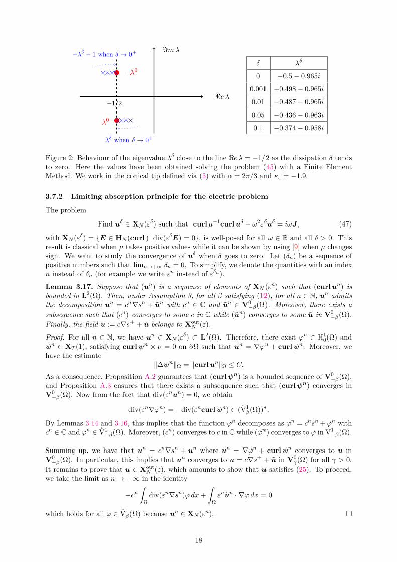
−λ0

λ0

<e λ

=mλ

−1/2

−λδ − 1 when δ → 0+

λδ when δ → 0+

δ λδ

0 −0.5− 0.965i

0.001 −0.498− 0.965i

0.01 −0.487− 0.965i

0.05 −0.436− 0.963i

0.1 −0.374− 0.958i

Figure 2: Behaviour of the eigenvalue λδ close to the line <e λ = −1/2 as the dissipation δ tendsto zero. Here the values have been obtained solving the problem (45) with a Finite ElementMethod. We work in the conical tip defined via (5) with α = 2π/3 and κε = −1.9.

3.7.2 Limiting absorption principle for the electric problem

The problem

Find uδ ∈ XN (εδ) such that curlµ−1curluδ − ω2εδuδ = iωJ , (47)

with XN (εδ) = E ∈ HN (curl ) | div(εδE) = 0, is well-posed for all ω ∈ R and all δ > 0. Thisresult is classical when µ takes positive values while it can be shown by using [9] when µ changessign. We want to study the convergence of uδ when δ goes to zero. Let (δn) be a sequence ofpositive numbers such that limn→+∞ δn = 0. To simplify, we denote the quantities with an indexn instead of δn (for example we write εn instead of εδn).

Lemma 3.17. Suppose that (un) is a sequence of elements of XN (εn) such that (curlun) isbounded in L2(Ω). Then, under Assumption 3, for all β satisfying (12), for all n ∈ N, un admitsthe decomposition un = cn∇sn + un with cn ∈ C and un ∈ V0

−β(Ω). Moreover, there exists asubsequence such that (cn) converges to some c in C while (un) converges to some u in V0

−β(Ω).Finally, the field u := c∇s+ + u belongs to Xout

N (ε).

Proof. For all n ∈ N, we have un ∈ XN (εδ) ⊂ L2(Ω). Therefore, there exist ϕn ∈ H10(Ω) and

ψn ∈ XT (1), satisfying curlψn × ν = 0 on ∂Ω such that un = ∇ϕn + curlψn. Moreover, wehave the estimate

‖∆ψn‖Ω = ‖curlun‖Ω ≤ C.As a consequence, Proposition A.2 guarantees that (curlψn) is a bounded sequence of V0

−β(Ω),and Proposition A.3 ensures that there exists a subsequence such that (curlψn) converges inV0−β(Ω). Now from the fact that div(εnun) = 0, we obtain

div(εn∇ϕn) = −div(εncurlψn) ∈ (V1β(Ω))∗.

By Lemmas 3.14 and 3.16, this implies that the function ϕn decomposes as ϕn = cnsn + ϕn withcn ∈ C and ϕn ∈ V1

−β(Ω). Moreover, (cn) converges to c in C while (ϕn) converges to ϕ in V1−β(Ω).

Summing up, we have that un = cn∇sn + un where un = ∇ϕn + curlψn converges to u inV0−β(Ω). In particular, this implies that un converges to u = c∇s+ + u in V0

γ(Ω) for all γ > 0.It remains to prove that u ∈ Xout

N (ε), which amounts to show that u satisfies (25). To proceed,we take the limit as n→ +∞ in the identity

−cnˆ

Ωdiv(εn∇sn)ϕdx+

ˆΩεnun · ∇ϕdx = 0

which holds for all ϕ ∈ V1β(Ω) because un ∈ XN (εn).

18

Theorem 3.18. Let ω ∈ R. Suppose that Assumptions 1, 2 and 3 hold, and that u = 0 is theonly function of XN (ε) satisfying

curlµ−1curlu− ω2εu = 0. (48)

Then the sequence of solutions (uδ = cδ∇sδ+uδ) of (47) converges, as δ tends to 0, to the uniquesolution u = c∇s+ + u ∈ Xout

N (ε) of (21) in the following sense: (cδ) converges to c in C, (uδ)converges to u in V0

−β(Ω) and (curluδ) converges to curlu in L2(Ω).

Proof. Let (δn) be a sequence of positive numbers such that limn→+∞ δn = 0. Denote by un theunique function of XN (εn) such that

curlµ−1curlun − ω2εnun = iωJ . (49)

Note that we set again εn instead of εδn . The proof is in two steps. First, we establish the desiredproperty by assuming that (‖curlun‖Ω) is bounded. Then we show that this hypothesis is indeedsatisfied.First step. Assume that there is a constant C > 0 such that for all n ∈ N

‖curlun‖Ω ≤ C. (50)

By lemma 3.17, we can extract a subsequence from (un = cn∇sn + un) such that (cn) convergesto c in C, (un) converges to u in V0

−β(Ω), with u = u + c∇s+ ∈ XoutN (ε). Besides, since for all

n ∈ N, curlun ∈ L2(Ω), there exist hn ∈ H1#(Ω) and wn ∈ XN (1), such that

µ−1curlun = ∇hn + curlwn. (51)

Observing that (wn) is bounded in XN (1), from Lemma A.5, we deduce that it admits asubsequence which converges in V0

−β(Ω). Multiplying (49) taken for two indices n and m by(wn −wm), and integrating by parts, we obtain

ˆΩ|curlwn − curlwm|2 dx = ω2

ˆΩ

(εnun − εmum) (wn −wm) dx.

This implies that (curlwn) converges in L2(Ω). Then, from (51), we deduce that

div (µ∇hn) = −div (µ curlwn) in Ω.

By Assumption 2, the operator Aµ : H1#(Ω) → (H1

#(Ω))∗ is an isomorphism. Therefore (∇hn)converges in L2(Ω). From (51), this shows that (curlun) converges to curlu in L2(Ω). Finally,we know that un satisfiesˆ

Ωµ−1curlun · curlv dx− ω2

ˆΩεnun · v dx = iω

ˆΩJ · v dx

for all v ∈ V0−β(Ω). Taking the limit, we get that u satisfies

ˆΩµ−1curlu · curlv dx− ω2

Ωεu · v dx = iω

ˆΩJ · v dx (52)

for all v ∈ V0−β(Ω). Since in addition, u satisfies (25), (52) also holds for v = ∇s+ and we get

that u is the unique solution u of (21).Second step. Now we prove that the assumption (50) is satisfied. Suppose by contradictionthat there exists a subsequence of (un) such that

‖curlun‖Ω → +∞

19

and consider the sequence (vn) with for all n ∈ N, vn := un/‖curlun‖Ω. We have

vn ∈ XN (εn) and curlµ−1curlvn − ω2εnvn = iωJ/‖curlun‖Ω. (53)

Following the first step of the proof, we find that we can extract a subsequence from (vn) whichconverges, in the sense given in the theorem, to the unique solution of the homogeneous problem(21) with J = 0. But by Proposition 3.7, this solution also solves (48). As a consequence, itis equal to zero. In particular, it implies that (curlvn) converges to zero in L2(Ω), which isimpossible since by construction, for all n ∈ N, we have ‖curlvn‖Ω = 1.

4 Analysis of the problem for the magnetic component

In this section, we turn our attention to the analysis of the Maxwell’s problem for the magneticcomponent. Importantly, in the whole section, we suppose that β satisfies (12), that is 0 < β <min(1/2, β0). Contrary to the analysis for the electric component, we define functional spaceswhich depend on β:

ZoutT (µ) := u ∈ L2(Ω) | curlu ∈ span(ε∇s+)⊕V0

−β(Ω), div(µu) = 0 in Ω, µu · ν = 0 on ∂Ω

and for ξ ∈ L∞(Ω),

Z±βT (ξ) := u ∈ L2(Ω) | curlu ∈ V0±β(Ω), div (ξu) = 0 in Ω and ξu · ν = 0 on ∂Ω.

Note that we have Z−βT (µ) ⊂ ZoutT (µ) ⊂ ZβT (µ). The conditions div(µu) = 0 in Ω and µu · ν = 0

on ∂Ω for the elements of these spaces boil down to imposeˆΩµu · ∇ϕdx = 0, ∀ϕ ∈ H1

#(Ω).

Remark 4.1. Observe that the elements of ZoutT (µ) are in L2(Ω) but have a singular curl. On

the other hand, the elements of XoutN (ε) are singular but have a curl in L2(Ω). This is coherent

with the fact that for the situations we are considering in this work, the electric field is singularwhile the magnetic field is not.

The analysis of the problem for the magnetic component leads to consider the formulation

Find u ∈ ZoutT (µ) such that

Ωε−1curlu · curlv dx− ω2

ˆΩµu · v =

ˆΩε−1J · curlv, ∀v ∈ ZβT (µ), (54)

where J ∈ V0−β(Ω). Again, the first integral in the left-hand side of (54) is not a classical integral.

Similarly to definition (25), we set Ω∇s+ · curlv dx := 0, ∀v ∈ ZβT (µ).

As a consequence, for u ∈ ZoutT (µ) such that curlu = cu ε∇s+ + ζu (we shall use this notation

throughout the section) and v ∈ ZβT (µ), there holds Ωε−1curlu · curlv dx =

ˆΩε−1ζu · curlv dx. (55)

Note that for u, v in ZoutT (µ) such that curlu = cu ε∇s+ + ζu, curlv = cv ε∇s+ + ζv, we have

Ωε−1curlu · curlv dx =

ˆΩε−1ζu · (cv ε∇s+ + ζv) dx

=ˆ

Ωε−1ζu · ζv dx− cv

ˆΩ

div(ζu) s+ dx

=ˆ

Ωε−1ζu · ζv dx+ cucv

ˆΩ

div(ε∇s+) s+ dx.

(56)

20

We denote by aT (·, ·) (resp. `T (·)) the sesquilinear form (resp. the antilinear form) appearing inthe left-hand side (resp. right-hand side) of (54).

Remark 4.2. Note that in (54), the solution and the test functions do not belong to the samespace. This is different from the formulation (21) for the electric field but seems necessary in theanalysis below to obtain a well-posed problem (in particular to prove Proposition 4.7). Note alsothat even if the functional framework depends on β, the solution will not if J is regular enough(see the explanations in Remark 4.11).

4.1 Equivalent formulation

Define the spaces

Hβ(curl ) := u ∈ L2(Ω) | curlu ∈ V0β(Ω)

Hout(curl ) := u ∈ L2(Ω) | curlu ∈ span(ε∇s+)⊕V0−β(Ω).

Lemma 4.3. Under Assumptions 1–2, the field u is a solution of (54) if and only if it solves theproblem

Find u ∈ Hout(curl ) such thataT (u,v) = `T (v), ∀v ∈ Hβ(curl ).

(57)

Proof. If u satisfies (57), then taking v = ∇ϕ with ϕ ∈ H1#(Ω) in (57), we get that u ∈ Zout

T (µ).This proves that u solves (54).

Assume now that u is a solution of (54). Let v be an element of Hβ(curl ). Introduce ϕ ∈ H1#(Ω)

the function such thatˆΩµ∇ϕ · ∇ϕ′ dx =

ˆΩµv · ∇ϕ′ dx, ∀ϕ′ ∈ H1

#(Ω).

The field v := v − ∇ϕ belongs to ZβT (µ). Moreover, there holds curl v = curlv and since foru ∈ Zout

T (µ), we have ˆΩµu · ∇ϕdx = 0, ∀ϕ ∈ H1

#(Ω),

we deduce that aT (u,v) = aT (u, v) = `T (v) = `T (v).

4.2 Norms in Z±βT (µ) and ZoutT (µ)

We endow the space ZβT (µ) with the norm

‖u‖ZβT (µ) = (‖u‖2Ω + ‖curlu‖2V0β(Ω))

1/2,

so that it is a Banach space.

Lemma 4.4. Under Assumptions 1–2, there is a constant C > 0 such that for all u ∈ ZβT (µ),we have

‖u‖Ω ≤ C ‖curlu‖V0β(Ω).

As a consequence, the norm ‖ · ‖ZβT (µ) is equivalent to the norm ‖curl · ‖V0β(Ω) in ZβT (µ).

Remark 4.5. The result of Lemma 4.4 holds for all β such that 0 ≤ β < 1/2 and not only for0 < β < min(1/2, β0).

21

Proof. Let u be an element of ZβT (µ). Since u belongs to L2(Ω), according to the item v) ofProposition A.1, there are ϕ ∈ H1

#(Ω) and ψ ∈ XN (1) such that

u = ∇ϕ+ curlψ. (58)

Lemma A.5 guarantees that ψ ∈ V0−β(Ω) with the estimate

‖ψ‖V0−β(Ω) ≤ C ‖curlψ‖Ω. (59)

Multiplying the equation curl curlψ = curlu in Ω by ψ and integrating by parts, we get

‖curlψ‖2Ω ≤ ‖curlu‖V0β(Ω)‖ψ‖V0

−β(Ω). (60)

Gathering (59) and (60) leads to

‖curlψ‖Ω ≤ C ‖curlu‖V0β(Ω). (61)

On the other hand, using thatˆ

Ωµu · ∇ϕ′ dx = 0, ∀ϕ′ ∈ H1

#(Ω)

and that Aµ : H1#(Ω) → (H1

#(Ω))∗ is an isomorphism, we deduce that ‖∇ϕ‖Ω ≤ C ‖curlψ‖Ω.Using this estimate and (61) in the decomposition (58), finally we obtain the desired result.

If u ∈ ZoutT (µ), we have curlu = cu ε∇s+ + ζu with cu ∈ C and ζu ∈ V0

−β(Ω). We endow thespace Zout

T (µ) with the norm

‖u‖ZoutT (µ) = (‖u‖2Ω + |cu|2 + ‖ζu‖2V0

−β(Ω))1/2,

so that it is a Banach space.

Lemma 4.6. Under Assumptions 1–3, there is C > 0 such that for all u ∈ ZoutT (µ), we have

‖u‖Ω + |cu| ≤ C ‖ζu‖V0−β(Ω). (62)

As a consequence, the norm ‖u‖ZoutT (µ) is equivalent to the norm ‖ζu‖V0

−β(Ω) for u ∈ ZoutT (µ).

Proof. Let u be an element of ZoutT (µ). Since Zout

T (µ) ⊂ ZβT (µ), Lemma 4.4 provides the estimate

‖u‖Ω ≤ C ‖curlu‖V0β(Ω) ≤ C (|cu|+ ‖ζu‖V0

−β(Ω)). (63)

On the other hand, taking the divergence of curlu = cu ε∇s+ + ζu, we obtain cu div(ε∇s+) =−div ζu. Using the fact that Aout

ε : Vout → (V1β(Ω))∗ is an isomorphism, we get

|cu| ≤ C ‖div ζu‖(V1β

(Ω))∗ ≤ C ‖ζu‖V0−β(Ω).

Using this inequality in (63) leads to (62).

22

4.3 Main analysis for the magnetic field

Define the continuous operators AoutT : Zout

T (µ) → (ZβT (µ))∗ and KoutT : Zout

T (µ) → (ZβT (µ))∗ suchthat for all u ∈ Zout

T (µ), v ∈ ZβT (µ),

〈AoutT u,v〉 =

Ωε−1curlu · curlv dx, 〈Kout

T u,v〉 =ˆ

Ωµu · v dx. (64)

With this notation, we have 〈(AoutT − ω2Kout

T )u,v〉 = aT (u,v).

Proposition 4.7. Under Assumptions 1–3, the operator AoutT : Zout

T (µ) → (ZβT (µ))∗ is an iso-morphism.

Proof. We have

〈AoutT u,v〉 =

ˆΩε−1ζu · curlv dx, ∀u ∈ Zout

T (µ), ∀v ∈ ZβT (µ).

Let us construct a continuous operator T : ZβT (µ)→ ZoutT (µ) such that

〈AoutT Tu,v〉 =

ˆΩr2βcurlu · curlv dx, ∀u, v ∈ ZβT (µ). (65)

Let u be an element of ZβT (µ). Then the field r2βε curlu belongs to V0−β(Ω). Since Aout

ε :Vout → (V1

β(Ω))∗ is an isomorphism, there is a unique ϕ = α s+ + ϕ ∈ Vout such that Aoutε ϕ =

−div(r2βε curlu). Observing that w := r2βcurlu − ∇ϕ ∈ V0β(Ω) is such that divw = 0 in Ω,

according to the result of Proposition B.2, we know that there is a unique ψ ∈ ZβT (1) such that

curlψ = ε (r2βcurlu−∇ϕ).

At this stage, we emphasize that in general ∇ϕ ∈ V0β(Ω) \ L2(Ω). This is the reason why we are

obliged to establish Proposition B.2. Since ψ is in L2(Ω), when Aµ : H1#(Ω) → (H1

#(Ω))∗ is anisomorphism, there is a unique φ ∈ H1

#(Ω) such thatˆ

Ωµ∇φ · ∇φ′ dx =

ˆΩµψ · ∇φ′ dx, ∀φ′ ∈ H1

#(Ω).

Finally, we set Tu = ψ − ∇φ. It can be easily checked that this defines a continuous operatorT : ZβT (µ)→ Zout

T (µ). Moreover we have

curlTu = α ε∇s+ + ζTu with ζTu = ε (r2βcurlu−∇ϕ).

As a consequence, indeed we have identity (65). From Lemma 4.4, we deduce that AoutT T :

ZβT (µ) → (ZβT (µ))∗ is an isomorphism, and so that AoutT is onto. It remains to show that Aout

T isinjective.

If u ∈ ZoutT (µ) is in the kernel of Aout

T , we have 〈AoutT u,v〉 = 0 for all v ∈ ZβT (µ). In partic-

ular from (56), we can write

〈AoutT u,u〉 =

ˆΩε−1|ζu|2 dx+ |cu|2

ˆΩ

div(ε∇s+)s+ dx = 0.

Taking the imaginary part of the above identity, we obtain cu = 0 (see the details in theproof of Proposition 4.10). We deduce that u belongs to Z−βT (µ) and from (56), we infer that〈Aout

T u,Tu〉 = 〈AoutT Tu,u〉. This gives

0 =ˆ

Ωr2β|curlu|2 dx = 0

and shows that u = 0.

23

Proposition 4.8. Under Assumptions 1–3, the embedding of the space ZoutT (µ) in L2(Ω) is com-

pact. As a consequence, the operator KoutT : Zout

T (µ)→ (ZβT (µ))∗ defined in (64) is compact.

Proof. Let (un) be a sequence of elements of ZoutT (µ) which is bounded. For all n ∈ N, we

have curlun = cunε∇s+ + ζun . By definition of the norm of ZoutT (µ), the sequence (cun) is

bounded in C. Let w be an element of ZoutT (µ) such that cw = 1 (if such w did not exist,

then we would have ZoutT (µ) = Z−βT (µ) ⊂ XT (µ) and the proof would be even simpler). The

sequence (un − cunw) is bounded in XT (µ). Since this space is compactly embedded in L2(Ω)when Aµ : H1

#(Ω)→ (H1#(Ω))∗ is an isomorphism (see [9, Theorem 5.3]), we infer we can extract

from (un − cunw) a subsequence which converges in L2(Ω). Since clearly we can also extract asubsequence of (cun) which converges in C, this shows that we can extract from (un) a subsequencewhich converges in L2(Ω). This shows that the embedding of Zout

T (µ) in L2(Ω) is compact.Now observing that for all u ∈ Zout

T (µ), we have

‖KoutT u‖(ZβT (µ))∗ ≤ C ‖u‖Ω,

we deduce that KoutT : Zout

T (µ)→ (ZβT (µ))∗ is a compact operator.

We can now state the main theorem of the analysis of the problem for the magnetic field.

Theorem 4.9. Under Assumptions 1–3, for all ω ∈ R the operator AoutT − ω2Kout

T : ZoutT (µ) →

(ZβT (µ))∗ is Fredholm of index zero.

Proof. Since KoutT : Zout

T (µ) → (ZβT (µ))∗ is compact (Proposition 4.8) and AoutT : Zout

T (µ) →(ZβT (µ))∗ is an isomorphism (Proposition 4.7), Aout

T − ω2KoutT : Zout

N → (ZβT (µ))∗ is Fredholm ofindex zero.

Finally we establish a result similar to Proposition 3.7 by using the formulation for the magneticfield.

Proposition 4.10. Under Assumptions 1 and 3, if u ∈ ZoutT (µ) is a solution of (54) for J = 0,

then u ∈ Z−γT (µ) ⊂ XT (µ) for all γ satisfying (12).

Proof. Assume that u ∈ ZoutT (µ) satisfies

Ωε−1curlu · curlv dx− ω2

ˆΩµu · v = 0, ∀v ∈ ZβT (µ).

Taking the imaginary part of this identity for v = u, since ω is real, we get

=m(

Ωε−1curlu · curlu dx

)= 0.

If curlu = cu ε∇s+ + ζu with cu ∈ C and ζu ∈ V0−β(Ω), according to (56), this can be written

as|cu|2=m

(ˆΩ

div(ε∇s+) s+ dx

)= 0.

Then one concludes as in the proof of Proposition 3.7 that cu = 0, so that curlu ∈ V0−β(Ω).

Therefore we have ε−1curlu ∈ XN (ε) ⊂ XoutN (ε). From Lemma 3.1, we deduce that ε−1curlu ∈

V0−γ(Ω) for all γ satisfying (12). This shows that u ∈ Z−γT (µ) for all γ satisfying (12).

Remark 4.11. Assume that J ∈ V0−γ(Ω) for all γ satisfying (12). Assume also that zero is

the only solution of (54) with J = 0 for a certain β0 satisfying (12). Then Theorem 4.9 andProposition 4.10 guarantee that (54) is well-posed for all γ satisfying (12). Moreover Proposition4.10 allows one to show that all the solutions of (54) for γ satisfying (12) coincide.

24

4.4 Analysis in the classical framework

In the previous paragraph, we proved that the formulation (54) for the magnetic field with asolution in Zout

T (µ) and test functions in ZβT (µ) is well-posed. Here, we study the properties ofthe problem for the magnetic field set in the classical space XT (µ). More precisely, we considerthe problem

Find u ∈ XT (µ) such thatˆΩε−1curlu · curlv dx− ω2

ˆΩµu · v =

ˆΩε−1J · curlv, ∀v ∈ XT (µ). (66)

Working as in the proof of Lemma 4.3, one shows that under Assumptions 1, 2, the field u is asolution of (66) if and only if it solves the problem

Find u ∈ H(curl ) such thatˆΩε−1curlu · curlv dx− ω2

ˆΩµu · v =

ˆΩε−1J · curlv, ∀v ∈ H(curl ). (67)

Define the continuous operators AT : XT (µ)→ (XT (µ))∗ and KT : XT (µ)→ (XT (µ))∗ such thatfor all u ∈ XT (µ), v ∈ XT (µ),

〈ATu,v〉 =ˆ

Ωε−1curlu · curlv dx, 〈KTu,v〉 =

ˆΩµu · v dx.

As for AN and KN , we emphasize that these are the classical operators which appear in theanalysis of the magnetic field, for example when ε and µ are positive in Ω.

Proposition 4.12. Under Assumptions 1–3, for all ω ∈ C the operator AT − ω2KT : XT (µ) →(XT (µ))∗ is not Fredholm.

Proof. From [9, Theorem 5.3 and Corollary 5.4], we know that under the Assumptions 1, 2, theembedding of XT (µ) in L2(Ω) is compact. This allows us to prove that KT : XT (µ)→ (XT (µ))∗ isa compact operator. Therefore, it suffices to show that AT : XT (µ)→ (XT (µ))∗ is not Fredholm.Let us work by contraction assuming that AT is Fredholm. Since this operator is self-adjoint (itis symmetric and bounded), necessarily it is of index zero.

? If AT is injective, then it is an isomorphism. Let us show that in this case, Aε : H10(Ω) →

(H10(Ω))∗ is an isomorphism (which is not the case by assumption). To proceed, we construct a

continuous operator T : H10(Ω)→ H1

0(Ω) such that

〈Aεϕ, Tϕ′〉 =ˆ

Ωε∇ϕ · ∇(Tϕ′) dx =

ˆΩ∇ϕ · ∇ϕ′ dx, ∀ϕ,ϕ′ ∈ H1

0(Ω). (68)

When AT is an isomorphism, for any ϕ′ ∈ H10(Ω), there is a unique ψ ∈ XT (µ) such that

ˆΩε−1curlψ · curlψ′ dx =

ˆΩε−1∇ϕ′ · curlψ′ dx, ∀ψ′ ∈ XT (µ).

Using item iii) of Proposition A.1, one can show that there is a unique Tϕ′ ∈ H10(Ω) such that

∇(Tϕ′) = ε−1(∇ϕ′ − curlψ).

This defines our operator T : H10(Ω)→ H1

0(Ω) and one can verify that it is continuous. Moreover,integrating by parts, we indeed get (68) which guarantees, according to the Lax-Milgram theo-rem, that Aε : H1

0(Ω)→ H10(Ω) is an isomorphism.

? If AT is not injective, it has a kernel of finite dimensionN ≥ 1 which coincides with span(λ1, . . . ,λN ),

25

where λ1, . . . ,λN ∈ XT (µ) are linearly independent functions such that (curlλi, curlλj)Ω = δij(the Kronecker symbol). Introduce the space

XT (µ) := u ∈ XT (µ) | (curlu, curlλi)Ω = 0, i = 1, . . . N.

as well as the operator AT : XT (µ)→ XT (µ) such that

〈ATu,v〉 =ˆ

Ωε−1curlu · curlv dx, ∀u,v ∈ XT (µ).

Then AT is an isomorphism. Let us construct a new operator T : H10(Ω) → H1

0(Ω) to havesomething looking like (68). For a given ϕ′ ∈ H1

0(Ω), introduce ψ ∈ XT (µ) the function such that

ˆΩε−1curlψ · curlψ′ dx =

ˆΩ

(ε−1∇ϕ′ −N∑i=1

αicurlλi) · curlψ′ dx, ∀ψ′ ∈ XT (µ), (69)

where for i = 1, . . . , N , we have set αi :=´

Ω ε−1∇ϕ′ ·curlλi dx. Observing that (69) is also valid

for ψ′ = λi, i = 1, . . . , N , we infer that there holdsˆ

Ωε−1curlψ · curlψ′ dx =

ˆΩ

(ε−1∇ϕ′ −N∑i=1

αicurlλi) · curlψ′ dx, ∀ψ′ ∈ XT (µ).

Using again item iii) of Proposition A.1, we deduce that there is a unique Tϕ′ ∈ H10(Ω) such that

∇(Tϕ′) = ε−1(∇ϕ′ − curlψ)−N∑i=1

αicurlλi.

This defines the new continuous operator T : H10(Ω)→ H1

0(Ω). Then one finds

〈Aεϕ, Tϕ′〉 =ˆ

Ωε∇ϕ · ∇(Tϕ′) dx =

ˆΩ∇ϕ · ∇ϕ′ dx−

N∑i=1

αi

ˆΩε∇ϕ · curlλi dx, ∀ϕ,ϕ′ ∈ H1

0(Ω).

This shows that T is a left parametrix for the self adjoint operator Aε. Therefore, Aε : H10(Ω)→

H10(Ω) is Fredholm of index zero. Note that then, one can verify that dim ker Aε = dim ker AT .

And more precisely, we have ker Aε = span(γ1, . . . , γN ) where γi ∈ H10(Ω) is the function such

that∇γi = ε−1curlλi

(existence and uniqueness of γi is again a consequence of item iii) of Proposition A.1). But byassumption, Aε is not a Fredholm operator. This ends the proof by contradiction.

Remark 4.13. In the article [9], it is proved that if Aε : H10(Ω) → H1

0(Ω) is an isomorphism(resp. a Fredholm operator of index zero), then AT : XT (1)→ (XT (1))∗ is an isomorphism (resp.a Fredholm operator of index zero). Here we have established the converse statement.

Remark 4.14. We emphasize that the problems (37) for the electric field and (66) for the mag-netic in the usual spaces XN (ε) and XT (µ) have different properties. Problem (37) is well-posedbut is not equivalent to the corresponding problem in HN (curl ), so that its solution in general isnot a distributional solution of Maxwell’s equations. On the contrary, problem (66) is equivalentto problem (67) in H(curl ) but it is not well-posed.

26

4.5 Expression of the singular coefficient

Under Assumptions 1–3, Theorem 4.9 guarantees that for all ω ∈ R the operator AoutT − ω2Kout

T :ZoutT (µ) → (ZβT (µ))∗ is Fredholm of index zero. Assuming that it is injective, the problem (54)

admits a unique solution u with curlu = cu ε∇s+ + ζu. As in §3.6, the goal of this paragraphis to derive a formula for the coefficient cu which does not require to know u.

For ω ∈ R, introduce the field wT ∈ ZβT (µ) such thatˆ

Ωε−1ζv · curlwT dx− ω2

ˆΩµv ·wT dx =

ˆΩζv · ∇s+ dx, ∀v ∈ Zout

T (µ). (70)

Note that wT is well-defined because (AoutT − ω2Kout

T )∗ : ZβT (µ)→ (ZoutT (µ))∗ is an isomorphism.

Theorem 4.15. Assume that ω ∈ R, Assumptions 1–3 are valid and AoutT − ω2Kout

T : ZoutT (µ)→

(ZβT (µ))∗ is injective. Let u denote the solution of the magnetic problem (54). Then the coefficientcu in the decomposition curlu = cu ε∇s+ + ζu is given by the formula

cu = iω

ˆΩε−1J · curlwT dx

/ ˆΩ

div(ε∇s+) s+ dx. (71)

Here wT is the function which solves (70).

Proof. By definition of u, we haveˆ

Ωε−1ζu · curlwT dx− ω2

ˆΩµu ·wT dx = iω

ˆΩε−1J · curlwT dx.

On the other hand, from (70), we can writeˆ

Ωε−1ζu · curlwT dx− ω2

ˆΩµu ·wT dx =

ˆΩζu · ∇s+ dx.

From these two relations, using (56), we deduce that

iω

ˆΩε−1J · curlwT dx =

ˆΩζu · ∇s+ dx = cu

ˆΩ

div(ε∇s+) s+ dx.

This gives (71).

5 Conclusion

In this work, we studied the Maxwell’s equations in presence of hypersingularities for the scalarproblem involving ε. We considered both the problem for the electric field and for the magneticfield. Quite naturally, in order to obtain a framework where well-posedness holds, it is necessaryto modify the spaces in different ways. More precisely, we changed the condition on the fielditself for the electric problem and on the curl of the field for the magnetic problem. A noteworthydifference in the analysis of the two problems is that for the electric field, we are led to work ina Hilbertian framework, whereas for the magnetic field we have not been able to do so.

Of course, we could have assumed that the scalar problem involving ε is well-posed in H10(Ω)

and that hypersingularities exist for the problem in µ. This would have been similar mathemat-ically. Physically, however, this situation seems to be a bit less relevant because it is harder toproduce negative µ without dissipation. We assumed that the domain Ω is simply connected andthat ∂Ω is connected. When these assumptions are not met, it is necessary to adapt the analysis(see §8.2 of [9] for the study in the case where the scalar problems are well-posed in the usual H1

27

framework). This has to be done. Moreover, for the conical tip, at least numerically, one findsthat several singularities can exist (see the calculations in [28]). In this case, the analysis shouldfollow the same lines but this has to be written. On the other hand, in this work, we focused ourattention on a situation where the interface between the positive and the negative material hasa conical tip. It would be interesting to study a setting where there is a wedge instead. In thiscase, roughly speaking, one should deal with a continuum of singularities. We have to mentionthat the analysis of the scalar problems for a wedge of negative material in the non standardframework has not been done. Finally, considering a conical tip with both critical ε and µ is adirection that we are investigating.

A Vector potentials, part 1

Proposition A.1. Under Assumption 1, the following assertions hold.

i) According to [1, Theorem 3.12], if u ∈ L2(Ω) satisfies divu = 0 in Ω, then there exists aunique ψ ∈ XT (1) such that u = curlψ.

ii) According to [1, Theorem 3.17]), if u ∈ L2(Ω) satisfies divu = 0 in Ω and u · ν = 0 on∂Ω, then there exists a unique ψ ∈ XN (1) such that u = curlψ.

iii) If u ∈ L2(Ω) satisfies curlu = 0 in Ω and u × ν = 0 on ∂Ω, then there exists (see [35,Theorem 3.41]) a unique p ∈ H1

0(Ω) such that u = ∇p.

iv) Every u ∈ L2(Ω) can be decomposed as follows ([35, Theorem 3.45])

u = ∇p+ curlψ,

with p ∈ H10(Ω) and ψ ∈ XT (1) which are uniquely defined.

v) Every u ∈ L2(Ω) can be decomposed as follows ([35, Remark 3.46])

u = ∇p+ curlψ,

with p ∈ H1#(Ω) and ψ ∈ XN (1) which are uniquely defined.

Proposition A.2. Under Assumption 1, if ψ satisfies one of the following conditionsi) ψ ∈ XN (1) and ∆ψ ∈ L2(Ω),ii) ψ ∈ XT (1), curlψ × ν = 0 on ∂Ω and ∆ψ ∈ L2(Ω),then for all β < 1/2, we have curlψ ∈ V0

−β(Ω) and there is a constant C > 0 independent of ψsuch that

‖curlψ‖V0−β(Ω) ≤ C ‖∆ψ‖Ω. (72)

Proof. It suffices to prove the result for β ∈ (0; 1/2). Let ψ ∈ XN (1)∪XT (1). Since curl curlψ =−∆ψ, integrating by parts we get

‖curlψ‖2Ω = −ˆ

Ω∆ψ ·ψ dx.

Note that the boundary term vanishes because either ψ × ν = 0 or curlψ × ν = 0 on ∂Ω. Thisfurnishes the estimate

‖curlψ‖Ω ≤ C ‖∆ψ‖Ω. (73)

Now working with cut-off functions, we refine the estimate at the origin to get (72).Let us consider a smooth cut-off function χ, compactly supported in Ω, equal to one in aneighbourhood of O. To prove the proposition, it suffices in addition to (73) to prove that

28

curl (χψ) ∈ V0−β(Ω) together with the following estimate ‖curl (χψ)‖V0

−β(Ω) ≤ C ‖∆ψ‖Ω.First of all, since curl (χψ) ∈ L2(Ω) and div(χψ) = ∇χ ·ψ ∈ L2(Ω), we know that χψi ∈ H1

0(Ω)for i = 1, 2, 3 and we have

‖curl (χψ)‖2Ω + ‖div(χψ)‖2Ω =3∑i=1‖∇(χψi)‖2Ω.

From the previous identity, (73) and Proposition 1.1, we deduce(‖ψ‖2Ω +

3∑i=1‖∇(χψi)‖2Ω

)1/2

≤ C ‖∆ψ‖Ω. (74)

Note that, (74) is also valid if we replace χ by any other smooth function with compact supportin Ω. Now setting fi = ∆(χψi) for i = 1, 2, 3, we have

fi = χ∆ψi + 2∇χ · ∇ψi +ψi∆χ. (75)

By writing that ∇χ · ∇ψi = div(ψi∇χ) − ψi∆χ and replacing χ by ∂jχ in (74) for j = 1, 2, 3,we deduce that for i = 1, 2, 3, fi belongs to L2(Ω) and satisfies

‖fi‖Ω ≤ C‖∆ψ‖Ω.

Note that since β ∈ (0; 1/2), we have V1β(Ω) ⊂ V0

β−1 ⊂ L2(Ω) and so L2(Ω) ⊂ (V1β(Ω))∗. Now

starting from the fact that χψi ∈ H10(Ω) in addition to ∆(χψi) = fi ∈ L2(Ω) ⊂ (V1

β(Ω))∗, byapplying Proposition 2.1, we deduce that χψi ∈ V1

−β(Ω) with the estimate

‖χψi‖V1−β(Ω) ≤ C ‖fi‖(V1

β(Ω))∗ ≤ C ‖fi‖Ω.

As a consequence, curl (χψ) ∈ V0−β(Ω) and

‖curl (χψ)‖V0−β(Ω) ≤ C

3∑i=1‖χψi‖V1

−β(Ω) ≤3∑i=1‖fi‖Ω ≤ C‖∆ψ‖Ω,

which concludes the proof.

Proposition A.3. Under Assumption 1, the following assertions hold:i) if (ψn) is a bounded sequence of elements of XN (1) such that (∆ψn) is bounded in L2(Ω),then one can extract a subsequence such that (curlψn) converges in V0

−β(Ω) for all β ∈ (0; 1/2);ii) if (ψn) is a bounded sequence of elements of XT (1) such that curlψn × ν = 0 on ∂Ω andsuch that (∆ψn) is bounded in L2(Ω), then one can extract a subsequence such that (curlψn)converges in V0

−β(Ω) for all β ∈ (0; 1/2).

Proof. Let us establish the first assertion, the proof of the second one being similar. Let (ψn)be a bounded sequence of elements of XN (1) such that (∆ψn) is bounded in L2(Ω). Observingthat curl curlψn = −∆ψn, we deduce that (curlψn) is a bounded sequence of XT (1). Sincethe spaces XN (1) and XT (1) are compactly embedded in L2(Ω) (see Proposition 1.1), one canextract a subsequence such that both (ψn) and (curlψn) converge in L2(Ω).Then, working as in the proof of Proposition A.2, we can show that for a smooth cut-off functionχ compactly supported in Ω and equal to one in a neighbourhood of O, the sequence (χψn) isbounded in V2

γ(Ω) := (V2γ(Ω))3 for all γ > 1/2. To obtain this result, we use in particular the fact

that if O ⊂ R3 is a smooth bounded domain such that O ∈ O, then ∆ : V2γ(O)∩V1

γ−1(O)→ V0γ(O)

is an isomorphism for all γ ∈ (1/2; 3/2) (see [34, §1.6.2]). Finally, to conclude to the result of theproposition, we use the fact V2

γ(O) is compactly embedded in V1γ′(O) a soon as γ − 1 < γ′ ([32,

Lemma 6.2.1]). This allows us to prove that for all β < 1/2, the subsequence (χψn) converges inV1−β(Ω), so that (curlψn) converges in V0

−β(Ω).

29

The next two lemmas are results of additional regularity for the elements of classical Maxwell’sspaces that are direct consequences of Propositions A.2 and A.3.

Lemma A.4. Under Assumption 1, for all β ∈ (0; 1/2), XT (1) is compactly embedded in V0−β(Ω).

In particular, there is a constant C > 0 such that

‖u‖V0−β(Ω) ≤ C ‖curlu‖Ω, ∀u ∈ XT (1). (76)

Proof. Let u be an element of XT (1). From the item ii) of Proposition A.1, we know that thereexists ψ ∈ XN (1) such that u = curlψ. Using that −∆ψ = curlu ∈ L2(Ω), from PropositionA.2, we get that u ∈ V0

−β(Ω) together with the estimate

‖curlψ‖V0−β(Ω) ≤ C ‖curlu‖Ω.

This gives (76). Now suppose that (un) is a bounded sequence of elements of XT (1). Thenthere exists a bounded sequence (ψn) of elements of XN (1) such that un = curlψn. Since(curlun = −∆ψn) is bounded in L2(Ω), the first item of Proposition A.3 implies that there is asubsequence such that (un) converges in V0

−β(Ω).

Lemma A.5. Under Assumption 1, for all β ∈ (0; 1/2), XN (1) is compactly embedded inV0−β(Ω). In particular, there is a constant C > 0 such that

‖u‖V0−β(Ω) ≤ C ‖curlu‖Ω, ∀u ∈ XN (1).

Proof. The proof is similar to the one of Lemma A.4.

B Vector potentials, part 2

First we establish an intermediate lemma which can be seen as a result of well-posedness forMaxwell’s equations in weighted spaces with ε = µ = 1 in Ω. Define the continuous operatorBT : ZβT (1)→ (Z−βT (1))∗ such that for all ψ ∈ ZβT (1), ψ′ ∈ Z−βT (1),

〈BTψ,ψ′〉 =ˆ

Ωcurlψ · curlψ′ dx.

Lemma B.1. Under Assumption 1, for 0 ≤ β < 1/2, the operator BT : ZβT (1) → (Z−βT (1))∗ isan isomorphism.

Proof. Let ψ be an element of ZβT (1). According to Proposition 2.1, there is a unique ϕ ∈ V1−β(Ω)

such that ˆΩ∇ϕ · ∇ϕ′ dx =

ˆΩr2βcurlψ · ∇ϕ′ dx, ∀ϕ′ ∈ V1

β(Ω).

Then denote Tψ ∈ Z−βT (1) the function such that

curl (Tψ) = r2βcurlψ −∇ϕ.

Observe that Tψ is well-defined according to the item i) of Proposition A.1. This defines acontinuous operator T : ZβT (1)→ Z−βT (1). We have

〈BTψ,Tψ〉 =ˆ

Ωcurlψ · curl (Tψ) dx = ‖rβcurlψ‖2Ω = ‖curlψ‖2V0

β(Ω).

Adapting the proof of Lemma 4.4, one can show that ‖curl · ‖V0β(Ω) is a norm which is equivalent

to the natural norm of ZβT (1). Therefore, from the Lax-Milgram theorem, we infer that T∗BT isan isomorphism which shows that BT is injective and that its image is closed in (Z−βT (1))∗. And

30

from that, we deduce that BT is onto if and only if its adjoint is injective. The adjoint of BT isthe operator B∗T : Z−βT (1)→ (ZβT (1))∗ such that for all ψ ∈ Z−βT (1), ψ′ ∈ ZβT (1),

〈B∗Tψ,ψ′〉 =ˆ

Ωcurlψ · curlψ′ dx. (77)

If B∗Tψ = 0, then taking ψ′ = ψ ∈ Z−βT (1) ⊂ ZβT (1) in (77), we obtain ‖curlψ‖Ω = 0. SinceZ−βT (1) ⊂ XT (1) and ‖curl · ‖Ω is a norm in XT (1) (Proposition 1.1), we deduce that ψ = 0.This shows that B∗T is injective and that BT is an isomorphism.

Now we use the above lemma to prove the following result which is essential in the analysis ofthe Problem (54) for the magnetic field. This is somehow an extension of the result of item i) ofProposition A.1 for singular fields which are not in L2(Ω).

Proposition B.2. Under Assumption 1, for all 0 ≤ β < 1/2, if u ∈ V0β(Ω) satisfies divu = 0

in Ω, then there exists a unique ψ ∈ ZβT (1) such that u = curlψ.

Proof. Let u ∈ V0β(Ω) be such that divu = 0 in Ω. According to Lemma B.1, we know that

there is a unique ψ ∈ ZβT (1) such thatˆ

Ωcurlψ · curlψ′ dx =

ˆΩu · curlψ′ dx, ∀ψ′ ∈ Z−βT (1).

Then we have ˆΩ

(u− curlψ) · curlψ′ dx = 0, ∀ψ′ ∈ Z−βT (1). (78)

Since u is divergence free in Ω, we also haveˆ

Ω(u− curlψ) · ∇p′ dx = 0, ∀p′ ∈ V1

−β(Ω). (79)

Now if v is an element of V0−β(Ω) ⊂ L2(Ω), from item iv) of Proposition A.1, we know that there

holds the decompositionv = ∇p′ + curlψ′, (80)

for some p′ ∈ H10(Ω) and some ψ′ ∈ XT (1). Taking the divergence in (80), we get

∆p′ = div v ∈ (V1β(Ω))∗. (81)

From Proposition 2.1, since 0 ≤ β < 1/2, we know that (81) admits a solution in V1−β(Ω) ⊂ H1

0(Ω).Using uniqueness of the solution of (81) in H1

0(Ω), we obtain that p′ ∈ V1−β(Ω). This implies that

curlψ′ = v −∇p′ ∈ V0−β(Ω) and so ψ′ ∈ Z−βT (1). From (78) and (79), we infer that

ˆΩ

(u− curlψ) · v dx = 0, ∀v ∈ V0−β(Ω).

This shows that u = curlψ. Finally, if ψ1, ψ2 are two elements of ZβT (1) such that u = curlψ1 =curlψ2, then ψ1−ψ2 belongs to XT (1) and satisfies curl (ψ1−ψ2) = 0 in Ω. From Proposition1.1, we deduce that ψ1 = ψ2.

C Energy flux of the singular function

Lemma C.1. With the notations of (4), we have

=m( ˆ

Ωdiv(ε∇s+) s+ dx

)= η

ˆS2ε|Φ|2ds.

31

Proof. Set Ωτ := Ω\B(O, τ). Noticing that div(ε∇s+) vanishes in a neighbourhood of the origin,we can writeˆ

Ωdiv(ε∇s+) s+ dx = lim

τ→0

ˆΩτ

div(ε∇s+) s+ dx

= limτ→0

(−ˆ

Ωτε|∇s+|2dx−

ˆ∂B(O,τ)

ε∂s+

∂rs+ds

).

Taking the imaginary part and observing thatˆ∂B(O,τ)

ε∂s+

∂rs+ds = −

(12 + iη

)ˆS2ε|Φ|2ds,

the result follows.

D Dimension of XoutN (ε)/XN(ε)

Lemma D.1. Under Assumptions 1–3, we have dim (XoutN (ε)/XN (ε)) = 1.

Proof. If u1 = c1∇s+ + u1, u2 = c2∇s+ + u2 are two elements of XoutN (ε), then c2u1 − c1u2 ∈

XN (ε), which shows that dim (XoutN (ε)/XN (ε)) ≤ 1.

Now let us prove that dim (XoutN (ε)/XN (ε)) ≥ 1. Introduce s ∈ Vout the function such that

Aoutε s = div(ε∇s−). Note that since div(ε∇s−) vanishes in a neighbourhood of the origin, it

belongs to (V1γ(Ω))∗ for all γ ∈ R. Then set

s = s− + s. (82)

Observe that s ∈ V1γ(Ω) for all γ > 0 and that div(ε∇s) = 0 in Ω \ O (s is a non zero element

of ker Aγε for all γ > 0). Let u ∈ (C∞0 (Ω \ O))3 be a field such that´

Ω εu · ∇s dx 6= 0. Theexistence of such a u can be established thanks to the density of (C∞0 (Ω \ O))3 in L2(Ω),considering for example an approximation of 1B∇s ∈ L2(Ω) where 1B is the indicator functionof a ball included in M. Introduce ζ = c s+ + ζ ∈ Vout, with c ∈ C, ζ ∈ V1

−β(Ω), the functionsuch that Aout

ε ζ = −div(εu). This is equivalent to have

−cˆ

Ωdiv(ε∇s+)ϕ′ dx+

ˆΩε∇ζ · ∇ϕ′ dx =

ˆΩεu · ∇ϕ′ dx, ∀ϕ′ ∈ V1

β(Ω).

Clearly ∇ζ − u = c∇s+ + (∇ζ − u) is an element of XoutN (ε). Moreover taking ϕ′ = s above, we

get−c

ˆΩ

div(ε∇s+)s dx =ˆ

Ωεu · ∇s dx 6= 0.

This shows that c 6= 0 and guarantees that dim (XoutN (ε)/XN (ε)) ≥ 1.

References

[1] C. Amrouche, C. Bernardi, M. Dauge, and V. Girault. Vector potentials in three-dimensionalnon-smooth domains. Math. Methods Appl. Sci., 21(9):823–864, 1998.

[2] F. Assous, P. Ciarlet, and J. Segre. Numerical solution to the time-dependent Maxwell equa-tions in two-dimensional singular domains: the singular complement method. J. Comput.Phys., 161(1):218–249, 2000.

[3] W.L. Barnes, A. Dereux, and T.W. Ebbesen. Surface plasmon subwavelength optics. Nature,424:824–830, 2003.

32

[4] M. S. Birman and M. Z. Solomyak. L2-theory of the Maxwell operator in arbitrary domains.Russ. Math. Surv., 42:75–96, 1987.

[5] M. S. Birman and M. Z. Solomyak. On the main singularities of the electric componentof the electro-magnetic field in regions with screens. St Petersburg Math. J., 5(1):125–140,1994.

[6] A. Boltasseva, V.S. Volkov, R.B. Nielsen, E. Moreno, S.G. Rodrigo, and S.I. Bozhevolnyi. Tri-angular metal wedges for subwavelength plasmon-polariton guiding at telecom wavelengths.Opt. Express, 16(8):5252–5260, 2008.

[7] A.-S. Bonnet-Ben Dhia, C. Carvalho, L. Chesnel, and P. Ciarlet Jr. On the use of PerfectlyMatched Layers at corners for scattering problems with sign-changing coefficients. J. Comput.Phys., 322:224–247, 2016.

[8] A.-S. Bonnet-Ben Dhia, L. Chesnel, and P. Ciarlet Jr. T -coercivity for scalar interfaceproblems between dielectrics and metamaterials. Math. Model. Numer. Anal., 46(06):1363–1387, 2012.

[9] A.-S. Bonnet-Ben Dhia, L. Chesnel, and P. Ciarlet Jr. T-coercivity for the Maxwell problemwith sign-changing coefficients. Commun. in PDEs, 39(06):1007–1031, 2014.

[10] A.-S. Bonnet-Ben Dhia, L. Chesnel, and X. Claeys. Radiation condition for a non-smoothinterface between a dielectric and a metamaterial. Math. Models Methods Appl. Sci.,23(9):1629–1662, 2013.

[11] A.-S Bonnet-Ben Dhia, P. Jr. Ciarlet, and C. M. Zwolf. Time harmonic wave diffractionproblems in materials with sign-shifting coefficients. J. Comput. Appl. Math., 2008.

[12] A.-S. Bonnet-Ben Dhia, M. Dauge, and K. Ramdani. Analyse spectrale et singularites d’unprobleme de transmission non coercif. C. R. Acad. Sci. Paris Ser. I Math., 328(8):717–720,1999.

[13] E. Bonnetier and H. Zhang. Characterization of the essential spectrum of the Neumann-Poincare operator in 2D domains with corner via Weyl sequences. Rev. Mat. Iberoam.,35(3):925–948, 2019.

[14] M. Costabel. A remark on the regularity of solutions of Maxwell’s equations on Lipschitzdomains. Math. Meth. Appl. Sci., 12:365–368, 1990.

[15] M. Costabel and M. Dauge. Singularities of electromagnetic fields in polyhedral domains.Arch. Rational Mech. Anal., 151:221–276, 2000.

[16] M. Costabel, M. Dauge, and S. Nicaise. Singularities of Maxwell interface problems. Math.Mod. Num. Anal., 33:627–649, 1999.

[17] M. Costabel and E. Stephan. A direct boundary integral equation method for transmissionproblems. J. Math. Anal. Appl., 106(2):367–413, 1985.

[18] M. Dauge, S. Nicaise, M. Bourlard, and J. M.-S. Lubuma. Coefficients des singularites pourdes problemes aux limites elliptiques sur un domaine a points coniques. I : resultats generauxpour le probleme de Dirichlet. RAIRO Analyse Numerique, 24(1):27–52, 1990.

[19] M. Dauge, S. Nicaise, M. Bourlard, and J. M.-S. Lubuma. Coefficients des singularitespour des problemes aux limites elliptiques sur un domaine a points coniques. II : quelquesoperateurs particuliers. RAIRO Analyse Numerique, 24(3):343–367, 1990.

[20] M. Dauge and B. Texier. Problemes de transmission non coercifs dans des polygones. Tech-nical Report 97-27, Universite de Rennes 1, IRMAR, Campus de Beaulieu, 35042 RennesCedex, France, 1997. https://hal.archives-ouvertes.fr/hal-00562329v1.

[21] B. Despres, L.-M. Imbert-Gerard, and R. Weder. Hybrid resonance of Maxwell’s equationsin slab geometry. J. Math. Pure Appl., 101(5):623–659, 2014.

[22] P. Grisvard. Singularities in Boundary Value Problems. RMA 22. Masson, Paris, 1992.[23] C. Hazard and S. Lohrengel. A singular field method for Maxwell’s equations: Numerical

aspects for 2D magnetostatics. SIAM J. Numer. Anal., 40(3):1021–1040, 2002.[24] C. Hazard and S. Paolantoni. Spectral analysis of polygonal cavities containing a negative-

index material. to appear in Annales Henri Lebesgue, hal-01626868, 2020.[25] J. Helsing and A. Karlsson. On a Helmholtz transmission problem in planar domains with

33

corners. J. Comput. Phys., 371:315–332, 2018.[26] J. Helsing and A. Karlsson. An extended charge-current formulation of the electromagnetic

transmission problem. SIAM J. Appl. Math., 80(2):951–976, 2020.[27] J. Helsing and K.-M. Perfekt. The spectra of harmonic layer potential operators on domains

with rotationally symmetric conical points. J. Math. Pure Appl., 118:235–287, 2018.[28] H. Kettunen, L. Chesnel, H. Hakula, H. Wallen, and A. Sihvola. Surface plasmon resonances

on cones and wedges. In 2014 8th International Congress on Advanced ElectromagneticMaterials in Microwaves and Optics, pages 163–165. IEEE, 2014.

[29] D. Khavinson, M. Putinar, and H.S. Shapiro. Poincare’s variational problem in potentialtheory. Arch. Ration. Mech. Anal., 185(1):143–184, 2007.

[30] V.A. Kondratiev. Boundary-value problems for elliptic equations in domains with conical orangular points. Trans. Moscow Math. Soc., 16:227–313, 1967.

[31] V. A. Kozlov, V. G. Maz’ya, and J. Rossmann. Spectral problems associated with cornersingularities of solutions to elliptic equations, volume 85 of Mathematical Surveys and Mono-graphs. AMS, Providence, 2001.

[32] V.A. Kozlov, V.G. Maz’ya, and J. Rossmann. Elliptic boundary value problems in domainswith point singularities, volume 52 of Mathematical Surveys and Monographs. AMS, Provi-dence, 1997.

[33] S.A. Maier. Plasmonics - Fundamentals and Applications. Springer, 2007.[34] V.G. Maz’ya, S.A. Nazarov, and B.A. Plamenevskii. Asymptotic theory of elliptic boundary

value problems in singularly perturbed domains, Vol. 1. Birkhauser, Basel, 2000. Translatedfrom the original German 1991 edition.

[35] P. Monk. Finite Element Methods for Maxwell’s. Oxford University Press, 2003.[36] S.A. Nazarov and B.A. Plamenevskii. Elliptic problems in domains with piecewise smooth

boundaries, volume 13 of Expositions in Mathematics. De Gruyter, Berlin, Germany, 1994.[37] H.-M. Nguyen. Limiting absorption principle and well-posedness for the Helmholtz equation

with sign changing coefficients. J. Math. Pure Appl., 106(2):342–374, 2016.[38] H.-M. Nguyen and S. Sil. Limiting absorption principle and well-posedness for the time-

harmonic Maxwell equations with anisotropic sign-changing coefficients. arXiv preprintarXiv:1909.10752, 2019.

[39] A. Nicolopoulos, M. Campos-Pinto, and B. Despres. A stable formulation of resonantMaxwell’s equations in cold plasma. J. of Comput. and Appl. Math., 362:185–204, 2019.

[40] B. Nkemzi. On the coefficients of the singularities of the solution of Maxwell’s equationsnear polyhedral edges. Math. Probl. Eng., 2016, 2016.

[41] P. Ola. Remarks on a transmission problem. J. Math. Anal. Appl., 196:639–658, 1995.[42] K. Pankrashkin. On self-adjoint realizations of sign-indefinite Laplacians. Rev. Roumaine

Math. Pures Appl., 64(2-3):345–372, 2019.[43] K.-M. Perfekt and M. Putinar. The essential spectrum of the Neumann–Poincare operator

on a domain with corners. Arch. Ration. Mech. Anal., 223(2):1019–1033, 2017.[44] A. Salandrino and N. Engheta. Far-field subdiffraction optical microscopy using metamaterial

crystals: Theory and simulations. Phys. Rev. B, 74:075103, Aug 2006.[45] A. Sihvola. Metamaterials in electromagnetics. Metamaterials, 1(1):2–11, 2007.[46] D. R. Smith, J. B. Pendry, and M. C. K. Wiltshire. Metamaterials and negative refractive

index. Science, 305(5):788–792, 2004.[47] C. Weber. A local compactness theorem for Maxwell’s equations. Math. Meth. Appl. Sci.,

2:12–25, 1980.[48] J. Wloka. Partial Differential Equations. Cambridge Univ. Press, 1987.[49] Z. Yosibash, R. Actis, and B. Szabo. Extracting edge flux intensity functions for the Lapla-

cian. Int. J. Numer. Meth. Eng., 53(1):225–242, 2002.

34