Embed Size (px)
Citation preview

Portland State University Portland State University
PDXScholar PDXScholar
Dissertations and Theses Dissertations and Theses
11-18-2020
A Posteriori Error Estimates for Maxwell's Equations A Posteriori Error Estimates for Maxwell's Equations
Using Auxiliary Subspace Techniques Using Auxiliary Subspace Techniques
Ahmed El sakori Portland State University
Follow this and additional works at: https://pdxscholar.library.pdx.edu/open_access_etds
Part of the Mathematics Commons
Let us know how access to this document benefits you.
Recommended Citation Recommended Citation El sakori, Ahmed, "A Posteriori Error Estimates for Maxwell's Equations Using Auxiliary Subspace Techniques" (2020). Dissertations and Theses. Paper 5599. https://doi.org/10.15760/etd.7471
This Dissertation is brought to you for free and open access. It has been accepted for inclusion in Dissertations and Theses by an authorized administrator of PDXScholar. Please contact us if we can make this document more accessible: [email protected].

A Posteriori Error Estimates for Maxwell’s Equations
Using Auxiliary Subspace Techniques
by
Ahmed El sakori
A dissertation submitted in partial fulfillment of the
requirements for the degree of
Doctor of Philosophy
in
Mathematical Sciences
Dissertation Committee:
Jeffrey Ovall, Chair
Jay Gopalakrishnan
Bin Jiang
Erik Sanchez
Portland State University
2020

c© 2020 Ahmed El sakori

i
Abstract
The aim of our work is to construct provably efficient and reliable error estimates of
discretization error for Nedelec (edge) element discretizations of Maxwell’s equations
on tetrahedral meshes. Our general approach for estimating the discretization error
is to compute an approximate error function by solving an associated problem in an
auxiliary space that is chosen so that:
• Efficiency and reliability results for the computed error estimates can be estab-
lished under reasonable and verifiable assumptions.
• The linear system used to compute the approximate error function has condition
number bounded independently of the discretization parameter.
In many applications, it is some functional of the solution that is primarily of interest.
In such cases, it makes sense to estimate and control discretization error with respect
to this functional, rather than with respect to a global norm. We will also develop
auxiliary subspace techniques for this kind of goal-oriented error estimation.

ii
Dedication
I dedicate this dissertation to..
My precious mother and dear father, who taught me the meaning of effort and
perseverance, who have been constant cheerleadrs through every academic and per-
sonal endeavor in my life, who always believed in me and encouraged me to strive for
my dreams.
My life partner, for whom I have the utmost respect, who has offered unwavering
support and encouragement during the past six years of my doctoral journey. Who
still gives me unparalleled positive energy to make a failure to become a success, and
to my life joy, my sweet kids (Ziyad, Zakaria, Anas, and Lena).
All my family and friends who lived in my life with all friendliness and respect
and shared the most beautiful memories with me.
Also, I would like to express my dedication to everyone who has illuminated me
with his/her knowledge or guided me by offering the right answer to my puzzling,
to those who shared with me the character of life and its sorrows, to those who
have waited anxiously for this moment, to those who have given me all the means of
comfort to reach this educational level.

iii
Acknowledgments
My sincere thanks and deep gratitude go to my major professor, Dr. Jeffrey Ovall.
Dr. Ovall, you have been an outstanding mentor and friend to me during my work
on the doctoral thesis and my graduate studies. Thank you for your kindness, gentle
prodding, and unwavering confidence in my ability to get this done. Without your
guidance and persistent help, this dissertation would not have been possible.
I also offer thanks to my committee members, Dr. Gopalakrishnan, Dr. Jiang, and
Dr. Sanchez. Thanks to each of you for helpful discussions and feedback in evaluating
my work. I especially want to thank Dr. Gopalakrishnan for his invaluable advice
and wealth of knowledge on Netgen/NGSolve software that helped guide me through
running my code.
To my past and present graduate students at the Fariborz Maseeh Department
of Mathematics and Statistics, I offer my sincere thanks for your aid, understanding,
and encouragement over these past several years and create an enjoyable environment
in which to discuss and work. I have gained so much from our many meetings and
discussions.
This thesis has only been possible with the financial sponsorship I received from
the Ministry of Higher Education and Scientific Research in my country Libya. Thanks
to all of you!
Finally, I am pleased to thank the administration, faculty, and students at the
Fariborz Maseeh Department of Mathematics and Statistics to be a member of your
big family.

iv
Table of Contents
Abstract i
Dedication ii
Acknowledgments iii
List of Tables vi
List of Figures vii
Chapter 1 Introduction 1
Chapter 2 Maxwell’s Equations: Strong and weak formulations, well-
posedness 5
2.1 Maxwell’s equations . . . . . . . . . . . . . . . . . . . . . . . . . . . . 5
2.2 Time-harmonic Maxwell’s equations . . . . . . . . . . . . . . . . . . . 6
2.3 Strong Form (curl-curl problem) . . . . . . . . . . . . . . . . . . . . . 8
2.4 Variational Framework . . . . . . . . . . . . . . . . . . . . . . . . . . 9
2.4.1 Notation . . . . . . . . . . . . . . . . . . . . . . . . . . . . . . 9
2.4.2 Function Spaces . . . . . . . . . . . . . . . . . . . . . . . . . . 9
2.4.3 Traces, Boundary Conditions and Variational Formulation . . 11
2.4.4 Abstract Well-posedness Results for Variational Problems . . . 14
Chapter 3 Finite Elements for Maxwell’s Equations 18
3.1 Triangulation and Finite Element Spaces . . . . . . . . . . . . . . . 18
3.2 Polynomial spaces and Nedelec Space . . . . . . . . . . . . . . . . . 20
3.3 Barycentric Coordinates on the Tetrahedron . . . . . . . . . . . . . . 23
3.4 Basis for Local Space VppT q “ Rp . . . . . . . . . . . . . . . . . . . . 24
3.5 Global Spaces, Dimension and Bases . . . . . . . . . . . . . . . . . . 24
3.6 The discrete variational problem . . . . . . . . . . . . . . . . . . . . 26
3.7 The interpolant for V . . . . . . . . . . . . . . . . . . . . . . . . . . 27
v
Chapter 4 A posteriori Error Estimation 29
4.1 Hierarchical Based Error Estimator . . . . . . . . . . . . . . . . . . . 29
4.2 Key Error Estimation Result . . . . . . . . . . . . . . . . . . . . . . . 31
4.3 Local and Global Error Space W . . . . . . . . . . . . . . . . . . . . 33
4.4 Reliability Analysis . . . . . . . . . . . . . . . . . . . . . . . . . . . 37
4.4.1 Proof of Theorem 4.3 . . . . . . . . . . . . . . . . . . . . . . . 47
4.5 Computational Cost . . . . . . . . . . . . . . . . . . . . . . . . . . . 49
4.5.1 Proof of Theorem 4.4 . . . . . . . . . . . . . . . . . . . . . . . 52
4.5.2 Example . . . . . . . . . . . . . . . . . . . . . . . . . . . . . . 53
4.6 Numerical Experiments . . . . . . . . . . . . . . . . . . . . . . . . . 54
4.6.1 Example 1 . . . . . . . . . . . . . . . . . . . . . . . . . . . . . 55
4.6.2 Example 2 . . . . . . . . . . . . . . . . . . . . . . . . . . . . . 63
4.7 Conclusion . . . . . . . . . . . . . . . . . . . . . . . . . . . . . . . . . 72
Chapter 5 The goal-oriented error estimator 73
5.1 Introduction . . . . . . . . . . . . . . . . . . . . . . . . . . . . . . . . 73
5.2 Basic Duality/Adjoint Framework . . . . . . . . . . . . . . . . . . . . 74
5.3 Adaptive Refinement Scheme for Numerical Accuracy . . . . . . . . . 76
5.4 Numerical Experiments . . . . . . . . . . . . . . . . . . . . . . . . . 77
5.4.1 Example 1 . . . . . . . . . . . . . . . . . . . . . . . . . . . . . 77
5.4.2 Example 2 . . . . . . . . . . . . . . . . . . . . . . . . . . . . . 85
5.5 Conclusion . . . . . . . . . . . . . . . . . . . . . . . . . . . . . . . . . 91
References 92
Appendix 97
A.1 Additional Numerical Results . . . . . . . . . . . . . . . . . . . . . . 97
A.2 Numerical Results in L2 norm . . . . . . . . . . . . . . . . . . . . . . 97
A.2.1 Example 1 . . . . . . . . . . . . . . . . . . . . . . . . . . . . . 97
A.2.2 Example 2 . . . . . . . . . . . . . . . . . . . . . . . . . . . . . 99
A.3 Numerical Results by using Nedelec space of the second-kind . . . . . 101
A.3.1 Nedelec Hpcurl; Ωq element of the second-kind . . . . . . . . . 101
A.3.2 Example 1 . . . . . . . . . . . . . . . . . . . . . . . . . . . . . 102
A.3.3 Example 2 . . . . . . . . . . . . . . . . . . . . . . . . . . . . . 107

vi
List of Tables
Table 3.1 The dimensions of VppT q “ Rp and its gradient and gradient-free
subspaces RGp and RF
p , together with those of the edge, face and
volume subspaces V Ep pT q, V
Fp pT q, V
Tp pT q, for small p. . . . . . 22
Table 3.2 Bases given in [17] (up to sign) for VppT q in terms of barycentric
coordinates, p ď 3. . . . . . . . . . . . . . . . . . . . . . . . . . 25
Table 4.1 Numerical errors, convergence order, and effectivity indices of the
error estimator in H-curl norm (Example 1). . . . . . . . . . . . 59
Table 4.2 Numerical errors, convergence order, and effectivity indices of the
error estimator in energy norm (Example 1). . . . . . . . . . . . 60
Table 4.3 Condition numbers of the stiffness matrices for V and W (Exam-
ple 1). . . . . . . . . . . . . . . . . . . . . . . . . . . . . . . . . 62
Table 4.4 Numerical errors, convergence order, and effectivity indices of the
error estimator in H-curl norm (Example 2). . . . . . . . . . . . 68
Table 4.5 Numerical errors, convergence order, and effectivity indices of the
error estimator in energy norm (Example 2). . . . . . . . . . . . 69
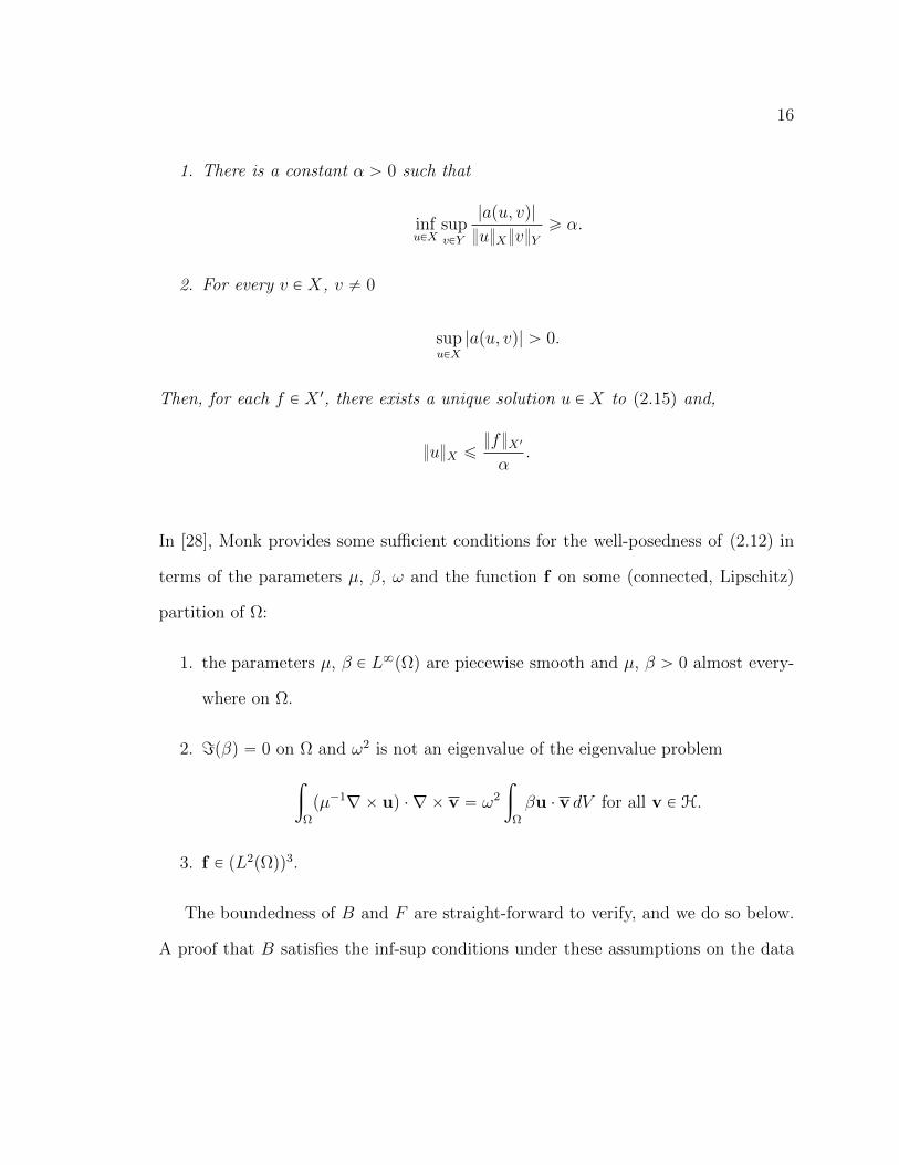
Table 4.6 Condition numbers of the stiffness matrices for V and W (Exam-
ple 2). . . . . . . . . . . . . . . . . . . . . . . . . . . . . . . . . 71
Table 5.1 Numerical errors and effectivity indices of goal-oriented error es-
timator when β P t´102,´10,´1, 1, 10u (Example 1). . . . . . . 81
Table 5.2 Numerical errors and effectivity indices of global error estima-
tor in H-curl and energy norms when β P t´102,´10,´1, 1, 10u
(Example 1). . . . . . . . . . . . . . . . . . . . . . . . . . . . . 82
Table 5.3 Condition numbers of the stiffness matrices for V and W for
β P t´102,´10,´1, 1, 10u (Example 1). . . . . . . . . . . . . . . 84
Table 5.4 Numerical errors and effectivity indices of goal-oriented and global
estimates over Ω1,Ω2,Ω3, and Ωs (Example 2). . . . . . . . . . . 88
Table 5.5 Condition numbers of the stiffness matrices for V and W in each
choice of subdomains (Example 2). . . . . . . . . . . . . . . . . 90

vii
List of Figures
Figure 4.1 The initial mesh and its uniform refinements (Example 1). . . 56
Figure 4.2 Uniform Solutions (Exact Versus Approximate Solutions) (Ex-
ample 1). . . . . . . . . . . . . . . . . . . . . . . . . . . . . . . . . . 57
Figure 4.3 Convergence rate of the exact error in H-curl norm (red) and
energy norm (blue) (Example 1). . . . . . . . . . . . . . . . . . . . . 61
Figure 4.4 Effectivity indices of the error estimators in H-curl norm (red)
and energy norm (blue) (Example 1). . . . . . . . . . . . . . . . . . . 61
Figure 4.5 Condition numbers of the stiffness matrices for V (red) and W
(blue) (Example 1). . . . . . . . . . . . . . . . . . . . . . . . . . . . . 63
Figure 4.6 Coarse mesh and Adaptive Refinement Levels (Example 2). . . 65
Figure 4.7 Adaptive Solutions (Exact Versus Approximate Solutions) (Ex-
ample 2). . . . . . . . . . . . . . . . . . . . . . . . . . . . . . . . . . 66
Figure 4.8 Convergence rate of the exact error in H-curl norm (red) and
energy norm (blue) (Example 2). . . . . . . . . . . . . . . . . . . . . 70
Figure 4.9 Effectivity indices of the error estimators in H-curl norm (red)
and energy norm (blue) (Example 2). . . . . . . . . . . . . . . . . . . 70
Figure 4.10 Condition numbers of the stiffness matrices for V (red) and W
(blue) (Example 2). . . . . . . . . . . . . . . . . . . . . . . . . . . . . 72
Figure 5.1 The subdomain Ωs of the domain Ω (Example 1). . . . . . . . 78
Figure 5.2 Adapted meshes, intermediate and final, to control Gpuq in Ωs
when β “ 1 (Example 1). . . . . . . . . . . . . . . . . . . . . . . . . . 79
Figure 5.3 Approximate Dual Solutions for intermediate and final meshes
for β “ 1 (Example 1). . . . . . . . . . . . . . . . . . . . . . . . . . . 79
Figure 5.4 Error estimators using the global error (GB) and goal-oriented
(GO) adaptivity strategy (Example 1). . . . . . . . . . . . . . . . . . 83
Figure 5.5 Effectivity indices using the global error (GB) and goal-oriented
(GO) adaptivity strategy (Example 1). . . . . . . . . . . . . . . . . . 83
Figure 5.6 Condition numbers of the stiffness matrices for V (red) and W
(blue) (Example 1). . . . . . . . . . . . . . . . . . . . . . . . . . . . . 85
Figure 5.7 The subdomain Ωs of the domain Ω (Example 2). . . . . . . . 86

viii
Figure 5.8 The final mesh refinement over each subdomain separately and
over all subdomains (Example 2). . . . . . . . . . . . . . . . . . . . . 87
Figure 5.9 Error estimators using the global error (GB) and goal-oriented
(GO) adaptivity strategy (Example 2). . . . . . . . . . . . . . . . . . 89
Figure 5.10 Effectivity indices using the global error (GB) and goal-oriented
(GO) adaptivity strategy (Example 2). . . . . . . . . . . . . . . . . . 89
Figure 5.11 Condition numbers of the stiffness matrices for V (red) and W
(blue) (Example 2). . . . . . . . . . . . . . . . . . . . . . . . . . . . . 91

1
Chapter 1
Introduction
Maxwell’s equations describe how electric charges and electric currents create electric
and magnetic fields, and how these fields propagate and influence each other. They
provide a mathematical model for many recent technologies, such as power gener-
ation, electric motors, wireless communication, lenses, radar etc. Electromagnetic
geophysics, more specifically the (inverse) problem of determining a realistic con-
ductivity/resistivity model of the earth near the surface (e.g. air/earth interface or
ocean/earth interface) from a series of experiments in which known sources are used
to generate the EM fields, and responses are measured at an array of locations, will
provide motivation for some of the choices in our development.
The use of finite element methods to approximate solutions of Maxwell’s equa-
tions goes back to at least 1980 [29], when Nedelec introduced his now-famous “edge
elements”, which provide a natural discretization of functions in the space Hpcurl; Ωq
in which the variatonal form of Maxwell’s equations is typically posed. Having used
the Nedelec (edge) element discretization to compute an approximation of the electric
field (for example), it is natural to ask how well it approximates the true solution.
One often quantifies this discretization error in terms of global norm. A priori error
estimates describe the qualitative behavior of the error with respect to parameters
governing the discretization, such as the characteristic edge length in a tetrahedral
mesh. Although such qualitative estimates provide useful information, in practice one
often wants more quantitative estimates of error, both to determine whether or not a
discrete solution is “good enough”, and to indicate how to intelligently improve the
discrete solution if it is not. This is the realm of a posteriori error estimation, which

2
is the focus of our research.
For standard finite element discretization of PDEs modeling diffusion processes, a
posteriori error theory is a mature field, and there are many well-tested techniques on
the market. In contrast, a posteriori error theory for Maxwell’s equations (by Nedelec
elements), is much more recent, and there are relatively few techniques in use that are
both theoretically and empirically supported [5, 7, 8, 11, 19, 21, 22, 25, 30, 34, 36]. Our
work will provide provably efficient and reliable error estimates of discretization error
based on auxiliary subspace techniques for Nedelec (edge) element discretization of
Maxwell’s equations on tetrahedral meshes. Such methods have a long history in the
context of standard discretization of diffusion problems, where they are often called
hierarchical basis error estimators [1, 3, 13, 14, 37]. Such estimators are based on the
computation of an approximate error function ε « u ´ u (u P V is a given finite
element approximation of the solution u) in an auxiliary discrete space W satisfying
V XW “ t0u. The traditional analysis of hierarchical error estimators [2, 4], in case
the bilinear form B is an inner-product with induced “energy norm” |||v|||2 “ Bpv,vq,
makes use of a strong Cauchy inequality between the spaces V and W and a saturation
assumption to obtain upper and lower bounds on error norm u´ u, in terms of the
error estimate norm ε. Roughly speaking, the saturation assumption asserts that
u is (strictly) better approximated in the “enriched space” V ‘W than it is in V ,
and this perspective, though intuitive, often causes viable auxiliary spaces W to be
overlooked [18,20].
Although the saturation assumption is expected to hold in many cases, construct-
ing counter-examples it is not difficult for particular problems on particular meshes.
Furthermore, this kind of analysis cannot be readily applied for the more general
bilinear forms such as those (that are not inner-products) considered here; and, as

3
suggested above, may unnecessarily limit the types of spaces W in which the error
might be approximated. The “saturation assumption approach” was taken in [5] to
derive a hierarchical basis error estimator for Maxwell’s equations, though it appears
that their work has not been pursued further. In this study we will take a different
approach, to obtain error bounds under weaker (and verifiable) assumptions, using
different spaces than in [5] . The principle of this approach is to replace the saturation
assumption by “residual oscillation”, which appears explicitly in the reliability bound
of the error as a computable quantity. The proof of this inequality depends primarily
on the choice of the space W in which the error indicator lies. We will also show that
the matrix of the auxiliary problem for computing the approximate error function in
W is spectrally equivalent to its diagonal, and therefore much simpler to work with
than the matrix for the original problem. Having established that the estimator is
efficient and reliable, and computationally feasible, we will extend the approach to
treat functional measures of error.
The rest of this thesis is organized as follows. In Chapter 2 we describe Maxwell’s
equations and introduce the strong and weak formulations. Also, at the end of this
chapter, we will briefly discuss assumptions that guarantee existence and uniqueness
of the weak form. The material in this chapter is standard and is presented here
to make our work more self-contained. The suitable finite elements of the Sobolev
space Hpcurl; Ωq, needed for discretizing the Maxwell system, will be presented in
Chapter 3. First, we will define the classical finite element spaces (FE spaces) for
the weak formulation, and then we will introduce the discrete variational problem.
In Chapter 4, we will introduce our key error estimation results, and will pursue the
analysis of our approach theoretically and empirically. We will show that the estimate
of the error is provably reliable and efficient, and the cost of computing such error

4
estimates is reasonable and not much expensive. Later in this chapter, we support
our arguments by numerical experiments. Lastly, in Chapter 5, we will present a new
approach in a posteriori error estimation, called Goal-oriented error estimation, in
which the numerical error of finite element approximations is estimated in terms of
quantities of interest rather than the classical global H-curl or energy norm. These
so-called quantities of interest are characterized by linear functionals on the space
of functions to where the solution belongs. We end this chapter with numerical
experiments which illustrate that the error in the goal functional is estimated very
precisely and can be reduced rapidly by applying the adaptive algorithm.

5
Chapter 2
Maxwell’s Equations: Strong and weak formulations, well-posedness
In this chapter we will describe Maxwell’s equations and introduce the strong form
(curl-curl problem) of these equations, which will be our starting point for the weak
formulation. Also, at the end of this chapter, we will briefly discuss assumptions that
guarantee existence and uniqueness of the weak form. The material in this chapter
is standard [28] and is presented here to make our work more self-contained, and to
introduce some key notation and terminology.
2.1 Maxwell’s equations
Maxwell’s equations are a set of four equations that describe how electric charges
and electric currents act as sources for electric and magnetic fields. Further, they
describe how these fields propagate and influence each other. Maxwell’s equations
state that the field variables and sources are related by the following equations which
apply throughout the region of space in R3 occupied by the electromagnetic field:
BBBt`∇ˆ E “ 0, (2.1a)
∇ ¨D “ ρ, (2.1b)
BDBt´∇ˆH “ ´J , (2.1c)
∇ ¨ B “ 0, (2.1d)
where
E= electric field,
H= magnetic field,

6
D= electric displacement,
B= magnetic induction,
ρ=electric charge density,
J=electric current density.
Equation (2.1a) is called Faraday’s law of induction, relating an electric field to a time-
varying magnetic flux. The divergence condition (2.1b) is Gauss’s law and gives the
effect of the charge density on the electric displacement. The next equation, (2.1c), is
Ampere’s law relating magnetic fields and currents, which was extended by Maxwell to
include induction of a magnetic field by a time-varying electric displacement. Finally,
equation (2.1d) is Coulomb’s law for magnetic flux, expressing the absence of isolated
magnetic charges.
In this work, we only consider the classical time-harmonic problem. For a detailed
overview of the investigation and derivation of this problem, we refer to [28].
2.2 Time-harmonic Maxwell’s equations
Assume the vector fields E , D, H, and B are periodic in time such that we can apply
Fourier transform in time, i.e. of the form
X px, tq “ <`
e´iωtXpxq˘
. (2.2)
The partial derivative to t will become a multiplication, e.g., BtX “ ´iωX . Here ω is
a positive constant called the frequency. To stay consistent we assume also the charge
density ρ, as well as the current density J to be of the form (2.2).

7
Under this assumption on the principle variables in (2.1), one obtains the time-
harmonic Maxwell equations,
´iωB`∇ˆ E “ 0, (2.3a)
∇ ¨D “ ρ, (2.3b)
´iωD´∇ˆH “ ´J, (2.3c)
∇ ¨B “ 0. (2.3d)
The electric and magnetic flux densities D, B are related to the field intensities
E, H via the so-called constitutive relations,
D “ εE and B “ µH, (2.4)
where ε is the permittivity and µ is the permeability. Furthermore, in conducting
materials the electric field induces a conduction current, which is given by Ohm’s law
J “ σE` Ja (2.5)
where σ is called the conductivity and is a non-negative function of position. The
vector function Ja describes the applied current density. In a vacuum (free space),
the permeability, the permittivity and conductivity are,
µ0 “ 4π ˆ 10´7V spAmq, ε0 “ 8.854ˆ 10´12F m, and σ0 “ 0.
The free space permeability and permittivity are further connected by c0 “ 1?ε0µ0,
where c0 « 2.998ˆ 108ms is the free space speed of light.

8
Using the constitutive relations in (2.4) and (2.5), we can obtain Maxwell’s Equa-
tions with only electric and magnetic fields:
∇ˆ E´ iωµH “ 0, (2.6a)
∇ˆH` piωε´ σqE “ Ja, (2.6b)
∇ ¨ pεEq “ ρ, (2.6c)
∇ ¨ pµHq “ 0. (2.6d)
Using (2.6a) to eliminate H from (2.6b) yields
∇ˆˆ
1
iωµ∇ˆ E
˙
` piωε´ σqE “ Ja. (2.7)
Usually, one writes this equation in a slightly different way by introducing the dimen-
sionless, relative permittivity and permeability by
µr “µ
µ0
, εr “β
ε0, β “ ε`
iσ
ω.
Then equation (2.7) takes the form
∇ˆ`
µ´1r ∇ˆ E
˘
´ κ2εrE “ iωµ0Ja, (2.8)
where the wavenumber κ “ ω?µ0ε0. We shall generally use (2.8) in this thesis.
2.3 Strong Form (curl-curl problem)
Let Ω Ă R3 be a bounded and Lipschitz domain with connected boundary BΩ and
unit outward normal n. We consider solving the classical time-harmonic Maxwell’s
equations subject to a perfect conducting boundary condition as follows:
∇ˆ pµ´1∇ˆ uq ´ ω2βu “ f in Ω , uˆ n “ 0 on BΩ , (2.9)

9
where u “ E is the time-harmonic electric field corresponding to a given current
density f “ iωJa, β “ ε0εr and µ “ µrµ0. Although we have chosen homogeneous
Dirichlet boundary conditions in (2.9), and will focus on this case in our work, some
of our results can easily be generalized to other types of boundary conditions.
2.4 Variational Framework
In this section we derive a variational (weak) formulation of the curl-curl problem
(2.9). In order to pose this variational form, we must first define appropriate function
spaces for the problem under consideration.
2.4.1 Notation
The gradient of a scalar-valued function of three variables q “ pq1, q2, q3q is given by
grad q “ ∇q “ˆ
Bq
Bq1
,Bq
Bq2
,Bq
Bq3
˙
.
For a vector v “ pv1, v2, v3q the formulas for the divergence and curl are
div v “ ∇ ¨ v “ Bv1
Bx`Bv2
By`Bv3
Bz,
curl v “ ∇ˆ v “
ˆ
Bv3
By´Bv2
Bz,Bv1
Bz´Bv3
Bx,Bv2
Bx´Bv1
By
˙
.
2.4.2 Function Spaces
The following function spaces will turn out to provide a natural setting for the inves-
tigation of the PDEs discussed above and ensure that all expressions in variational
form are well-defined.

10
Definition 2.1 (Function Spaces). We define the spaces
L2pΩq “
"
u :
ż
Ω
u2 dV ă 8
*
,
H1pΩq “ tp P L2
pΩq : ∇p P rL2pΩqs3u,
Hpcurl; Ωq “ tu P rL2pΩqs3 : ∇ˆ u P rL2
pΩqs3u,
Hpdiv; Ωq “ tp P rL2pΩqs3 : ∇ ¨ p P rL2
pΩqs3u,
and the corresponding norms and semi-norms
uL2pΩq “
ˆż
Ω
|u|2 dV
˙12
,
pH1pΩq “
´
p2L2pΩq ` ∇p2L2pΩq
¯12
, |p|H1pΩq “ ∇pL2pΩq,
uHpcurl;Ωq “
´
u2L2pΩq ` ∇ˆ u2L2pΩq
¯12
, |u|Hpcurl;Ωq “ ∇ˆ uL2pΩq,
pHpdiv;Ωq “
´
p2L2pΩq ` ∇ ¨ p2L2pΩq
¯12
, |p|Hpdiv;Ωq “ ∇ ¨ pL2pΩq.
All the above spaces are Hilbert spaces when equipped with the corresponding
scalar products defined by,
pu, vqL2pΩq “
ż
Ω
uv dV ,
pp, qqH1pΩq “
ż
Ω
∇p ¨∇q dV `ż
Ω
pq dV ,
pu,vqHpcurl;Ωq “
ż
Ω
p∇ˆ uq ¨ p∇ˆ vq dV `
ż
Ω
u ¨ v dV ,
pp,qqHpdiv;Ωq “
ż
Ω
p∇ ¨ pqp∇ ¨ qq dV `ż
Ω
p ¨ q dV .
Over-bar here (e.g. v) denotes complex conjugation. The relation between the func-
tional spaces through their differential operators can be summarized in the de Rham
diagram
H1pΩq
∇ÝÝÝÝÝÑ Hpcurl; Ωq
∇ˆÝÝÝÝÝÝÑ Hpdiv; Ωq
∇¨ÝÝÝÝÝÑ L2pΩq. (2.10)

11
From the point of view of Maxwell’s equations the space Hpcurl; Ωq is of central
importance since it corresponds to the space of finite-energy solutions.
2.4.3 Traces, Boundary Conditions and Variational Formulation
If Hpcurl; Ωq is to be used as the energy space for Maxwell’s equations, then tangential
trace of functions in this space must be well-defined [9, 10, 28]. To show that they
are, we first define boundary trace operators for smooth functions u P C8pΩq and
u P rC8pΩqs3:
γ0puq “ u|BΩ , γtpuq “ nˆ u|BΩ , γT puq “ pnˆ u|BΩq ˆ n.
It is well-known that γ0 can be continuously extended to a bounded linear operator
on H1pΩq, and this fact is used to define the trace space H12pBΩq, and its norm
H12pBΩq “ γ0pH
1pΩqq , vH12pBΩq “ inf
wPH1pΩqγ0pwq“v
wH1pΩq .
We define H´12pBΩq ““
H12pBΩq‰1
, the dual space of H12pBΩq (see Section 2.4.4).
Similarly, the tangential traces γt and γT can be continuously extended to bounded
linear operators on Hpcurl; Ωq, as discussed below.
Lemma 2.2. (Integration by Parts). The tangential trace operator γt is a bounded
linear operator from Hpcurl; Ωq into rH´12pBΩqs3, and it holdsż
Ω
p∇ˆ uq ¨ v dV ´
ż
Ω
u ¨ p∇ˆ vq dV “
ż
BΩ
γtpuq ¨ v ds (2.11)
for any u P Hpcurl; Ωq and v P rH1pΩqs3
Proof of this lemma can be found in [10].
Remark 2.3. The trace γt from Hpcurl; Ωq into rH´12pBΩqs3 is not surjective since
in (2.11) rH´12pBΩqs3 contains vectors that are not tangential to BΩ. The correct
space of the trace is examined in the next theorem.

12
Define a Banach space
Y pBΩq “ tf P rH´12pBΩqs3| there exists u P Hpcurl; Ωq such that γtpuq “ fu,
with norm given by
fY pBΩq “ infuPHpcurl;Ωqγtpuq“f
uHpcurl;Ωq .
Theorem 2.4. The following statements hold:
1. Y pBΩq is a Hilbert space.
2. γt : Hpcurl; Ωq Ñ Y pBΩq is surjective.
3. γT : Hpcurl; Ωq Ñ Y pBΩq1 is well-defined.
4. For any u,v P Hpcurl; Ωq, it holds
ż
Ω
p∇ˆ uq ¨ v dV ´
ż
Ω
u ¨ p∇ˆ vq dV “
ż
BΩ
γtpuq ¨ γT pvq ds .
Y pBΩq1 is the dual space of Y pBΩq (see Section 2.4.4). More details can be found
in [9, 10,28].
The space H0pcurl; Ωq is equal to the space of Hpcurl; Ωq functions with homoge-
nous tangential boundary conditions, and can be defined as
H0pcurl; Ωq “ tu P Hpcurl; Ωq : γtpuq “ 0 on BΩu .
Now we ready to derive the variational formulation of the strong problem (curl-curl
problem). We begin by multiplying problem (2.9) by a suitable “test” function v,
and integrating over Ω, to obtain
ż
Ω
∇ˆ pµ´1∇ˆ uq ¨ v dV ´
ż
Ω
ω2βu ¨ v dV “
ż
Ω
f ¨ v dV .

13
Using integration by parts to remove the outer curl operator µ´1∇ˆu from the first
integral, we obtain
ż
Ω
∇ˆ pµ´1∇ˆ uq ¨ v dV “
ż
Ω
pµ´1∇ˆ uq ¨ p∇ˆ vq dV `
ż
BΩ
γtpuq ¨ γT pvq dV .
Thus, we have
ż
Ω
pµ´1∇ˆ uq ¨ p∇ˆ vq dV ´
ż
Ω
ω2βu ¨ v dV “
ż
Ω
f ¨ v dV ´
ż
BΩ
γtpuq ¨ γT pvq ds .
By including our boundary conditions, we have the following weak form of the prob-
lem (2.9):
Find u P H such that
Bpu,vq “ F pvq for all v P H, (2.12)
where H “ H0pcurl; Ωq. The bilinear form B is given by
Bpu,vq “
ż
Ω
pµ´1∇ˆ uq ¨∇ˆ v ´ ω2βu ¨ v dV, (2.13)
and the linear form F pvq is given by
F pvq “
ż
Ω
f ¨ v dV, (2.14)
In later sections, we may “abuse” notation by dropping the boundary trace nota-
tion in favor of more familiar quantities that are well-defined when the functions are
sufficiently regular, e.g.
ż
BΩ
γtpuq ¨ γT pvq ds “
ż
BΩ
pnˆ uq ¨ pnˆ v ˆ nq ds
“
ż
BΩ
puˆ vq ¨ n ds “ ´
ż
BΩ
puˆ nq ¨ v ds.
Here we have used:

14
• the decomposition of v into its normal and tangential components, v “ pv ¨
nqn` nˆ v ˆ n,
• the fact nˆ u is orthogonal to n, so pnˆ uq ¨ pnˆ v ˆ nq “ nˆ u ¨ v,
• identities for reordering terms in a scalar triple product, nˆu ¨v “ uˆv ¨n “
´uˆ n ¨ v.
2.4.4 Abstract Well-posedness Results for Variational Problems
In this section, we briefly recall two key well-posedness results for variational problem
such as (2.12). Before stating these results, we need the following definitions.
Let X and Y denote Hilbert-spaces provided with the scalar products p¨, ¨qX ,
p¨, ¨qY , and the induced norms are denoted by ¨ X and ¨ Y .
Definition 2.5. Let X be a Hilbert space. A bounded linear functional on X is a
linear functional T such that there exists an M ą 0 where |T pxq| ď Mx for every
x P X. The dual space of X is denoted by X 1 and defined to be the space of bounded
linear functionals on X. If f P X 1 then the norm of f is
fX 1 “ supxPXx‰0
|fpxq|
xX.
We define the dual pairing x¨, ¨yX 1,X so that xf, xyX 1,X “ fpxq for all x P X and
f P X 1.
Definition 2.6. A mapping ap¨, ¨q : X ˆ Y Ñ C is called
1. a sesquilinear form if
• apα1u ` α2v, φq “ α1apu, φq ` α2apv, φq for all α1, α2 P C, u, v P X and
φ P Y ,

15
• apu, β1φ ` β2ψq “ β1apu, φq ` β2apu, ψq for all β1, β2 P C, u P X and
φ, ψ P Y ;
2. bounded if there is a constant C independent of u P X and φ P Y such that
|apu, φq| ď CuXφY for all u P X and φ P Y ;
3. coercive if there is a constant α ą 0 independent of u P X such that
|apu, uq| ě αu2X for all u P X.
We now consider the abstract variational problem: Find u P X such that
apu, vq “ fpvq for all v P X, (2.15)
where f P X 1 is a given linear functional and ap¨, ¨q is a bounded coercive sesquilinear
form on X ˆ X. The following lemma guarantees the existence and uniqueness of
this variational problem.
Lemma 2.7. (Lax-Milgram) Suppose a : X ˆ X Ñ C is a bounded and coercive
sesquilinear form. Then for each f P X 1 there exists a unique solution u P X to (2.15),
and
uX ďfX 1
α.
In the problem that we consider in this study, the presence of the term ´ω2βu ¨v
in Bpu,vq typically means that it is not coercive on H, so the Lax-Milgram lemma is
not sufficient to establish well-posedness of (2.12). To counter this problem, we need
a further generalization of Max-Milgram lemma.
Theorem 2.8. (Generalized Lax-Milgram Lemma) Let ap¨, ¨q : X ˆ Y Ñ C be a
bounded sesquilinear form which has the following properties:
16
1. There is a constant α ą 0 such that
infuPX
supvPY
|apu, vq|
uXvYě α.
2. For every v P X, v ‰ 0
supuPX
|apu, vq| ą 0.
Then, for each f P X 1, there exists a unique solution u P X to (2.15) and,
uX ďfX 1
α.
In [28], Monk provides some sufficient conditions for the well-posedness of (2.12) in
terms of the parameters µ, β, ω and the function f on some (connected, Lipschitz)
partition of Ω:
1. the parameters µ, β P L8pΩq are piecewise smooth and µ, β ą 0 almost every-
where on Ω.
2. =pβq “ 0 on Ω and ω2 is not an eigenvalue of the eigenvalue problem
ż
Ω
pµ´1∇ˆ uq ¨∇ˆ v “ ω2
ż
Ω
βu ¨ v dV for all v P H.
3. f P pL2pΩqq3.
The boundedness of B and F are straight-forward to verify, and we do so below.
A proof that B satisfies the inf-sup conditions under these assumptions on the data

17
is given in [28].
|Bpu,vq| ď µ´1L8pΩq∇ˆ uL2pΩq∇ˆ vL2pΩq ` ω
2βL8pΩquL2pΩqvL2pΩq,
ď maxtµ´1L8pΩq, ω
2βL8pΩqu
¨
˚
˝
∇ˆ uL2pΩq
uL2pΩq
˛
‹
‚
¨
¨
˚
˝
∇ˆ vL2pΩq
vL2pΩq
˛
‹
‚
,
ďM´
u2L2pΩq ` ∇ˆ u2L2pΩq
¯12 ´
v2L2pΩq ` ∇ˆ v2L2pΩq
¯12
,
“MuHpcurl;ΩqvHpcurl;Ωq.
where M “ maxtµ´1L8pΩq, ω2βL8pΩqu.
Again using the Cauchy-Schwarz inequality with F pvq, we have
|F pvq| ď fL2pΩqvL2pΩq ď fL2pΩqvHpcurl;Ωq.
Remark 2.9. From here onwards we shall absorb the constants ω and β in one
constant, and we will call it β again.
Remark 2.10. In our particular case, the regular inf-sup conditions is defined by
infuPHu‰0
supvPHv‰0
|Bpu,vq|
uHvHě α. (2.16)
for some constant α ą 0.

18
Chapter 3
Finite Elements for Maxwell’s Equations
From the previous chapter, we saw that the Sobolev space Hpcurl; Ωq plays a central
role in the variational theory of Maxwell’s equations. Thus we need suitable finite
elements in this space for discretizing the Maxwell system. First, we will shortly
recall the main ingredients for the finite element method (FEM), and then define the
classical finite element spaces (FE spaces) for (2.12) , namely the Nedelec elements
of first kind. lastly, we will introduce the discrete variational problem.
3.1 Triangulation and Finite Element Spaces
The first step in applying finite elements methods is to generate a finite element
triangulation (mesh) covering the domain Ω. Recall that Ω is a bounded polyhedral
domain with Lipschitz boundary.
Definition 3.1. A triangulation (mesh) T is a finite non-overlapping subdivision of
Ω into elements Ti of simple geometry. A triangulation is called regular, if
1. the elements are non-overlapping, i.e.
interiorpTiq X interiorpTjq “ H for i ‰ j;
2. the triangulation T is a covering of Ω, i.e.
ď
TiPT
Ti “ Ω;
3. the intersection Ti X Tj of two different elements (i ‰ j) is either empty, or a
vertex, or an edge or a face of both elements;

19
4. each T P T is a Lipschitz domain.
For each face F , we define the parameter hF such that
hF “ diameter of F ,
and for each element T , we define the parameter hT such that
hT “ diameter of T (diameter of the smallest sphere containing T ),
then h “ maxTPT hT so that the index h denotes the maximum diameter of the ele-
ments T P T.
We will frequently use the following notations
the set of vertices V “ tziu, the set of edges E “ teiu,
the set of faces F “ tFiu, the set of elements T “ tTiu.
The sets of the interior faces and interior edges are denoted by FI and EI , respectively,
and the (local) sets of vertices, edges, and faces belonging to the element T are denoted
by VT , ET , and FT .
In this study, we consider a tetrahedral mesh of a polyhedral domain. Thus each
T P T is a tetrahedron with vertices z1, z2, z3, z4 P V.
After having the most characteristic aspect of the finite element method, the
triangulation, we can define a finite element. Following the classical approach of
Ciarlet in [12], the classical definition is the following:
Definition 3.2 (Finite Element). The triple (T,PT ,ΣT ) is a finite element provided,
1. T Ă Rn is a compact set with non-empty interior and (piecewise smooth) Lips-
chitz boundary,
2. PT is a finite-dimensional space of functions on T , with dimpPT q “ k.

20
3. The functionals ΣT “ tfi,T uki“1 are a basis for PT . They are called the (local)
degrees of freedom of the finite element.
3.2 Polynomial spaces and Nedelec Space
Local FE spaces are usually spanned by polynomial functions. Let us start by defining
basic polynomial spaces that will be needed in the forthcoming definitions. We define
Pp to be the polynomials of (total) degree at most p in x “ px1, x2, x3q and Pp to be
the subset of Pp consisting of homogeneous polynomials of degree precisely p. Recall
that a polynomial v is called homogeneous of degree p when vpαxq “ αpvpxq for any
constant α—in other words, all monomial terms in v have degree p. It holds that
dimPp “ˆ
p` 3
3
˙
, dim Pp “ˆ
p` 2
2
˙
. (3.1)
More generally, if these polynomials had been in n variables instead of 3, then 3 would
be replaced by n and 2 by n´ 1 in (3.1). A nice algebraic property of Pp is that
v “ px ¨∇vqp for v P Pp , so p∇v “ 0 ùñ v “ 0q for v P Pp . (3.2)
We also see that ∇v P rPp´1s3 for v P Pp.
We now define a space Sp and give its dimension,
Sp “ tv P rPps3 : x ¨ v “ 0u , dim Sp “ 3 dim Pp ´ dim Pp`1 “ ppp` 2q . (3.3)
Since v P Pp`1 if and only if v “ x ¨v for some v P rPps3 (in fact v “ px ¨∇vqpp` 1q),
the constraint x ¨ v “ 0 in the definition of Sp removes a subspace of dimension
dim Pp`1 from rPps3; this explains the formula for dim Sp. It also follows from the
discussion above that Sp is gradient free, in the sense that v “ ∇v P Sp if and only if
v “ 0.

21
Nedelec spaces are perhaps the most widely used finite element spaces in compu-
tational electromagnetic. For discretizing the variational problem (2.12) we use the
Hpcurl,Ωq-conforming finite element space introduced by Nedelec [29]. For any given
conforming tetrahedral triangulation T of Ω, the local p-order Nedelec space of the
first-kind, with its dimension, is defined by
Rp “ rPp´1s3‘ Sp , dimRp “ ppp` 2qpp` 3q2 . (3.4)
A key algebraic property of Rp is that
rPps3 “ Rp ‘∇Pp`1 . (3.5)
Applying (3.5) to (3.4), we have a decomposition of Rp into a gradient space and a
gradient-free space,
Rp “
´
∇P1 ‘ ¨ ¨ ¨ ‘∇Pp¯
‘ pS1 ‘ ¨ ¨ ¨ ‘ Spq
“ ∇Pp ‘ pS1 ‘ ¨ ¨ ¨ ‘ Spq “ RGp ‘ RF
p .
The dimensions of these spaces are
dimRGp “
pÿ
k“1
dim∇Pk “pÿ
k“1
dim Pk “pÿ
k“1
ˆ
k ` 2
2
˙
“ ppp2` 6p` 11q6 , (3.6)
dimRFp “
pÿ
k“1
dim Sk “
pÿ
k“1
kpk ` 2q “ ppp` 1qp2p` 7q6 . (3.7)
We also note that dimRGp “ dim∇Pp “ dimPp´ 1. For reference, we include a table
of these dimensions for a few small values of p in Table 3.1.
Now we can define the curl conforming element on a general tetrahedron T and
describe how v P VppT q is uniquely determined by specifying certain moments on its
edges, faces and volume.
Definition 3.3. The curl-conforming finite element of Nedelec is defined by:

22
p dimRp dimRGp dimRF
p dimV Ep pT q dimV F
p pT q dimV Tp pT q
1 6 3 3 6 0 0
2 20 9 11 12 8 0
3 45 19 26 18 24 3
Table 3.1: The dimensions of VppT q “ Rp and its gradient and gradient-free subspaces
RGp and RF
p , together with those of the edge, face and volume subspaces V Ep pT q,
V Fp pT q, V
Tp pT q, for small p.
• T is a tetrahedron,
• VppT q “ Rp,
• The degrees of freedom are of three types associated with edges e of T , faces F
of T and T itself. We denote by t a unit vector in the direction of the edge e.
There are three different degrees of freedom:
1. the first set is associated with edges of the element:
Mepvq “
"ż
e
v ¨ t q ds for all q P Pp´1peq and e P ET
*
; (3.8)
2. the second set is associated with faces of the element:
MF pvq “
"ż
Fk
pv ˆ nkq ¨ q dA for all q P rPp´2pF qs3 and F P F
*
; (3.9)
3. the last set is associated with the volume:
MT pvq “
"ż
T
v ¨ q dV for all q P rPp´3pT qs3
*
. (3.10)
Then ΣT “Mepvq YMF pvq YMT pvq.
In light of this, we decompose VppT q as VppT q “ V Ep pT q ‘ V
Fp pT q ‘ V
Tp pT q, where
all functions in V Tp pT q have vanishing face and edge moments, and V F
p pT q Ă VppT qa

23
V Tp pT q consists of those functions which have vanishing edge moments. We refer to
V Ep pT q as the edge space, V F
p pT q as the face space, and V Tp pT q as the volume space.
3.3 Barycentric Coordinates on the Tetrahedron
Particularly important polynomials in P1 are the barycentric coordinates, defined
below. It is useful to replace the Euclidean coordinates of the point x P R3 by
barycentric coordinates denoted by λi “ λipxq with respect to the four vertices zi P
VT , and many important finite elements can be expressed in terms of these coordinates
as we will do.
Definition 3.4 (Barycentric Coordinates). Let zi, i “ 1, ¨ ¨ ¨ , 4, be the vertices of a
non-degenerate tetrahedron T Ă R3, we define the following:
• Six edges eij, 1 ď i ă j ď 4, between vertices zi and zj, and the unit tangent
vector tij “ pzj ´ ziq|zj ´ zi|.
• Four faces Fk, 1 ď k ď 4, with Fk opposite vertex zk, and outward unit normal
nk. We define the distance between zk and the plane containing Fk as αk, and
note that αk “ 3|T ||Fk|.
Then the barycentric coordinate function λipxq is the unique polynomial function in
P1 such that λipxjq “ δij, 1 ď j ď 4. A formula for λipxjq is given by
λipxq “ 1´px´ ziq ¨ ni
αi“ δij `∇λi ¨ px´ zjq .

24
An alternate formulation is found by solving the system of equations
4ÿ
k“1
λkpxqzk “ x ,4ÿ
k“1
λkpxq “ 1 ðñ
¨
˚
˝
1 1 1 1
z1 z2 z3 z4
˛
‹
‚
looooooooooomooooooooooon
M
¨
˚
˚
˚
˚
˚
˚
˚
˝
λ1pxq
λ2pxq
λ3pxq
λ4pxq
˛
‹
‹
‹
‹
‹
‹
‹
‚
“
¨
˚
˝
1
x
˛
‹
‚
.
Cramer’s rule can be used to determine a generic formula for each coordinate, with
detpMq “ ˘6|T |. The assumption that the elements are non-degenerate implies that
|T | ‰ 0.
3.4 Basis for Local Space VppT q “ Rp
The decomposition VppT q “ V Ep pT q ‘ V F
p pT q ‘ V Tp pT q suggests that a natural basis
for VppT q would also be decomposed in this manner. Two references in which this is
accomplished in terms of barycentric coordinates are [17,35]. We essentially reproduce
the basis given in [17] where the basis for Nedelec spaces are presented of any order
in any space dimension. The main feature of this basis is that it is expressed just
in terms of the barycentric coordinates of the simplex. Table 3.2 shows the basis for
Nedelec space on a tetrahedron T in barycentric coordinates for order 1 ď p ď 3.
We take the vertices of T to be indexed by pi, j, k, `q, or p1, 2, 3, 4q if all four indices
appear in a given expression.
3.5 Global Spaces, Dimension and Bases
Given a conforming tetrahedral partition T of Ω, we define the global approximation
space Vp as:
Vp “ tv P H : v|T P VppT q for all T P Tu. (3.11)

25
p V Ep pT q on eij V F
p pT q on F` “ Fijk V Tp pT q
1 λi∇λj ´ λj∇λi2 λipλi∇λj ´ λj∇λiq λiλj∇λk ´ λjλk∇λi
λjpλi∇λj ´ λj∇λiq λjλk∇λi ´ λkλi∇λj3 λ2
i pλi∇λj ´ λj∇λiq λipλiλj∇λk ´ λjλk∇λiq λ1λ2λ3∇λ4 ´ λ2λ3λ4∇λ1
λiλjpλi∇λj ´ λj∇λiq λjpλiλj∇λk ´ λjλk∇λiq λ2λ3λ4∇λ1 ´ λ3λ4λ1∇λ2
λ2jpλi∇λj ´ λj∇λiq λkpλiλj∇λk ´ λjλk∇λiq λ3λ4λ1∇λ2 ´ λ4λ1λ2∇λ3
λipλjλk∇λi ´ λkλi∇λjqλjpλjλk∇λi ´ λkλi∇λjqλkpλjλk∇λi ´ λkλi∇λjq
Table 3.2: Bases given in [17] (up to sign) for VppT q in terms of barycentric coordi-
nates, p ď 3.
As suggested by the discussion of degrees of freedom above, the dimensions of this
space is
dimVp “ p#E` ppp´ 1q#F ` 0.5ppp´ 1qpp´ 2q#T. (3.12)
For a piecewise polynomial to be in Hpcurlq, it need only have a continuous tan-
gential component across all interior faces in the mesh. It is natural to again split the
space Vp as Vp “ V Ep ‘V
Fp ‘V
Tp , and consider bases for each part. For each T P T we
choose our global volume basis functions associated with T to coincide with the local
volume basis functions on T , extending the local functions by 0 outside T . Similarly,
for each face F P FI we choose our global face basis functions associated with F so
that they coincide with the local face basis functions on the pair of tetrahedra sharing
F , and vanish outside of this pair. Finally, for each edge e P EI we choose our global
edge basis functions so that they coincide with local edge basis functions given above
on the ring of tetrahedra sharing e, and vanish outside this ring. In this study, we
shall always consider the lowest-order (p “ 1) Nedelec space Vp for approximating the

26
solution of (2.12), and we define V “ V1.
3.6 The discrete variational problem
The infinite-dimensional space H is now replaced by a sequence of finite-dimensional
spaces V , which yields the discrete variational problem of (2.12): Find u P V such
that
Bpu,vq “ F pvq for all v P V . (3.13)
The continuity on V is inherited from the variational problem on H . The gen-
eralized Lax-Milgram theorem 2.8 can be applied to the discrete formulation so that
the two conditions:
1. There is a constant α ą 0 such that
infuPVu‰0
supvPVv‰0
|Bpu,vq|
uV vVě α. (3.14)
2. For every v P V , v ‰ 0
supuPV
|Bpu,vq| ą 0.
imply existence of a unique solution. The former condition (3.14) is called discrete
inf-sup condition. A fundamental property, which is called the Galerkin orthogonality,
can be obtained by subtracting (3.13) form (2.12), so that
Bpu´ u,vq “ Bpu,vq ´Bpu,vq “ F pvq ´ F pvq “ 0, for all v P V . (3.15)
Lemma 3.5 (Cea). Suppose V is a finite-dimensional subspace of H. Suppose Bp¨, ¨q
is continuous with bound C, and Bp¨, ¨q fulfill the discrete inf-sup condition (3.14).
Let u P V solve the discrete problem (3.13). Then, the following error estimate holds:
u´ uHpcurl;Ωq ď
ˆ
1`C
α
˙
u´ vHpcurl;Ωq

27
Proof. Galerkin orthogonality implies Bpu,wq “ Bpu,wq for all w P V . For any
v P V it holds
u´ uHpcurl;Ωq ď u´ vHpcurl;Ωq ` v ´ uHpcurl;Ωq
Combining the discrete inf-sup condition (3.14), the Galerkin orthogonality and the
continuity of B yields
u´ uHpcurl;Ωq ď u´ vHpcurl;Ωq ` α´1 sup
wPVw‰0
Bpv ´ u,wq
wHpcurl;Ωq
“ u´ vHpcurl;Ωq ` α´1 sup
wPVw‰0
Bpv ´ u,wq
wHpcurl;Ωq
ď u´ vHpcurl;Ωq ` α´1 sup
wPVw‰0
Cv ´ uHpcurl;ΩqwHpcurl;Ωq
wHpcurl;Ωq
“
ˆ
1`C
α
˙
|u´ vHpcurl;Ωq.
3.7 The interpolant for V
Associated with the finite element T,Rp,ΣT is an interpolant. For a suitable smooth
function u P H, we define the interpolant on T , where T P T, to be the unique
function rTu P Rp such that
Mepu´ rTuq “
ż
e
pu´ rTuq ¨ t q ds “ 0 for all q P P0 on e of T.
The operator rTu : H Ñ Rp is referred to as the interpolation operator. The global
interpolant rhu P V is then defined element by element using rhu|T “ rTu for all
T P T. In this study, we shall always denote to rhu by u.
With our setting for the finite element method, it would be possible to show
Theorem 5.41 in [28], which provides a priori error estimates for the interpolant.

28
Here we only consider a special case of this theorem, for the general one and for the
proof see [28].
Theorem 3.6. Let T be a regular mesh on Ω. If u P rH1pΩqs3 and ∇ˆu P rH1pΩqs3,
then
u´ u2Hpcurl;Ωq ď Chpu2rH1pΩqs3 ` ∇ˆ u2rH1pΩqs3q
where C is a constant depending on the geometry of the domain and the mesh.

29
Chapter 4
A posteriori Error Estimation
Having used the Nedelec (edge) element discretization to compute an approximation
of the electric field (for example), it is natural to ask how well it approximates the
true solution. One often quantifies this discretization error in terms of global norm.
A priori error estimates describe the qualitative behavior of the error with respect
to parameters governing the discretization, such as the characteristic edge length in
a tetrahedral mesh. Although such qualitative estimates provide useful information,
in practice one often wants more quantitative estimates of error, both to determine
whether or not a discrete solution is “good enough”, and to indicate how to intelli-
gently improve the discrete solution if it is not. This is the realm of a posteriori error
estimation, which is the focus of our research.
For standard finite element discretizations of PDEs modeling diffusion processes, a
posteriori error theory is a mature field, and there are many well-tested techniques on
the market. In contrast, a posteriori error theory for Maxwell’s equations (by Nedelec
elements), is much more recent, and there are relatively few techniques in use that
are both theoretically and empirically supported [5, 7, 8, 11,19,21,22,25,30,34,36].
4.1 Hierarchical Based Error Estimator
Our work will provide provably efficient and reliable error estimates of discretization
error based on auxiliary subspace techniques for Nedelec (edge) element discretization
of Maxwell’s equations on tetrahedral meshes. Such methods have a long history in
the context of standard discretizations of diffusion problems, where they are often

30
called hierarchical basis error estimators [1, 3, 13, 14, 37]. Such estimators are based
on the computation of an approximate error function ε « u´u (u P V is a given finite
element approximation of the solution u) in an auxiliary discrete space W satisfying
V XW “ t0u. The traditional analysis of hierarchical error estimators [2, 4], in case
the bilinear form B is an inner-product with induced “energy norm” |||v|||2 “ Bpv,vq,
makes use of a strong Cauchy inequality between the spaces V and W
|Bpv,wq| ď γ|||v||||||w||| for all v P V and w P W, where γ P p0, 1q,
and a saturation assumption
|||u´ u||| ď α|||u´ u||| for all u P H, u P V ‘W, and u P V, where α P p0, 1q,
to obtain upper and lower bounds on error norm u´u, in terms of the error estimate
norm as follows ε
|||ε||| ď |||u´ u||| ď|||ε|||
a
p1´ γ2qp1´ α2q.
Roughly speaking, the saturation assumption asserts that u is (strictly) better ap-
proximated in the “enriched space” V ‘ W than it is in V , and this perspective,
though intuitive, often causes viable auxiliary spaces W to be overlooked [18,20].
Although the saturation assumption is expected to hold in many cases, construct-
ing counter-examples it is not difficult for particular problems on particular meshes.
Furthermore, this kind of analysis cannot be readily applied for the more general
bilinear forms such as those (that are not inner-products) considered here; and, as
suggested above, may unnecessarily limit the types of spaces W in which the error
might be approximated. The “saturation assumption approach” was taken in [5] to
derive a hierarchical basis error estimator for Maxwell’s equations, though it appears
that their work has not been pursued further. In this study we will take a different

31
approach, to obtain error bounds under weaker (and verifiable) assumptions, using
different spaces than in [5] . The principle of this approach is to replace the saturation
assumption by “residual oscillation”, which appears explicitly in the reliability bound
of the error as a computable quantity.
4.2 Key Error Estimation Result
Given a finite dimensional supspace W of H such that V XW “ t0u, we consider the
error problem: Find ε P W such that
Bpε,vq “ F pvq ´Bpu,vqloooooooomoooooooon
Bpu´u,vq
for all v P W. (4.1)
If B is an inner-product, then ε is the corresponding orthogonal projection of the
error u´ u onto W . Even when B is not an inner-product, we may refer to ε as the
projection of u´ u onto W . Appropriate global and local norms of ε, e.g. εHpcurl;Ωq
and εHpcurl;T q, will be used to determine whether the discretization error is small
enough; and, if it is not, how it can be efficiently reduced. Clearly, the choice of
auxiliary (error) space W is crucial to the success of this approach, and we describe
below the motivations for our choice, and the type of theoretical results that we will
establish. As mentioned in the introduction, we must balance two objectives in our
choice of W :
1. The estimate εHpcurl;Ωq of u´ uHpcurl;Ωq should be provably reliable and effi-
cient.
2. The cost of computing ε P W should be reasonable, i.e., not more than, and
preferably much less than, that of computing u P V .
Having established (1) and (2), we will extend the approach to treat functional mea-
sures of error (in chapter 5).

32
The starting point of our analysis is the error identity in Proposition (4.1), which
follows directly from (2.12), (3.13), and (4.1). The oscillation term in our error
bound will come from Bpu´ u,v´ v´wq, so we investigate this term for guidance in
choosing W . Let F denote the faces of T and g “ v´ v´ w. Writing Bpu´ u,gq “
F pgq ´Bpu,gq as a sum of integrals over tetrahedra, and using integration-by-parts
on each of these integrals, we obtain,
Bpu´ u,gq “
ż
Ω
pf ` βuq ¨ g ´ pµ´1∇ˆ uq ¨∇ˆ g dV
“ÿ
TPT
ˆż
T
pf ` βu´∇ˆ pµ´1∇ˆ uqq ¨ g dV
`
ż
BT
pµ´1∇ˆ uq ¨ pg ˆ nq dA
˙
.
Proposition 4.1. for any v P H, v P V , and w P W , it holds that
Bpu´ u,vq “ Bpε, wq `Bpu´ u,v ´ v ´ wq,
where
Bpu´ u,gq “ F pgq ´Bpu,gq “ÿ
TPT
ż
T
RT ¨ g dV `ÿ
FPF
ż
F
rF ¨ pg ˆ nq dA.
and RT “ f ` βu ´ ∇ ˆ pµ´1∇ ˆ uq is the volumetric (strong) residual, and rF “
rµ´1∇ˆ usJ is the jump in the weighted curl µ´1∇ˆ u across the face F once a single
normal n is chosen.
Remark 4.2. If µ´1 is piecewise constant then rF ¨ pgˆnq will vanish when we make
a proper choice of g, and also ∇ˆ pµ´1∇ˆ uq “ 0 in RT .
With an appropriate choice of error space W (described in detail later), we obtain
our key error theorem,

33
Theorem 4.3. When h is sufficiently small, then there are constants k1 and k2
depending on the shape-regularity of T and problem data µ and β such that
k1εHpcurl;Ωq ď u´ uHpcurl;Ωq ď k2
`
εHpcurl;Ωq ` oscpR, r,Tq˘
(4.2)
where the residual oscillation is defined by
oscpR, r,Tq2 “ÿ
TPT
h2T infλTPR3
RT ´ λT 2L2pT q
`ÿ
FPF
hF infκFPR3
prF ´ κF q ˆ n2L2pF q.
(4.3)
Some justification of why might hope to prove such bounds is given in [18, 20],
where bounds of this type are proven for a different class of PDE.
The computation of ε requires the solution of a global system involving the stiffness
matrix associated with W . At first glance this would seem to rule out the approach
as too expensive for practical computations, but we argue herein that this is not the
case. In Sect. 4.5 we argue that the matrix associated with the computation of ε,
though larger than that associated with the computation of u, is much better condi-
tioned. More particularly, we will argue that this matrix is spectrally equivalent to
its diagonal, which is certainly not the case for the matrix associated with computing
u on V . Our key result in this regard is
Theorem 4.4. The global stiffness matrix for W is spectrally-equivalent to its diag-
onal.
4.3 Local and Global Error Space W
Choosing the error space W plays important role in our error estimation analysis.
In view of the structure of the term Bpu ´ u,v ´ v ´ wq in Proposition 4.1, it is
natural to consider an error space W that has degrees of freedom associated with each

34
tetrahedron and all (interior) faces in the mesh. We define such a space below, and
show some of its key properties that will be instrumental in the proofs of Theorems 4.3
and 4.4.
The corresponding global finite error space W and its dimensions are given by
W “ tv P H : v|T P VF
2 pT q ‘ VT
3 pT q for all T P Tu, (4.4)
dimW “ 2 #F ` 3 #T . (4.5)
We decompose W pT q as W pT q “ V F2 pT q ‘ V T
3 pT q, where all functions in V T3 pT q
have vanishing face and edge moments, and V F2 pT q consists of those functions which
have vanishing edge moments. We refer to V F2 pT q as the face space, and V T
3 pT q as
the volume space. This decomposition suggests that a natural basis for W pT q would
also be decomposed in this manner. The bases of W pT q are given in the Table 3.2.
So, any w P W pT q is uniquely decomposed as w “ w2 ` w3 with w2 P VF
2 pT q and
w3 P VT
3 pT q.
Remark 4.5. The auxiliary error space ĂW that used in [5] is defined as
ĂW “ tv P H : v|T P rV E2 pT q ‘ V
F2 pT q for all T P Tu,
dimĂW “ #E` 2 #F,
where rV E2 pT q “ V E
2 pT qaVE
1 pT q. In the linear system associated with our error space
W , we can locally eliminate degrees of freedom associated with each V T3 pT q, so our
global system really only needs to be as large as the twice the number of faces. In the
approach used in [5], such a reduction is not possible, so their systems associated with
ĂW are inherently larger and have a more complicated structure.
Lemma 4.6. If w P V F2 pT q ‘ V
T3 pT q satisfies ∇ˆw “ 0, then w “ 0.

35
Proof. Using Stoke’s Theorem and the Divergence Theorem, we see that for suffi-
ciently smooth w, g and g,¿
BF`
w ¨ t g ds “
ż
F`
∇ˆ pgwq ¨ n` dA “ż
F`
g p∇ˆw ¨ n`q ` pw ˆ n`q ¨∇g dA ,
ż
BT
pw ˆ nq ¨ g dA “
ż
T
∇ ¨ pg ˆwq dV “
ż
T
w ¨ p∇ˆ gq ´ g ¨ p∇ˆwq dV ,
where t is the unit tangent vector around BF` and n` is the outward unit normal to
face F`. From this we see that, if ∇ˆw “ 0, then¿
BF`
w ¨ t g ds “
ż
F`
pw ˆ n`q ¨∇g dA ,
ż
BT
pw ˆ nq ¨ g dA “
ż
T
w ¨ p∇ˆ gq dV .
Consider w P V F2 pT q and w P V T
3 pT q separately. For w P V Fp pT q, the edge moments
vanish, so we have,ż
F`
pw ˆ n`q ¨∇g dA “ 0
for g P Pp´1. When p “ 2, we obtain a full set of face degrees of freedom by choosing
g “ c ¨ x for arbitrary c P R3. Since all degrees of freedom vanish for w, we deduce
that w “ 0 when p “ 2.
For w P V Tp pT q the edge and face moments vanish, so we have
ż
T
w ¨ p∇ˆ gq dV “ 0
for g P rPp´2s3. When p “ 3 we obtain a full set of volume degrees of freedom by
choosing g “ pbz, cx, ayq for arbitrary pa, b, cq P R3. Since all degrees of freedom
vanish for w, we deduce that w “ 0 when p “ 3.
In this study, we will use W2pT q “ V F2 pT q and W3pT q “ V T
3 pT q.
Proposition 4.7. For any T P T and any w P W pT q, ∇ ˆ wL2pT q is a norm on
W pT q. Moreover, there are a scale-invariant constants c, C ą 0 such that
ch´1T wL2pT q ď ∇ˆwL2pT q ď Ch´1
T wL2pT q for all w P W pT q.

36
Proof. For any v,w P W pT q, let xv,wy defined by
xv,wy “
ż
T
p∇ˆ vq ¨ p∇ˆwq dV.
From this definition and from Lemma 4.6, we have xv,vy “ 0 if and only if v “ 0
and xαv, αvy “ |α|2xv,vy for any α P C. In other words, ∇ ˆ vL2pT q “ 0 ô v “ 0
and ∇ˆ pαvqL2pT q “ |α|∇ˆ vL2pT q. Considering v,w P W pT q, we have
∇ˆ pv `wq2L2pT q “ xv `w,v `wy “ xv,vy ` xw,wy ` xv,wy ` xw,vy
“ ∇ˆ v2L2pT q ` ∇ˆw2L2pT q ` 2<pxv,wyq
and using Cauchy-Schwarz inequality,
∇ˆ pv `wq2L2pT q ď ∇ˆ v2L2pT q ` ∇ˆw2L2pT q ` 2|xv,wy|
ď ∇ˆ v2L2pT q ` ∇ˆw2L2pT q ` 2a
xv,vyxw,wy
ď ∇ˆ v2L2pT q ` ∇ˆw2L2pT q ` 2∇ˆ vL2pT q∇ˆwL2pT q
“`
∇ˆ vL2pT q ` ∇ˆwL2pT q
˘2
Hence, ∇ ˆ pv ` wqL2pT q ď ∇ ˆ vL2pT q ` ∇ ˆ wL2pT q (triangle inequality).
Therefore ∇ˆ vL2pT q is a norm on W pT q.
Let T “ tx “ h´1T x : x P T u where T is a physical element with diampT q “ hT
and T is a reference element with diampT q “ 1. For each w : W pT q Ñ R, define
w : W pT q Ñ R by wpxq “ wphT xq “ wpxq. It is clear that
w2L2pT q “
ż
T
|wpxq|2 dV “
ż
T
|wpxq|2h3T dx “ h3
T w20,T, (4.6)
∇ˆw2L2pT q “
ż
T
|∇ˆwpxq|2 dV “
ż
T
h´2T |∇ˆ wpxq|2h3
T dx “ hT ∇ˆ w20,T.
(4.7)

37
W pT q is a finite dimensional vector space on T . ¨ 0,T and ∇ˆ¨0,T are both norms
on W pT q, so there are constants c, C such that
cw0,T ď ∇ˆ w0,T ď Cw0,T for all w P W pT q.
From (4.6) and (4.7), we have
ch´1T wL2pT q ď ∇ˆwL2pT q ď Ch´1
T wL2pT q
Proposition 4.8. Suppose that β is real on T and µ satisfies µ´1 ě m ą 0 on Ω for
some real m. Given T P T and w P W pT q, there is a constant σT ě m2 for which
BT pw,wq ě σT ∇ˆw2L2pT q when hT is sufficiently small.
Proof. Let BT pu,vq be the element-wise bilinear form for Bpu,vq. Then we have
BT pw,wq “
ż
T
µ´1T |∇ˆw|2 dV ´
ż
T
βT |w|2 dV
ě µ´1T ∇ˆw2L2pT q ´ βL8pT qw
2L2pT q dV .
From 4.7, we obtain
BT pw,wq ě µ´1T ∇ˆw2L2pT q ´ βL8pT qcTh
2T ∇ˆw2L2pT q
“ pµ´1T ´ βL8pT qcTh
2T q∇ˆw2L2pT q
“ σT ∇ˆw2L2pT q,
where σT “ µ´1T ´ βL8pT qcTh
2T . When hT is small enough, σT ě
µ´1T
2ě m
2ą 0.
4.4 Reliability Analysis
Before we prove Theorem 4.3, we need to establish several theorems and lemmas. We
will need the small domains (patches) associated with vertices and elements of the

38
mesh. The following definitions of patches will be useful in the following analysis.
For a given vertex z P V, we assign to it the patch Ωz “Ť
tT : z P BT u. Then we
define the domains
Ωz “ď
z1PΩz
Ωz1 and ΩT “ď
z1PTΩz1 .
containing the neighbor elements of neighbor elements of a vertex z and an element
T , respectively.
Theorem 4.9. [34, Theorem 1]. There exists an operator ΠE : H0pcurl; Ωq Ñ V
with the following properties: For every v P H0pcurl; Ωq there exists φ P H10 pΩq and
ψ P rH10 pΩqs
3 such that
v ´ ΠEv “ ψ `∇φ
The decomposition satisfies
h´1T φL2pT q ` ∇φL2pT q ď CvL2pΩT q
,
h´1T ψL2pT q ` ∇ψL2pT q ď C∇ˆ vL2pΩT q
.
The constant C depends only on the shape of the elements in the enlarged element
patch ΩT , but does not depend on the global shape of the domain Ω or the size of the
patch ΩT .
Lemma 4.10. Let v, φ and ψ satisfy the decomposition in Theorem 4.9. Then there
are scale-invariant constants C1 and C2 such that
(i) φL2pF q ď C1h12T vL2pΩT q
,
(ii) ψL2pF q ď C2h12T ∇ˆ vL2pΩT q
,
where T is a tetrahedron having F as a face.

39
Proof. Let zF be the vertex of T opposite the face F . From the Divergence Theorem,
we have
ż
T
∇ ¨ pφ2px´ zF qq dV “
ż
BT
φ2px´ zF q ¨ n ds “ αF φ
2L2pF q (4.8)
where αF is the distance from zF to the face F . Also
ż
T
∇ ¨ pφ2px´ zF qqdV “
ż
T
∇ ¨ px´ zF qφ2 dV `
ż
T
px´ zF q ¨∇pφ2q dV
“ 3φ2L2pT q `
ż
T
p2φ∇φ ¨ px´ zF q dV.
Using Young’s inequality and (4.8), we have
αT φ2L2pF q ď 3φ2L2pT q `
ż
T
φ2` p∇φ ¨ px´ zF qq2 dV,
φ2L2pF q ď4
αTφ2L2pT q `
h2T
αT∇φ2L2pT q
À h´1T φ
2L2pT q ` chT ∇φ2L2pT q
“ hT ph´1T φL2pT qq
2` chT ∇φ2L2pT q,
From Theorem 4.9, we have
φ2L2pF q À hT v2L2pΩT q
` hT v2L2pΩT q
“ 2hT v2L2pΩT q
.
Taking square roots gives
φL2pF q ď C1h12T vL2pΩT q
,
where C1 is a constant that depends only on the shape of the elements in ΩT .
Now we prove (ii). We note that ψ is a vector, so by repeating same steps above
with the components of ψ, we obtain
ψ2L2pF q À hT ph´1T ψL2pT qq
2` hT ∇ψ2L2pT q,

40
and from Theorem 4.9, we have
ψ2L2pF q À hT ∇ˆ v2L2pΩT q
` hT ∇ˆ v2L2pΩT q
“ 2hT ∇ˆ v2L2pΩT q
.
Taking square roots gives
ψL2pF q ď C2h12T ∇ˆ vL2pΩT q
,
where C2 is a constant that depends only on the shape of the elements in ΩT .
Lemma 4.11. Let v P H0pcurl; Ωq, and let ψ P rH10 pΩqs
3 be the function guaranteed
in Theorem 4.9. There exists w2 P W2pT q, which satisfies
ż
F
w2 ¨ pqˆ nq ds “
ż
F
ψ ¨ pqˆ nq ds for all q P rP0pF qs3 and F P F. (4.9)
For this w2, there are scale-invariant constants C1 and C2 such that
(i) w2L2pT q ď C1hT ∇ˆ vL2pΩT qfor all T P T,
(ii) w2L2pF q ď C2h12F ∇ˆ vL2pΩT q
for all F P F,
where T is a tetrahedron having F as a face.
Proof. Using Cauchy-Schwarz inequality for 4.9, we obtain
|ş
Fw2 ¨ pqˆ nq ds|
qˆ nL2pF q
ď ψL2pF q.
From Lemma 4.10, we have ψL2pBT q À h12T ∇ˆ vL2pΩT q
. So,
h´12T
|ş
Fw2 ¨ pqˆ nq ds|
qˆ nL2pF q
À ∇ˆ vL2pΩT q.
Since the functions in W2pT q are uniquely determined by (10), the mapping xx¨yy :
W2pT q Ñ R` defined by
xxωyy “ maxFPFpT q
supqPrP0pF qs3
h´12T
qˆ nL2pF q
ż
F
ω ¨ pqˆ nq ds

41
is a norm on W2pT q. From Proposition 4.7, ∇ˆw2L2pT q is a norm on W2pT q, so it
is equivalent to xxw2yy. A scaling argument shows that they scale the same way. As
consequence of this, we have
∇ˆw2L2pT q À ∇ˆ vL2pΩT q.
Also from Proposition 4.7, we have the following norm equivalence on W2pT q,
w2L2pT q À hT ∇ˆw2L2pT q.
Therefore
w2L2pT q ď C1hT ∇ˆ vL2pΩT q.
Now we prove (ii). We claim that ¨ L2pBT q is a norm on W2pT q. To see that this is
so, suppose that w2 P W2pT q and w2L2pBT q “ 0. Then w2L2pF q “ 0 for each face
F of T , so w2 “ 0 on each face F of T . This means thatż
F
w2 ¨ pqˆ nq ds “ 0 for all q P rP0pF qs3 and F P F.
Then w2 “ 0 on T .
This implies that ¨ L2pBT q is a norm on W2pT q. Equivalence of norms on W2pT q,
and a scaling argument, shows that
w2L2pBT q À h´12T w2L2pT q.
Therefore,
w2L2pF q ď w2L2pBT q À h´12T w2L2pT q
À h12T ∇ˆ vL2pΩT q
.
Using the shape regularity of the mesh, we have
w2L2pF q ď C2h12F ∇ˆ vL2pΩT q
.

42
Lemma 4.12. Let v P H0pcurl; Ωq, and let ψ P rH10 pΩqs
3 and w2 P W2pTq be the
functions guaranteed in Theorem 4.9 and Lemma 4.11. There exists w3 P W3pT q,
which satisfies
ż
T
w3 ¨ q dV “
ż
T
pw2 ´ψq ¨ q dV for all q P rP0pT qs3 and T P T. (4.10)
For this w3, there is a scale-invariant constant C such that
w3L2pT q ď ChT ∇ˆ vL2pΩT qfor all T P T.
Proof. Using Cauchy-Schwarz inequality for 4.10, we obtain
|ş
Tw3 ¨ q dV |
qL2pT q
ď ψL2pT q ` w2L2pT q,
from Theorem 4.9 and Lemma 4.11, we have ψL2pT q`w2L2pT q À hT ∇ˆvL2pΩT q.
So,
h´1T
|ş
Tw3 ¨ q dV |
qL2pT q
À ∇ˆ vL2pΩT q.
Since the functions in W3pT q are uniquely determined by the values (11), the mapping
xx¨yy : W3pT q Ñ R` defined by
xxωyy “ supqPrP0pF qs3
h´12T
qL2pT q
ż
T
ω ¨ q dV
is a norm on W3pT q. From Proposition 4.7, ∇ˆw3L2pT q is a norm on W3pT q, then
it is equivalent to xxw3yy. A scaling argument shows that they scale the same way.
As consequence of this, we have
∇ˆw3L2pT q À ∇ˆ vL2pΩT q.
Also from Proposition 4.7, we have the following norm equivalence on W3pT q,
w3L2pT q À hT ∇ˆw3L2pT q.

43
Therefore
w3L2pT q ď ChT ∇ˆ vL2pΩT q.
Let SpTq “ ts P CpΩq : s|T P P1pT q for all T P Tu, and S0pTq “ SpTq X H10 pΩq.
It follows from (2.10) that ∇SpTq Ă V pTq. Using this space, we say a function
u P pL2pΩqq3 is discrete divergence-free if
ż
Ω
u ¨∇s dV “ 0 for all s P S0pTq. (4.11)
The space of discrete divergence-free is denoted by V .
According to the arguments in [28, Section 7.2], for a given discrete divergence-free
function v P V , there is a ξ P H0pcurl; Ωq satisfying
∇ˆ ξ “ ∇ˆ v and ∇ ¨ ξ “ 0 in Ω , (4.12)
Lemma 4.13. [28, Lemma 7.6] Let v P V . Suppose ξ P H0pcurl; Ωq satisfies (4.12).
Then there are constants C and δ ą 0 independent of h and v and ξ such that
ξ ´ vL2pΩq ď Ch12`δ∇ˆ vL2pΩq.
Lemma 4.14. Suppose f P Hpcurl; Ωq, and let φ P H10 pΩq be the function guaranteed
in Theorem 4.9. Then there are constants C and δ ą 0 such that
ˇ
ˇ
ˇ
ˇ
ż
Ω
pf ` βuq ¨∇φ dVˇ
ˇ
ˇ
ˇ
ď C|β|h12`δ∇ˆ pu´ uqL2pΩqvL2pΩq.
Proof. Let A “ş
Ωpf `βuq ¨∇φ dx. We first note that using the test function v “ ∇s,
s P S0pΩq in (3.13) shows that f ` βu is discrete divergence-free since
ż
Ω
pf ` βuq ¨∇s dV “ 0 for all s P S0pΩq .

44
Therefore, from Lemma 4.13, we have the estimate
pf ` βuq ´ ξL2pΩq À h12`δ∇ˆ pf ` βuqL2pΩq ,
for some δ ą 0. Sinceş
Ωξ ¨∇φ dx “
ş
BΩξ ¨ nφ ds´
ş
Ω∇ ¨ ξ φ dx “ 0, we have
|A| “
ˇ
ˇ
ˇ
ˇ
ż
Ω
pf ` βu´ ξq ¨∇φ dxˇ
ˇ
ˇ
ˇ
À h12`δ∇ˆ pf ` βuqL2pΩquL2pΩq. (4.13)
We also note that
ż
Ω
pf ` βuq ¨∇η dx “ż
Ω
βpu´ uq ¨∇η dx for all η P H10 pΩq .
Using essentially the same reasoning as above, we have an alternate estimate of A,
|A| ď C|β|h12`δ∇ˆ pu´ uqL2pΩqvL2pΩq. (4.14)
Here, we assumed that β was constant. This second estimate is not a posteriori in
the sense that ∇ˆ pu´ uqL2pΩq is not computable, but it does indicate that |A| is
smaller than u´ uHpcurl;Ωq when h is sufficiently small.
Lemma 4.15. Let δ ą 0 be the constant guaranteed in Lemma 4.14. Given v P
H, v P V , w P W , and f P Hpcurl; Ωq. Then
|Bpu´ u,v ´ v ´ wq| À Ăoscpu, u, R, r,TqvHpcurl;Ωq,
where
Ăoscpu, u, R, r,Tq “ h12`δ∇ˆ pu´ uqL2pΩq `
ÿ
TPT
hT infλTPR3
RT ´ λT L2pT q
`ÿ
FPF
h12F inf
κFPR3prF ´ κF q ˆ nL2pF q,
and RT “ f ` βu ´ ∇ ˆ pµ´1∇ ˆ uq is the volumetric (strong) residual, and rF “
rµ´1∇ˆ usJ is the jump in the weighted curl µ´1∇ˆ u across the face F once a single
normal n is chosen.

45
Remark 4.16. When µ´1 is piecewise constant, the part of the oscillation associated
with faces vanishes entirely, and RT reduces to f ` βu.
Proof. From Proposition 4.1, we have
Bpu´ u,vq “ Bpu´ u,v ´ v ´ wq `Bpε, wq
where
Bpu´ u,v ´ v ´ wq “
ż
Ω
pf ` βuq ¨ pv ´ v ´ wq dV
´
ż
Ω
pµ´1∇ˆ uq ¨∇ˆ pv ´ v ´ wq dV.
Decomposing w P W pT q as w “ w2 ` w3 with w2 P W2pT q and w3 P W3pT q, and
using the identity v ´ v “ v ´ ΠEv “ ψ ` ∇φ from Theorem 4.9, we rewrite the
above as.
Bpu´ u,v ´ v ´ wq “
ż
Ω
pf ` βuq ¨∇φ dV
`ÿ
TPT
ż
T
pf ` βuq ¨ pψ ´w2 ´w3q dV
´ÿ
TPT
ż
T
pµ´1∇ˆ uq ¨∇ˆ pψ ´w2 ´w3q dV.
Using integration-by-parts on the terms in the final sum, we have
Bpu´ u,v ´ v ´ wq “
ż
Ω
pf ` βuq ¨∇φ dV
`ÿ
TPT
ż
T
pf ` βu´∇ˆ µ´1∇ˆ uq ¨ pψ ´w2 ´w3q dV
´ÿ
TPT
ż
BT
pµ´1∇ˆ uˆ nq ¨ pψ ´w2q dA.
Here, we have used the fact that w3 ˆ n “ 0 on each face F P F to drop it from
integral on BT . Taking RT “ f ` βu ´∇ ˆ µ´1∇ ˆ u on T and rF to be the jump

46
across the interior face F P F of µ´1∇ˆ u, and from Lemmas 4.11 and 4.12, we now
have
Bpu´ u,v ´ v ´ wq “
ż
Ω
pf ` βuq ¨∇φ dV
`ÿ
TPT
ż
T
pRT ´ λT q ¨ pψ ´w2 ´w3q dV
´ÿ
FPF
ż
F
pprF ´ κF q ˆ nq ¨ pψ ´w2q dA,
for any constants κF P rP0pF qs3 and λT P rP0pT qs
3.
Next, we apply Lemma 4.14 for the first term and use Cauchy-Schwarz inequality
for other terms, we have
|Bpu´ u,v ´ v ´ wq| À h12`δ∇ˆ pu´ uqL2pΩqvL2pΩq
`ÿ
TPT
`
RT ´ λT L2pT qpψL2pT q ` w2L2pT q ` w3L2pT qq˘
`ÿ
FPF
`
prF ´ κF q ˆ nL2pF qpψL2pF q ` w2L2pF qq˘
.
Now, From the results in Theorem 4.9 and Lemmas 4.11 and 4.12, we obtain
|Bpu´ u,v ´ v ´ wq| À h12`δ∇ˆ pu´ uqL2pT qvL2pΩq
`ÿ
TPT
hT RT ´ λT L2pT q∇ˆ vL2pΩT q
`ÿ
FPF
h12F prF ´ κF q ˆ nL2pF q∇ˆ vL2pΩT q
.
Since ∇ ˆ vL2pΩT qÀ vHpcurl;Ωq and vL2pΩq À vHpcurl;Ωq, and by reordering the
right side of the inequality, we get
|Bpu´ u,v ´ v ´ wq| À Ăoscpu, u, R, r,TqvHpcurl;Ωq

47
where
Ăoscpu, u, R, r,Tq “ h12`δ∇ˆ pu´ uqL2pΩq `
ÿ
TPT
hT infλTPR3
RT ´ λT L2pT q
`ÿ
FPF
h12F inf
κFPR3prF ´ κF q ˆ nL2pF q.
4.4.1 Proof of Theorem 4.3
Proof of Theorem 4.3. From Proposition 4.1, we have
|Bpu´ u,vq| ď |Bpε, wq| ` |Bpu´ u,v ´ v ´ wq|.
Using Cauchy-Schwarz inequality and applying Lemmas 4.11, 4.12, and 4.15 with the
fact that w “ w2 `w3, we obtain
|Bpu´ u,vq| À`
εHpcurl;Ωq ` Ăoscpu, u, R, r,Tq˘
vHpcurl;Ωq.
Now by dividing both sides by vHpcurl;Ωq, we get
|Bpu´ u,vq|
vHpcurl;Ωq
À`
εHpcurl;Ωq ` Ăoscpu, u, R, r,Tq˘
.
Using the continuous inf-sup condition (2.16) yields
u´ uHpcurl;Ωq ď k2
`
εHpcurl;Ωq ` Ăoscpu, u, R, r,Tq˘
,
where k2 is a constant that depends on the shape-regularity of T and problem data
µ and β.
When h is sufficiently small then the term h12`δ∇ˆ pu´ uqL2pΩq in the oscil-
lation term Ăoscpu, u, R, r,Tq can be absorbed into the left-hand side. Therefore
u´ uHpcurl;Ωq ď k2
`
εHpcurl;Ωq ` oscpR, r,Tq˘
, (4.15)

48
where oscpR, r,Tq is the residual oscillation
oscpR, r,Tq2 “ÿ
TPT
h2T infλTPR3
RT ´ λT 2L2pT q `
ÿ
FPF
hF infκFPR3
prF ´ κF q ˆ n2L2pF q.
This proves the upper bound of the error estimate u´ u.
From Proposition 4.8, for any w P W and when h is sufficiently small, we have
Bpw, wq “ÿ
TPT
BT pw, wq ěÿ
TPT
σT ∇ˆ w2L2pT q ě σ∇ˆ w2L2pΩq,
where σ “ mintσT : T P Tu. From Proposition 4.7 and the definition of wHpcurl;Ωq,
the following hold
wHpcurl;Ωq ď c∇ˆ wL2pΩq.
Therefore
Bpw, wq ě σw2Hpcurl;Ωq (4.16)
where σ “ cσ. On the space W and from (4.1), the following hold
|Bpε, εq| “ |Bpu´ u, εq|.
Applying the continuity condition, (see section 2.4.4), on the right side and the con-
dition (4.16) on the left side, we obtain
σε2Hpcurl;Ωq ď |Bpε, εq| “ |Bpu´ u, εq| ďMu´ uHpcurl;ΩqεHpcurl;Ωq,
therefore
k1εHpcurl;Ωq ď u´ uHpcurl;Ωq,
where k1 “σ
M. This proves the lower bound of the error estimate u ´ u and finish
the proof of the theorem.

49
4.5 Computational Cost
The computation of ε requires the solution of a global stiffness matrix associated with
W . So, compared with those implicit methods that are based on computing local (el-
ementwise or patchwise) stiffness matrices, one might ask, for practical computations,
which approach is less expensive, solving a single global system or a collection of local
systems?. With appropriate auxiliary subspace W , we argue that this is not the case
and the linear system used to compute the approximate error function has condition
number bounded independently of the discretization parameter. More particularly,
we argue that the global stiffness matrix for W is spectrally-equivalent to its diagonal,
which is not the case for the global stiffness matrix for V .
Let tψ1, . . . , ψnu be a basis of a finite dimensional subspace W Ă H, we define
the global matrix B by Bij “ Bpψj, ψiq and let D be its diagonal. The global
stiffness matrix is assembled by summing contributions from element stiffness matrices
computed on each simplex. For any T P T, let tφ1, . . . , φNu, N “ 11, be a basis of
the finite dimensional subspace W pT q Ă H, and in order to show that B and D
are spectrally equivalent, we consider the element matrix BT P CNˆN , defined by
pBT qij “ BT pφj, φiq, and DT be its diagonal . For any function v P W pT q , there is a
unique representation:
v “Nÿ
i“1
viφi,
where the vector v “ tviuNi“1 P CN is called the coefficient vector of v relative to the
basis tφiuNi“1, so we see that
BT pv,wq “ w˚BTv, DT pv,wq “ w
˚DTv “Nÿ
k“1
vkwkBT pφk, φkq.

50
From these definitions, we have
v˚Bv “ÿ
TPT
v˚TBTvT and v˚Dv “ÿ
TPT
v˚TDTvT . (4.17)
Lemma 4.17. When hT is sufficiently small then BT pv,wq is an inner product on
the subspace W pT q.
Proof. From the definition of BT pv,wq, we have
1. For all v,w P W pT q and α P C, BT pαv,wq “ αBT pv,wq and BT pv, αwq “
αBT pv,wq. For all u,v,w P W pT q, BT pu` v,wq “ BT pu,wq ` BT pv,wq and
BT pu,v `wq “ BT pu,vq `BT pu,wq (Additivity).
2. For all v,w P W pT q, BT pw,vq “ BT pv,wq (Conjugate symmetry).
For all v P W pT q and from Proposition 4.8, when hT is sufficiently small then
BT pv,vq ą σT ∇ ˆ v2L2pT q ą 0. Also from Proposition 4.7, BT pv,vq “ 0 if and
only if v “ 0 (Positive definiteness).
Lemma 4.18. When hT is sufficiently small then DT pv,wq is an inner product on
the subspace W pT q.
Proof. The functions u,v, and w in W pT q are represented by
u “Nÿ
i“1
uiφi,v “Nÿ
i“1
viφi,w “
Nÿ
i“1
wiφi,
where u “ tuiuNi“1,v “ tviu
Ni“1, and w “ twiu
Ni“1 in CN are the coefficient vectors of

51
u, v and w, respectively. For any α P C and from the definition of DT pv,wq, we have
DT pαv,wq “Nÿ
k“1
pvkαqwkBT pφk, φkq “ αNÿ
k“1
vkwkBT pφk, φkq
“ αDT pv,wq, and
DT pv, αwq “Nÿ
k“1
vkαwkBT pφk, φkq “ αNÿ
k“1
vkwkBT pφk, φkq
“ αDT pv,wq.
DT pu` v,wq “Nÿ
k“1
puk ` vkqwkBT pφk, φkq “Nÿ
k“1
pukwk ` vkwkqBT pφk, φkq
“
Nÿ
k“1
ukwkBT pφk, φkq `Nÿ
k“1
vkwkBT pφk, φkq
“ DT pu,wq `DT pv,wq, and
DT pu,v `wq “Nÿ
k“1
ukpvk ` wkqBT pφk, φkq “Nÿ
k“1
pukvk ` ukwkqBT pφk, φkq
“
Nÿ
k“1
ukvkBT pφk, φkq `Nÿ
k“1
ukwkBT pφk, φkq
“ DT pu,vq `DT pu,wq.
This proves the Additivity of DT pv,wq. Also we have
DT pw,vq “Nÿ
k“1
wkvkBT pφk, φkq “Nÿ
k“1
vkwkBT pφk, φkq
“
Nÿ
k“1
vkwkBT pφk, φkq
“ DT pv,wq.
Then the conjugate symmetry condition hold for DT pv,wq. Now from Proposition
4.8, BT pφk, φkq ą 0 when hT is sufficiently smal, then DT pv,vq ą 0 when v ‰ 0. This
proves the positive definite property and finishes the proof of the lemma.

52
The next two results, Lemmas 4.19 and 4.20, follow immediately from this dis-
cussion.
Lemma 4.19. If BT pv,wq is an inner product on the subspace W pT q, then the map-
ping v ÞÝÑ xxvyyBT“?v˚BTv “
a
BT pv,vq is a norm on W pT q.
Lemma 4.20. If DT pv,wq is an inner product on the subspace W pT q, then the
mapping v ÞÝÑ xxvyyDT“?v˚DTv “
b
řNk“1 vkwkBT pφk, φkq is a norm on W pT q.
Lemma 4.21. Let T be a shape-regular mesh. Then BT and DT are spectrally equiv-
alent, with constants-of-equivalence dependent of the mesh.
Proof. From Lemmas 4.19 and 4.20, both xxvyyBTand xxvyyDT
are norms on W pT q
when hT small enough, so they are equivalent, in other words, there are constants
kT , KT ą 0 such that
kTv˚TDTvT ď v
˚TBTvT ď KTv
˚TDTvT . (4.18)
A scaling argument shows that these constants are scale invariant. Therefore, BT is
spectrally equivalent to DT .
We are now ready to prove Theorem 4.4, our key result concerning the spectral
properties of B for the space W :
4.5.1 Proof of Theorem 4.4
Proof of Theorem 4.4. Invoking the shape-regularity of the mesh T, we can replace
the local constants kT , KT in Lemma 4.21 with universal constants k,K and apply
(4.17), we obtain
kv˚Dv ď v˚Bv ď Kv˚Dv for all v P CN , (4.19)
which proves that B and D are spectrally equivalent to each other.

53
Remark 4.22. Had we chosen the subspace V , and because of the singularity of the
local matrix BT in the space V , there are no scale-invariant kT , KT for which (4.18)
holds. Therefore, Lemma 4.21 cannot be applied.
To provide some sense of what we might expect from constants of equivalence for
the spectra of BT and DT , we consider a reference tetrahedron for which the spectra
is known explicitly.
4.5.2 Example
Consider a reference tetrahedron T with side length h having vertices
p0, 0, 0q, ph, 0, 0q, p0, h, 0q, p0, 0, hq.
Element stiffness matrix on T is defined by:
pBT qij “
ż
T
p∇ˆ φjq ¨ p∇ˆ φiqdV,
and DT “ diagpBT q. From the condition (4.18) we have
KT “ maxv˚TBTvTv˚TDTvT
and kT “ minv˚TBTvTv˚TDTvT
.
• On V pT q, eigenvalues of the 6 ˆ 6 element stiffness matrix associated with
linear edge bubbles are λpBT q “2
3ht4, 4, 1, 0, 0, 0u, so KT “ 2.5 and kT “ 0.
This shows that condition (4.18) does not hold and as consequence Lemma 4.21
cannot be applied.
• When W pT q “ W2pT q, then eigenvalues of the 8 ˆ 8 element stiffness matrix
associated with quadratic face bubbles are
λpBT q “ h´1t0.349, 0.275, 0.128, 0.061, 0.035, 0.028, 0.017, 0.010u
so KT “ 2.958 and kT “ 0.090.

54
• On W pT q “ W2pT q ‘W3pT q, then eigenvalues of the 11 ˆ 11 element stiffness
matrix for face and interior bubbles are
λpBT q “ h´1t0.348, 0.275, 0.128, 0.062, 0.039, 0.031, 0.018, 0.010, 0.003,
0.002, 0.001u,
so KT “ 2.994 and kT “ 0.048.
4.6 Numerical Experiments
In this section we will apply the hierarchical basis error estimator that is based on the
computation of an approximate error function ε to some numerical examples. These
examples will illustrate the robust effectivity of our proposed estimator function ε.
Our results concerning the reliability and computational cost of our estimator
were obtained by performing two refinements techniques, uniform and adaptive h-
refinements, on unstructured tetrahedral meshes, using Netgen/NGSolve. In first
technique we use the uniform h-refinements method which creates a finer mesh by
uniformly decreasing the element size throughout the model. This increases the num-
ber of elements until the results stop substantially changing. The second technique
is the adaptive h-refinements method. This refines the mesh only in areas contain-
ing a high number of errors. The increase in the number of elements that must be
processed is substantially less than when uniformly refining the mesh. The technique
typically uses an error estimate over the elements at a given solution step and refines
the mesh by a practical factor only in the high-error regions and then resolves the
problem. The adaptive mesh refinement and resolving continues until reaching the
specified accuracy.

55
For gauging the quality of the error estimator we use the effectivity index
E “Estimate error
Exact error
which gives the ratio between the estimated and the true of discretization error.
These reported quantities of effectivities reflect the quality of the global estimate and
represent the degree of over or underestimation and should be ideally close to 1. We
will report errors and effectivities in the global H-curl norm, because our theory deals
with such case, and energy norm, which defined by
|||u|||2 “ µ´1∇ˆ u20 ` βu20.
But as a matter of interest, we also report, in Appendix A, such quantities in global
L2 norm. Also, we calculated condition numbers for the matrices used to compute u
and ε, both with (symmetric) diagonal rescaling.
4.6.1 Example 1
In our first experiment, we consider a rather simple case on the unit cube Ω “ p´1, 1q3
in 3D with a homogeneous boundary condition that u “ 0 on BΩ. The coefficient µ is
kept constant (equal 1) all over the domain; the coefficient β P t˘1,˘10´2,˘10´4u,
and all the computations are conducted on uniformly refined (h-refinements) meshes.
The smooth analytic solution u is given by
upxq “ upx1, x2, x3q “
¨
˚
˚
˚
˚
˝
1
1
1
˛
‹
‹
‹
‹
‚
p1´ x21qp1´ x
22qp1´ x
23q. (4.20)
and plotted in Figure 4.2.Then, the load function f can be calculated from (2.9), for
the given solution u.

56
In the computation, the first grid (coarse mesh) is the given domain with a diago-
nal line when DofpV q “ 26. Then each grid is refined into a half-sized grid uniformly,
to get a higher level grid, shown in Figure 4.1. In Figure 4.2, we show a cross sectional
view (at z “ 0) of the exact solution versus the approximate solution, when β “ 1,
on different mesh refinements.
Coarse Mesh Level 1 Level 2
Level 3 Level 4 Level 5
Figure 4.1: The initial mesh and its uniform refinements (Example 1).
Numerical results, in H-curl and energy norms, of exact and approximate errors,
with convergence order and effectivity indices, are shown in Tables 4.1 and 4.2 for
different values of β. The order of convergence of the method is evaluated by the

57
Exact Solution
Approximate Solutions
Coarse Mesh Level 1 Level 2
Level 3 Level 4 Level 5
Figure 4.2: Uniform Solutions (Exact Versus Approximate Solutions) (Example 1).

58
following formula
order “logpEi´1Eiq
logp2q
where Ei´1 and Ei are the error norms of numerical solutions for two grid levels. From
which, in Figure 4.3, we can see that, for all values of β, the errors in both norm types
are achieve optimal convergence rates Ophq numerically and they as predicted by the
theoretical result in Theorem 4.3. The effectivity indices approach a stable constant
rapidly as refinement proceeds for most values of β as shown in Figure 4.4. For
β P t˘10´2,˘10´4u, the effectivity indices in energy norm reach 0.96 whereas in H-
curl norm they reach 0.85. The numerical results for β “ ˘1 are identical. These
results show that our a-posteriori error estimator is efficient and reliable.
In Table 4.3, we present the condition numbers of the diagonally-rescaled stiffness
matrices for W and V with respect to the number of degrees of freedom on different
mesh refinement levels for positive and negative values of β. We notice that the
computed condition numbers for stiffness matrix for W are stable and bounded in
short range r25 : 96s for most values of β, see Figure 4.5. However, the condition
numbers for stiffness matrix for V grows as the mesh is refined. These results show
that the matrix associated with the computation of ε is much better conditioned,
which is certainly not the case for the matrix associated with computing u on V .

59
β DofpV q u´ uHpcurl;Ωq order εHpcurl;Ωq order EFF
´1
26 2.7307E+00 1.4221E+00 0.52
180 2.0934E+00 0.383 1.7601E+00 -0.308 0.84
1232 1.1917E+00 0.813 1.0155E+00 0.794 0.85
9000 6.1597E-01 0.952 5.2409E-01 0.954 0.85
68696 3.1011E-01 0.990 2.6284E-01 0.996 0.85
536760 1.5508E-01 1.000 1.3109E-01 1.004 0.85
´10´2
26 2.7443E+00 1.5056E+00 0.55
180 2.1245E+00 0.369 1.7423E+00 -0.211 0.82
1232 1.1927E+00 0.833 1.0143E+00 0.780 0.85
9000 6.1610E-01 0.953 5.2399E-01 0.953 0.85
68696 3.1012E-01 0.990 2.6283E-01 0.995 0.85
536760 1.5508E-01 1.000 1.3108E-01 1.004 0.85
´10´4
26 2.7446E+00 1.5084E+00 0.55
180 3.4954E+01 -3.671 1.7423E+00 -0.208 0.05
1232 3.4111E+00 3.357 1.0144E+00 0.780 0.30
9000 6.6006E-01 2.370 5.2400E-01 0.953 0.79
68696 3.1056E-01 1.088 2.6283E-01 0.995 0.85
536760 1.5508E-01 1.002 1.3108E-01 1.004 0.85
10´4
26 2.7446E+00 1.5085E+00 0.55
180 3.4953E+01 -3.671 1.7423E+00 -0.208 0.05
1232 3.4110E+00 3.357 1.0144E+00 0.780 0.30
9000 6.6006E-01 2.370 5.2400E-01 0.953 0.79
68696 3.1056E-01 1.088 2.6283E-01 0.995 0.85
536760 1.5508E-01 1.002 1.3108E-01 1.004 0.85
10´2
26 2.7448E+00 1.5113E+00 0.55
180 2.1244E+00 0.370 1.7423E+00 -0.205 0.82
1232 1.1927E+00 0.833 1.0144E+00 0.780 0.85
9000 6.1610E-01 0.953 5.2400E-01 0.953 0.85
68696 3.1013E-01 0.990 2.6283E-01 0.995 0.85
536760 1.5508E-01 1.000 1.3108E-01 1.004 0.85
1
26 2.7880E+00 2.2035E+00 0.79
180 2.1044E+00 0.406 1.7765E+00 0.311 0.84
1232 1.1946E+00 0.817 1.0221E+00 0.797 0.86
9000 6.1652E-01 0.954 5.2519E-01 0.961 0.85
68696 3.1019E-01 0.991 2.6299E-01 0.998 0.85
536760 1.5509E-01 1.000 1.3111E-01 1.004 0.85
Table 4.1: Numerical errors, convergence order, and effectivity indices of the error
estimator in H-curl norm (Example 1).

60
β DofpV q |||u´ u||| order |||ε||| order EFF
´1
26 2.7307E+00 1.4221E+00 0.52
180 2.0934E+00 0.383 1.7601E+00 -0.308 0.84
1232 1.1917E+00 0.813 1.0155E+00 0.794 0.85
9000 6.1597E-01 0.952 5.2409E-01 0.954 0.85
68696 3.1011E-01 0.990 2.6284E-01 0.996 0.85
536760 1.5508E-01 1.000 1.3109E-01 1.004 0.85
´10´2
26 2.2662E+00 1.4631E+00 0.65
180 1.8593E+00 0.285 1.7104E+00 -0.225 0.92
1232 1.0616E+00 0.808 1.0089E+00 0.762 0.95
9000 5.4552E-01 0.961 5.2328E-01 0.947 0.96
68696 2.7356E-01 0.996 2.6274E-01 0.994 0.96
536760 1.3655E-01 1.002 1.3107E-01 1.003 0.96
´10´4
26 2.2610E+00 1.4649E+00 0.65
180 1.8890E+00 0.259 1.7101E+00 -0.223 0.91
1232 1.0607E+00 0.833 1.0089E+00 0.761 0.95
9000 5.4477E-01 0.961 5.2327E-01 0.947 0.96
68696 2.7317E-01 0.996 2.6274E-01 0.994 0.96
536760 1.3636E-01 1.002 1.3107E-01 1.003 0.96
10´4
26 2.2610E+00 1.4650E+00 0.65
180 1.8890E+00 0.259 1.7101E+00 -0.223 0.91
1232 1.0607E+00 0.833 1.0089E+00 0.761 0.95
9000 5.4477E-01 0.961 5.2327E-01 0.947 0.96
68696 2.7317E-01 0.996 2.6274E-01 0.994 0.96
536760 1.3636E-01 1.002 1.3107E-01 1.003 0.96
10´2
26 2.2663E+00 1.4677E+00 0.65
180 1.8593E+00 0.286 1.7104E+00 -0.221 0.92
1232 1.0616E+00 0.808 1.0089E+00 0.762 0.95
9000 5.4552E-01 0.961 5.2329E-01 0.947 0.96
68696 2.7356E-01 0.996 2.6274E-01 0.994 0.96
536760 1.3655E-01 1.002 1.3107E-01 1.003 0.96
1
26 2.7880E+00 2.2035E+00 0.79
180 2.1044E+00 0.406 1.7765E+00 0.311 0.84
1232 1.1946E+00 0.817 1.0221E+00 0.797 0.86
9000 6.1652E-01 0.954 5.2519E-01 0.961 0.85
68696 3.1019E-01 0.991 2.6299E-01 0.998 0.85
536760 1.5509E-01 1.000 1.3111E-01 1.004 0.85
Table 4.2: Numerical errors, convergence order, and effectivity indices of the error
estimator in energy norm (Example 1).

61
102 103 104 105 106
´3
´2
´1
0
1
2
3
Number of degrees of freedom
Con
vergen
cerate
Hpβ “ ´1q Epβ “ ´1qHpβ “ ´10´2q Epβ “ ´10´2qHpβ “ ´10´4q Epβ “ ´10´4qHpβ “ 10´4q Epβ “ 10´4qHpβ “ 10´2q Epβ “ 10´2qHpβ “ 1q Epβ “ 1q
Figure 4.3: Convergence rate of the exact error in H-curl norm (red) and energy norm
(blue) (Example 1).
102 103 104 105 106
10´1
10´0.5
100
Number of degrees of freedom
Eff
ecti
vit
yin
dic
es
Hpβ “ ´1q Epβ “ ´1qHpβ “ ´10´2q Epβ “ ´10´2qHpβ “ ´10´4q Epβ “ ´10´4qHpβ “ 10´4q Epβ “ 10´4qHpβ “ 10´2q Epβ “ 10´2qHpβ “ 1q Epβ “ 1q
Figure 4.4: Effectivity indices of the error estimators in H-curl norm (red) and energy
norm (blue) (Example 1).

62
β DofpV q Cnd. No (V ) Cnd. No (W )
´1
26 8.706 25.655
180 64.518 57.751
1232 343.103 83.063
9000 1188.105 90.886
68696 4221.520 94.566
536760 15901.549 94.991
´10´2
26 800.711 35.898
180 5553.342 63.707
1232 21701.830 84.140
9000 88097.925 91.199
68696 121484.607 94.650
536760 174241.066 95.012
´10´4
26 80000.711 36.072
180 419178.450 63.779
1232 2160434.527 84.151
9000 720265.625 91.202
68696 170300.780 94.651
536760 193680.976 95.012
10´4
26 79999.289 36.076
180 422578.963 63.754
1232 2213695.104 80.113
9000 915037.942 90.301
68696 169107.658 93.435
536760 194118.539 95.012
10´2
26 799.289 36.252
180 4132.533 63.827
1232 22021.853 80.125
9000 111247.673 90.304
68696 281605.782 93.436
536760 218562.354 95.013
1
26 7.279 89.649
180 36.277 72.875
1232 166.470 81.341
9000 837.108 90.644
68696 4142.714 93.522
536760 18690.529 95.034
Table 4.3: Condition numbers of the stiffness matrices for V and W (Example 1).

63
102 103 104 105 106
101
102
103
104
105
106
Number of degrees of freedom
Con
ditionnumbers
V pβ “ ´1q W pβ “ ´1qV pβ “ ´10´2q W pβ “ ´10´2qV pβ “ ´10´4q W pβ “ ´10´4qV pβ “ 10´4q W pβ “ 10´4qV pβ “ 10´2q W pβ “ 10´2qV pβ “ 1q W pβ “ 1q
Figure 4.5: Condition numbers of the stiffness matrices for V (red) and W (blue)
(Example 1).
4.6.2 Example 2
In this example, we solve the equation (2.9) on a unit cube Ω “ p´1, 1q3 with a
homogeneous boundary condition that u “ 0 on BΩ. As before, we keep the coefficient
µ constant (equal 1) all over the domain but the values of the coefficient β are ˘10´2
and ˘1. Here, we consider the particular problem where the exact solution u is given
by the function
upxq “ upx1, x2, x3q “
¨
˚
˚
˚
˚
˝
1
1
1
˛
‹
‹
‹
‹
‚
p1´ x21qp1´ x
22qp1´ x
23qpx
21 ` x
22 ` x
23 ` 10´2
q´0.4.
The load function f can be calculated exactly from (2.9), for the given solution u.
In this example, we will apply the adaptive h-refinements method, and due to the
behavior of upxq at the origin, we expect to require most refinement near the origin.

64
We start our procedure with a coarse Delaunay triangulation. A cross sectional
view (at z “ 0) of the initial coarse mesh (DoF pV qNo “ 26) along with the adaptively
refined grids, for β “ 1, are plotted in Figure 4.6. We observe that, as the meshes are
adaptively refined, they become much denser close to the origin due to the singularity
of u. In Figure 4.7, a cross sectional view (at z “ 0) of the exact solution and the
approximate solution are showen for β “ 1, on different mesh levels.

65
Coarse Mesh Level 1 Level 2
Level 3 Level 4 Level 5
Level 6 Level 7
Figure 4.6: Coarse mesh and Adaptive Refinement Levels (Example 2).

66
Exact Solution Coarse Mesh Level 1
Level 2 Level 3 Level 4
Level 5 Level 6 Level 7
Figure 4.7: Adaptive Solutions (Exact Versus Approximate Solutions) (Example 2).
In Tables 4.4 and 4.5, the errors (exact and approximate errors), convergence
order, and effectivity indices, in H-curl and energy norms, respectively, are listed for

67
different values of β. Here, we define the convergence order, with respect to dimpV q,
by the formula
order “logpEi´1Eiq
logpNi´1Niq
where Ei´1 and Ei are the error norms of numerical solutions for two grid levels and
Ni´1 and Ni are dimpV q on these grids.
Remark 4.23. For the space V (1-order Nedelec space of the first-kind), we have
dimpV q “ DofpV q.
From the data in these tables and as expected, we observe that, for refinement
level sufficiently large, the approximate errors in both norm types are achieve optimal
convergence rates, approximately OpdimpV q´13q, which coincides with our theory,
see Figure 4.8. For β “ ˘1 and as showen in Figure 4.9, the effectivity indices
fastly approach a stable value which is not the case when β “ ˘10´2, where these
effectivities reach a stable limit on finer discretization.
The condition numbers of the diagonally-rescaled stiffness matrices for W and V ,
with respect to the number of degrees of freedom, are showen in Table 4.6 for all
values of β. In most cases of β values and all mesh levels, we can see, in Figure 4.10,
that the computed condition numbers for W remained in a relatively narrow range,
neither monotonically increasing nor decreasing as the mesh was refined. The range of
condition numbers was r25, 90s. However, the condition numbers for stiffness matrix
for V are growing as the mesh is adaptively refined, and their ranges vary based on
the values of β.

68
β DofpV q u´ uHpcurl;Ωq order εHpcurl;Ωq order EFF
´1
26 7.6391E+00 3.4378E+00 0.45
180 6.5604E+00 -0.079 3.5088E+00 0.011 0.53
1216 5.1082E+00 -0.131 2.9435E+00 -0.092 0.58
2852 2.8118E+00 -0.700 2.3723E+00 -0.253 0.84
4552 2.2017E+00 -0.523 1.9518E+00 -0.417 0.89
17076 1.4952E+00 -0.293 1.3461E+00 -0.281 0.90
45298 1.0316E+00 -0.380 9.5316E-01 -0.354 0.92
94716 8.3278E-01 -0.290 7.6250E-01 -0.303 0.92
´10´2
26 7.6259E+00 4.7063E+00 0.62
180 1.0510E+02 1.356 4.1530E+00 -0.065 0.04
1216 2.0992E+02 0.362 3.0724E+00 -0.158 0.01
2852 2.4612E+01 -2.514 2.3921E+00 -0.294 0.10
4552 4.3938E+01 1.240 1.9562E+00 -0.430 0.04
15708 3.5598E+00 -2.029 1.4050E+00 -0.267 0.39
32368 1.2959E+00 -1.398 1.0539E+00 -0.398 0.81
103786 8.4243E-01 -0.370 7.3429E-01 -0.310 0.87
10´2
26 7.6256E+00 4.7400E+00 0.62
180 1.0510E+02 1.356 4.1688E+00 -0.066 0.04
1216 2.0992E+02 0.362 3.0752E+00 -0.159 0.01
2852 2.4614E+01 -2.514 2.3925E+00 -0.294 0.10
4552 4.3937E+01 1.239 1.9563E+00 -0.430 0.04
15708 3.5598E+00 -2.029 1.4051E+00 -0.267 0.39
32368 1.2959E+00 -1.398 1.0540E+00 -0.398 0.81
103786 8.4242E-01 -0.370 7.3429E-01 -0.310 0.87
1
26 7.6104E+00 7.1417E+00 0.94
180 6.5120E+00 -0.081 5.1375E+00 -0.170 0.79
1168 5.1718E+00 -0.123 3.2377E+00 -0.247 0.63
2804 2.8349E+00 -0.686 2.4408E+00 -0.323 0.86
4504 2.2319E+00 -0.505 1.9949E+00 -0.426 0.89
15048 1.5689E+00 -0.292 1.4232E+00 -0.280 0.91
31852 1.1565E+00 -0.407 1.0633E+00 -0.389 0.92
95494 8.2029E-01 -0.313 7.5384E-01 -0.313 0.92
Table 4.4: Numerical errors, convergence order, and effectivity indices of the error
estimator in H-curl norm (Example 2).

69
β DofpV q |||u´ u||| order |||ε||| order EFF
´1
26 7.6391E+00 3.4378E+00 0.45
180 6.5604E+00 -0.079 3.5088E+00 0.011 0.53
1216 5.1082E+00 -0.131 2.9435E+00 -0.092 0.58
2852 2.8118E+00 -0.700 2.3723E+00 -0.253 0.84
4552 2.2017E+00 -0.523 1.9518E+00 -0.417 0.89
17076 1.4952E+00 -0.293 1.3461E+00 -0.281 0.90
45298 1.0316E+00 -0.380 9.5316E-01 -0.354 0.92
94716 8.3278E-01 -0.290 7.6250E-01 -0.303 0.92
´10´2
26 7.0392E+00 4.3636E+00 0.62
180 1.2062E+01 0.278 4.0140E+00 -0.043 0.33
1216 2.1456E+01 0.301 3.0488E+00 -0.144 0.14
2852 3.6273E+00 -2.085 2.3878E+00 -0.287 0.66
4552 4.8423E+00 0.618 1.9533E+00 -0.430 0.40
15708 1.4940E+00 -0.949 1.4037E+00 -0.267 0.94
32368 1.0892E+00 -0.437 1.0535E+00 -0.397 0.97
103786 7.5752E-01 -0.312 7.3413E-01 -0.310 0.97
10´2
26 7.0388E+00 4.3933E+00 0.62
180 1.2062E+01 0.278 4.0287E+00 -0.045 0.33
1216 2.1457E+01 0.301 3.0516E+00 -0.145 0.14
2852 3.6274E+00 -2.085 2.3882E+00 -0.288 0.66
4552 4.8423E+00 0.618 1.9534E+00 -0.430 0.40
15708 1.4940E+00 -0.949 1.4038E+00 -0.267 0.94
32368 1.0892E+00 -0.437 1.0535E+00 -0.397 0.97
103786 7.5752E-01 -0.312 7.3414E-01 -0.310 0.97
1
26 7.6104E+00 7.1417E+00 0.94
180 6.5120E+00 -0.081 5.1375E+00 -0.170 0.79
1168 5.1718E+00 -0.123 3.2377E+00 -0.247 0.63
2804 2.8349E+00 -0.686 2.4408E+00 -0.323 0.86
4504 2.2319E+00 -0.505 1.9949E+00 -0.426 0.89
15048 1.5689E+00 -0.292 1.4232E+00 -0.280 0.91
31852 1.1565E+00 -0.407 1.0633E+00 -0.389 0.92
95494 8.2029E-01 -0.313 7.5384E-01 -0.313 0.92
Table 4.5: Numerical errors, convergence order, and effectivity indices of the error
estimator in energy norm (Example 2).

70
102 103 104 105
´2
´1
´0.3
0
1
Number of degrees of freedom
Con
vergen
cerate
Hpβ “ ´1q Epβ “ ´1qHpβ “ ´10´2q Epβ “ ´10´2qHpβ “ 10´2q Epβ “ 10´2qHpβ “ 1q Epβ “ 1q
Figure 4.8: Convergence rate of the exact error in H-curl norm (red) and energy norm
(blue) (Example 2).
102 103 104 105
10´2
10´1
100
Number of degrees of freedom
Eff
ecti
vit
yin
dic
es
Hpβ “ ´1q Epβ “ ´1qHpβ “ ´10´2q Epβ “ ´10´2qHpβ “ 10´2q Epβ “ 10´2qHpβ “ 1q Epβ “ 1q
Figure 4.9: Effectivity indices of the error estimators in H-curl norm (red) and energy
norm (blue) (Example 2).
71
β DofpV q Cnd. No (V ) Cnd. No (W )
´1
26 8.706 25.843
180 72.512 67.641
1216 411.548 74.051
2852 785.997 73.619
4552 1769.605 73.886
17076 3723.828 77.157
45298 4178.156 77.203
94716 4782.625 78.790
´10´2
26 800.711 35.899
180 4064.624 73.977
1216 18598.227 75.668
2852 46040.994 74.531
4552 59563.815 75.142
15708 124482.043 77.293
32368 202511.238 79.686
103786 387532.191 81.221
10´2
26 799.289 36.252
180 3584.837 74.128
1216 18565.847 75.703
2852 45948.007 74.550
4552 59373.760 75.152
15708 126551.889 77.298
32368 214002.288 79.689
103786 480710.083 81.223
1
26 7.279 89.649
180 35.211 83.392
1168 174.063 73.656
2804 334.503 69.854
4504 340.850 75.344
15048 699.683 77.063
31852 1038.431 79.739
95494 3308.255 79.402
Table 4.6: Condition numbers of the stiffness matrices for V and W (Example 2).

72
102 103 104 105
101
102
103
104
105
106
Number of degrees of freedom
Conditionnumbers
V pβ “ ´1q W pβ “ ´1qV pβ “ ´10´2q W pβ “ ´10´2qV pβ “ 10´2q W pβ “ 10´2qV pβ “ 1q W pβ “ 1q
Figure 4.10: Condition numbers of the stiffness matrices for V (red) and W (blue)
(Example 2).
4.7 Conclusion
We have presented, both theoretically and empirically, a hierarchical error estimator,
both in terms of estimating global and local errors, for the finite element solution
of Maxwells equations in the time-harmonic formulation. The analysis is based on
the computation of an approximate error function ε « u´ u in an auxiliary discrete
space W , where the choice of this auxiliary (error) space is crucial to the success of
this approach. We showed that the estimate εHpcurl;Ωq of u´ uHpcurl;Ωq is provably
reliable and efficient, and the cost of computing ε P W is reasonable and much less
than that of computing u P V . These theoretical results are clearly observed in
the numerical experiments presented in this chapter for the proposed estimator on
uniformly/adaptively refined meshes.

73
Chapter 5
The goal-oriented error estimator
5.1 Introduction
It is frequently in finite element analysis that we are more interested in a specic (e.g.,
localized) feature of the finite element approximation than in the global energy norm.
For instance, in some of EM geophysical applications, we focus on the accuracy of
the finite element solution at some specific discrete points in the model domain, i.e.,
the finite element solution only needs to be accurate in some subdomains (where the
geophysical observations are made) of the model. In this case, accurate responses
at these locations can usually be accomplished with a much sparser optimal mesh
using the adaptive refinement approach. While reducing the global error in the finite
element solution represented by (4.1) is useful when considering the solution’s accu-
racy over the entire model domain [16], another efficient alternative approach can be
found by providing some approximation functional G(u) to measure the accuracy of
the solution in some subdomains Ωs (quantities of interest) of the model. As a result,
refinement only occurs where the solution is inaccurate and where such inaccuracy
corrupts the solution at a specific quantities. Such methods fall under the category
of goal-oriented error estimation [6, 15, 23, 32]. In this study, we are interested in a
dual functional G : Hpcurl; Ωq Ñ C of the error, Gpu ´ uq. In other words, the goal
is to reduce the error in the quantity of interest, |Gpu ´ uq|, rather than the global
norm error in u, u´ uHpcurl;Ωq.
The key for estimating the error in such quantities is based on the solution of an
auxiliary (dual) problem, adjoint to the original (primal) problem. In the following

74
we recall the basic framework of this technique.
5.2 Basic Duality/Adjoint Framework
We include the basic duality/adjoint framework and our key result of this approach.
For more clarification, we start by recalling the problems (2.12), (3.13), and (4.1)
Find u P H such that Bpu,vq “ F pvq for all v P H, (2.12)
Find u P V such that Bpu,vq “ F pvq for all v P V, (3.13)
Find ε P W such that Bpε,vq “ F pvq ´Bpu,vq for all v P W. (4.1)
Equation (3.13) is the primal problem; the error in its solution, u ´ u « ε P W , is
approximated with the residual equation (4.1).
Given a functional G, the dual/adjoint problems associated with this functional
are as follows:
Find z P H such that Bpv, zq “ Gpvq for all v P H, (5.1)
Find z P V such that Bpv, zq “ Gpvq for all v P V, (5.2)
Find δ P W such that Bpv, δq “ Gpvq ´Bpv, zq for all v P W. (5.3)
Equation (5.2) is the discrete dual problem and the error in its solution, z ´ z «
δ P W , is similarly approximated with the residual equation (5.3). We emphasize
the reversal of the roles in the arguments between the dual problem (5.2) and the
primal problem (3.13), and on the discrete level, we note that the matrices associated
with the computation of (approximate) solutions are conjugate-transposes (adjoints)
of each other and based on our assumptions on the model problem, they are identical.
Our objective in the following is to find an estimate for the error
Gpu´ uq “ Gpuq ´Gpuq,

75
where Gpuq denotes the finite element approximation of the quantity of interest and
Gpuq is the exact value. The primal and dual solutions, u and z, satisfy the following
key relation:
Gpuq “ Bpu, zq “ F pzq.
In terms of the approximation error Gpu´ uq, we have
Gpu´ uq “ Bpu´ u, zq “ F pzq ´Bpu, zq. (5.4)
In this equation, the middle term shows that the dual solution z could be thought of
as a sensitivity term for the error u´ u, which serves to weight such error according
to its influence on the dual functional Gpuq. This idea has been successfully applied
in [23,31] and has proven useful for EM geophysical applications [24,26,27,32,33].
We further manipulate (5.4) by employing the Galerkin orthogonality condition
and primal and dual problems to obtain
Gpu´ uq “ Bpu´ u, zq
“ Bpu´ u, z´ zq “ Bpu´ u´ ε` ε, z´ zq
“ Bpu´ u´ ε, z´ zq `Bpε, z´ zq
“ Bpu´ u´ ε, z´ zq `Bpε, δq,
from problem (4.1), we get
Gpu´ uq “ Bpu´ u´ ε, z´ z´ δqloooooooooooooomoooooooooooooon
oscillation
`Bpu´ u, δqlooooomooooon
“Bpε,δq
, (5.5)
where Bpε, δq is computable, and the other term will yield a higher-order oscillation.
We also define the local element error indicator for element T as:
ηT “ |BT pε, δq|.

76
ηT values are used to decide which elements should be refined to further decrease the
error. In practice, the oscillation term vanishes more rapidly than Gpu ´ uq as the
mesh is refined, so the error in the goal function is then :
Gpu´ uq « Bpε, δq.
5.3 Adaptive Refinement Scheme for Numerical Accuracy
The simplest strategy to control the approximation error consists in an iterative
process whose steps are described below.
1. Construct an initial coarse Delaunay triangulation of the model domain Ω.
2. Solve equations (3.13), (4.1), (5.2), and (5.3) and apply the goal-oriented error
estimation method as described to produce the local error indicator ηT for each
element.
3. Identify and mark elements with the largest errors for refinement.
4. This process is repeated until the functional error is less than a given preset
tolerance.
At first glance, one might think, solving equations (4.1), (5.2), and (5.3) appear to
be quite expensive since they require the solution of three additional linear systems.
However, note that the primary and dual problems share the same system matrix
due to symmetry. In other words, the stiffness matrix that used to solve the primary
problem (3.13) is reused for the dual problem (5.2); thus solving the dual problem
only requires a new sequence of forward and backward substitutions of the factored
matrix.

77
5.4 Numerical Experiments
In this section, we study the performance of the error estimates with respect to some
approximation functionals Gpuq in some subdomains Ωs (quantities of interest) of the
model Ω. We now illustrate the theory with examples. In all experiments, we employ
adaptive mesh refinements based on the goal-oriented technique, and comparisons are
also made with global error estimates in terms of H-curl norms and effectivities.
5.4.1 Example 1
In this example, we recall the problem in section 4.6.2 with values of β are ´10´2,
˘1, and ˘10. We seek the solution of the equation (2.9) on a unit cube Ω “ p´1, 1q3
with a homogeneous boundary condition that u “ 0 on BΩ. Here, we consider the
particular problem where the exact solution u is given by the function
upxq “ upx1, x2, x3q “
¨
˚
˚
˚
˚
˝
1
1
1
˛
‹
‹
‹
‹
‚
p1´ x21qp1´ x
22qp1´ x
23qpx
21 ` x
22 ` x
23 ` 10´2
q´0.4.
The load function f can be calculated exactly from (2.9), for the given solution u.
We choose the dual functional Gpuq, which measures the error in a functional
sense, as
Gpuq “
ż
Ωs
p∇ˆ uq ¨ p∇ˆ εqdV. (5.6)
The subdomain Ωs is defined as Ωs “ Ω1 Y Ω2 Y Ω3 Y Ω4, where tΩiu4i“1 are solid
cylinders having radius 0.2 and lengths 0.5 and locating on y and x axises as showen in
the Figure 5.1. We show in Figure 5.2 a cross sectional view (at z “ 0) of intermediate
mesh (DoF pV qNo “ 121214) and the final mesh (DoF pV qNo “ 696351) for β “ 1.
We observe that the meshes have been refined in Ωs, and they are much denser close

78
Figure 5.1: The subdomain Ωs of the domain Ω (Example 1).
to the origin due to the singularity of u. In Figure 5.3, we show a cross sectional view
(at z “ 0) of the approximate dual solution for both intermediate and final meshes
for β “ 1.

79
DofpV qNo=121214 DofpV qNo=696351
Figure 5.2: Adapted meshes, intermediate and final, to control Gpuq in Ωs when
β “ 1 (Example 1).
DofpV qNo=121214 DofpV qNo=696351
Figure 5.3: Approximate Dual Solutions for intermediate and final meshes for β “ 1
(Example 1).

80
For comparison purposes, we show goal-oriented error estimations of Bpε, δq and
∇ ˆ pu ´ uq2L2pΩsqin Table 5.1, and error estimators of the global norm errors
εHpcurl;Ωq and |||ε||| in Table 5.2. As can be shown in Figure 5.4, the goal-oriented
error estimators are smaller than the global error estimators with the same number
of degrees of freedom. It is also important to note that as the refinement procedure is
continued, the effectivity indices of the estimates computed on a sequence of meshes
obtained by goal-oriented refinement are close to one whatever the level of refinement,
see Figure 5.5. This indicates that the error obtained from the goal-oriented error
estimator is a good approximation of the exact error.
The condition numbers of the diagonally-rescaled stiffness matrices for W and
V are showen in Table 5.3. In Figure 5.6, we observe that the computed condition
numbers for stiffness matrix for W remained stable and bounded and in a relatively
narrow range r113 : 141s, for all choices of β. However, the condition numbers for
stiffness matrix for V are growing as the mesh is adaptively refined, and their ranges
vary based on the difference of β values except at β “ 10 where they are small with
range r20 : 41s.

81
β DofpV q Gpu´ uq Bpε, δq EFF ∇ˆ pu´ uq2L2pΩsqEFF
´102
29814 4.6176E-02 4.8507E-02 1.05 4.8420E-02 1.05
47169 2.1809E-02 2.2743E-02 1.04 2.3105E-02 1.06
71178 1.3803E-02 1.4040E-02 1.02 1.4820E-02 1.07
130916 6.7803E-03 6.8413E-03 1.01 7.4859E-03 1.10
217824 4.5484E-03 4.4712E-03 0.98 5.1084E-03 1.12
463638 2.2469E-03 2.1954E-03 0.98 2.5750E-03 1.15
741215 1.5215E-03 1.4723E-03 0.97 1.7700E-03 1.16
´10
29814 4.5764E-02 4.4728E-02 0.98 4.8342E-02 1.06
48100 2.0804E-02 2.0207E-02 0.97 2.2227E-02 1.07
62544 1.5282E-02 1.4830E-02 0.97 1.6441E-02 1.08
123556 6.8679E-03 6.6216E-03 0.96 7.6129E-03 1.11
185473 4.9973E-03 4.8063E-03 0.96 5.6114E-03 1.12
402280 2.4696E-03 2.3647E-03 0.96 2.8262E-03 1.14
683309 1.6037E-03 1.5337E-03 0.96 1.8589E-03 1.16
´1
29814 4.5705E-02 4.4580E-02 0.98 4.8390E-02 1.06
48108 2.0754E-02 2.0113E-02 0.97 2.2234E-02 1.07
62322 1.5338E-02 1.4864E-02 0.97 1.6552E-02 1.08
120134 7.0310E-03 6.7722E-03 0.96 7.8153E-03 1.11
189784 4.9071E-03 4.7153E-03 0.96 5.5311E-03 1.13
427750 2.3496E-03 2.2470E-03 0.96 2.7103E-03 1.15
674592 1.6090E-03 1.5380E-03 0.96 1.8770E-03 1.17
1
29814 4.5690E-02 4.4555E-02 0.98 4.8417E-02 1.06
48108 2.0745E-02 2.0098E-02 0.97 2.2252E-02 1.07
62161 1.5391E-02 1.4911E-02 0.97 1.6627E-02 1.08
121214 6.9575E-03 6.6970E-03 0.96 7.7571E-03 1.11
188339 4.9007E-03 4.7078E-03 0.96 5.5382E-03 1.13
438178 2.3018E-03 2.2004E-03 0.96 2.6647E-03 1.16
696351 1.5684E-03 1.4989E-03 0.96 1.8362E-03 1.17
10
29814 4.5585E-02 4.4330E-02 0.97 4.8619E-02 1.07
48093 2.0701E-02 1.9997E-02 0.97 2.2417E-02 1.08
62125 1.5377E-02 1.4862E-02 0.97 1.6842E-02 1.10
123474 6.8564E-03 6.5794E-03 0.96 7.8552E-03 1.15
188042 4.9053E-03 4.7032E-03 0.96 5.7077E-03 1.16
438941 2.2812E-03 2.1763E-03 0.95 2.7406E-03 1.20
707149 1.5480E-03 1.4764E-03 0.95 1.8958E-03 1.22
Table 5.1: Numerical errors and effectivity indices of goal-oriented error estimator
when β P t´102,´10,´1, 1, 10u (Example 1).

82
β DofpV q u´ uHpcurl;Ωq εHpcurl;Ωq EFF |||u´ u||| |||ε||| EFF
´102
29814 1.5531E+00 2.0940E+00 1.35 4.4494E+00 2.6293E+00 0.59
47169 1.3983E+00 1.8978E+00 1.36 4.1341E+00 2.3668E+00 0.57
71178 1.3272E+00 1.8125E+00 1.37 3.9648E+00 2.2330E+00 0.56
130916 1.2346E+00 1.6994E+00 1.38 3.7660E+00 2.0605E+00 0.55
217824 1.1368E+00 1.5448E+00 1.36 3.4844E+00 1.8169E+00 0.52
463638 1.0869E+00 1.4759E+00 1.36 3.3632E+00 1.7294E+00 0.51
741215 1.0698E+00 1.4558E+00 1.36 3.3307E+00 1.7074E+00 0.51
´10
29814 1.4649E+00 1.3813E+00 0.94 1.9452E+00 1.3990E+00 0.72
48100 1.2973E+00 1.2145E+00 0.94 1.7648E+00 1.2309E+00 0.70
62544 1.2571E+00 1.1751E+00 0.93 1.7181E+00 1.1903E+00 0.69
123556 1.1591E+00 1.0797E+00 0.93 1.6043E+00 1.0906E+00 0.68
185473 1.0766E+00 9.9976E-01 0.93 1.4937E+00 1.0070E+00 0.67
402280 1.0208E+00 9.4532E-01 0.93 1.4230E+00 9.5186E-01 0.67
683309 9.8767E-01 9.1259E-01 0.92 1.3818E+00 9.1892E-01 0.67
´1
29814 1.4625E+00 1.3645E+00 0.93 1.4625E+00 1.3645E+00 0.93
48108 1.2942E+00 1.1985E+00 0.93 1.2942E+00 1.1985E+00 0.93
62322 1.2544E+00 1.1597E+00 0.92 1.2544E+00 1.1597E+00 0.92
120134 1.1573E+00 1.0649E+00 0.92 1.1573E+00 1.0649E+00 0.92
189784 1.0743E+00 9.8561E-01 0.92 1.0743E+00 9.8561E-01 0.92
427750 1.0152E+00 9.2934E-01 0.92 1.0152E+00 9.2934E-01 0.92
674592 9.9034E-01 9.0509E-01 0.91 9.9034E-01 9.0509E-01 0.91
1
29814 1.4627E+00 1.3696E+00 0.94 1.4627E+00 1.3696E+00 0.94
48108 1.2945E+00 1.2029E+00 0.93 1.2945E+00 1.2029E+00 0.93
62161 1.2547E+00 1.1639E+00 0.93 1.2547E+00 1.1639E+00 0.93
121214 1.1574E+00 1.0678E+00 0.92 1.1574E+00 1.0678E+00 0.92
188339 1.0845E+00 9.9768E-01 0.92 1.0845E+00 9.9768E-01 0.92
438178 1.0107E+00 9.2661E-01 0.92 1.0107E+00 9.2661E-01 0.92
696351 9.8973E-01 9.0610E-01 0.92 9.8973E-01 9.0610E-01 0.9
10
29814 1.4797E+00 1.4972E+00 1.01 1.9773E+00 1.5451E+00 0.78
48093 1.3090E+00 1.3087E+00 1.00 1.7920E+00 1.3463E+00 0.75
62125 1.2701E+00 1.2610E+00 0.99 1.7465E+00 1.2953E+00 0.74
123474 1.1698E+00 1.1311E+00 0.97 1.6280E+00 1.1504E+00 0.71
188042 1.0976E+00 1.0391E+00 0.95 1.5272E+00 1.0508E+00 0.69
438941 1.0344E+00 9.7784E-01 0.95 1.4489E+00 9.8802E-01 0.68
707149 9.9748E-01 9.4132E-01 0.94 1.4022E+00 9.5071E-01 0.68
Table 5.2: Numerical errors and effectivity indices of global error estimator in H-curl
and energy norms when β P t´102,´10,´1, 1, 10u (Example 1).

83
105 106
10´3
10´2
10´1
100
Number of degrees of freedom
Estim
atederror
GOpβ “ ´102q GBpβ “ ´102qGOpβ “ ´10q GBpβ “ ´10qGOpβ “ ´1q GBpβ “ ´1qGOpβ “ 1q GBpβ “ 1qGOpβ “ 10q GBpβ “ 10q
Figure 5.4: Error estimators using the global error (GB) and goal-oriented (GO)
adaptivity strategy (Example 1).
105 106
0.9
1
1.1
1.2
1.3
Number of degrees of freedom
Effi
ctiv
ity
indic
es
GOpβ “ ´102q GBpβ “ ´102qGOpβ “ ´10q GBpβ “ ´10qGOpβ “ ´1q GBpβ “ ´1qGOpβ “ 1q GBpβ “ 1qGOpβ “ 10q GBpβ “ 10q
Figure 5.5: Effectivity indices using the global error (GB) and goal-oriented (GO)
adaptivity strategy (Example 1).

84
β DofpV q Cnd. No (V ) Cnd. No (W )
´102
29814 328.447 118.236
47169 579.807 108.057
71178 828.031 109.343
130916 1485.615 117.988
217824 1790.201 124.611
463638 2896.415 132.641
741215 3691.986 141.730
´10
29814 1453.882 115.694
48100 1995.799 109.395
62544 2496.996 106.560
123556 3401.107 118.084
185473 3934.207 123.286
402280 5425.491 136.013
683309 6987.758 139.848
´1
29814 5090.769 114.360
48108 6223.700 107.838
62322 7438.939 105.961
120134 8681.565 116.942
189784 10491.221 122.438
427750 13855.012 135.747
674592 16500.720 139.288
1
29814 394.594 113.944
48108 527.524 107.471
62161 629.078 106.181
121214 1110.099 117.813
188339 1708.355 122.620
438178 2669.085 136.344
696351 4274.989 139.593
10
29814 20.879 116.494
48093 24.495 108.961
62125 26.072 108.239
123474 39.953 117.201
188042 41.642 122.311
438941 41.198 136.434
707149 41.913 139.890
Table 5.3: Condition numbers of the stiffness matrices for V and W for β P
t´102,´10,´1, 1, 10u (Example 1).

85
105 106
102
103
104
Number of degrees of freedom
Con
ditionnumbers
V pβ “ ´102q W pβ “ ´102qV pβ “ ´10q W pβ “ ´10qV pβ “ ´1q W pβ “ ´1qV pβ “ 1q W pβ “ 1qV pβ “ 10q W pβ “ 10q
Figure 5.6: Condition numbers of the stiffness matrices for V (red) and W (blue)
(Example 1).
5.4.2 Example 2
Here, In this example, we continue working on the same problem in the previous
Example 1 but over different subdomains. As shown in Figure 5.7, the subdomain Ωs
is defined as Ωs “ Ω1 Y Ω2 Y Ω3, where Ω1 is a cube centered at p0.3, 0.3, 0.3q, Ω2 is
a semi-cube centered at p´0.3,´0.3, 0.3q, and Ω3 is a sphere centered at p0, 0,´0.4q
and has radios 0.3. The coefficient β is kept constant (equal 1) all over the domain
and the linear functional Gpuq is defined as in (5.6). In this experiment, we employ
goal-oriented error estimates over each sudomain separately then over all subdomains
Ωs. The adapted final meshes are showen in Figure 5.8. We observe that the meshes
have been refined in quantities of interest Ω1,Ω2,Ω3, and Ωs, and they are much
denser close to the origin due to the singularity of u.

86
Figure 5.7: The subdomain Ωs of the domain Ω (Example 2).
In Tables 5.4, we show the goal oriented error estimators and the global error
estimator in the H-curl norm with respect to the number of degrees of freedom on
sequences of meshes. As showen in Figure 5.9, the goal oriented error estimators
decrease faster than the global error estimators as the mesh refined. Also we see, in
Figure 5.10, that the effectivity indices of the two estimates are close to one and that
the goal oriented strategy provides better results than the global error estimates in
all subdomain cases.

87
Final refinement on Ω1 Final refinement on Ω2
Final refinement on Ω3 Final refinement on Ωs
Figure 5.8: The final mesh refinement over each subdomain separately and over all
subdomains (Example 2).

88
Goal Oriented Estimates Global Estimates
Ωi DofpV q Gpu´ uq Bpε, δq EFF u´ uHpcurl;Ωq εHpcurl;Ωq EFF
Ω1
2849 2.5061E-01 2.6250E-01 1.05 3.3860E+00 2.7932E+00 0.82
3685 1.2971E-01 1.2727E-01 0.98 3.1688E+00 2.6020E+00 0.82
4878 7.5016E-02 7.3192E-02 0.98 2.7981E+00 2.3602E+00 0.84
8945 3.1924E-02 3.0799E-02 0.96 2.4348E+00 2.1230E+00 0.87
17120 1.5809E-02 1.4996E-02 0.95 2.2409E+00 1.9063E+00 0.85
30812 8.3470E-03 7.9173E-03 0.95 2.1471E+00 1.8140E+00 0.84
62055 4.5057E-03 4.2391E-03 0.94 2.1055E+00 1.7710E+00 0.84
Ω2
2849 2.2522E-01 2.2012E-01 0.98 3.3860E+00 2.7932E+00 0.82
4040 9.7817E-02 9.3420E-02 0.96 2.8417E+00 2.4028E+00 0.85
10038 3.5929E-02 3.3735E-02 0.94 2.6415E+00 2.1812E+00 0.83
17252 1.9974E-02 1.8801E-02 0.94 2.5910E+00 2.1266E+00 0.82
30870 1.1161E-02 1.0702E-02 0.96 2.4229E+00 1.9745E+00 0.81
40328 9.0806E-03 8.6803E-03 0.96 2.3876E+00 1.9359E+00 0.81
70381 5.7861E-03 5.5319E-03 0.96 2.3362E+00 1.8846E+00 0.81
Ω3
2849 7.0849E-01 6.1914E-01 0.87 3.3860E+00 2.7932E+00 0.82
4613 3.9256E-01 3.5816E-01 0.91 2.5854E+00 2.2115E+00 0.86
9141 1.6050E-01 1.4790E-01 0.92 2.3826E+00 1.9676E+00 0.83
21998 6.8684E-02 6.3640E-02 0.93 2.1611E+00 1.7713E+00 0.82
39955 4.1786E-02 3.8448E-02 0.92 2.1308E+00 1.7258E+00 0.81
89236 2.0759E-02 1.9145E-02 0.92 2.1189E+00 1.7004E+00 0.80
159169 1.3226E-02 1.2228E-02 0.92 2.0524E+00 1.6099E+00 0.78
Ωs
2849 1.1843E+00 1.1018E+00 0.93 3.3860E+00 2.7932E+00 0.82
4997 6.7204E-01 6.3261E-01 0.94 2.5198E+00 2.1555E+00 0.86
10060 3.3196E-01 3.1405E-01 0.95 2.2018E+00 1.8467E+00 0.84
21197 1.8960E-01 1.7809E-01 0.94 1.9828E+00 1.5840E+00 0.80
45562 9.9880E-02 9.3950E-02 0.94 1.8614E+00 1.4281E+00 0.77
78581 6.3071E-02 5.9275E-02 0.94 1.8016E+00 1.3337E+00 0.74
151234 3.7354E-02 3.5165E-02 0.94 1.7398E+00 1.2499E+00 0.72
Table 5.4: Numerical errors and effectivity indices of goal-oriented and global esti-
mates over Ω1,Ω2,Ω3, and Ωs (Example 2).
In Table 5.5, we present the condition numbers of the diagonally-rescaled stiffness
matrices for W and V . We notice that the computed condition numbers for stiffness
matrix for W decrease in stable and bounded ranges r292 : 154s on subdomains Ω1
and Ω2, and ranges r292 : 240s on Ω1 and Ω2. However, the condition numbers for
stiffness matrix for V grows as the mesh is adaptively refined, see Figure 5.11.

89
104 105
10´2
10´1
100
Number of degrees of freedom
Estim
atederror
GOpΩ1q GBpΩ1qGOpΩ2q GBpΩ2qGOpΩ3q GBpΩ3qGOpΩsq GBpΩsq
Figure 5.9: Error estimators using the global error (GB) and goal-oriented (GO)
adaptivity strategy (Example 2).
104 105
0.7
0.8
0.9
1
Number of degrees of freedom
Effi
ctiv
ity
indic
es
GOpΩ1q GBpΩ1qGOpΩ2q GBpΩ2qGOpΩ3q GBpΩ3qGOpΩsq GBpΩsq
Figure 5.10: Effectivity indices using the global error (GB) and goal-oriented (GO)
adaptivity strategy (Example 2).

90
Ωi DofpV q Cnd. No (V ) Cnd. No (W )
Ω1
2849 619.713 291.975
3685 739.514 250.924
4878 1036.078 214.677
8945 1681.551 177.772
17120 2680.487 155.136
30812 3777.240 163.511
62055 5588.615 154.055
Ω2
2849 619.713 291.975
4040 855.694 255.045
10038 2543.936 228.477
17252 3517.871 224.574
30870 5065.558 182.858
40328 5192.088 173.751
70381 7944.255 166.645
Ω3
2849 619.713 291.975
4613 1145.222 198.840
9141 3642.920 228.073
21998 5010.010 246.103
39955 7903.599 256.574
89236 43173.853 265.042
159169 943219.106 270.802
Ωs
2849 619.713 291.975
4997 1162.885 191.543
10060 2304.632 212.929
21197 3847.995 220.231
45562 5591.149 234.755
78581 9448.714 236.089
151234 27291.172 241.840
Table 5.5: Condition numbers of the stiffness matrices for V and W in each choice
of subdomains (Example 2).

91
104 105
102
103
104
105
106
Number of degrees of freedom
Con
ditionnumbers
V pΩ1q W pΩ1qV pΩ2q W pΩ2qV pΩ3q W pΩ3qV pΩsq W pΩsq
Figure 5.11: Condition numbers of the stiffness matrices for V (red) and W (blue)
(Example 2).
5.5 Conclusion
In this chapter, we presented a new approach in a posteriori error estimation, in
which the numerical error of finite element approximations is estimated in terms of
quantities of interest rather than the classical global H-curl or energy norm. These
so-called quantities of interest are characterized by linear functionals on the space of
functions to where the solution belongs. Goal-oriented error estimation is based on
the notion of the adjoint/dual problem, which is “straightforwardly” derived from the
weak formulation of the primal problem. Error estimates and refinement indicators
are obtained by solving for approximations to the adjoint problem. The numerical
results illustrated that the error in the goal functional is estimated very precisely and
can be reduced rapidly by applying the adaptive algorithm.

92
REFERENCES
[1] M. Ainsworth and J. Oden. A posteriori error estimation in finite element anal-
ysis. Computer Methods in Applied Mechanics and Engineering, 142(1):1 – 88,
1997.
[2] M. Ainsworth and J. T. Oden. A posteriori error estimation in finite element
analysis. Pure and Applied Mathematics (New York). Wiley-Interscience [John
Wiley & Sons], New York, 2000.
[3] R. Bank and R. Smith. A posteriori error estimates based on hierarchical bases.
SIAM Journal on Numerical Analysis, 30(4):921–935, 1993.
[4] R. E. Bank. Hierarchical bases and the finite element method. In Acta numerica,
1996, volume 5 of Acta Numer., pages 1–43. Cambridge Univ. Press, Cambridge,
1996.
[5] R. Beck, R. Hiptmair, and B. Wohlmuth. Hierarchical error estimator for
eddy current computation. In Numerical mathematics and advanced applications
(Jyvaskyla, 1999), pages 110–120. World Sci. Publ., River Edge, NJ, 2000.
[6] R. Becker and R. Rannacher. An optimal control approach to a posteriori error
estimation in finite element methods. Acta Numerica, 10:1102, 2001.
[7] M. M. Botha and D. B. Davidson. An explicit a posteriori error indicator for elec-
tromagnetic, finite element-boundary integral analysis. IEEE Trans. Antennas
and Propagation, 53(11):3717–3725, 2005.

93
[8] D. Braess and J. Schoberl. Equilibrated residual error estimator for edge ele-
ments. Math. Comp., 77(262):651–672, 2008.
[9] A. Buffa and P. Ciarlet, Jr. On traces for functional spaces related to Maxwell’s
equations. I. An integration by parts formula in Lipschitz polyhedra. Math.
Methods Appl. Sci., 24(1):9–30, 2001.
[10] A. Buffa, M. Costabel, and D. Sheen. On traces for Hpcurl,Ωq in Lipschitz
domains. J. Math. Anal. Appl., 276(2):845–867, 2002.
[11] M. Burg. A residual-based a posteriori error estimator for the hp-finite element
method for Maxwell’s equations. Appl. Numer. Math., 62(8):922–940, 2012.
[12] P. G. Ciarlet. The finite element method for elliptic problems. North-Holland
Publishing Co., Amsterdam-New York-Oxford, 1978. Studies in Mathematics
and its Applications, Vol. 4.
[13] A. W. Craig, J. Z. Zhu, and O. C. Zienkiewicz. A posteriori error estimation,
adaptive mesh refinement and multigrid methods using hierarchical finite element
bases. In The mathematics of finite elements and applications, V (Uxbridge,
1984), pages 587–594. Academic Press, London, 1985.
[14] P. Deuflhard, P. Leinen, and H. Yserentant. Concepts of an adaptive hierarchical
finite element code. IMPACT of Computing in Science and Engineering, 1(1):3
– 35, 1989.
[15] D. Estep, M. Holst, and M. Larson. Generalized Green’s functions and the
effective domain of influence. SIAM J. Sci. Comput., 26(4):1314–1339, 2005.
[16] A. Franke, R.-U. Borner, and K. Spitzer. Adaptive unstructured grid finite

94
element simulation of two-dimensional magnetotelluric fields for arbitrary surface
and seafloor topography. Geophysical Journal International, 171(1):71–86, 2007.
[17] J. Gopalakrishnan, L. E. Garcıa-Castillo, and L. F. Demkowicz. Nedelec spaces
in affine coordinates. Comput. Math. Appl., 49(7-8):1285–1294, 2005.
[18] H. Hakula, M. Neilan, and J. S. Ovall. A posteriori estimates using auxiliary
subspace techniques. J. Sci. Comput., 72(1):97–127, 2017.
[19] D. Harutyunyan, F. Izsak, J. J. W. van der Vegt, and M. A. Botchev. Adaptive
finite element techniques for the Maxwell equations using implicit a posteriori
error estimates. Comput. Methods Appl. Mech. Engrg., 197(17-18):1620–1638,
2008.
[20] M. Holst, J. S. Ovall, and R. Szypowski. An efficient, reliable and robust error
estimator for elliptic problems in R3. Applied Numerical Mathematics, 61(5):675
– 695, 2011.
[21] P. Houston, I. Perugia, and D. Schotzau. Energy norm a posteriori error estima-
tion for mixed discontinuous Galerkin approximations of the Maxwell operator.
Comput. Methods Appl. Mech. Engrg., 194(2-5):499–510, 2005.
[22] F. Izsak, D. Harutyunyan, and J. J. W. van der Vegt. Implicit a posteriori error
estimates for the Maxwell equations. Math. Comp., 77(263):1355–1386, 2008.
[23] K. Key and J. Ovall. A parallel goal-oriented adaptive finite element method for
2.5-d electromagnetic modelling. Geophysical Journal International, 186(1):137–
154, 2011.
[24] K. Key and C. Weiss. Adaptive finite-element modeling using unstructured grids:
The 2d magnetotelluric example. GEOPHYSICS, 71(6):G291–G299, 2006.

95
[25] J. Li and Y. Lin. A priori and posteriori error analysis for time-dependent
Maxwell’s equations. Comput. Methods Appl. Mech. Engrg., 292:54–68, 2015.
[26] Y. Li and K. Key. 2d marine controlled-source electromagnetic modeling: Part 1
an adaptive finite-element algorithm. GEOPHYSICS, 72(2):WA51–WA62, 2007.
[27] Y. Li and J. Pek. Adaptive finite element modelling of two-dimensional magne-
totelluric fields in general anisotropic media. Geophysical Journal International,
175(3):942–954, 12 2008.
[28] P. Monk. Finite element methods for Maxwell’s equations. Numerical Mathe-
matics and Scientific Computation. Oxford University Press, New York, 2003.
[29] J. C. Nedelec. Mixed finite elements in 3. Numerische Mathematik, 35(3):315–
341, Sep 1980.
[30] S. Nicaise and E. Creuse. A posteriori error estimation for the heterogeneous
Maxwell equations on isotropic and anisotropic meshes. Calcolo, 40(4):249–271,
2003.
[31] J. S. Ovall. Duality-based adaptive refinement for elliptic PDEs. ProQuest LLC,
Ann Arbor, MI, 2004. Thesis (Ph.D.)–University of California, San Diego.
[32] J. S. Ovall. Asymptotically exact functional error estimators based on supercon-
vergent gradient recovery. Numer. Math., 102(3):543–558, 2006.
[33] Z. Ren, T. Kalscheuer, S. Greenhalgh, and H. Maurer. A goal-oriented adaptive
finite-element approach for plane wave 3-D electromagnetic modelling. Geophys-
ical Journal International, 194(2):700–718, 05 2013.

96
[34] J. Schoberl. A posteriori error estimates for Maxwell equations. Math. Comp.,
77(262):633–649, 2008.
[35] J. P. Webb. Hierarchal vector basis functions of arbitrary order for triangular and
tetrahedral finite elements. IEEE Trans. Antennas and Propagation, 47(8):1244–
1253, 1999.
[36] L. Zhong, S. Shu, G. Wittum, and J. Xu. Optimal error estimates for nedelec
edge elements for time-harmonic maxwell’s equations. Journal of Computational
Mathematics, 27(5):563–572, 2009.
[37] O. C. Zienkiewicz, D. W. Kelly, J. Gago, and I. Babuska. Hierarchical finite
element approaches, error estimates and adaptive refinement. In The mathe-
matics of finite elements and applications, IV (Uxbridge, 1981), pages 313–346.
Academic Press, London-New York, 1982.

97
APPENDIX
A.1 Additional Numerical Results
In this appendix, and as a matter of interest, we report further numerical results
for the examples given in Section 4.6. In first section, we will report errors and
effectivities in the global L2 norm for examples 4.6.1 and 4.6.2. In the second section,
we will resolve the problems in examples 4.6.1 and 4.6.2 by using first-order Nedelec
space of the second-kind and then we report errors and effectivities in the global
H-curl norm, energy norm, and L2 norm.
A.2 Numerical Results in L2 norm
Although there are no (available) prior theoretical results had been done in L2 norm
in our approach area, we show numerical errors and effectivity indices of the error
estimator in L2 norm for examples 4.6.1 and 4.6.2.
A.2.1 Example 1
In Table 6, we show numerical errors and effectivity indices of the error estimator in
L2 norm for example 4.6.1. It can be observed, for all β values, that the convergence
rate of u ´ uL2pΩq is optimal, i.e. Ophq, whereas the one of εL2pΩq is Oph2q. And
as result of this rates difference, we have poor effectivity indices.

98
β DofpV q u´ uL2pΩq order εL2pΩq order EFF
´1
26 1.5337E+00 2.6555E-01 0.17
180 9.6301E-01 0.671 3.4191E-01 -0.365 0.36
1232 5.4268E-01 0.827 1.0555E-01 1.696 0.19
9000 2.8724E-01 0.918 2.7479E-02 1.941 0.10
68696 1.4675E-01 0.969 6.9188E-03 1.990 0.05
536760 7.3862E-02 0.990 1.7301E-03 2.000 0.02
´10´2
26 1.5557E+00 3.5720E-01 0.23
180 1.0330E+00 0.591 3.3360E-01 0.099 0.32
1232 5.4634E-01 0.919 1.0546E-01 1.661 0.19
9000 2.8778E-01 0.925 2.7478E-02 1.940 0.10
68696 1.4683E-01 0.971 6.9186E-03 1.990 0.05
536760 7.3873E-02 0.991 1.7301E-03 2.000 0.02
´10´4
26 1.5559E+00 3.5965E-01 0.23
180 3.4905E+01 -4.488 3.3361E-01 0.108 0.01
1232 3.2421E+00 3.428 1.0547E-01 1.661 0.03
9000 3.7273E-01 3.121 2.7479E-02 1.940 0.07
68696 1.4775E-01 1.335 6.9187E-03 1.990 0.05
536760 7.3881E-02 1.000 1.7301E-03 2.000 0.02
10´4
26 1.5560E+00 3.5970E-01 0.23
180 3.4904E+01 -4.488 3.3361E-01 0.109 0.01
1232 3.2420E+00 3.428 1.0547E-01 1.661 0.03
9000 3.7272E-01 3.121 2.7479E-02 1.940 0.07
68696 1.4775E-01 1.335 6.9187E-03 1.990 0.05
536760 7.3881E-02 1.000 1.7301E-03 2.000 0.02
10´2
26 1.5562E+00 3.6218E-01 0.23
180 1.0329E+00 0.591 3.3362E-01 0.118 0.32
1232 5.4639E-01 0.919 1.0549E-01 1.661 0.19
9000 2.8779E-01 0.925 2.7480E-02 1.941 0.10
68696 1.4683E-01 0.971 6.9188E-03 1.990 0.05
536760 7.3873E-02 0.991 1.7301E-03 2.000 0.02
1
26 1.5958E+00 8.1746E-01 0.51
180 9.8448E-01 0.697 3.5485E-01 1.204 0.36
1232 5.4869E-01 0.843 1.0841E-01 1.711 0.20
9000 2.8838E-01 0.928 2.7728E-02 1.967 0.10
68696 1.4692E-01 0.973 6.9365E-03 1.999 0.05
536760 7.3885E-02 0.992 1.7313E-03 2.002 0.02
Table 6: Numerical errors and effectivity indices of the error estimator in L2 norm
(Uniform refinement).

99
A.2.2 Example 2
We present, in Table 7, numerical errors and effectivity indices of the error estimator
in L2 norm for example 4.6.2. We can see unstable behavior of the convergence rates
of u´ uL2pΩq and εL2pΩq for all values of β.
As showen from these numerical data, the effectivities for the L2 norm under first
kind elements are terrible, and are only shown to provide a contrast with the good
effectivities for the second kind elements in the next section.

100
β DofpV q u´ uL2pΩq order εL2pΩq order EFF
´1
26 2.9390E+00 1.1376E+00 0.39
180 2.7008E+00 -0.044 8.1395E-01 -0.173 0.30
1216 2.5136E+00 -0.038 3.5147E-01 -0.440 0.14
2852 8.5593E-01 -1.264 1.4117E-01 -1.070 0.16
4552 8.1450E-01 -0.106 1.0523E-01 -0.628 0.13
17076 5.2557E-01 -0.331 5.5874E-02 -0.479 0.11
45298 3.1545E-01 -0.523 2.5559E-02 -0.802 0.08
94716 2.7666E-01 -0.178 1.5933E-02 -0.641 0.06
´10´2
26 2.9481E+00 1.7718E+00 0.60
180 1.0493E+02 1.846 1.0709E+00 -0.260 0.01
1216 2.0987E+02 0.363 3.8198E-01 -0.540 0.00
2852 2.4466E+01 -2.521 1.4407E-01 -1.144 0.01
4552 4.3890E+01 1.250 1.0682E-01 -0.640 0.00
15708 3.2474E+00 -2.102 6.1131E-02 -0.451 0.02
32368 7.0579E-01 -2.111 2.9981E-02 -0.985 0.04
103786 3.7042E-01 -0.553 1.5185E-02 -0.584 0.04
10´2
26 2.9483E+00 1.7885E+00 0.61
180 1.0493E+02 1.846 1.0771E+00 -0.262 0.01
1216 2.0988E+02 0.363 3.8264E-01 -0.542 0.00
2852 2.4468E+01 -2.521 1.4414E-01 -1.145 0.01
4552 4.3890E+01 1.250 1.0686E-01 -0.640 0.00
15708 3.2474E+00 -2.102 6.1162E-02 -0.450 0.02
32368 7.0578E-01 -2.111 2.9984E-02 -0.986 0.04
103786 3.7042E-01 -0.553 1.5186E-02 -0.584 0.04
1
26 2.9644E+00 2.9746E+00 1.00
180 2.7281E+00 -0.043 1.4569E+00 -0.369 0.53
1168 2.5358E+00 -0.039 4.1993E-01 -0.665 0.17
2804 8.5821E-01 -1.237 1.5631E-01 -1.128 0.18
4504 8.1576E-01 -0.107 1.2067E-01 -0.546 0.15
15048 5.4365E-01 -0.336 6.4376E-02 -0.521 0.12
31852 3.7034E-01 -0.512 3.1309E-02 -0.961 0.08
95494 2.6700E-01 -0.298 1.5915E-02 -0.616 0.06
Table 7: Numerical errors and effectivity indices of the error estimator in L2 norm
(Adaptive refinement.)

101
A.3 Numerical Results by using Nedelec space of the second-kind
In the second section, we will resolve the problems in examples 4.6.1 and 4.6.2 by using
first-order Nedelec space of the second-kind and then we report errors and effectivities
in the global H-curl norm, energy norm, and L2 norm. Also, we calculate condition
numbers for the matrices used to compute u and ε. First, we start by presenting the
local p-order Nedelec space of the second-kind and its finite element.
A.3.1 Nedelec Hpcurl; Ωq element of the second-kind
For any given conforming tetrahedral triangulation T of Ω, we define below the local
p-order Nedelec space of the second-kind. But first we need to define the spaces DppT q
and DppF q that used for the definition of Nedelec space of the second-kind.
DppT q “ rPp´1s3‘ Pp´1xT , dimDp “ 12ppp` 1qpp` 3q, (7)
DppF q “ rPp´1s2‘ Pp´1xF , dimDp “ ppp` 2q, (8)
where xT P R3 and xF P R2.
Definition .1. The curl-conforming finite element of Nedelec of the second-kind is
defined by:
• T is a tetrahedron,
• VppT q “ rPps3,
• The degrees of freedom are of three types associated with edges e of T , faces F
of T and T itself. We denote by t a unit vector in the direction of the edge e.
There are three different degrees of freedom:

102
1. the first set is associated with edges of the element:
Mepvq “
"ż
e
pv ¨ tq q ds for all q P Pppeq and e P ET
*
; (9)
2. the second set is associated with faces of the element:
MF pvq “
"ż
Fk
v ¨ q dA for all q P Dp´1pF q and F P F
*
; (10)
3. the last set is associated with the volume:
MT pvq “
"ż
T
v ¨ q dV for all q P Dp´2pT q
*
. (11)
Then ΣT “Mepvq YMF pvq YMT pvq.
In the computation, we used the second-kind Nedelec space of lowest order, V1,
to compute u. Then we choose the decomposition of second and third order second-
kind Nedelec spaces (W pT q “ V F2 pT q‘V
T3 pT q) to compute the error function ε. This
means that the auxiliary subspace W has the same form in first-kind Nedelec space
but its components have different definitions and dimensions based on the definitions
above. So the global finite error space W and its dimension are given by
W “ tv P H : v|T P VF
2 pT q ‘ VT
3 pT q for all T P Tu,
dimW “ 3 #F ` 4 #T.
A.3.2 Example 1
Here we presents numerical errors, convergence rates, and effectivities for the problem
in example 4.6.1. In Table 8, we show errors in L2 norm. The rate of convergence
is Oph2q when β “ ˘1 and Oph52q when β “ t˘10´2,˘10´4u. The effectivity
indices approach a stable constant rapidly as refinement proceeds for most values of
β. Results in H-curl norm are showen in Table 9. Here we have convergence rate of

103
Ophq for β P t˘1,˘10´2u and Oph52q when β “ t˘10´4u, and the effectivity indices
fastly approach a stable value. Errors in energy norms are presented in Table 10.
From the data in this table, we observe that, the exact error and approximate error
are achieve optimal convergence rates, Ophq, and the effectivity indices approach a
stable constant, 0.96, rapidly as refinement proceeds for all values of β.
In Table 11, we present the condition numbers of the diagonally-rescaled stiffness
matrices for W and V with respect to the number of degrees of freedom on different
mesh refinement levels. We were able to get condition numbers for just cases when
values of β are negative. From this, we notice that the computed condition numbers
for stiffness matrix for W are stable and bounded in short range r24 : 150s. However,
the condition numbers for stiffness matrix for V grows as the mesh is refined. These
results show that the matrix associated with the computation of ε is much better
conditioned, which is certainly not the case for the matrix associated with computing
u on V .

104
β DofpV q u´ uL2pΩq order εL2pΩq order EFF
´1
52 5.0773E-01 3.6569E-01 0.72
334 3.8117E-01 0.414 3.3079E-01 0.145 0.87
2284 1.2467E-01 1.612 1.0719E-01 1.626 0.86
16768 3.3439E-02 1.898 2.8855E-02 1.893 0.86
128392 8.5378E-03 1.970 7.4056E-03 1.962 0.87
´10´2
52 1.7909E+01 1.7903E+01 1.00
334 6.3839E+00 1.488 6.2799E+00 1.511 0.98
2284 1.4966E+00 2.093 1.4603E+00 2.104 0.98
16768 2.8427E-01 2.396 2.7676E-01 2.400 0.97
128392 5.1267E-02 2.471 4.9785E-02 2.475 0.97
´10´4
52 1.7868E+03 1.7868E+03 1.00
334 6.3704E+02 1.488 6.2675E+02 1.511 0.98
2284 1.4900E+02 2.096 1.4550E+02 2.107 0.98
16768 2.8189E+01 2.402 2.7509E+01 2.403 0.98
128392 5.0431E+00 2.483 4.9211E+00 2.483 0.98
10´4
52 1.7867E+03 1.7867E+03 1.00
334 6.3704E+02 1.488 6.2674E+02 1.511 0.98
2284 1.4900E+02 2.096 1.4550E+02 2.107 0.98
16768 2.8189E+01 2.402 2.7509E+01 2.403 0.98
128392 5.0430E+00 2.483 4.9211E+00 2.483 0.98
10´2
52 1.7841E+01 1.7836E+01 1.00
334 6.3818E+00 1.483 6.2725E+00 1.508 0.98
2284 1.4952E+00 2.094 1.4576E+00 2.105 0.97
16768 2.8402E-01 2.396 2.7642E-01 2.399 0.97
128392 5.1232E-02 2.471 4.9742E-02 2.474 0.97
1
52 5.8764E-01 3.4525E-01 0.59
334 4.3873E-01 0.422 3.4190E-01 0.014 0.78
2284 1.4673E-01 1.580 1.0852E-01 1.656 0.74
16768 3.9584E-02 1.890 2.8974E-02 1.905 0.73
128392 1.0093E-02 1.972 7.4143E-03 1.966 0.73
Table 8: Numerical errors and effectivity indices of the error estimator in L2 norm
(Uniform refinement).

105
β DofpV q u´ uHpcurl;Ωq order εHpcurl;Ωq order EFF
´1
52 2.3322E+00 1.5391E+00 0.66
334 1.8977E+00 0.297 1.7446E+00 -0.181 0.92
2284 1.0680E+00 0.829 1.0156E+00 0.781 0.95
16768 5.4585E-01 0.968 5.2422E-01 0.954 0.96
128392 2.7331E-01 0.998 2.6286E-01 0.996 0.96
´10´2
52 1.8051E+01 1.7963E+01 1.00
334 6.6484E+00 1.441 6.5086E+00 1.465 0.98
2284 1.8341E+00 1.858 1.7749E+00 1.875 0.97
16768 6.1446E-01 1.578 5.9196E-01 1.584 0.96
128392 2.7793E-01 1.145 2.6741E-01 1.146 0.96
´10´4
52 1.7868E+03 1.7868E+03 1.00
334 6.3704E+02 1.488 6.2675E+02 1.511 0.98
2284 1.4901E+02 2.096 1.4551E+02 2.107 0.98
16768 2.8195E+01 2.402 2.7514E+01 2.403 0.98
128392 5.0504E+00 2.481 4.9281E+00 2.481 0.98
10´4
52 1.7867E+03 1.7867E+03 1.00
334 6.3704E+02 1.488 6.2674E+02 1.511 0.98
2284 1.4901E+02 2.096 1.4551E+02 2.107 0.98
16768 2.8194E+01 2.402 2.7514E+01 2.403 0.98
128392 5.0504E+00 2.481 4.9281E+00 2.481 0.98
10´2
52 1.7983E+01 1.7897E+01 1.00
334 6.6464E+00 1.436 6.5015E+00 1.461 0.98
2284 1.8329E+00 1.858 1.7727E+00 1.875 0.97
16768 6.1435E-01 1.577 5.9180E-01 1.583 0.96
128392 2.7793E-01 1.144 2.6740E-01 1.146 0.96
1
52 2.3358E+00 1.4626E+00 0.63
334 1.9114E+00 0.289 1.7340E+00 -0.246 0.91
2284 1.0713E+00 0.835 1.0114E+00 0.778 0.94
16768 5.4634E-01 0.971 5.2356E-01 0.950 0.96
128392 2.7337E-01 0.999 2.6278E-01 0.995 0.96
Table 9: Numerical errors, convergence order, and effectivity indices of the error
estimator in H-curl norm (Uniform refinement).

106
β DofpV q |||u´ u||| order |||ε||| order EFF
´1
52 2.3322E+00 1.5391E+00 0.66
334 1.8977E+00 0.297 1.7446E+00 -0.181 0.92
2284 1.0680E+00 0.829 1.0156E+00 0.781 0.95
16768 5.4585E-01 0.968 5.2422E-01 0.954 0.96
128392 2.7331E-01 0.998 2.6286E-01 0.996 0.96
´10´2
52 2.8848E+00 2.3142E+00 0.80
334 1.9632E+00 0.555 1.8220E+00 0.345 0.93
2284 1.0707E+00 0.875 1.0194E+00 0.838 0.95
16768 5.4550E-01 0.973 5.2401E-01 0.960 0.96
128392 2.7321E-01 0.998 2.6278E-01 0.996 0.96
´10´4
52 1.8011E+01 1.7928E+01 1.00
334 6.6354E+00 1.441 6.4967E+00 1.464 0.98
2284 1.8287E+00 1.859 1.7706E+00 1.875 0.97
16768 6.1337E-01 1.576 5.9118E-01 1.583 0.96
128392 2.7778E-01 1.143 2.6731E-01 1.145 0.96
10´4
52 1.8010E+01 1.7927E+01 1.00
334 6.6354E+00 1.441 6.4966E+00 1.464 0.98
2284 1.8287E+00 1.859 1.7706E+00 1.875 0.97
16768 6.1337E-01 1.576 5.9118E-01 1.583 0.96
128392 2.7778E-01 1.143 2.6731E-01 1.145 0.96
10´2
52 1.7983E+01 1.7897E+01 1.00
334 6.6464E+00 1.436 6.5015E+00 1.461 0.98
2284 1.8329E+00 1.858 1.7727E+00 1.875 0.97
16768 6.1435E-01 1.577 5.9180E-01 1.583 0.96
128392 2.7793E-01 1.144 2.6740E-01 1.146 0.96
1
52 2.3358E+00 1.4626E+00 0.63
334 1.9114E+00 0.289 1.7340E+00 -0.246 0.91
2284 1.0713E+00 0.835 1.0114E+00 0.778 0.94
16768 5.4634E-01 0.971 5.2356E-01 0.950 0.96
128392 2.7337E-01 0.999 2.6278E-01 0.995 0.96
Table 10: Numerical errors, convergence order, and effectivity indices of the error
estimator in energy norm (Uniform refinement).

107
β DofpV q Cnd. No (V ) Cnd. No (W )
´1
52 27.571 30.882
334 201.776 57.482
2284 587.814 94.600
16768 1306.276 132.515
128392 4575.384 150.561
´10´2
52 2228.669 24.427
334 15345.589 54.058
2284 31840.001 93.343
16768 91092.717 131.897
128392 97016.678 149.811
´10´4
52 222345.435 24.284
334 930557.758 54.017
2284 2520070.668 93.329
16768 232300.082 131.837
128392 54698.544 149.653
Table 11: Condition numbers of the stiffness matrices for V and W (Uniform refine-
ment).
A.3.3 Example 2
In this section, we resolve the problem in example 4.6.2 by using first-order Nedelec
space of the second-kind. We show the numerical errors in L2 norm, H-curl norm,
and energy norm in Tables 12, 13, and 14, respectively. From these tables, we observe
that, in all norm types and most cases of β, the effectivity indices fastly approach a
stable value despite the erratic behavior of the convergence rate of the errors.
The condition numbers of the diagonally-rescaled stiffness matrices for W and V
are showen in Table 15. For negative values of β, the computed condition numbers for
stiffness matrix for W remained stable and bounded in the range r24 : 173s. However,
the condition numbers for stiffness matrix for V are growing as the mesh is adaptively
refined, and their ranges vary based on the difference of β values. For positive values
of β, no results were obtained for condition numbers of both stiffness matrices for W

108
and V .
β DofpV q u´ uL2pΩq order εL2pΩq order EFF
´1
52 4.5522E+00 4.1301E+00 0.91
334 6.2400E+00 0.170 4.6333E+00 0.062 0.74
2164 8.5726E+00 0.170 8.4281E+00 0.320 0.98
5218 2.3684E+00 -1.461 2.3842E+00 -1.435 1.01
8272 1.6801E+00 -0.745 1.6547E+00 -0.793 0.98
11326 3.1887E-01 -5.289 2.9509E-01 -5.487 0.93
21856 1.8479E-01 -0.830 1.6952E-01 -0.843 0.92
70138 1.0442E-01 -0.490 9.8537E-02 -0.465 0.94
151174 5.3707E-02 -0.866 5.0636E-02 -0.867 0.94
´10´2
52 4.3348E+02 4.2840E+02 0.99
334 6.0895E+02 0.183 4.6839E+02 0.048 0.77
2164 8.5548E+02 0.182 8.4367E+02 0.315 0.99
5218 2.3663E+02 -1.460 2.3866E+02 -1.435 1.01
7936 1.6701E+02 -0.831 1.6477E+02 -0.884 0.99
11326 2.7217E+01 -5.101 2.6762E+01 -5.110 0.98
14380 1.4132E+01 -2.745 1.3716E+01 -2.800 0.97
52780 6.5905E+00 -0.587 6.4269E+00 -0.583 0.98
74656 4.7801E+00 -0.926 4.6857E+00 -0.911 0.98
10´2
52 4.3380E+02 4.2887E+02 0.99
334 6.0895E+02 0.182 4.6855E+02 0.048 0.77
2164 8.5549E+02 0.182 8.4369E+02 0.315 0.99
5218 2.3664E+02 -1.460 2.3868E+02 -1.435 1.01
7936 1.6700E+02 -0.831 1.6476E+02 -0.884 0.99
11326 2.7216E+01 -5.101 2.6761E+01 -5.110 0.98
14380 1.4132E+01 -2.745 1.3716E+01 -2.800 0.97
52780 6.5897E+00 -0.587 6.4260E+00 -0.583 0.98
74656 4.7800E+00 -0.926 4.6857E+00 -0.911 0.98
1
52 5.0018E+00 4.5822E+00 0.92
334 6.3247E+00 0.126 4.7948E+00 0.024 0.76
2164 8.5994E+00 0.164 8.4517E+00 0.303 0.98
5218 2.3825E+00 -1.458 2.3974E+00 -1.432 1.01
8272 1.6772E+00 -0.762 1.6497E+00 -0.811 0.98
11326 3.2785E-01 -5.195 2.9470E-01 -5.481 0.90
21856 1.8861E-01 -0.841 1.6944E-01 -0.842 0.90
70810 1.0375E-01 -0.508 9.5851E-02 -0.485 0.92
149686 5.5125E-02 -0.845 5.0824E-02 -0.848 0.92
Table 12: Numerical errors and effectivity indices of the error estimator in L2 norm
(Adaptive refinement).

109
β DofpV q u´ uHpcurl;Ωq order εHpcurl;Ωq order EFF
´1
52 8.4612E+00 5.7291E+00 0.68
334 8.6984E+00 0.015 5.7495E+00 0.002 0.66
2164 9.7104E+00 0.059 8.9312E+00 0.236 0.92
5218 3.5941E+00 -1.129 3.3856E+00 -1.102 0.94
8272 2.6783E+00 -0.638 2.5916E+00 -0.580 0.97
11326 1.9417E+00 -1.023 1.8669E+00 -1.044 0.96
21856 1.5911E+00 -0.303 1.5379E+00 -0.295 0.97
70138 1.0471E+00 -0.359 1.0163E+00 -0.355 0.97
151174 8.1930E-01 -0.319 7.9837E-01 -0.314 0.97
´10´2
52 4.3354E+02 4.2842E+02 0.99
334 6.0898E+02 0.183 4.6840E+02 0.048 0.77
2164 8.5549E+02 0.182 8.4367E+02 0.315 0.99
5218 2.3665E+02 -1.460 2.3868E+02 -1.435 1.01
7936 1.6702E+02 -0.831 1.6478E+02 -0.884 0.99
11326 2.7284E+01 -5.094 2.6825E+01 -5.104 0.98
14380 1.4256E+01 -2.719 1.3834E+01 -2.774 0.97
52780 6.7541E+00 -0.574 6.5835E+00 -0.571 0.97
74656 4.9329E+00 -0.906 4.8336E+00 -0.891 0.98
10´2
52 4.3387E+02 4.2888E+02 0.99
334 6.0899E+02 0.182 4.6856E+02 0.048 0.77
2164 8.5550E+02 0.182 8.4369E+02 0.315 0.99
5218 2.3666E+02 -1.460 2.3869E+02 -1.435 1.01
7936 1.6702E+02 -0.831 1.6477E+02 -0.884 0.99
11326 2.7283E+01 -5.094 2.6825E+01 -5.103 0.98
14380 1.4255E+01 -2.719 1.3833E+01 -2.774 0.97
52780 6.7534E+00 -0.575 6.5827E+00 -0.571 0.97
74656 4.9328E+00 -0.906 4.8335E+00 -0.891 0.98
1
52 9.0601E+00 5.9403E+00 0.66
334 9.0556E+00 -0.000 5.7831E+00 -0.014 0.64
2164 9.7985E+00 0.042 8.9340E+00 0.233 0.91
5218 3.6038E+00 -1.136 3.3878E+00 -1.102 0.94
8272 2.6757E+00 -0.646 2.5827E+00 -0.589 0.97
11326 1.9435E+00 -1.018 1.8580E+00 -1.048 0.96
21856 1.5916E+00 -0.304 1.5350E+00 -0.290 0.96
70810 1.0419E+00 -0.360 1.0100E+00 -0.356 0.97
149686 8.2237E-01 -0.316 8.0092E-01 -0.310 0.97
Table 13: Numerical errors, convergence order, and effectivity indices of the error
estimator in H-curl norm (Adaptive refinement).

110
β DofpV q |||u´ u||| order |||ε||| order EFF
´1
52 8.4612E+00 5.7291E+00 0.68
334 8.6984E+00 0.015 5.7495E+00 0.002 0.66
2164 9.7104E+00 0.059 8.9312E+00 0.236 0.92
5218 3.5941E+00 -1.129 3.3856E+00 -1.102 0.94
8272 2.6783E+00 -0.638 2.5916E+00 -0.580 0.97
11326 1.9417E+00 -1.023 1.8669E+00 -1.044 0.96
21856 1.5911E+00 -0.303 1.5379E+00 -0.295 0.97
70138 1.0471E+00 -0.359 1.0163E+00 -0.355 0.97
151174 8.1930E-01 -0.319 7.9837E-01 -0.314 0.97
´10´2
52 4.3956E+01 4.3017E+01 0.98
334 6.1211E+01 0.178 4.6957E+01 0.047 0.77
2164 8.5672E+01 0.180 8.4417E+01 0.314 0.99
5218 2.3817E+01 -1.454 2.3987E+01 -1.430 1.01
7936 1.6834E+01 -0.828 1.6600E+01 -0.878 0.99
11326 3.3279E+00 -4.557 3.2476E+00 -4.587 0.98
14380 2.3459E+00 -1.465 2.2642E+00 -1.511 0.97
52780 1.6182E+00 -0.286 1.5656E+00 -0.284 0.97
74656 1.3089E+00 -0.612 1.2755E+00 -0.591 0.97
10´2
52 4.3989E+01 4.3063E+01 0.98
334 6.1212E+01 0.178 4.6973E+01 0.047 0.77
2164 8.5673E+01 0.180 8.4420E+01 0.314 0.99
5218 2.3818E+01 -1.454 2.3988E+01 -1.430 1.01
7936 1.6833E+01 -0.828 1.6599E+01 -0.878 0.99
11326 3.3279E+00 -4.557 3.2475E+00 -4.587 0.98
14380 2.3459E+00 -1.465 2.2641E+00 -1.511 0.97
52780 1.6181E+00 -0.286 1.5655E+00 -0.284 0.97
74656 1.3088E+00 -0.612 1.2754E+00 -0.591 0.97
1
52 9.0601E+00 5.9403E+00 0.66
334 9.0556E+00 -0.000 5.7831E+00 -0.014 0.64
2164 9.7985E+00 0.042 8.9340E+00 0.233 0.91
5218 3.6038E+00 -1.136 3.3878E+00 -1.102 0.94
8272 2.6757E+00 -0.646 2.5827E+00 -0.589 0.97
11326 1.9435E+00 -1.018 1.8580E+00 -1.048 0.96
21856 1.5916E+00 -0.304 1.5350E+00 -0.290 0.96
70810 1.0419E+00 -0.360 1.0100E+00 -0.356 0.97
149686 8.2237E-01 -0.316 8.0092E-01 -0.310 0.97
Table 14: Numerical errors, convergence order, and effectivity indices of the error
estimator in energy norm (Adaptive refinement).

111
β DofpV q Cnd. No (V ) Cnd. No (W )
´1
52 27.571 30.882
334 238.616 47.811
2164 910.456 85.699
5218 1924.991 125.457
8272 2594.674 141.581
11326 3294.176 148.465
21856 1721.462 149.520
70138 2815.013 169.105
151174 7597.905 167.481
´10´2
52 2228.669 24.427
334 20500.691 45.240
2164 54068.221 83.971
5218 60490.684 124.584
7936 61772.616 139.517
11326 65341.786 148.170
14380 66025.163 151.052
52780 70900.218 172.075
74656 49729.189 172.641
Table 15: Condition numbers of the stiffness matrices for V and W (Adaptive re-
finement).


![Explicit A Posteriori Error Estimates for Eigenvalue …same assumption, Larson [7] recently introduced explicit a priori and a posteriori estimates for the eigensolution of the scalar](https://img.dokumen.tips/doc/110x75/5f03996e7e708231d409d91c/explicit-a-posteriori-error-estimates-for-eigenvalue-same-assumption-larson-7.jpg)