A posteriori error estimation in finite element analysisyotov/teaching/13-2/math3072/Ainsworth-Oden... · A posteriori error estimation in finite element analysis Mark ... The present

Computer methods in applied

mechanics and englneerlng

ELSRVIER Comput. Methods Appl. Mech. Engrg. 142 (1997) 1-88

Computational Mechanics Advances

A posteriori error estimation in finite element analysis Mark Ainsworth”t*, J. Tinsley Oden b

a Department of Mathematics, University of Lercester, Leicester, UK ’ Texas Institute for Computational and Applied Mathematics, The University of Texas at Austin, Austin, TX 78712. USA

Abstract

This monograph presents a summary account of the subject of a posteriori error estimation for finite element approximations of problems in mechanics. The study primarily focuses on methods for linear elliptic boundary value problems. However, error estimation for unsymmetrical systems, nonlinear problems, including the Navier-Stokes equations, and indefinite problems, such as represented by the Stokes problem are included. The main thrust is to obtain error estimators for the error measured m the energy norm, but techniques for other norms are also discussed.

Contents:

1. Introduction .......................... 1.1. A posteriori error estimation: the setting 1.2. Status and scope ................... 1.3. Notations ........................ 1.4. Approximation spaces ............... 1.5. Model problem .................... 1.6. Properties of a posteriori error estimators

2. Estimators based on gradient recovery ...... 2.1. A priori and a posteriori error estimates . 2.2. Complementary variational principles ... 2.3. Recovery operators ................. 2.4. The superconvergence property ....... 2.5. Examples of recovery based estimators 2.6. Summary .........................

3. Explicit a posteriori estimators ............ 3.1. Introduction ....................... 3.2. A simple a posteriori error estimate .... 3.3. A simple error estimator in the L2 norm 3.4. Equivalence of estimator ............. 3.5. The effect of numerical quadrature ..... 3.6. Error estimators for W;(O) and L,,(n) .

1. Introduction

1 1 2 3 5 7 7 9 9

10 13 15 16 20 21 21 21 23 24 29 29

4. Implicit a posteriori estimators .......... 4.1. Introduction .................... 4.2. The subdomain residual method 4.3. The element residual method ......... 4.4. Equivalence of estimator ............. 4.5 Performance of estimators ....... ....

5. The equilibrated residual method ......... 5.1. Introduction. ................. .... 5.2. A posteriori error analysis ........... 5.3. The equilibration principle .......... 5.4. Construction of equilibrated fluxes ..... 5.5. A posteriori error estimators .......... 5.6. The equilibrated residual method ...... 5.7. Treatment of the local spaces B(q) .....

6. Applications ............................ 6.1. Stokes and Oseen’s equations .......... 6.2. Incompressible Navier-Stokes equations 6.3. Variational inequalities ................

Acknowledgement ..................... ... References .................. .....

32 32 32 36 39 41

48 48 49 54 56 65 66 69

74 74 81 84 86 86

1.1. A posteriori error estimation: the setting

Since the beginning of computer simulations of physical events, the presence of numerical error in calculations has been a principal source of concern. Numerical error is intrinsic in such simulations: the

*Corresponding author.

OO45-7825/97/$17.00 @ 1997 Elsevier Science S.A. All rights reserved PI1 SOO45-7825(96)01107-3

2 M. Ainsworth, J.7: Oden/Comput. Methods Appl. Mech. Engrg. 142 (1997) 1-88

discretization process of transforming a continuum model of mechanical behavior into one manageable by digital computers cannot capture all of the information embodied in models characterized by partial differential equations or integral equations. What is the approximation error in such simulations? How can the error be measured, controlled and effectively minimized? These questions have confronted computational mechanicians, practitioners and theorists alike, since the earliest applications of numerical methods to problems in engineering and science.

Recent years have seen concrete advances toward the resolution of these questions made in the form of theories and methods of a posteriori error estimation, whereby the computed solution itself is used to somehow assess the accuracy. The remarkable success of some a posteriori error estimators has opened a new chapter in computational mathematics and mechanics that could revolutionize the subject. By effectively estimating error, the possibility of controlling the entire computational process through new adaptive algorithms emerges. Fresh criteria for judging the performance of algorithms become apparent. Most importantly, the analyst can use a posteriori error estimates as an independent measure of the quality of the simulation under study.

The present work is intended to provide an introduction to the subject of a posteriori error estimation for finite element approximations of boundary value problems in mechanics and physics. The treatment is by no means exhaustive, focusing primarily on elliptic partial differential equations and on the chief methods currently available. However, extensions to unsymmetrical systems of partial differential equations, nonlinear problems and indefinite problems are included. Our aim is to present a coherent summary of a posteriori error estimation methods.

1.2. Status and scope

The a priori estimation of errors in numerical methods has long been an enterprise of numerical analysts. Such estimates give information on the convergence and stability of various solvers and can give rough information on the asymptotic behaviour of errors in calculations as mesh parameters are appropriately varied. Traditionally, the practitioner using numerical simulations, while aware that errors exist, is rarely concerned with quantifying them. The quality of a simulation is generally assessed by physical or heuristic arguments based on the experience and judgment of the analyst. Frequently such arguments are later proved to be flawed.

Some of the earliest a posteriori error estimates used in computational mechanics were in the solution of ordinary differential equations. These are typified by predictor corrector algorithms in which the difference in solutions obtained by schemes with different orders of truncation error is used as rough estimates of the error. This estimate can in turn be used to adjust the time step. It is notable that the original a posteriori error estimation schemes for elliptic problems had many features that resemble those for ordinary differential equations.

Interest in a posteriori error estimation for finite element methods for two point elliptic boundary value problems really began with the pioneering work of Babuska and Rheinboldt [13]. A posteriori error estimation techniques were developed that delivered numbers nK approximating the error in energy or an energy norm on each finite element K. These formed the basis of adaptive meshing procedures designed to control and minimize the error. During the period 1978-1983, a number of results for explicit error estimation techniques were obtained: we mention as representatives the work of Babuska and Rheinboldt [11,12].

The use of complementary energy formulations for obtaining a posteriori error estimates was put forward by de Veubeke [27]. However, the method failed to gain popularity being based on a global computation. The idea of solving element by element complementary problems together with the important concept of constructing equilibrated boundary data to obtain error estimates was advanced by Ladeveze and Leguillon [43]. Related ideas are found in the work of Kelly [39] and Stein and Ahmad

[531. In 1984, an important conference on adaptive refinement and error estimation was held in Lisbon

(see [20]). At that meeting, several new developments in a posteriori error estimation were presented, including the element residual method. The method was described by Demkowicz et al. 129,301 and applied to a variety of problems in mechanics and physics. Essentially the same process was advanced

M. Amsworih, J.?: Oden/Comput Methods Appl Mech. Engrg 112 (1997) 148 3

simultaneously by Bank and Weiser [23,22] who focused on the applications to scalar elliptic problems in two dimensions and provided a mathematical analysis of the method. The paper of Bank and Weiser [23] also involved a number of basic ideas that proved to be fundamental to certain theories of a posteriori error estimation including the saturation assumption and the equilibration of boundary data in the context of piecewise linear approximation on triangles.

During the early 1980s the search for effective adaptive methods led to a wide variety of ad hoc error estimators. Many of these were based on a priori or interpolation estimates, that provided crude but effective indications of features of error sufficient to drive adaptive processes. In this context, we mention the interpolation error estimates of Demkowicz et al. [28]. In computational fluid dynamics calculations these crude interpolation estimates proved to be useful for certain problems in inviscid flow (see [50]). where solutions featured surfaces of discontinuity, shocks, and rarefaction waves. Relatively crude error estimates are sufficient to locate regions in the domain in which discontinuities appear and these are satisfactory for use as a basis for certain adaptive schemes. However, when more complex features of the solution are present, such as boundary layers or shock-boundary layer interactions, these cruder methods are often disastrously inaccurate.

Zienkiewicz and Zhu [60] developed a simple error estimation technique that is effective for some classes of problem and types of finite element approximations. Their method falls into the category of recovery bused methods: gradients of solutions obtained on a given mesh are smoothed and the smoothed solution is compared with the original solution to assess error. More recently, Zienkiewicz and Zhu [61,62] modified their approach leading to the superconvergent patch recovery method.

Extrapolation methods have been used effectively to obtain global error estimates for both h and p version of the finite element method. For example, by using sequences of hierarchical p version approximations, Szabo [55] obtained efficient a posteriori estimators for two dimensional linear elasticity problems.

By the early 1990s the basic techniques of a posteriori error estimation were established. Attention then shifted to the application to general classes of problem. Verfurth [56] obtained two-sided bounds and derived error estimates for the Stokes problem and the Navier-Stokes An important paper on explicit error residual methods for broad classes of boundary value problems, including nonlinear problems. was presented by Baranger and El-Amri [24]. Erikson et al. [32-34,381 derived a posteriori error estimates for both parabolic and hyperbolic problems.

Most studies have dealt with a posteriori error estimation for the h version of the finite element method. The element residual method is applicable to both p version finite elements and h-p versions finite element approximations. An extensive study of error residual methods is reported in the paper by Oden et al. [47]. These techniques were applied to non-uniform h-p meshes. Later, in a series of papers Ainsworth and Oden [6] produced extensions of the element residual method in conjunction with equilibrated boundary data. This was extended to elliptic boundary value problems, elliptic systems, variational inequalities and indefinite problems such as the Stokes problem and steady Navier-Stokes equations with small data.

The subject of a posteriori error estimation for finite element approximation has now reached maturity. The emphasis has now shifted from the development of new techniques to the study of robustness of existing estimators and identifying limits on their performance. Particularly noteworthy in this respect is the work of Babuska et al. [15,16] who conduct an extensive study of the performance and robustness of the main error estimation techniques applied to first order finite element approximation.

The literature on a posteriori error estimation for finite element approximation is vast. We have strongly resisted the temptation to produce an exhaustive survey. The availability of computer databases means that anyone can generate an up to date survey with minimal effort. Instead, the bibliography consists solely of key references and work having a direct influence on our exposition. Surveys of the earlier literature will be found in [45,46] and more recently in [35].

1.3. Notations

1.3.1. Sobolev spaces Throughout, standard notations and conventions for function spaces are followed [l]. Let R be an

open bounded domain in IRn, where n = 1,2 or 3, with boundary lY

4 M. Ainsworth, J.7: Oden/Comput. Methods Appl. Mech. Engrg. 142 (1997) 138

Integer order spaces The integer order Sobolev spaces WmlP (0)

defined by m E Z+, 1 < p Q cc are equipped with the norm I(.llwm,p(~)

and

lI4I wme(fi) = /$ll llDuuIIL”(f2) if P = CC .

where

Ml Lmca) = esssup Iu(x)~. XER

(1.1)

(1.2)

(1.3)

The space Wm”(0) itself is the completion of t?(n) in this norm and is therefore a Banach space. The space WTYp (0) is the closure of C?(n) in the norm on W “J’(O) where Cr(n) consists of all functions which, together with their derivatives of all orders, are continuous and compactly supported on 0. In

the case p = 2, the notations Wm12(Q) = Hm(Q) and W,“a2(0) = Hr(L2) are used.

1.3.2. Partitions The basic procedure in the finite element method is the partitioning of the computational domain R

into a collection P = {K} of open subdomains or elements. Various sets of assumptions are made on the construction of the partition sufficient to ensure the convergence of the method. More generally, families 3 = {P) of partitions are considered so that statements may be made concerning the convergence of the sequence of finite element approximations obtained on the partitions. In the present work, various versions of the finite element will be considered including adaptive methods. The partitions used for adaptive meshes are generally disallowed by the classical finite element theory but, nonetheless, must obey strict conditions. For convenience we formulate the particular assumptions on each notion of partition to be considered.

Partition A partition P of 0 is a collection of elements K satisfying

(P,) -3 = UKFp K (P2) each element K is a non-empty, open subset of R (Ps) the intersection of each distinct pair K, J f P is empty (Pa) each element K is a triangle or convex quadrilateral

Proper partition A proper partition P of R is a partition of 0 that satisfies the additional condition

(Ps) each side of an element K is either a subset of the boundary dR or a side of another element J in the partition.

The collection of element sides is denoted by 6’P.

Non-degeneracy condition Let K be any triangular element from a partition P. Define the diameter hK of the element by

hK = diam (K) (1.4)

and let h(P) be

h(P) = ynhK. (l-5)

M. Ainsworth, J.7: Oden/Comput. Methods Appl. Mech. Engrg. 142 (1997) l-88 5

Define pK by

pK = sup{diam(S) : S is a ball contained in K}. (1.6)

The partition is called non-degenerate or shape regular if there exists a constant -y. that is independent of h(P) such that

hK max - < yo. K@ PK

(1.7)

The non-degeneracy condition does not require that the elements be of comparable size and permits highly refined meshes. Similar concepts may be defined for quadrilateral elements.

Regular family of partitions A regular family _F of partitions is a collection of proper, non-degenerate partitions {P} with the

non-degeneracy constant y. independent of P; and, such that h(P) approaches zero. This condition essentially rules out the use of many adaptive algorithms.

Quasi-uniform family A family 3 of partitions is quasi-uniform if each partition P in 3 is regular and there exists a constant

y1 such that for all partitions P

h(P) max - KG’ hK

< Yl. (1.8)

Locally quasi-uniform family A family 3 of partitions is locally quasi-uniform if each partition P in 3 is proper and is composed

of elements satisfying a non-degeneracy assumption with a constant y. independent of P. Typically, we shall assume that the partitions are locally quasi-uniform. Such partitions can be highly

refined and yet satisfy a local quasi-uniformity condition. For instance, let K be a element belonging to a locally quasi-uniform partition P. The patch of elements surrounding K is defined by

K=int{UJ:JflKisnon-empty}. (1.9)

The non-degeneracy condition implies that there is a constant C depending only on ‘y. such that for any

element J contained in the subdomain K a local quasi-uniformity condition holds on the subdomain

(1.10)

Moreover, notice that the number of elements contained in the subdomain i must be uniformly bounded by a constant depending only on -y.

(1.11)

Equally well, the number subdomains containing a particular element is uniformly bounded by a constant depending on y.

y;; card{? : K c j} < C. (1.12)

1.4. Approximation spaces

Reference elements In both the mathematical analysis of finite element methods and in their application to specific prob-

lems, it is natural to consider each element in a partitioning of the domain (or finite element mesh) to

6 M. Ainsworth. J. 7: Oden/Comput. Methods Appl. Mech. Engrg. 142 (1997) 148

be the image of a standard reference element K. The reference element defines the element type while providing the template on which element computations are performed. For instance, in the case of a triangular element the reference element may be taken as

K={(x^,~):O<.?<l: O<G<l-x^} (1.13)

or, in the case of quadrilateral elements

K={(.w,Y):-l<x^<l; -l<y^<l}. (1.14)

Polynomial spaces of degree p E IN are defined on the triangular and quadrilateral reference elements, respectively, by

P^<p) = span{.??’ : 0 ,C j + k < p} (1.15)

and

&) = span{spk : 0 < j, k < p}. (1.16)

In three dimensions, hexahedral, tetrahedral or prismatic reference elements are used with analogous polynomial spaces.

Finite element spaces Let P be a locally quasi-uniform partitioning of a connected, bounded, polygonal domain R into

triang$ar and quadrilateral elements. For simplicity, assume that there exists an invertible mapping

Fk : K H K that is affine for triangular elements and bilinear for quadrilateral elements. Each element is assigned a parameter pK E N controlling the degree of approximation on the element. A polynomial

space Pk is thereby selected to be either G(p - K or P(pk) as appropriate. The finite element space x ) consists of continuous piecewise polynomials

x = {v E c(n) : & = uô FL’ for some u^ E Pk for all K E P}. (1.17)

If the polynomial degree PK is non-uniform over the partition P then the continuity requirements may impose constraints on the approximation in the particular element which mean that the effective polynomial degree within the element is, in essence, reduced. When we speak of the polynomial degree pK, it will be understood to mean the effective polynomial degree. Further, the subscript K will be often be omitted.

Approximation theory Approximation theoretic results concerning approximation using piecewise polynomials on partitions

will be required. A number of results concerning approximation of continuous functions on regular partitions are known and well documented in the literature [25]. On occasion, it will be necessary to approximate functions that may be discontinuous on partitions that are only supposed to be locally quasi-uniform. Such approximations have been considered by Clement [26] and Scott and Zhang [52]:

THEOREM 1.1. Suppose P be a locally quasi-uniform partitioning of the domain 0 c JR*. Let K be any element in the partition and denote

K = int U7 : In I? is non-empty 1 >

. (1.18)

Suppose that 0 < 1 < p + 1 and m are integers and r, s E [l, co] are chosen so that the embedding Wi.r(K) of

Wm.,‘(K) holds. Then, for any u E Wt.r(K) there exists nxv E X such that

II” - n~“~h”=(K, 6 C(~“,p)h’,-m+2”‘s-1’r’ (1~l(~,,,(~) . (1.19)

M. Ainsworth, J.7: OdenIComput. Methods Appl Mech. Engrg. I42 (1997) 148 7

1.5. Model problem

Let 0 c IR’ be a bounded domain with Lipschitz boundary dR. Consider the model elliptic boundary value problem of finding the solution u of

-Au + Cl1 = f(x) in R (1.20)

subject to the boundary conditions

i311 G=S on r~ (1.21)

and

u=o on rb. (1.22)

The data are assumed to be smooth, i.e. f E L2(0), g E Ll(r~), c is a non-negative constant and the

boundary segments I-N, rn are assumed to be disjoint with TN U r -D = dR. The unit outward normal

vector to dR is denoted by n and belongs to the space [LSO(aO)]“. The variational form of this problem is to find u E V such that

B(u, u) = L(u) Vu E v (1.23)

where V is the space

V={uEH’(f2):u=O on&} (1.24)

and where

B(u,u)= (vU~vu+cUu)d.x .I

(1.25) n

and

(1.26)

Suppose that X c V is a finite element subspace. The finite element approximation of this problem is to find u,y E X such that

B(l,.,Ux) = L(ux) tru, E x.

The error e = u - ux belongs to the space V and satisfies

B(e, u) = B(u,u) - B(ux,u) = L(u) - B(ux,u) Vu E V.

Moreover, the standard orthogonality condition for the error in the Galerkin projection holds

B(e,ux) = 0 Vu, E x.

(1.27)

(1.28)

(1.29)

1.6. Properties of a posteriori error estimators

There are many techniques for error estimation. One can extrapolate approximate solutions obtained on sequences of progressively finer meshes or on sequences of meshes with shape functions of increasing order and then compare solutions to obtain an indication of the error. Such methods can be quite effective when data structures admit such multilevel computations. One popular method amongst the engineering community is to postprocess the approximation ux to obtain more accurate representations of the gradient G(ux). One can then use the difference G(ux) - Vux as an estimate for the error. This type of approach can lead to surprisingly good error estimators and is discussed in Section 2. One of the weaknesses of the method and at the same time, one of its advantages, is that no use is made of the information from the original problem.

Other error estimators make use of the data for the problem and properties of the error in various ways. For instance, the approximation error satisfies the residual equation (1.28) and the orthogonality

8 M. Ainsworth, J.7: Oden/Comput. Methods Appl. Mech. Engrg. 142 (1997) l-88

condition (1.29). A residual equation similar to (1.28) may be obtained by integrating by parts over each element leading to

J (Ve-Vu+ceu)dx=~ludr+~KU(nK.V1l-nK.VUX) ds (1.30)

K

where r is the residual

r=f+Aux-cux (1.31)

and flK is a unit exterior normal to the element boundary dK. Under suitable conditions, the solution to (1.30) may be bounded by

lllelllK G c1 b%,(K) + c2 bK . veh,2(aK) (1.32)

where C, and C2 may depend upon the element size hK and other mesh parameters. Replacing the flux on the element boundary by a suitable approximation leads to a bound on the error on the element K (apart from the constants C1 and C2). This type of estimator is referred to as an explicit estimator and is discussed in Section 3.

The presence of the constants C1 and C2 in the explicit a posteriori error estimators leads one to consider trying to solve an approximate local boundary value problem for the error of the form

.I (V$& ’ vu + c4Ku) du =

kvdr+iK V (& - ,tK . vU,y) ds (1.33)

K

where gK is an approximation to the boundary flux. The solution +K may be used as follows:

lll+Kll12 = / (Iv&d2 +c&h JK

(1.34)

to provide a measure of the error content in the approximation associated with element K. The approach raises a number of issues:

l the infinite dimensional space containing the error must be approximated by an appropriate finite dimensional subspace

l the boundary flux nK . Vu must be approximated in some effective way l if c = 0 the error residual problem may have no solution unless the condition

SKrdr+~K(gK-nK.VUX)dS=O

is satisfied.

(1.35)

The general process just described is an example of an implicit error residual method. It is said to be implicit because the error residual problem must be solved over each element to determine the error estimator //l&l I I. Implicit estimators are the subject of Section 4. Section 5 deals with implicit error estimators in which the boundary fluxes are specially constructed so that the local problem is well posed. The resulting estimators may be shown to possess several very powerful properties.

If nK is a local error estimator on element K then the global error estimate n is usually taken to be

(1.36)

A major property demanded of all successful error estimators is that positive constants Ci, C2 exist such that

Cllll4ll G 77 6 c2llklll (1.37)

where 11 jell/ is the global error in the energy norm. Then n tends to zero at the same rate as the true error. The quality of an estimator is often judged by global effectivity indices

111~111

or local effectivity indices

(1.38)

M. Amsworth, J.T. Oden/Comput Methods Appl. Mech. Engrg I42 (1997) l-88 9

(1.39)

These indices can be used to measure the quality of an estimator when the exact error or a good approximation of it are known. Naturally, one hopes that effectivity indices close to unity can be obtained, but global effectivity indices of 2.0-3.0 or even higher are often regarded as acceptable in many engineering applications.

Throughout, the ideas are presented for the simple model problem in the plane. For the most part, the analysis may be easily extended to three dimensions. Therefore, we shall comment on higher dimensions only in cases where the extension is not immediately apparent. The extension of the results to more general problems may be less straightforward. Therefore, in Section 6 applications to more complicated problems are given including problems with side constraints (such as the Stokes’ problem): unsymmet- ric operators (Oseen’s equations): non-linearities (the incompressible Navier-Stokes’ equations); and unilateral constraints (the obstacle problem).

Essentially, all of the results are already known in the literature. However, it is hoped that by presenting the results in a single notation the interrelation between different techniques will be more apparent. Furthermore, in many cases the presentation is much simpler than the original references. Sections 2, 3 and 4 may be read independently. Section 5 is also largely independent of the earlier sections. although the reader might find it helpful to first read Section 4.

2. Estimators based on gradient recovery

A particularly simple approach to error estimation consists of obtaining a continuous approximation to the gradient by postprocessing the gradient of the finite element approximation. These often rather crude methods can result in surprisingly good approximations to the true gradient. The difference between the postprocesses approximation and the direct approximation is then used as an estimate of the error, often quite successfully. The current section follows [4] and attempts to provide a simple framework for analyzing such recovery based estimators.

2.1. A priori and a posterior-i error estimates

Consider the model problem in Section 1.5. Typically, the error in the finite element approximation may be bounded a priori by an estimate of the form

Illelll < ChP II~I,w~~~, (2.1) where C is a constant independent of h and U; and III.I 11 is th e energy norm for the problem. The a priori estimate reveals the rate of convergence but is of limited use if one requires a numerical estimate of the accuracy. The difficulty is that either the constant C is unknown or if bounds are found on C, then the estimate will generally be extremely pessimistic. Equally well, the higher derivatives of the true solution u are unknown.

One way to improve the prospects of finding a reasonable estimate of the discretization error is to use the finite element approximation itself. Error estimators can be easily developed using heuristic arguments as follows. Suppose the coefficient c = 0; then the expression for the true error is

n

1114112 = J, I vu - Vllx 12 dx. (2.2)

If the true gradient were known then it would be a relatively easy matter to substitute it into this expression and to calculate the true error exactly. Intuitively, a reasonable error estimator should be obtained using an approximation to the gradient in place of Vu.

A technique that is popular with the engineering community is the averaging method. The gradient of the finite element approximation provides a (discontinuous) approximation to the true gradient. This may be used to construct an approximation at each node by averaging contributions from each of the elements surrounding the node. These values may be interpolated to obtain a continuous approximation over the whole domain. While the method is apparently rather crude, it can be astonishingly effective.

10 M. Ainsworth, J. 7: Oden/Comput. Methods Appl. Mech. Engrg. 142 (1997) 138

The case c $0 is dealt with by arguing that the dominant term in the error is the component containing the derivatives, and so it should be enough to estimate this dominant part only. In effect, the absolute term is simply ignored.

The intuitive argument is appealing but does little to provide confidence in the resulting estimator. Several estimators actually used in practice are based on replacing Vu by a quantity which is believed to be a good approximation. Part of the reason for the pgpularity of such methods is that frequently, a suitable gradient (or stress) recovery module is already implemented in the finite element code.

Conversely, it is found that some rigorously analyzed estimators obtained in quite different ways fall within the framework of corresponding to a particular choice of recovered gradient. The next section is devoted to developing a general result for analyzing estimators falling within this framework.

2.2. Complementary variational principles

The error in the finite element approximation is the solution of a boundary value problem is analogous to (1.23). In fact, replacing u = e + ux in (1.23) and rearranging gives

e E V : B(e,u) = L(u) - B(ux,u) v’v E V. (2.3)

The function ux is regarded as being known explicitly since we envisage using ux itself in obtaining estimates of the error. Equally well, e is the solution to a variational problem

eEV: J(e) 6 J(w) Yw E V (2.4)

where J is the quadratic functional

J(w) = ; B(w, w) - L(w) + B(ux, w). (2.5)

There is a unique solution to (2.4) since B(., .) and L(e) are bounded on V. Notice that using (1.23) gives

J(e) = i B(e, e) - L(e) + B(ux, e)

= k B(e, e) - B(u, e) + B(ux, e)

= -i B(e,e) = -~lllelll*. (2.6)

This result in conjunction with (2.4) gives

lllell[* = -U(e) 2 -U(w) VW E V. (2.7)

An interesting consequence of (2.7) is that for any w E V we can calculate a lower bound on the error

itilhl, t = e n eneral, the lower bound will be poor, or even trivial, unless w is chosen suitably. The best

In practice, we are interested in finding an upper bound on the error. An alternative variational principle is associated with the primal variational problem (2.4). This complementary variational principle may be used in a similar manner to the primal principle with the important difference that an upper bound is obtained. For instance, consider Poisson’s equation in lR*:

-V*u = f in 0; u = 0 on 80. (2.8)

The primal problem for the error is

e E V : J(e) < J(w) Yw E V (2.9)

where

J(w) = ; ~~vw~*d.-~fwdx+~Vux.vwdx.

The complementary problem is to find p such that

(2.10)

M. Amsworth, J.7: Oden/Comput. Methods Appl. Mech. Engrg. 142 (1997) I-88

pEW:G(p)3G(q) VIqEW

where G is the quadratic functional

G(4) = -; l I4 - V412 d-X

and W is the set

W={q~H(div,fl):V.q+f=OinL?}

with

11

(2.11)

(2.12)

(2.13)

H(div, 0) = {q E L2(0) x L2(fl) : divq E L2(0)}.

It may be shown that the unique solution of the complementary problem is p = Vu and

(2.14)

-X(Vu) = lllell12. Combining these results gives

(2.15)

llllll G j/-2%2) v4 E w. (2.16)

Therefore, to obtain a computable upper bound on ] ] ]e] ] ], we need only make a suitable choice of q

to substitute into the functional G(q). The best choice is q = Vu. However, the constraint condition (2.13) on the choice of functions is the main drawback, making the construction of feasible functions q

awkward. One possibility is to obtain a suitable q by means of a finite element discretization of the complemen-

tary problem as suggested by Aubin and Burchard [9] and deveubeke [27]. The method requires the solution of a global problem, essentially to satisfy continuity requirements. Unfortunately, the computational effort required in the solution of any global problem is comparable with that of obtaining the finite element approximation itself, in which case it would be simpler to resolve the original problem using a finer discretization. It ought to be unnecessary to carry out any further global computation since there is already global information in the finite element approximation itself to enable a sensible choice of q to be made giving a realistic bound on the error.

Another difficulty is that the equality constraint on q

V.q+f =0 in0 (2.17)

must be satisfied exactly. This rules out any possibility of using a simple function q, unless f is itself simple. One would expect it to be sufficient to satisfy the condition approximately.

The constraint may be relaxed by making use of a device used by Babuska and Rheinboldt [12]. Firstly.

we define a new bilinear form B(. , .) by

B(u,u) = J’

vu.vvdx+ s

huvdx (2.18) f1 R

where A > 0 is a constant specified later. The following problem is a perturbed version of (2.3):

yEV:BCy,w)=L(w)-B(ux,w) Y’wEV. (2.19)

The solution may be characterized as the solution of the primal variational problem

y E v : Y(y) <J(w) Yy E v (2.20)

where

J(w) = ; B(w, w) - L(w) + B(u*, w). (2.21)

The following theorem gives the complementary principle associated with the perturbed primal problem.

THEOREM 2.1. Let G(p) be the quadratic functional on H(div, 0) given by

(2.22)


Then the following bound holds:

&kY) = G[v ux + y)] < g(p) Vp E H(div, 0).

PROOF: At a stationary point of the variational problem (2.23)

V.[V(ux+y)]+f-cu*=hy.

Let p = V(y + uX). Since both uX and y belong to V

V.p=cux-f+hyEL”(fi).

Consequently, p E H(div, 0). A direct calculation using (2.24) shows that

Now, let n E [0, l] and q, r E H(div, 0). It is easily shown that

G[(l - 77)r + 1741 < (I - rl)G(r) + 77@4)

so G is convex. Furthermore

(2.23)

(2.24)

(2.25)

(2.26)

(2.27)

= oWY(q-PI dx s

=.I any(q-P).nds=O (2.28)

where we have used (2.24) and recalled that y E V. Thus, c is stationary at p and the result follows. c]

The result in Theorem 2.1 shows that the functional G(p) delivers an upper bound on y measured

in the perturbed energy norm 11 fyj 1 I* = dz. I n essence the result is similar to (2.16). However, there is an important difference. If (2.23) is used to find an upper bound on ]I ]y ] I I* then there is no equality constraint to satisfy. This makes (2.23) a more amenable result. However, the bounds are on ]]]y]]]* instead of ]]]e]]]. The fact that y is the solution of a perturbed version of (2.3) characterizing e

means there is a relationship between the functional c(p) and ]]]e]]]. The following result quantifies this statement.

THEOREM 2.2. Suppose that there exist positive constants C, u such that

llell LZ(n) < CWll4II (2.29)

where C and p do not depend on h or u. Let A = Mh-p where M > 0 is a constant. Then for any p E H(div, 0) and h sufficiently small

1114112 < U +WC”))h4 (2.30)

where the constant in the O(hp) term is independent of u and h.

REMARK. If 0 is a convex domain then the Aubin-Nitsche Trick shows that the assumption (2.29) holds with p = 1. If the domain 0 is not convex, then the assumption holds with p > 0 depending on the maximum interior angle.

PROOF: From (2.3) and (2.19) we have

B(e, w) = B(y, w) VW E V.

Since e E V and y E V

(2.31)

M. Ainsworth, 5.7: Oden/Comput. Methods Appl. Mech. Engrg. 142 (1997) I-88

Illell12 = B(e,y) = B(e,y) + (0 - ck,y) = B(Y,Y) + ((A -ck,Y>. For h sufficiently small, 0 6 c < A and so

13

(2.32)

I(@ - CklY)l 6 2h Il&~LJ, IIY IL(L)

G2A112 IlellL,in, lll~lll*

~2C~“2hplll~llI IIIYIIL (2.33)

where (2.29) was used. Replacing A with Mh-p and using the elementary inequality 2ab < a2 + b2, we obtain

I((A - c)e,y)l < C~“2hp~2(lIl~Il12 + Ill~lll~)~ (2.34)

Rearranging (2.33) gives for sufficiently small h

Illelll’ G P +Wp)IIIlylll~ (2.35)

and the result follows on applying Theorem 2.1. 0

Theorem 2.2 shows that the functional associated with the perturbed primal problem can be used to obtain approximate upper bounds on II lelll. Th e introduction of the perturbed variational formulation has resulted in the equality constraint being removed at the expense of introducing a second term into

@P). Theorem 2.2 is a tool that may be used in the analysis of the various heuristically proposed error

estimators. If such an estimator can be shown to be related to a particular choice of p in (2.30), then Theorem 2.2 immediately shows that the resulting estimator will be an asymptotic upper bound on the error. There are many heuristically proposed estimators to be found in the literature, yet it is found that many of them may be profitably viewed as corresponding to a particular choice of p in Theorem 2.2. In addition to the heuristically based estimators, some rigorously analyzed estimators are also found to fit in this scheme.

2.3. Recovery operators

In this section we define and analyze a class of schemes that make use of the finite element approximation uX to find a suitable approximation to Vu. Later, we analyze the properties of the resulting a posteriori error estimators.

In particular, we shall identify a set of conditions sufficient for the operators GX guaranteeing that Gx(ZI,u) is a good approximation to the true gradient.

Consistency condition Naturally, if the error estimator is to be asymptotically exact, the recovery scheme must give an

approximation consistent with the true gradient in certain circumstances. (Rl) If u belongs to the finite element subspace of order p + 1 then

G&&u) -_ Vu (2.36)

where I$ is the interpolation operator of degree p. The consistency condition does not determine Gx uniquely and provides a convenient and simple criterion to work with.

Localization condition An important practical requirement is that GX should be inexpensive to compute. Specifically, it must

be possible to compute GX without recourse to global computations: otherwise it would be simpler to resolve the original finite element problem on a finer mesh. Particularly convenient schemes are those where the recovered gradient at a point x* is a linear combination of values of the gradient of the finite

element approximation sampled in a neighbourhood of the point x*. Let K denote the patch consisting

14 M. A&worth, J. 7: Oden/Comput. Methods Appl. Mech. Engrg. 142 (1997) I-88

of the element K and its neighbouring elements

K=int{UJ:IflK#0}.

The localization condition is:

(2.37)

(R2) If xc E K then the value of the recovered gradient Gx[u](x*) depends only on values of Vu

sampled on the patch k.

Boundedness and linearity conditions Ideally, Gx should be a simple function that may be evaluated and integrated easily. If Gx is similar

to functions belonging to the space used to construct the finite element subspace then existing routines from the finite element code may be used to manipulate Gx. These considerations lead to

(R3) Gx : X --t X x X is a linear operator and there exists a constant C (independent of h) such that

IIG~~~I~L,~K~ 6 C bIw,.,~~~ VK E P ‘dv E X (2.38)

where X consists of finite elements of order p.

2.3.1. Approximation properties of G_y The conditions (Rl)-(R3) imply the operator Gx possesses various approximation properties. In

particular, when u is smooth, G,(D$) is a good approximation to Vu.

LEMMA 2.3. Suppose that Gx satisfies (RI)-(R3) and that u E H”‘*(i). Then

IW - W4411~2cKj 6 ChP+’ l$,p+z(~) where C > 0 is independent of h and U.

PROOF Let

F[u](x) = [Vu - Gx (npu)] (x) x E K.

Suppose u E HP’*(K). By (RI) and the linearity of Gx

IIFk4ll L,(K) = IW - Q+lUl IL,(K) 6 1~ - n,+~&,l,+~ + (EGG?& - =p+~u)$,_~,~~

With the aid of (R3)

]]Gx]Q(u - ~p+~u)l]~~,(g~ 6 C /FL& - nP+lu)&,~,c+).

The mesh is quasi-uniform on the patch i so

(flP(U - ~Pp+141W1,,(jy) G Ch-’ ((44 - &+Iu> &,(K”)

and

IPP(u - %+lu)ll,_,~j 6 C Ilu - ~P+lu(JL oci (K). Hence,

lIwllL,(K, 6 (u - qn+lulWi,+) + a-’ llu - ~P+l”llLm(K)~

Theorem 1.1 then shows that

IIF~~IIL,~K) G ChP l$p+z(~).

Finally, noting that

IlFl4ll~~~~~ 6 Ch llFb%,,~~) G ChP+’ b~~~+z~~)

gives the desired result. 0

(2.39)

(2.40)

(2.41)

(2.42)

(2.43)

(2.44)

(2.45)

(2.46)

(2.47)

M. Amworth, J. ?: Oden/Comput. Methods Appl. Mech. Engrg. 142 (1997) 1-88 1.5

This local result can be used to obtain a global estimate:

LEMMA 2.4. Suppose that Gx satisfies (RI)-(R3) and that u E Hp+2(0). Then

llvu - W&J~I,~~~~, 6 ChP+’ I&P+~~R~

where C > 0 is independent of h and u.

(2.48)

PROOF Sum over the elements using Lemma 2.3. 0

2.4. The superconvergence property

It has been shown that if a recovery operator Gx is found satisfying the conditions (Rl)-(R3), then applying the operator to I&u furnishes us with good approximations to the derivatives of U. Consider now the effect of applying GX to the finite element approximation itself. In some circumstances, for instance if the superconvergence phenomenon is present, then applying Gx to the finite element approximation itself gives equally good approximations to the derivatives.

The superconvergence property can be appreciated by recalling the standard a priori error estimate

111~~ - uxlll G ChP I~~P+I(R). (2.49)

The estimate (2.49) is optimal in the sense that the exponent of h is the largest possible. In fact, for the h-version finite element method one has that

IlkIll 3 CWP (2.50)

for some positive constant C(U) depending only on U. The constant C(u) vanishes only in trivial cases. Superconvergence is present if, under appropriate regularity conditions on the partition and the true

solution, an estimate of the form

bx - np4Hlcnj < C(uP P+l (2.51)

holds. Comparing (2.50) and (2.51) shows that VuX is a better approximation to VIY&,u than it is to Vu. This will be referred to as the superconvergence property. (SC) There exists a constant C independent of h such that

Iux - &4Hlcnj G C(u)h P+l . (2.52)

The precise assumptions used to obtain such estimates differ according to the type of finite element approximation scheme being used. It should he stressed that superconvergence will only occur in very special circumstances. A survey of superconvergence results is contained in [42].

LEMMA 2.5. Suppose u E HJ”2(fl), Gx satisfies (RI)-(R3) and (SC) holds. Then

IN - WdlIL(R) < C(u)hP+l

holds where C > 0 is independent of h and u.

(2.53)

PROOF: By the Triangle Inequality and the linearity of Gx

IlVu - G&YHL~~K~ G IVu - GxV~~I~~(~) + IGx(nPu - ~x)I~~(~).

The boundedness property (R3) of Gx implies

IlGxK@ - ~x)II~_,(~) G C lrr,l~ - ~xIH,g

(2.54)

(2.55)

where the Inverse Property [25, p. 1421 has been applied separately on each of the elements in k. Summing over the elements and using Lemma 2.3 and (SC) gives the result as claimed. 0

2.4.1. A posteriori error estimators Consider the class of error estimators obtained by using Gx(ux) instead of Vu in the expression for

16 M. Ainsworth, J. T. OdenlComput. Methods Appl. Mech. Engrg. 142 (1997) I-88

the error. That is, the estimator on element K is vK where

VK = lIGx(ux) - ~~~Il~~~n~ (2.56)

The global estimator is obtained by summing contributions from the elements.

THEOREM 2.6. Let 77 be the a posteriori error estimator dejined above. Assume that (SC), (RI)-(R3) and (2.50) hold. Then

(2.57)

PROOE By the Triangle Inequality, (2.29) and the foregoing results

177 - Ill4 I G IIGx(~x) - VUX - Wl~~(fi) + C Il$,,~~~ = IIGx(~x) - WIL~(I~J + CWIHII < C(u)hP+’ + Chl”Illel/I (2.58)

since l141Lz(12, < Ch’I l/e/ I I for some positive constant p depending on the smoothness of the solution

and the domain 0. The result follows from (2.50). 0

Theorem 2.6 reduces the problem of finding a posteriori error estimators to using the existing superconvergence results to define an appropriate recovery operator Gx. Consequently, whenever we have superconvergence results for a particular finite element scheme, it is then possible to define an a posteriori error estimator that is asymptotically exact.

2.5. Examples of recovery based estimators

The theory will be illustrated by deriving error estimators for some particular types of finite element approximation scheme. This will show how an existing estimator fits into the framework; how another popular estimator can be viewed as a simplified recovery based estimator; and, how new estimators can be easily derived.

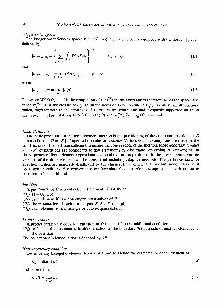
2.5.1. The Babuska and Rheinboldt estimator Consider piecewise linear approximation in one dimension. There are many types of a posteriori error

estimator available for this case. The purpose here is not to obtain new results, but to show how an existing estimator fits within the framework.

A superconvergence result is known for this situation (cf. [63]): if u E H3(0) and the mesh is quasi- uniform then

Iux - n 4 P H’(R) G a2 I4f’(R) (2.59)

where np interpolates at the endpoints of the elements. The recovery operator is constructed using the process shown in Fig. 1. The operator is linear and based on values of the direct approximation to the

gradient sampled on the set I? as shown in Fig. 1. It is easily verified that for any piecewise quadratic function u one has Gx(Qu) E u’. Moreover,

IwG_(K) G 3 14wI,x(K”). (2.60)

Therefore, (SC) and (Rl)-(R3) are valid. The estimator on element K is

77K = lIGx(ux) - 4AlL2(K)~ (2.61)

The estimator is precisely the estimator originally proposed and analyzed by Babuska and Rheinboldt [12](Definition 6.3). Previously, the estimator was obtained by an argument based on locally projecting the error onto a quadratic function that vanishes at the nodes. For further details see [12] where numerical examples illustrating the effectiveness of this estimator will also be found.

M Amsworth, J.T Oden/Comput. Methods Appl. Mech. Engrg. 142 (1997) l-88 17

m . . V- I? (a) Finite element approximation u

(c) Recovered gradient G{u).

Fig. 1. Construction of recovery operator GX = G from piecewise linear approximation in one dimension.

2.5.2. An estimator for quadratic approximation Consider approximation using piecewise quadratic functions in one dimension. The superconvergence

property holds in this situation (see [44]). A recovery operator Gx may be defined by exploiting the result: if the true solution is cubic then the true gradient U’ and the gradient of the quadratic interpolant fl,u, coincide at the nodes used in the 2-point Gauss-Legendre quadrature rule on the element. Therefore, on the element [xl, x,+~] we sample the gradient at the points

x+ = - 1 ; {

x, + &+I f -!- (Xl,, - XL> . d3 I

(2.62)

The next step is to define the recovery operator Gx. This is done by first recovering the gradient at the nodes and the centroid of each element. There are many possible ways to carry out this process (many of which fall within the framework). We shall use a cubic interpolation process to interpolate the gradient sampled at the Gauss-Legendre points. A procedure based on quadratic interpolation would meet the recovery criteria (Rl)-(R3) but would give an unsymmetrical scheme.

The recovery operator GX is as follows: l the value of GX[u] at the centroid of element [x,, x~+~] is taken to be the value of the of the cubic

polynomial interpolating to u’ at the points

ix:_1 > -y-J 4 > x,1 ) (2.63)

l the value GX[u] at a node X, is the value of the cubic interpolating to u’ at the points

{X,:&-+X7 (2.64)

l the function Gx[u] is taken to be the X-interpolant of the recovered values at the centroids and nodes.

It is easily verified using elementary manipulations that conditions (Rl)-(R3) are satisfied. Theorem 2.6 then shows the estimator is asymptotically exact. One could obtain an explicit expression for the estimator in terms of the values of the finite element approximation at the Gauss-Legendre points. However, this is unnecessary since the recovery process combined with a quadrature rule provides a simple method of implementation. Examples showing the performance of the estimator will be found in

PI.

18 M. Amworth, LT. Oden/Comnput. Methods Appl. Mech. Engrg. 142 (1997) 1-88

2.53. The Kelly, Gage, Zienkiewicz and Babuska estimator Consider the finite element approximation of Poisson’s equations using piecewise bilinear approxima-

tion in two dimensions. For the sake of simplicity assume each of the elements I( is a square with sides of length h parallel to the axes.

Results from Zlamal [63,64] show that the superconvergence property (SC) holds for this situation

IUX - Q&L(~) 6 Ch’ I&(n) (2.65)

where I$ is the bilinear interpolant at the vertices of the mesh. The recovery operator Gx is piecewise bilinear in each component. The values at the vertex x are obtained by a simple averaging of the gradient sampled at the centroids of the elements having a vertex at x (see Fig. 2). If (x,y) is a boundary vertex, then G,&](x, y) is the value at (x, y) of the bilinear function which interpolates to Vu at the centroids of the elements that are nearest to the point (x,y). The operator GX is linear and bounded since

IGx[41,x~,~ G 4 blw,.,,~~~ v’u E X (2.66)

and a straightforward manipulation reveals

GX[Z$v] - Vu (2.67)

whenever v is piecewise biquadratic. Consequently, the recovery operator satisfies conditions (Rl)-(R3) and (SC). The estimator Q on element K is

77~ = IlGx(ux) - V~XIIL~~K~~ (2.68)

This estimator will be asymptotically exact thanks to Theorem 2.6.

(a) Scheme for new estimator.

(b) Scheme for Kelly et al. estimator.

Fig. 2. Construction of recovered gradient at vertex of element K. The value at . is a linear combination of the values at o usrng

the weights indicated.

M. Aimworth, J.7: Oden/Comput. Methods Appl. Mech Engrg. 142 (1997) l-88 19

It is interesting to compare the new estimator with the estimator +jK proposed by Kelly et al. [40]:

and where

(2.69)

(2.70)

is the discontinuity in the finite element approximation to the gradient across the edge between neighbouring elements K and J. Using the midpoint rule for integration along each side of the element, the estimator (2.69) may be rewritten as

2

(2.71)

where the discontinuities are evaluated at the midpoints of the sides. Zienkiewicz et al. [59] state that the derivation of (2.71) is complex and subject to many heuristic arguments.

Kelly et al. [40] note that the estimator bears out practical experience that the accuracy of the approximation is related to the discontinuity of the finite element approximation to the gradient on the interelement boundaries. The recovery based estimator (2.68), like (2.71), is found after a lengthy but otherwise straightforward manipulation, to depend on the discontinuities in the finite element approximation to the gradient. The dependence is more intricate than in (2.71) involving, in addition, differences in tangential components at the centroids. The estimator (2.69) uses gradients sampled from the element K and elements sharing a common edge, while the estimator (2.71) also involves elements sharing a common node as shown in Fig. 2.

The estimator (2.68) may be simplified by avoiding terms arising from elements sharing only a common node. This may be achieved by taking the values of the recovered gradient at the vertices to be (see Fig.

2)

Gxbl(x,Y) = ; Ph/2h,y+1/2h + W+l/2h,y-1/2/J. (2.72)

The new recovery operator satisfies (Rl)-(R3) and gives rise to an estimator identical to $K. The estimator derived by Kelly et al. therefore may be viewed using the above framework. This approach makes the derivation of (2.71) straightforward.

It might seem that the estimator nK is too complicated to be of practical use. However, it is in many ways much simpler than the Kelly estimator. For instance, with the Kelly estimator it is not obvious how one should define the value of the jump along the exterior boundary 80. This difficulty does not arise with the recovery based estimator. The recovery based approach even provides the answer: the value of should be taken to be the jump on the opposite side of the element.

2.5.4. Zienkiewicz-Zhu patch recovery technique An alternative type of recovery estimator was introduced by Zienkiewicz and Zhu [61,62]. Let P

denote the set of vertices in the finite element partition. The recovery operator Gx is defined by first

identifying the patch fi, of elements having a vertex at X, E ?P. That is

?& = {K E P : K c supp em} (2.73)

where &, is the pyramid function associated with the node x,. An intermediate recovered gradient Gx,, is then constructed for each patch and the final recovered gradient is obtained by averaging

GxbxlW = & c Gx,mbxlW mttIr

(2.74)

The intermediate functions Gx,, are constructed using values of the gradient of the finite element

approximation sampled on the patch 6,. Let Z(m) denote the set of points at which the gradient is

20 M. Aimworth, J.7: Oden/Comput. Methods Appl. Mech. Engrg. 142 (1997) l-88

to be sampled. For instance, working with quadrilateral elements one would use the Gauss-Legendre quadrature points (see Fig. 3). For triangular elements, the set Z(m) consists of the points shown in Fig. 3. Further examples will be found in [61,62].

The function Gx., is obtained by calculating a least-squares fit to the gradient sampled at the points Z(m). The function Gx,, is assumed to be of the form X x X where X is the finite element subspace. That is

(2.75)

where &n(x) form a basis for the finite element subspace X and a;, are constant vectors chosen to minimize the expression

c {Gx,m(z) - %(z)}~ (2.76)

Of course, in the summation (2.75), only degrees of freedom associated with elements in the patch & need be considered. This means that the actual value of the final recovered gradient Gx on an element K

will depend only on values sampled from the patch K of elements neighbouring K. Therefore, condition (R2) will be satisfied. Equally well, the recovery operator is linear and bounded so that condition (R3) is also valid. The superconvergence condition (SC) and condition (Rl) can be satisfied by selecting the sampling points Z(m) to consist of the points at which superconvergence occurs. If this is the case, then the estimator will be asymptotically exact according to Theorem 2.6. This is confirmed in numerical examples [61,62]. However, it is often the case in practical computations that the superconvergence property is not satisfied, or, the sampling points may be chosen differently. The estimator might be expected to degrade in such circumstances. In fact, it is found that the estimator is astonishingly robust,

continuing to perform satisfactorily even in quite extreme situations [15,16]. While Theorem 2.2 suggests that the estimators might tend to bound the error asymptotically, the estimators remains an open question.

2.6. Summary

the reason behind the robustness of

The error estimation techniques often used in the engineering community and sometimes referred to as averaging based error estimators have been considered. The development can be thought of as consisting of two main parts. Firstly, the derivation of Theorem 2.2. As a special case, this shows that (for h sufficiently small) the averaging based estimators should tend to overestimate the true error.

(a) Degree p=l (b) Degree p=l.

w Degree p-2 (a) Dew= ~‘2

Fig. 3. Sampling set Z(m) for patch recovery technique.

M. Aimworth. J.7: Oden/Comput. Methods Appl. Mech. Engrg. 142 (1997) I-88 21

It is only if one wishes to obtain two-sided estimates or asymptotic exactness that it then becomes necessary to make the additional and rather stringent assumption concerning the superconvergence property. Under this condition, it was shown that a class of estimators based on the use of recovery operators GX will be asymptotically exact. The recovery operators are closely related to the averaging based schemes and in some cases are identical. In this respect, the theory developed for the recovery operators GX and the associated error estimators can be regarded as providing some indication of the behaviour of the averaging based schemes and how they might be modified to enhance their performance.

3. Explicit a posteriori estimators

3.1. Introduction

Consider the model problem in Section 1.5. Suppose that the finite element approximation zlX has been computed. The basic issue in a posteriori error estimation is embodied in the question: how can the discretization error e be estimated? In order to provide an answer one may make use of

l the Galerkin approximation ux itself l the data f and g l equation characterizing the true error:

B(e, u) = B(u, u) - B(ux-,ZJ) = L(V) - B(LIX, u) Vu E V (3.1)

l the Galerkin orthogonality property:

B(e, ZJX) = 0 Vux E x. (3.2)

The following section illustrates how these may be used to derive a simple a posterior-i error estimate.

3.2. A simple a posteriori error estimate

The first step is to decompose Eq. (3.1) for the error into local contributions from each element:

B(e, u) = L(u) - B(L(x, u)

(3.3)

for all u E V. Integrating by parts over each element gives

B(e,u)= c {lruh+JKmr KtP N

Ruds-LK,rN$uds}

where r is the interior residual

r = f +Aux -cu,y in K

and R is the boundary residual

(3.4)

(3.5)

R=g-$ ondKnTN K

(3.6)

where nK is the unit outward normal vector to dK. Each of these quantities is well defined thanks to the smoothness of the data and the regularity of the approximation ux on each element. The contribution from the final term in (3.4) can be rewritten by observing that the (trace of the) function u is continuous along an edge shared by two elements giving

(3.7)

where the final summation is over all the inter-element edges y on the interior of the mesh. The quantity

22 M. Aimworth, J.T. Oden/Comput. Methods Appl. Mech. Engrg. 142 (1997) IGQ?

dux i-1 dn = ?zK . (VUX)K + n.l. (VUX)J (3.8)

defined on the edge y separating elements K and J represents the jump discontinuity in the approximation to the flux. The identity (3.8) can be written more compactly by extending the definition of the boundary residual to incorporate the jump discontinuity in the flux. Therefore, on interior edges the definition (3.6) is augmented by

so that (3.8) then becomes

B(e,v)[email protected]+ C /Rvds VVEV KtP K y&P y

(3.9)

(3.10)

where the final summation is over all the edges in the partition P. The orthogonality property (3.2) may now be used as follows. For given v E V, let n,v be the

interpolant to v from the subspace X as in Theorem 1.1. Thanks to (3.2) and the identity (3.10) there holds

O=CJ rLfxvti+ C J

R&v ds. KEP K y&P y

(3.11)

Combining this with identity (3.10) gives

B(e,v) = C J r(v - n,v)dx+ C JR(v+v)ds VVE v. (3.12)

KEP K ytap y

The identity (3.12) plays an important role, indirectly or directly, throughout a posteriori error analysis. It may be used to derive the a posteriori error estimate as follows. Applying the Cauchy-Schwarz Inequality gives

B(eJ ‘) G c ikh.2(K) lb - n~viit2(K) + c IIRh&) II’ - n~v~~~2(y)

KEF YEW

Let K denote the subdomain consisting of elements sharing a common edge with element K

K=int{UJEP:JnK#0}

(3.13)

(3.14)

It may then be shown [26] that there exist a constant C which is independent of v and hK such that

[IV - nXvIILZ(K) 6 ChK IvI~‘(K”j (3.15)

and

where hK is the diameter of the element the Cauchy-Schwarz Inequality leads to

(3.16)

K. Inserting these estimates in inequality (3.13) and applying

B(e, v) < C lvlH~(~) C h2K I(lllt2c~) + C hK lIRlI&y, . KEP ytaP

(3.17)

Finally, noting that IvI~,(~) 6 I I Iv 11 I and substituting e in place of v gives the a posteriori error estimate

lllell? G C 1

c h”K b%,,(K) + c hK IIRit2(,, (3.18)

KEP yeap I

where I )).III denotes the energy norm for the model problem (l(~((1~ = B(v, v). Apart from the constant C, all of the quantities on the right-hand can be computed explicitly from the data and the finite element

M. Ainsworth, J. 7: Oden/Comput. Methods Appl. Mech. Engrg 142 (1997) I-88

approximation. Typically, the terms on the right-hand side are regrouped as follows:

IIle1112 G C c {“: IIyll~:(K) + ; hK II&K)} KG

23

(3.19)

The purpose in doing so is that defining the local error indicator by TK on element K by

7; = h; Ilriiil(K) + ; hK IIRk (3.20)

allows one to identify contributions from each of the elements. It is then assumed that each of these quantities is a measure of the local discretization error over each element. In this way one can use qK as a basis for guiding local mesh refinements.

Error estimators of this form were originally derived by Babuska and Rheinboldt [14] in one dimension: Babuska and Miller [lo] for bilinear approximation in two dimensions; and Kelly et al. [40]. Estimators that may be computed explicitly from the solution and the data are often referred to as explicit estimators.

3.3. A simple error estimator in the Lz norm

The estimator derived above gives information about the error measured in the energy (or any equivalent) norm. The duality argument due to Aubin and Nitsche [2.5] plays an important role in the derivation of a priori error estimates in norms other than the energy like norms. It may also be used in the context of a posteriori error estimators.

To apply the technique consider the adjoint of the original model problem:

@F c v : B(u, a+) = (F,u) vu E v (3.21)

where F E L2(,R) is given data. It is assumed that this problem is regular in the sense that the solution QF has the extra regularity QF E H2(L?) n V and the solution operator from LZ(fl) to H’(R) is continuous

II @FIIHyR) 6 c IIFIIL(r2) (3.22)

The specific choice of data F equal to the error function e then gives

I141Zz,lL~ = We, @A. (3.23)

The residual equation (3.12) plays the same role as in the derivation of the energy norm estimator

B(e, QcZ) = c / r(Qe - IIx@~,) dx+ c J’ R(Q& - I7,@,J ds (3.24) KEP K y@P y

and, as before, the Cauchy-Schwarz Inequality gives

B(e, ‘) G z: Ib%,(K, II’ - ~~“l~,l(K) + c IIRIIL2(y, lb - h”IiL2(y) (3.25) KEP yG?P

Slightly different approximation theoretic results are required; there exists a constant C which is independent of u and hK such that [26]

11’ - =dL(K) G Ch:, I4Hz(KI, (3.26)

and

11’ - fl&,(i?K, < Chz’ IuI~~(~). (3.27)

Substituting these estimates and applying the Cauchy-Schwarz Inequality leads to

II4 21,1, c c I@&(R)

and so, with the aid of the

112

c hi llrlt2(K) + c 4 llN2(Y) (3.28) KEP ycaP

regularity assumption (after bounding I@J&?(~, in terms of llell,z(.r2,) there

24

follows

M. Aimworth, J.7: Oden/Comput. Methods Appl. Mech. Engrg. 142 (1997) I-118

(3 29)

A rearrangement of the terms on the right-hand side gives an estimator similar to the one derived before, apart from a higher-order scaling

KtP ’ b

THEOREM 3.1. Suppose that the domain error indicator

(3.30)

0 is convex and that TJJ = da. Let q,,(K) denote the local

(3.31)

where r and R are the interior and boundary residuals. Then there exists a constant C depending only on the shape regularity of the elements such that

(3.32)

KtP

PROOF It may be shown that the adjoint problem satisfies the regularity assumptions when the domain 0 is convex. The proof then follows immediately from the above steps. 0

3.4. Equivalence of estimator

The estimator implied by Eq. (3.19) p rovides an upper bound on the discretization error up to an unknown constant. If the estimator is to be used as the basis of an adaptive refinement algorithm, then it is desirable that it be an equivalent measure of the error. That is to say, there should be a constant C which does not depend on the solution U, the data f and g or the mesh parameter h, such that

(3.33)

Shouid such an estimate fail to be valid, one cannot expect that the resulting adaptive procedure will be effective.

The problem of obtaining two sided bounds for explicit estimators such as the one derived in Section 3.2 was addressed by Verftirth [57] who devised the following technique.

3.4.1. Bubble functions

Let i? denote a reference element. The interior bubble function 3 : k H IR is the lowest-order polyno-

mial which vanishes on the boundary &JK and is non-zero on the interior of K. An edge bubble function is the lowest order polynomial which vanishes on all but one edge and is non-zero on the interior.

Triangular elements In the case of triangular elements

K={(x^,y^):O<x^<l; O<y^<l-2). (3.34)

The functions il, x2 and x3 denote the barycentric (area) coordinates on k. The interior bubble function s is defined by

s = 27&&& (3.35)

and the first edge bubble function is

2 = 4&X3. (3.36)

M. Ainsworth, J.7: Oden/Comput. Methods Appl. Mech. Engrg. 142 (1997) 1-88 25

Quadrilateral elements In the case of quadrilateral elements

K={(x^,y^):-l<x^<l; -l<y^<l}.

The interior bubble function 5 is defined by

$ = (1 - _?)(l - y”)

and the first edge bubble functions is

(3.37)

(3.38)

j; = ; (1 - ?)(l - y^). (3.39)

LEMMA 3.2. Let P^ c H’ (I?) be a finite dimensional space of functions defined on the reference element.

Then there exists a constant c^ such that for all v^ E P^

(3.40)

(3.41)

where the constant c^ is independent of 6.

PROOE It is easily seen that the mappings

GH { &E}“2

both define norms on the finite dimensional space P^. The results then follow immediately from the fact that all norms on a finite dimensional space are equivalent. 0

Let K E P be any element and FK : K H K be an invertible mapping. The associated bubble functions on element K are then defined by

$K = s o F$; jyr =jjoF;? (3.42)

It is assumed that the partition P is non-degenerate. Therefore, there exists a positive number hK and constants Cr, C2 and C, such that the following properties hold for each of the local mappings FK:

IIJKII 6 C,k I&‘II < C&‘; C;‘hi 6 ldet JKI < Cjhi (3.43)

where JK is the Jacobian of the transformation FK. The set P is defined by

P={coF,-‘:v^tP^} (3.44)

where P^ is a finite dimensional subspace consisting functions of defined on i.

THEOREM 3.3. There exists a constant C such that for all v E P

and

c-’ I141L2(K) 6 II@JIILz(K) +hfc lWIH’(K) G c IW*(K)

(3.45)

(3.46)

where the constant C is independent of v and hK.

26 M. Ainsworth, J.?: Oden/Comput. Methods Appl. Mech. Engrg. 142 (1997) Id8

PROOE The result follows by mapping to the reference domain K, applying the previous lemma and a standard scaling argument. 0

LEMMA 3.4. Let 7 c L3k be an edge and j; the corresponding edge bubble function. Let P be a finite

dimensional space of functions defined on i;. Then there exists a constant c^ such that

(3.47)

Suppose that v^ E P is extended to K according to the rule

E^G‘(x^, r^) = 2(%, jqu^(x^>

there exists a constant c^ such that

IIX~~II ffI(K^) 6 c^ll~li,L(~)

In each case the constants c^ are independent of 6.

(3.48)

(3.49)

PROOF: The proof is based on the equivalence of norms on a finite dimensional space similar to before. •I

A scaling argument can be used to translate these results to a general element K.

THEOREM 3.5. Let y c dK be an edge and xy the corresponding edge bubble function. Let P be the

finite dimensional space of functions defined on y obtained by mapping P c H’(K). Then there exists a constant C such that

C-l llull:,(y, 6 .I

xvu* ds G C I141~Z~y, . (3.50) Y

Moreover, there exists an extension of v to K (again denoted by v) such that

h,“’ IIx&.,~~~ + h?* Ixv4w(~, 6 C II~IL,~~)

In each case the constants C are independent of u.

(3.51)

3.4.2. Bounds on the residuals The proof of equivalence makes use of the residual equation (3.10) in conjunction with special choices

of the function u. The first task is to bound the term Ilrllt,,cK,. Let TK be a polynomial approximation to the interior

residual r on element K. For instance, TK might be the L2(K) projection onto piecewise constants. Applying Theorem 3.3 gives

(3.52)

The function u = TKeK vanishes on the boundary of element K. It may therefore be extended to the whole of the domain 0 giving a function u belonging to the space V. The residual equation (3.10) then implies

B(e,%+K) = s

+KrrK d” K

where the first term contains contributions from element K only. Therefore

(3.53)

J GKF~&= J @KTK(?K -r)dX+B(e,rKcCII() (3.54) K K

M. Amsworth, J.7: Oden/Comput. Methods Appl. Mech. Engrg. 142 (1997) 1198 27

The first term on the right-hand side may be bounded as follows: by Cauchy-Schwarz

J kFK(YK - y)b G II~K6IIL(K) FK -k(K) K

and then by Theorem 3.3 (Part 2)

Il~K~KIIL2(K) G c IIW2(K)~ The second term is dealt with similarly

B(e,TKk) G lll4ll~ II~K~KII~~~~) and by Theorem 3.3 (Part 2)

llvk~k. IIHW G Chi’ IIrK IIL,K) . Therefore,

(3.55)

(3.56)

(3.57)

(3.58)

IIc&I(K) 6 C~~,‘IIl4IIK + IFK - ~llL(K,I (3.59)

and equally well, by the Triangle Inequality

llrll L(K) G w,‘IIlelIIK + IIFK - rllL(K,~~ (3.60)

It remains to bound the terms IIRIILZcY,. The argument proceeds in an analogous fashion. Let R, be a

polynomial approximation to the boundary residual or jumps. Theorem 3.5 gives

llw.,cy, G c J x3: ds. Y (3.61)

Let 7 denote the subdomain of R consisting of the union of the side y and the pair of elements (K and J say) sharing the common side y. The function u = R,xV vanishes on the boundary of the subdomain 7 and is continuous. Extending to the whole of the domain 0 gives a function u from the space V. The residual equation (3.10) with this choice of u yields

B(e,&xy) = _xrrR, d.~+ J J

xr RR, ds . Y Y

(3.62)

Therefore,

J xYi?: ds = _XqR, ds. Y .I

x&(& - R) ds + B(e,XyR,) - (3.63) Y .I Y

Each of these terms may be dealt with using Theorem 3.5 and the Cauchy-Schwarz Inequality as follows:

I XY~Y@Y - R)ds 6 ~~~y~yII~.,~y,Ilxy(~y - Rk,cy, 6 CII~,IIL~,)~~~~ - Rll~~(~) (3.64)

. Y

B(e3xy%) 6 Cll1411;Ilxy~yll~2~y) 6 C~~1’2111411;ll~yll~2~y) (3.65)

and

J _XY~RY ds G Il~ll~,~~~llxy~yII~~~r~ G ~~~ll~ll,~i;~II~yIlI-2~Y). (3.66)

This m:y be used to estimate llRl[ t,z(r) after using the Triangle Inequality and (3.60) giving

II%cy) G C{h,“2%ellty + hr1lG - rIILZ(K) + II& - R(lLZcV)>. (3.67)

LEMMA 3.6. Let r and R denote the interior and boundary residuals associated with the finite element approximation constructed from the subspace X. Suppose that TK and R, are finite dimensional approximations to the residuals on an element K and an edge y c dK. The approximations need not be globally continuous. Then there exists a constant C depending only on the shape regularity of the elements such that

lkll L2(K) 6 C~h~1111411~ + 11% - rllLz~K~~ (3.68)

and

28 M. Ainsworth, J.?: Oden/Comput. Methods Appl. Mech. Engrg. 142 (1997) I-88

IlRll Lz(r) G ~~~~1’2111elll; + hly/” 11% - 41L2cKj + II& - RIIL~(~)I. (3.69)

PROOF Follows from the previous arguments. 0

3.4.3. Proof of equivalence Lemma 3.6 is used to analyze the error estimator as follows. Choose the approximation rK to be

LZ(K)-projection of the residual r onto the degree p polynomials which are restrictions of elements of X to the element K. Similarly, the approximation RY is the L2(y)-projection of the boundary residual R onto degree p polynomials (this time in one variable) which are the restrictions of elements of X to the single edge y. Lemma 3.6 then applies giving

lb-II &(K) G w,‘IllelIlK + IIFK - ~IIL*(K,~ (3.70)

and

IIRII Lz(r) 6 C~~~‘/2111elll-; + hy* II% - rIlL2(K) + II% - RIIL&. (3.71)

For interior edges, the boundary residual R is simply the jump in the normal derivative which is itself a polynomial of degree p in one variable. Thus, one has RY E R on interior edges. Conversely,

on the exterior boundaries, one has R, - R = g - L$,g, where I&g is the polynomial approximation to g on the edge y, Noting that the data c for the original differential equation was constant leads to TK - r = f - I&f on each element K. Therefore,

IHI L&Y) 6 C~~,‘lll4IIK + Ilf - 4fllL,(KJ (3.72)

and

IIRII Lz(r) G W~1’zll1411~ + Q* Ilf - QflIL2(K) + Ilg - ~p&2(ynrN)I. (3.73)

The local error indicator vK in (3.20) associated with the element K can then be bounded by

77; 6 C 1

lll~lll~ + G Ilf - L&f II& + c hK II&T - 4&2(v) i

(3.74)

yC8Kfll-N

where the constant C depends only on the shape regularity of the element. The estimate shows that the error indicator is local in a certain sense, since the terms on the right-hand bound involve only contributions from the actual element and its immediate neighbours. Summarizing the results so far

THEOREM 3.7. Let VK denote the local error indicator

& = hi Iklt,(K) + ; hK IIRIt,(i3K, (3.75)


< c llkll12 + c hi Ilf - n,fIl;,~K, + c hK llg - LT~gll?,z(vj KEP KEP YCrN

Moreover, the local bound

& 6 C Ill4ll~+h~ Ilf - 1_I,fll;,(K, + c hK llg - LT~gll;l(vj yctJKrT~

is valid.

1. (3.76)

(3.77)

PROOF Follows from previous arguments. 0

M. Ainsworth, J.T Oden/Comput. Methods Appl. Mech. Engrg. 142 (1997) l-88 29

Typically, the terms involving the differences f - ZZPf and g - Z&g will be small compared to the other terms. In this sense, the estimator obtained by summing the local indicators provides an equivalent measure of the actual error in the energy norm. The local bound (3.77) is of importance for the design of adaptive algorithms showing that the estimator gives some indication of the error distribution and not simply a global bound.

3.5. The effect of numerical quadrature

In practice, the error indicator rlK will not be computed exactly since the integrals of the residuals will be performed using numerical quadrature. That is to say, the actual error indicator qK will be given by

(3.78)

where TK and &, are once again finite dimensional approximations of the actual data (but not necessarily the same choices as previously). In fact, if the data is continuous then the numerical quadrature would correspond to taking TK to be the polynomial ZPr which interpolates the residual r at the quadrature

points. Equally well, the approximation R, would be the polynomial Z,R (this time in one variable) which interpolates to R at the quadrature points on the boundary. This estimator can be analyzed as follows. Firstly, applying the Triangle Inequality gives

(3.79)

With the aid of Lemma 3.6 and proceeding much the same as before one obtains

Combining these results gives a result derived by Verftirth [56] (but see also [lo] and Section 4.2.4):

THEOREM 3.8. Let q~ denote the local error indicator

(3.81)



(3.82)

(3.83)

is valid. If the data f and g is smooth then the extra terms appearing in the bounds can be neglected showing that the estimator is in this sense equivalent to the actual error.

3.4. Error estimators for W,‘(n) and LP(0)

3.61. Estimates in W,‘(n), 1 < p < cc The basic argument used to derive the simple error estimator in the energy norm can be

to obtain estimates in the norm on the space W,‘(n). Let q denote the conjugate exponent generalized

30 M. Ainsworth, J.7: Oden/Comput. Methods Appl. Mech. Engrg. 142 (1997) 1-88

l+L1 54.

The residual equation (3.12) gives (with nX as in Theorem 1.1)

(3.84)

IWv4I = C / 0 - IIxu)dx+ c / R(u - &u)ds KG’ K y&v y

and applying Hiilder’s Inequality gives

(3.85)

IB(e~U>I 6 c biIL,(K) 11’ - H&(K) + c IIRIiL,(y) 11’ - nx”ll&(,) ’ (3.86)

KEP YEW

Slightly different approximation theoretic results are needed; there exists a constant C which is independent of u and hK such that [26]

IIu - nX"llLq(K) 6 ChK lUIw@) Y

and

lb - n~"IIL,(~K) ’ < Ch;-“’ lul,,, .

Substituting these estimates and applying Hijlder’s Inequality leads to

IB(e,U)l G c k&;(n) c h”K Ib-II:p(KJ + c hK lI%,p(Vj

1 KEP Y@p 1

I/P

.

As usual, the terms may be rearranged to identify contributions from each element

THEOREM 3.9. Let VW;(K) denote the local error indicator

v;;(K) = h$ Ilrl$,(K) + ; hK IIRIIP,,(%) (3.91)


(3.87)

(3.88)

(3.89)

(3.90)

.

PROOF: The result follows on observing that

((e((,;(,) 6 C sup B(e’u) UEWJ(L!) IIUllw:v4

(3.92)

(3.93)

and then using the above arguments. q

The effects of using numerical quadrature to approximate the integrals in the estimator can easily be incorporated.

3.6.2. Estimates in Lp(0), 1 < p < 00 One might suspect that the same basic argument used to obtain estimates for the error in the Lz norm

can be extended to the L, case. Once again, the Aubin-Nitsche Trick [25] is the essential idea. Consider the adjoint of the original model problem:

@FEV:B(u,@F)=(F,u) VUEV (3.94)

where F E Lq(0) is given data. It is assumed that this problem is regular in the sense that the solution @F

M. Ainsworfh, J.7: Oden/Comput. Methods Appl. Mech. Engrg. 142 (1997) I-88 31

has the extra regularity GF E lV~(0) n V and the solution operator from &(a) to IV:(n) is continuous

lI@iFllW;(“, 6 C lIFlIL,(n, . (3.95)

The specific choice of u equal to the error function e then gives

(e, F) = B(e, @F). (3.96)

The residual equation (3.12) is used as before.

(3.97)

and applying Holder’s Inequality gives

B(e,F) < c bib,,(K) lb - nx”b,q(K) + c IiRii~,(y) 11’ - n@lk,~y) . (3.98)

KtP YE*

The appropriate approximation theoretic results are that there exists a constant C which is independent of u and hK such that [26]

]I” - nX”lb,,(K, G Ch2, Iulw:(~) (3.99) 4

and

11’ - @&,(OK) --. < Ch;“’ II&,;,, .

With the aid of Holder’s Inequality

i

IlP

(e, Fl < C I%lqp, C @’ II’llpLp(K) + C hp IIRII&U) KEP YE@

and, thanks to the elliptic regularity assumption there follows:

Cc FJ G C IIFIIL,cn) C f$’ II’IIpLp(K) + C h? IIRII~p~,) . KcP YE*

A rearrangement gives an estimator in the familiar form apart from a different scaling

(e, F) 6 c IIFIIL,(,) hz iI’(I;JK) + ; hp IIRIIP,J~fQ ’

(3.100)

(3.101)

(3.102)

(3.103)

THEOREM 3.10. Suppose that the domain fl is convex. Let q&(K) denote the local error indicator

7);,(K) = h? IIrII;p(K) + ; hF IIRIIP,p(aK) (3.104)


llP

llell LJQ) ’ (3.105)

PROOE The adjoint problem satisfies the regularity assumptions when the domain 0 is convex. The proof follows using the identity

lkll k F)

Lp(f2) = F:& IIFIILq(,) (3.106)

and the previous arguments. •I

32 M. Ainsworth, J.7: Oden/Comput. Methods Appl. Mech. Engrg. 142 (1997) IL88

4. Implicit a posteriori estimators

4.1. Zntroduction

Sections 2 and 3 deal with estimators that can be computed directly from the finite element approximation and the data for the original problem. The methods described in the present section require the solution of a local boundary value problem approximating the residual equation satisfied by the error itself. The local error estimator is the norm of the solution of the problem. Such schemes give rise to implicit error estimators. The boundary value problems are local in the sense that they are posed either over a single element or a small subdomain of elements.

One might wonder whether it is worthwhile considering implicit estimators at all, since explicit schemes are apparently much simpler. There are good reasons for using implicit schemes. Firstly, the explicit estimators lead to local error indicators containing generic constants. These constants are, in general, unknown. In practice, one can try to find a suitable bounds on the values of the constants. However, the values of constants would be dictated by the worst case scenario and therefore would usually give pessimistic estimators. Secondly, there are two types of residual present in the explicit estimators corresponding the interior and the boundary. The correct relative weighting to attach to each type of residual is far from obvious. In addition, it is conceivable that there are cancellations between the two types of residual that is lost when one deals with each separately.

Implicit estimators, and the element residual method in particular, avoid such issues by solving a boundary value problem with the residuals as data. In this way the generic constants are avoided and the correct balance between the two types of residual is catered for by the solution process itself. The drawback is that one is obliged to solve an auxiliary problem requiring an appropriate approximation scheme; as we shall see, this creates its own difficulties.

The ideas will be illustrated by considering the model problem in Section 1.5. The basic idea is to approximate the residual problem characterizing the true error:

B(e, u) = B(u, u) - B( Ux,U) = L(u) - B(ux,u) Vu E v. (4.1)

4.2. The subdomain residual method

A method for a posteriori error estimation based on solving local residual problems with homogeneous essential boundary data over small patches or subdomains of the domain 0 was devised by Babuska and Rheinboldt [13]. The approach is particularly noteworthy because it provides a generally applicable method of a posteriori error estimation with firm theoretical foundations. Here, it will be assumed that the partition ‘P is locally quasi-uniform, although Babuska and Rheinboldt [13] dealt with more general classes of partitions (see also [lo]).

4.2.1. Formulation of subdomain residual problem Let IP denote the set of element vertices in the partition P and { &}nCP denote the first-order Lagrange

basis functions based at the element vertices. These functions are characterized by the conditions

6&&Z) = &Z, (4.2)

where x, is any vertex in !P and

c e,(x) - 1, x E n. (4.3)

The support & of the nodal function 0, consists of the patch of elements containing the vertex x,. The method is formulated starting with Eq. (4.1) characterizing the true error e E V. The usual consid-

erations apply: while, in principle, one could approximate the solution of this equation using a refinement of the finite element subspace X, it would be simpler to compute a new finite element approximation directly. The underlying idea is to replace the single global problem characterizing the error by a sequence of independent problems posed on small subdomains of the partition P. The nodal basis functions may be utilized for this purpose. With the aid of property (4.3)

M. Ainsworth, J.?: Oden/Comput. Methods Appl. Mech. Engrg. 142 (1997) I-88 33

(4.4)

where u E V. Each of the functions &u belongs to the space Hi(fin). Define the local bilinear form

B, : HA(&) x H;(ti,,) I--+ lR by

&(K u) = J

2 (Vu.V u+cuu) dx n

and the local load functional L, : Hi(k) ++ IR by

(4.6)

The subdomain residual problem is to find & E HA(k) such that

B,(&, u) = L,z(u) - B,(ux, U) ‘du E H;(h). (4.7)

Motivated by Eq. (4.4), the error estimator nn associated with the subdomain fi, is taken to be

%I = Ill+~lll~~ (43)

and the global error estimator TI is obtained by summing

1 1

112

77= En; . (4.9) nt’Y

In practice, the subdomain residual problems are approximated using a finite dimensional subspace of

Hi(&). We shall return to this point in Section 4.2.4.

4.2.2. Nomenclature and assumptions Suppose that the basis function 0, is non-zero on an element K; then

and, that

lhz(4l 6 1, XEK (4.10)

moreover, there exists a constant C depending only on the non-degeneracy of the element such

It is

IV&(x)l f C/z,‘, x E K. (4.11)

possible to partition the set of vertices W into the union of disjoint subsets F1, ?P2,. . . such that any pair of nodal basis functions in the same subset !PF have non-overlapping supports. Specifically, the condition that will be required is

VO,, 0, E !Pr : m # n * suppO& rl supp”f3, is empty (4.12)

where supp’8, denotes the interior of the support of 0,. It is easy to see that this process is always possible since one can simply choose each of the sets ?Pr to consist of a single basis function. Later, it will be found advantageous if this is accomplished using as few subsets as possible. The smallest number of subsets will be denoted by p and referred to as the overlap index for the partition.

Let K be any element in the partition P. The set of basis functions which are non-zero on this element is denoted by c+(K). The maximum cardinality of any of these sets is denoted by T and referred to as the intersection index. If the partition is locally quasi-uniform then the intersection index will be equal to the maximum number of vertices in any element. However, if the mesh is not proper then the intersection index may increase without bound as the refinement progresses. Such a situation is disallowed by requiring the intersection index 7 and the overlap index p are uniformly bounded for the family of partitions.


The subdomain consisting of the elements which neighbour element K is denoted by

K = int {

U7 : I n 72 is non-empty} . (4.13)

Since the elements are non-degenerate the maximum number of elements contained in any of these subdomains is bounded by a multiple of T. Local approximation properties will be needed. In particular, there exists [26] a constant C such that for any u E H’(0) and any element K there holds

hK1 Ilu - Q@lIL2(K) + lu - n&*(K) 6 C IuIH’(;, (4.14)

where ZI, is as in Theorem 1.1. The assumptions are true regardless of the polynomial degree actually used to construct the finite ele-

ment subspace, and merely impose restrictions on the mesh topology and mesh geometry. The conditions are always satisfied should the partition be locally quasi-uniform.

4.2.3. Equivalence of estimator LEMMA 4.1. Suppose that the above conditions hold. Then there exists a constant C depending only on the non-degeneracy of the elements such that for any u E H’(0)

c IlM~ - mN&‘) 6 CT2 Ikl;yn,f (4.15)

ntlY

PROOE Let K be any element and 0, E YP be a nodal basis function which does not vanish on K. Then,

Il&(u - rr,~)ll& 6 lle,ll;&, lu - rrx4zHl(K) + lBnl2w~~(K, lb - ~&K~~ Thanks to properties (4.10)-(4.11)

2 II @z(u - b4Ilfp(K) 6 C{lu - &4&~) + hi2 Ilu - h4t2(~~~

and using the approximation property gives

Ilel(~ - @Y~M&K, 6 c l&E). Summing this inequality over all vertices gives the result

THEOREM 4.2. Let v,, denote the local error estimator obtained using the subdomain residual method. Then there exists a constant C depending only on the non-degeneracy of the elements such that

rl < lllelll 6 C~71 dz

(4.16)

where r is the overlap index and p is the intersection index.

PROOR Using the Galerkin orthogonality

B(e, u) = B(e, u - Ilxu)

and then by property (4.3)

M. Amsworth, J.7: Oden/Cotnput. Methods Appl. Mech. Engrg. 142 (1997) l-88

B(e, u) = C B(e, Mu - Hx~)) IlEP

and noting that 6,(u - nxu) E HA(&)

B(e, u) = c B($n, Mu - flxu)). NT

Hence

IB(e,u)l 6 C rlJll%(u - fl~u)lll. nt’Y

Applying the Cauchy-Schwarz Inequality and Lemma 4.1

from which the result follows immediately

lll4ll G CT Conversely, consider

G lllelll IllC 44 IlEP

By partitioning the set F of vertices as described above

IIIC 411112 = IIIC c 4nll12 6 PC IIIC ~nll12 = PC c lll~nll12 nt’Y T, ncly, % ncly; y: ntly,

where property (4.12) has been used. Consequently,

IIIC 4Jnll12 G PI* ntF

and the result follows immediately. 0

4.2.4. Treatment of residual problems The subdomain residual method described above requires the exact solution of the local problems

6, E H;@%) : &(4n,un) = L(urz> - &(~x,un) VJV, E H,#n>. (4.17)

In practice, the method is seldom used, partly because it is inconvenient and relatively expensive to

develop approximations over the patches ?&. Babuska and Miller [lo] circumvented this difficulty by obtaining an equivalent measure for the local error estimator ) ( I& I I I as o f 11 ows. Integrating the right-hand side of (4.17) by parts gives

L(u,) - B,JU~,U,J = c

KG%

(4.18)

36 M. A&worth, J.Z Oden/Comput. Methods Appl. Mech. Engrg. 142 (1997) l-88

where r and R are the usual interior and boundary residuals. A routine application of the Cauchy- Schwarz Inequality leads to the bound

77n 6 C

i

iI2

c h; 1(‘1/& + c hK llK&,) . (4.19)

KG” VCR, 1 Summing this estimate over all vertices in the partition and regrouping the terms leads to the familiar explicit error estimator

lll4ll 6 cc 4 (4.20) KEP

where

n; = ii’/i;~(K) + c hK IIRit+). (4.21)

Babuska and

c hK

KG”

where

ycaK

Miller also obtain the following result:

lb-II Lz(K) + c h? IIRIIL,~~~~ 6 c(‘h + E) YCQI

(4.22)

E = c hi ll’lltZ(K) + c hrl/R - %llq+ (4.23)

K& YCn,

This result is essentially identical to those derived in Section 3.4 when considering explicit error estimators but predates the discovery of those estimates.

4.3. The element residual method

4.3.1. Formulation of local residual problem In principle, one could approximate the problem (4.1) and obtain an approximation to the actual

error function. The optimality of the Galerkin method and the associated orthogonality property of the error, means that one must use a larger subspace than the original finite element subspace X if one is to obtain a non-zero approximation to the error. The cost of solving the problem would be comparable with simply resolving the original problem using the finer discretization. One can attempt to reduce the cost of solving this global problem by replacing it by a number of independent local problems posed over each element in the domain. The local problems could then be approximated relatively inexpensively and even solved in parallel.

Let the error on an element K be denoted by e = u - UX. Thanks to the smoothness of the finite element approximation on the element interiors, one finds that the error satisfies the differential equation

-Ae+ce=f+Aux-cux inK. (4.24)

The major difficulty is to supplement the equation with appropriate boundary conditions. There are various cases to consider. First, suppose that the element K intersects a portion of the boundary of the domain 0 where an essential boundary condition is imposed. The appropriate boundary condition for the local error residual problem is clearly

e=O ondKnro. (4.25)

Here, it has been assumed that the finite element approximation has been constructed so that the essential boundary conditions are satisfied exactly (although this is not essential). Next, suppose that the element intersects a portion of the boundary dR where a natural boundary condition is imposed. The local error residual problem is subjected to a natural boundary condition

de dUX - ondKnTN.

G =g- &K (4.26)

M. Amsworth, J.T. OdenlComput. Methods Appl. Mech. Engrg. 142 (1997) 148 37

So far, appropriate boundary conditions have been clear. It remains to consider the case when the element boundary lies on the interior of the domain. The first decision is whether to impose an essential or a natural boundary condition. The element residual method is based on using a natural boundary condition. Ideally, one would like to impose the condition

de du 8uX -=--- f%rK d/Q an, K

(4.27)

on the edge separating elements K and 1, where uXIK denotes the restriction of the finite element approximation to an element K. Unfortunately, the true flux appearing on the right-hand side is unknown in general. However, one may replace the true flux by an approximation obtained from the finite element approximation itself

(4.28)

where we define

-= ; nK ’ {(vu,), + (vux)J) ’ (4.29)

The motivation for this choice is founded on the hope that by averaging the discontinuous finite element approximation to the normal flux one obtains a reasonable approximation to the true flux.

The error residual problem is formulated as a variational equation as follows. On each element K the actual error satisfies the boundary value problem

BK(e,v) = FK(v) - BK(ttX,v) + J au - vds \Ju E VK. aK anK

(4.30)

Here,

VK = {V E H’(K): u=OondKnTD} (4.31)

and B K : VK x VK H ]R is the local bilinear form

BK(u, v)= s

(VU. VU+ CUV) du (4.32) K

and FK : VK H R is the local load functional

FK(v) = KfvdY' .I (4.33)

The error residual problem is the weak form of the problem specified by the conditions (4.24)-(4.28): find & E VK such that

BK(+K,V) =FK(V)--~(Ux,v)+ J,,(z)

vds VuEVK. (4.34)

Here, the definition of the average has been extended to include the portion r~ of the exterior boundary

(4.35)

The question naturally arises as to whether there exists solutions of the residual problem (4.34). In general, the answer is negative! The difficulty arises from the non-trivial kernel of associated with the bilinear form BK(., .). Unless the data satisfies appropriate compatibility conditions, the problem will fail to possess solutions. Therefore, extra assumptions must be made to ensure well-posedness. One alternative is to work on a subspace of VK on which the bilinear form will be coercive. This approach, although apparently crude, leads to useful error estimators. An alternative approach is to try to choose the boundary data more carefully so that the underlying problem is naturally well-posed so that there is no need to resort to altering the space V K. This approach, known as the equilibrated residual method, will be discussed in the next section.

38 M. Ainsworth, J.?: Oden/Comput. Methods Appl. Mech. Engrg. 142 (1997) 138

4.3.2. Subspaces for the element residual method The error residual problem (4.34) is an infinite dimensional problem. The element residual method

is obtained by constructing particular finite dimensional subspaces YK of the local spaces V,. Here, the discussion is restricted to first-order finite element approximation; the general case will be dealt with later.

Quadrilateral elements Consider the case of finite element approximation using piecewise bilinear functions on quadrilateral

elements. The local approximation space for the error residual problem is constructed using the basis functions specified on the reference element

K={(x^,y^):-l<x^<l; -l<F<l}. (4.36)

The edge bubble functions are given by

(4.37)

j;, = ; (1 - P)(l +y^>

24 = ; (1 - y^2)(1 - x^)

and the interior bubble function 6 is given by

$ = (1 - P)(l -r”). (4.38)

The space Y is defined by

Y = span{?i7%,G,&, S> (4.39)

and the error residual problem is approximated using the subspace YK obtained by mapping the bubble

space r to the element K.

Triangular elements The paper by Bank and Weiser [23] on the element residual method considered the case of finite

element approximation using piecewise affine functions on linear triangular elements. The local approximation space for the error residual problem is constructed using the basis functions specified on the reference element

K={(x^,y^):O<x^<l; O<y^<l-2). (4.40)

The functions x1, x2 and x3 denote the barycentric (area) coordinates on i and the edge bubble functions are given by

2, = 4X&; j;, = 4X,&; 2s = 4&x2. (4.41)

Let Y denote the space

Y =van{%,?2,5?33). (4.42)

The error residual problem is approximated using the subspace YK obtained by mapping the bubble

space Y to the element K. The bubble space suggested by Bank and Weiser contains no interior bubble function. Verftirth [56] has suggested an alternative bubble space based on including the extra interior bubble function.

In each of these cases, the basic pattern for approximating the local problem (4.34) is to increase the order of the space used to construct the original finite element approximation and then factor out the

M Ainsworth, J.7: Oden/Comput. Methods Appl. Mech. Engrg. 142 (1997) I-88 39

functions which are non-zero at the vertices of the element. This may be achieved by subtracting the interpolant in the original finite element space.

The discussion has been restricted to first order finite element approximation. For higher-order approximation, some care has to be exercised when selecting the subspaces with which to approximate the residual problem (see [3] and Section 4.5.3).

4.3.3. The classical element residual method The classical error residual method [22,23,29,48] for a posteriori error estimation is to solve the local

error residual problems

thereby obtaining a function &. The local error estimator qK on element K is defined by

77K = lll+KlllK

and the global error estimator is obtained by summing the local contributions

As remarked earlier, such estimators will be referred to as implicit estimators.

(4.43)

(4.44)

(4.45)

4.4. Equivalence of estimator

4.4.1. Relationship with explicit error estimators The implicit estimators can be related to the explicit estimators of Section 3. By applying Greens

identity to the right-hand side of the error residual equation (4.43) one obtains

B~(+K,v)=~rvdx+~KRvds VVE YK (4.46)

where r and R are the precisely the interior and boundary residuals appearing in the explicit error estimators. Choosing the function u to be the estimated error function & leads to

(4.47)

The function & belongs to a finite dimensional space. Moreover, if the gradient of & vanishes then & itself must be the zero function. Therefore, there exists a constant C which depends only on the shape regularity of the element K but not on its size such that

II& IL(K) 6 ChK I$KIHI(K) (4.48)

and for any edge y c dK

II+KIIL(~, G ch~2 khIH'(K) . (4.49)

With the aid of these results and the Cauchy-Schwarz Inequality

7; G C hi IlrllL,c~, + C h:* IIRIIL2cY~ 1

I~‘KIw(K) (4.50) yc3K

from which one can deduce that

“rlK G c hi I&K, + ; c hK IIRit,(y, ycaK

(4.51)

where term on the right-hand side is the explicit error estimator discussed earlier.

40 M. A&worth, J.T OdenlComput. Methods Appl. Mech. Engrg. 142 (1997) l-88

4.4.2. Further bounds Suppose that the space YK used to approximate the error residual problem is equipped with an interior

bubble function. This assumption rules out the space chosen by Bank and Weiser [23] for piecewise affine approximation on linear triangles, but is satisfied if the space is chosen as suggested by Verfurth [56]. Let +K E YK denote the interior bubble constructed in Theorem 3.3. The following result complements Lemma 3.6:

LEMMA 4.3. Let r and R denote the interior and boundary residuals associated with the finite element approximation constructed from the subspace X. Suppose that TK and R, are finite dimensional approximations to the residuals on an element K and on an edge y c 8K, and let 77~ denote the element residual error estimator Then there exists a constant C depending only on the shape regularity of the elements such that

llrll L,(K) 6 C{h,‘qK + tirK - ‘iiL2(K)) (4.52)

and

IlRll Lo G C{h,“‘W +hr iirK - ‘th&K) + 11% - RIkzcr,b (4.53)

PROOF The first result is shown by following the arguments from (3.52) to (3.60), except that the identity (obtained by choosing u = T;K$K in (4.43))

BK(+KyFK$K) = k +KrrK dX

is used in place of (3.53). The second result is obtained by following similar arguments to those from (3.61) to (3.67) and using the identity (which follows from (4.43) with the choice u = RYxY)

BKb#‘K,&Xy) = J

rR,XV dx + J

xr RR, ds K Y

instead of (3.62). 0

4.4.3. Proof of equivalence Thanks to the relationship between the explicit and implicit error estimators, one immediately obtains

the following result as a corollary of Theorem 3.7 (cf. [56]):

THEOREM 4.4. Let 77~ denote the local error estimator obtained using the element residual method. Then there exists a constant C depending only on the shape regularity of the elements such that


77; 6 c {

I II4 115 + hi Ilf - n,f &K, + c hK k - &&,(yj

yCOKflr~

(4.55)

holds for all elements K E P. As noted elsewhere, the extra terms depend on the smoothness of the data and will often be negligible in comparison with the estimator and the actual error. In this sense, the element residual method gives an equivalent measure of the discretization error in the energy norm.

4.4.4. The effect of numerical quadrature In practice, just as for explicit error estimators, the computations of the the integrals appearing in

the element residual equation will be performed using numerical quadrature. Therefore, the computed

M. Ainsworth. J T Oden/Comput. Methods Appl. Mech. Engrg. 142 (1997) I-88 41

error estimator jjK will be obtained by solving the perturbed problem

?K E YK : BKGK,U) = ZKW - BK(UX,U) + s,, (2) vds VvgYK

and where EK : YK H IR is the functional

(4.56)

(4.57)

where ZPf and Z,g are the polynomials which interpolate to the data at the quadrature points (assuming the data is sufficiently smooth). This estimator can be analyzed by noting that

BK(~KIU) = BK(+‘K,U) + J’

K(f-4f)U~+ s

(g - 4&u ds aKnr N

from which one obtains

(4.58)

(4.59)

This estimate used in conjunction with the previous result gives:

THEOREM 4.5. Let ijK denote the error estimator obtained from the element residual method in the presence of numerical quadrature. Then there exists a constant C depending only on the shape regularity of the elements such that

lliell12 < c c 5; + c hi llf - Ipf lt2(K) + c hK llg - zP&,2(y)

KcP KtP WTN


is valid.

Illelll$+h~ ltf -z/Jfll;2(K) + 1 hK llg-zd,zc,)

ycaKnr~

(4.60)

(4.61)

4.5. Performance of estimators

The robustness and quality of estimators along with the identification of limits of their performance is of vital importance. Studies of this type have been undertaken by Babuska et al. [15,16]. Here, the influence of the subspace used to solve the element residual problem is studied. In practice, the only feasible approach is to construct an approximate solution to the local problem. The choice of subspace used for first-order finite elements is reasonably well established and understood: see for example [23] and Section 4.3.1. For higher-order finite element approximation, the situation is less clear and some unpleasant surprises are lurking.

Although the classical element residual method is popular, relatively little is known about its performance. For instance, it was only comparatively recently proved by Duran and Rodriguez [31] that the classical element residual error estimator converges to the actual error in the energy norm for regular solutions on parallel meshes of linear triangular elements.

Throughout, it will be assumed that the mesh and the true solution are as regular as necessary for the analysis. This is an unrealistic assumption from the practical viewpoint, but serves to isolate the effects associated with the approximate solution of the local residual problem from effects due to singularities, non-smooth domain, irregular meshes and so on. A simple test of the performance of an error estimator is consistency (or asymptotic exactness). Roughly speaking, an a posteriori error estimator is said to be asymptotically exact if the ratio of the estimated error to the actual error tends to unity as the mesh size tends to zero. Whilst asymptotic exactness should not be over-emphasized, it is useful to understand


how the estimator behaves in the most favourable case when the mesh is regular and the underlying problem smooth.

To begin with, we analyze the case when the local residual problem is solved exactly. As already noted, this is not a viable proposition, but will bring into sharp relief the effects not associated with the approximate solution of the local problem. The selection of suitable approximate subspaces is then discussed. It is shown that the estimators arising from solving the local problems approximately perform better than if the problems are solved exactly.

4.5.1. Exact solution of element residual problem In this section, we review the analysis in [2] for the classical element residual technique applied to

pth order finite element approximation on quadrilateral elements. It is assumed that the local residual problems determining the error estimator are solved ‘exactly’. Of course, it has already been stated that there will not, in general, be an exact solution of the residual problem. Here, the term ‘exact’ is understood to mean that the space H’(K)/lB is used in place of V,. The analysis will show that in the case of odd order approximation of regular solutions on meshes consisting of quasi-uniform square elements, the classical element residual estimator is asymptotically exact in the energy norm.

The conditions under which the result is demonstrated at first appear unnecessarily strict. It is surprising that the result is the best possible. A counterexample will be given of even order approximation on square elements of a problem with a smooth (polynomial) solution where the element residual scheme asymptotically tends to overestimate the true error by a factor of dm. A second example (again with polynomial solution) on a uniform partition gives an error estimate which tends to overestimate by a factor of at least 1 + C cos2 8 where 8 is the angle between the normals to the element edges. Asymptotic exactness is therefore seen to be a rather fragile property.

The proof makes use of superconvergence results due to Lesaint and Zlamal [44]. However, while the superconvergence results continue to hold for approximations of all orders and for partitions containing elements other than squares, by themselves they are insufficient to guarantee the effectiveness of the estimator. A difference between the behaviour of error estimators for odd versus even order approximation has already been observed by Babuska and Yu [19]. The results will shed light on the source of this difference.

Assumptions on the mesh It will be assumed that the domain 0 may be obtained by an affine invertible mapping of a reference

grid. The reference grid is supposed to consist of squares with sides parallel to the coordinate axes. The images of each of the squares under the mapping generate a partitioning P of the domain 0 into the union of non-overlapping quadrilaterals. The assumptions are extremely stringent, essentially restricting one to square elements. However, it will be found even these are insufficient to guarantee the asymptotic exactness of the a posteriori error estimators.

These conditions satisfy the assumptions (2.6)-(2.7) and (4.5) in [44], under which they were able to show that if the true solution u of the model problem is sufficiently regular, then the finite element approximation ux exhibits superconvergence. The following special case of their result will be useful:

THEOREM 4.6. Suppose that the finite element partitions satisfy the above conditions and that all integrals are evaluated exactly. If the true solution u belongs to H *+2(f2), then there exists a positive constant C such that

IWxu - uxlll < Ch*+’ IbIl,w+~~~~ (4.62)

where IIxu E X is the interpolant to u at the Gauss-Lobatto nodes.

PROOF: For any LJ E X it follows from the orthogonality of the error in the Galerkin approximation that B(Zlxu - ux, u) = B(ZIxu - U, u). The result then follows on recalling the following result (Eq. (4.9) in [44]):

M. Ainsworth, J.7: Oden/Cornput. Methods Appl. Mech. Engrg. 142 (1997) 148 43

Accuracy of averaged flux The accuracy of the flux approximation on the element boundaries is critical to the performance of

the error estimator 7. Therefore, let y be an interelement edge. The key result concerning the accuracy of the averaged flux is

THEOREM 4.7. Let p E lN be odd and u E HP’*(n). Suppose that the partition consists of square subdomains. Then there exists a constant C, depending only on p, such that

(4.64)

where 7 is the subdomain consisting of the pair of elements sharing the edge y.

PROOE See [2]. 0

The hypotheses that the polynomial degree be odd and the elements be square might seem to be overly strong. However, counterexamples [2] show that the result is sharp.

4.5.2. Performance of the error estimator This section contains three principal results. The element residual error estimator is shown to be

asymptotically exact for odd degree elements on meshes of squares provided the true solution is sufficiently smooth. It is shown that this result is sharp. Counterexamples are given showing that the estimator is not asymptotically exact for even order elements on square elements and that the estimator is not asymptotically exact for odd order elements when the elements are not approximately square.

Asymptotic exactness on square elements of odd degree Suppose that the solution u of the model problem belongs to the space HJ’+2(a). Let $K be the

solution of the local problem Find r,l~~ E H*(K)/lR such that for all u E H’(K)/IR

For any u belonging to H’(K)/lR, it then follows that

By the Cauchy-Schwarz Inequality:

(4.66)

(4.67)

Let i denote be the subdomain consisting of the element K and its neighbours. Using Theorem 4.7 yields

Collecting these results gives for any u E H’(K)/lR:

PK (+K - (u - E~u>>u)l G Chp+“* 14Hp+zc~j ll~ll~~~a~~ .

(4.68)

(4.69)

44 M. Ainsworth, J.T Oden/Comput. Methods Appl. Mech. Engrg. 142 (1997) I-88

Hence,

IIIvk - (u - e&>lllK G Ch p+l Iu( w+qE? .

Moreover, for any u belonging to X,:

(4.70)

BK(& - $K, u) = BK(UX - flxu, v) + f,(&Wxu-ux))udr

and using the Cauchy-Schwarz Inequality and the Trace Theorem leads to the estimate

IIMK - l/lKlllK G III ux - r;suUlllK + Clllux - “XUIII~. Finally,

(4.71)

(4.72)

Ilk - hllk 6 Ill@ - ~XU) - kllk + Illtk - ~KIIIK + III~xu - UXIIIK (4.73)

and collecting the foregoing results, there follows:

c IlIe - 41Alli G C { IlPxu - uxll12 +h2p+2 14;p+2cQ)} . KEP

(4.74)

The optimal rate of convergence in the energy norm that may be achieved using degree p elements is O(hJ’). Only in trivial cases can this rate be exceeded. If there exists a constant C(u) for which the error in the energy is bounded below by C(u)hP then the error is said to be properly O(hP). The main result may now be stated:

THEOREM 4.8. Let p E N be odd and u E Hp’2(0). Suppose the error e measured in the energy norm is properly O(hP) and that all integrals are evaluated exactly. If the partition consists of square elements, then the error estimator 77 is asymptotically exact, i.e.

(4.75)

PROOP Follows immediately from Eq. (4.74) by using Theorem 4.6 and the assumption on e. 0

Non-asymptotic exactness for elements of even order The estimator 77 is not asymptotically exact when the approximation is of even order as the following

counterexample shows. Consider the problem:

-Au = -p(p + l)xP-’ in 0 u= 0 on ro au/an = 0 on r,

(4.76)

with 0 = (0,l) x (0,l) and ro being the vertical boundaries of 0. The partition is formed by subdividing 0 into uniform squares of size h. The true solution is

u(x,y) = x(xP - 1) (4.77)

and the true error on element K may be computed explicitly [2]

lllelll2K = & y>“+’ (f2$)2 (4.78)

where kp is the coefficient of the leading term in the Legendre polynomial. For the local error estimator vK;, it suffices to consider only those elements K lying on the interior of the partition, since the combined effect of elements on the boundary of the domain 0 becomes negligible as the partition is refined (provided the true solution is smooth). The estimator when the polynomial degree is even is

M. Ainsworth, J.7: Oden/Comput. Methods Appl. Mech. Engrg. 142 (1997) 1-88 45

) . (4.79)

Consequently, when p is even:

(4.80)

Non-asymptotic exactness on non-square elements The estimator is not asymptotically exact when the subdomains are not square even if the approxi-

mation is of odd degree. Suppose that the domain fl is a rhombus with angle 8. Details will be given for the case of first-order approximation of the problem:

-Au=f in0 U=O onro du/dn = g on r~. (4.81)

The data f and g are chosen so that the true solution is U(X, y) = y2. The domain 0 is partitioned into a mesh of N x N uniform rhombuses. The finite element approximation of this problem coincides with the interpolant of the true solution. The true error is given by

]]]e]]]i = 7 (ksin8)‘. (4.82)

The solution of the error residual problem is difficult to compute exactly for this example. However, bounds can be established using variational analysis (see [2]):

Hence, using the expression for the true error reveals

(4.83)

(4.84)

Letting Q and n2 denote unit outward normals on adjacent edges of any subdomain in the partition, we obtain

2

PO ll~:&2 3 1+ ; lltl . n212 .

Therefore the estimator cannot be the mesh must consist of squares.

(4.85)

asymptotically exact unless the normal vectors are orthogonal so that

4.5.3. Analysis and selection of approximate subspaces The case of finite element approximation on quadrilateral elements using piecewise polynomials of

degree p was studied in the previous section. Following the analysis in [3], the effect of solving the local residual problems approximately is studied. At first sight, one might expect that the effect of solving approximately would only exacerbate the already tenuous situation regarding the performance of the estimators. It is perhaps surprising that this need not be the case.

Parallel meshes A Let P be a regular partitioning of the domain 0 and F K : K I--+ K be an invertible, bilinear transfor-

mation of the reference element onto an element K. More specifically, we shall consider the class of parallel meshes. That is, each element K is a, parallelogram with sides of length hK, kK making angles (Ye and PK with the coordinate axes (see Fig. 4). It is assumed that there exist positive constants C, 8 such that for all K E P

(4.86)

M. Ainsworth. J. 7: Oden/Comput. Methods Appl. Mech. Engrg. 142 (1997) 1-88

Y

Fig. 4. Notation for parallelogram element.

and for any pair of neighbouring elements K and K’ there holds

1% - %‘I 6 Ch,; I& - ,&‘I 6 ChK. (4.87)

If h is the maximum element size, then the constants C and 0 should be independent of h. Strictly speaking, parallel meshes are mild distortions of the partitions described above.

Illustration of influence of approximate subspaces The a posteriori error estimate on element K is obtained by solving a local residual problem of the

form Find $K E YK such that for all u E YK

BK(&,~)= fuk-BK(UX,U)+ s K L&)uds where YK is a finite dimensional subspace of H’(K). In the previous section, it was assumed that the subspace YK was chosen to be H’(K). The estimator resulting from solving exactly were rather discouraging, asserting that the estimator gives a consistent error estimator only under highly restrictive conditions. The assumption that the error residual problem be solved exactly is now relaxed. At first sight, one might expect this to lead to an even less encouraging result. However, we shall see that this need not be the case, provided that the subspace is selected with some care.

The choice of subspace for the error residual problem has a significant effect on the performance of the error estimator, as the following simple illustration shows. Consider the problem

Find u such that

(4.88)

-Au = f in J2 = (0,l) x (0,l). (4.89)

The boundary conditions and data f are chosen so that the true solution is given by

U(X, y) = X(XP - 1) (4.90)

for p E IN. The problem is solved using elements of degree p on the meshes consisting of lines parallel to the x and y axes. The finite element approximation is identical to the interpolant. The error residual problem will be solved using various choices of subspace:

Full space

Y=&+l)\R

Uniform

(4.91)

M. Ainsworth, J.T. Oden/Comput. Methods Appl. Mech. Engrg. 142 (1997) I-88 41

where

ql+lb, = 17p,& - s,)

and sI = -1 + 2j/p, j = 0,. . . ,p.

Legendre

Y=span{{l,x^,... ,qPp+l(Y^),q7+l(X^) {LG,. . . ,y^“) >~p+l(wp+lG~}

where Pp+, is the degree p + 1 Legendre polynomial.

Lobatto

Y=span{{l,n*,... r~p}Lp+l(G),Lp+l(~){I,G,... ,P&+l(Wp+l(y^)}

where Lpi1 (s) = (1 - s2)P;+,(s).

The subspace YK used for the solution of the residual problem is then

YK = {GOF$ :vÊ Y}. (4.92)

In each case, the error residual problem is solved and the error estimator computed. Table 1 shows the results obtained for uniform mesh spacing (hK = k~ = h for all K). The performance of the error estimator is seen to be quite sensitive to the choice of subspace used to solve the residual problem. In some cases, the estimator is a gross over-estimate while in others estimates the error as begin zero. Moreover, increasing the dimension of the subspace does not improve the performance of the error estimator; the full space is consistent only when the polynomial degree is odd (as found in the previous section). The Lobatto basis is the only choice that is consistent in all cases.

Suppose that the mesh spacing is non-uniform. The analysis in [3] shows that the estimator based on the Lobatto subspace is consistent when the degree p > 1 and inconsistent when p = 1. The results of using estimators based on the other spaces are inconsistent for all values of p.

It is worth observing that these results have been obtained for a very simple model problem. The purpose is to illustrate that even in such a simplified setting the error estimator can give misleading results inconsistent with the actual error unless the subspace used to approximate the residual problem is chosen carefully. Even so, one finds that the estimator can still be inconsistent if the mesh is only mildly non-uniform. In practical computations the true solution may be singular and the mesh highly irregular. It is only to be expected that further problems in the performance will arise.

It can be shown [3] that the behaviour illustrated in the examples is true generally whenever the mesh is parallel and the true solution smooth. Equally important is to understand the mechanism leading to these somewhat surprising phenomena. Henceforth, it will be assumed that the Lobatto subspace is used.

Accuracy of boundary flux functionals The analysis in the previous section showed that the boundary flux approximation plays a key role

in the performance of the error estimator. Suppose elements K and K’ share a common edge y. The performance of the error estimator depends crucially on how well the the boundary flux functional r(.)

Table 1

Performance of error estimators on uniform mesh

Degree True error Square of error estimator

P IllelllZK Full Uniform

1 ; h4 ; h4 3 h4

2 & h6 +, h6 & hh

3 i&h8 &h8 3565126227 h8

64MMo375ooo

Legendre

$ h4

0

Bh8

Lobatto

; h4

$, h6

1 h8 175

4 &, h’O & h’O i&i h’O 0

48 M. Aimworth, J.7: Oden/Comput. Methods Appl. Mech. Engrg. 142 (1997) IL88

defined for fixed u E YK by

v ds (4.93)

is approximated by T(uX) where L(~ is the finite element approximation to u. The accuracy of the boundary flux functionals plays a key role in the proof of:

THEOREM 4.9. Suppose that the mesh is parallel and the true solution u belongs to HP+2(f2). If the error is properly O(hP) and p > 1, then the error estimator obtained using the Lobatto basis is asymptotically exact:

(4.94)

PROOR See [3]. 0

4.5.4. Conclusions The error residual method for a posteriori error estimation is based on solving local residual problems

for the error. It has been seen that the estimator is quite sensitive to the choice of subspace used to solve the problem. In particular, using a full space of polynomials is inappropriate since the resulting estimator may give results completely inconsistent with the actual error. By considering certain subspaces of polynomials the estimator can be improved. Theorem 4.9 shows that if the mesh is parallel and the true solution smooth, then the resulting estimator is consistent with the actual error for degree p > 1 finite element approximation. However, the estimator is still inconsistent on non-uniform meshes when p = 1.

The results can be explained as follows. The error in the finite element approximation can be thought of as consisting of a number of components. The true solution of the residual problem can also be regarded as comprising of a number of components, some of which correspond to actual modes in the true error and other spurious modes that arise from the formulation of the problem using inexact boundary data. When a full space is used to approximate the problem, all of these components are present in the approximation. The resulting estimator is inconsistent owing to the contributions from the spurious modes. However, when a subspace YK is used to approximate the residual problem, then the components orthogonal to YK are not present in the approximation. If the subspace can be chosen so that it is precisely the spurious modes that are orthogonal to the space, then the consistency of the estimator will be recovered.

It is not surprising then, that the estimators are so sensitive to the choice of subspace. The results obtained using the subspaces in the illustration can be interpreted in the light of this explanation as follows. First, the subspace based on Uniform Nodes (4.91) is inappropriate since it still contains some spurious modes when the degree p exceeds two, leading to over-estimates of the error. On the opposite extreme, the subspace based on Legendre Nodes is inappropriate since it is not only orthogonal to the spurious modes but also to modes that represent the actual error, leading to gross under-estimates of the error. The subspace based on Lobatto Nodes is orthogonal to spurious modes but at the same time provides sufficient resolution of the true modes (whenever p > 1). An alternative possibility is to construct the boundary data for the underlying problem differently, for instance, using the equilibration procedures discussed in the next chapter.

5. The equilibrated residual method

5.1. introduction

The advantages of using implicit error estimators have been outlined in Section 4. The element residual method requires the solution of local boundary value problem. However, in many ways the basic for-

M. A&worth, J.7: Oden/Comput. Methods Appl. Mech. Engrg. 142 (19971 138 49

mulation of the element residual problem is somewhat unsatisfactory. For instance, the local Neumann problems that must be approximated may not have a solution. This ‘difficulty’ is avoided by solving using a quotient space with the null space factored out. In Section 4, the estimators were shown to perform extremely well in certain circumstances. However, the investigations revealed other deficiencies in the basic formulation of the problem. In particular, the construction of the boundary data for the local problem is somewhat ad hoc.

An alternative criterion for choosing boundary data is to require that the local problem is well posed. This requires that the boundary data be in equilibrium with the interior residual. The equilibration condition was first used in a posteriori error analysis by Ladeveze and Leguillon [43], who wished to solve a local dual problem for the error. The element residual method with equilibrated data was first used by Bank and Weiser [23] who, on the basis of numerical experience, conjectured that the resulting estimator gives an upper bound for the error. The method was analyzed and generalized by Ainsworth and Oden [5] which the current exposition follows closely. One by-product of [5] is a proof that Bank and Weiser’s conjecture is correct.

Consider the usual model problem described in Section 1.5. Suppose that X c V is a finite element subspace constructed on a non-degenerate partition ‘P. The finite element approximation of this problem is to find ux E X such that

B(ux,ux) = L(Vx) vux E x.

The error e = u - ux belongs to the space V and satisfies

(5.1)

B(e, u) = B(u, u) - B( Ux,IJ) = L(u) - B(ux,u) vu E v. (5.2)

5.2. A posteriori error analysis

5.2.1. Mesh dependent forms and spaces It will be convenient to reduce the global spaces and forms into sums of contributions from each of

the elements in the partition P. With this in mind, define the broken Sobolev spaces for m E Z+

H”(P) = {u E &(L?) : uIK E H”(K) VK E 7’). (5.3)

Here, and in what follows, UK denotes the restriction of u to a single element K. The associated mesh dependent norm is

I141m,p = [c IIUKKK y2. (KEP I

For each element K E P, let

VK = {U E H’(K) : u=OonTDnaK}

and introduce the bilinear form BK : VK x VK

BK(&u) = s

(vu ’ vu +cuu) dx. K

Similarly, FK : VK -+ IR is defined by

FK(u) = J fu du. K

Hence for u, w E V

&U,w) = ~BK(UK,wK)

KtP

and

L(U) = ~FK@K) +~/'(")V(S)ds.

KEP

(5.4)

(5.5)

IR

(5.6)

(5.7)

(5.8)

(5.9)

50 M. Ainsworth, .I.?? Oden/Comput. Methods Appl. Mech. Engrg. 142 (1997) l-88

The inner products on the Sobolev spaces are decomposed as sums of contributions from each element in the partition in an analogous fashion. The broken version of the space V is defined by

V(P) = {v E Lz(0) : vK E V, VK E P} . (5.10)

Later, we shall wish to consider the space of continuous linear functionals r on V(P) which vanish on the subspace V. Therefore, let H(div, 0) denote the space

H(div, 0) = {A E [L2(0)]2 : divA E L2(fI)} (5.11)

equipped with norm

IlAllH(div,f2) = {llAll&2 + lIdivAll~,f2~“Z~ (5.12)

Let M denote the subspace

M = 1

A E H(div, 0) : f

vn.Ads=OVvEV . I

(5.13) a0

The following result is originally due to Raviart and Thomas [51]:

THEOREM 5.1. A continuous linear functional T on the space V(P) vanishes on the subspace V if and only if there exists A E M such that

+I= KFFiKvKnK-Ads (5.14)

where nK denotes the unit outward normal on the boundary of K.

PROOE Suppose r E V(P)’ vanishes on V. By Riesz’ Theorem, any continuous functional on the space H’(K) may be written in the form

J{ 2

v+ K

c ]=I

(5.15)

where A, and a0 E &(K). Therefore, summing over the elements shows that for any v E V(P), 7 may be written in the form

(5.16)

where Aj and a0 now denote elements of the global space L2(0). Owing to the hypothesis on r it follows that for any v E V

J{ 2

o= R

c ]=l

Hence, in the sense of distributions

aA, dxj

+ao=O

(5.17)

(5.18)

and consequently (Al ,A2) belongs to the space H(div, 0). With the aid of (5.16), (5.18) and Green’s Identity

A&+zv} “=& ~KuKnK.Ads. (5.19)

Finally, A E M since for any v E V

M. Amsworth, J.7: Oden/Comput. Methods Appl. Mech. Engrg. 142 (1997) l-38 51

(5.20)

The converse is shown using similar arguments. 0

The import of this result is that one may identify r with an element A of the space M and vice versa. In view of Theorem 5.1, we shall abuse the nomenclature slightly and refer to an element of M as being a linear functional.

5.2.2. Preliminaries The residual equation (5.2) characterizing the error may be stated equivalently as a minimization

problem

min J(u) : u E V

where J : V + IR is the quadratic functional

J(u) = ; B(u, u) - L(u) + B(ux, u).

The error e in the finite element approximation is the minimizer of J

-iB(e,e) =J(e) <J(u) Vu E V

where (5.2) has been used.

(5.21)

(5.22)

(5.23)

In principle, one could approximate the problem (5.23) directly and thereby obtain a computable bound on the error. However, the cost associated with solving a global problem renders this approach impractical. However, an alternative approach is to attempt to reduce the single global problem (5.23) into a sequence of independent problems posed locally over each element. The advantage would be that each of these smaller problems might then be approximated comparatively inexpensively and even in parallel.

The theme throughout the rest of this section is to recast the global statement (5.23) as a sequence of independent local problems posed on each element K E P. However, rather than simply decompose the problem indiscriminately and risk losing the valuable bound on the actual discretization error, we shall proceed in a way whereby the relationship is preserved.

The approximation to the true flux on the inter-element boundaries played an important role when we considered the classical element residual method. There a simple averaging of the finite element approximations to the flux from the neighbouring elements on an edge was used. Approximations to the true flux will again be of importance, but at this stage we shall proceed more generally as follows:

Approximation of fluxes on element boundaries Let dP denote the element edges in the partition. Suppose that we order the elements in some way.

For instance, one could order elements according to their global numbers in the finite element code. Let cK : dK + {+l, -1) be th e piecewise constant function on the edges of element K defined by

{

+1 scKnj,K>J

WC(s) = -1 sEKnJ,K<J. (5.24) +l s E 6%

Notice that if elements K and J share a common edge then

CT~(S) = -Us s E K n T. (5.25)

With each element interface y we associate a smooth function g, : y -+ IR. If y lies on the portion of the boundary r~ on which a Neumann boundary condition is prescribed then we shall always choose g, to be the Neumann data g on the edge. It will be unnecessary to define g, should y lie on the Dirichlet boundary r’. Specific constructions for the functions g, on the interior interfaces will be discussed later.

52 M. Ainsworth, J.T Oden/Comput. Methods Appl. Mech. Engrg. 142 (1997) IL88

The approximation to the flux is then defined by

gK = a,‘&, OII y c dK. (5.26)

There is no danger of confusion with the Neumann data g using this notation since the functions gK agree with the boundary data on TN. The notation [-I is used to denote differences in values of functions u from the broken space V(P) across element boundaries

UK(UK-UJ) on r=Knl bJ1 = { u on y c 130 (5.27)

and n is defined by

n=aKnK on ycdK.

These definitions are unambiguous since on any edge K n 7 one has

aic(uK - uJ> = @J(u/ - UK)

and

(5.28)

(5.29)

uKnK = uJnJ.

The following identity valid for u E V(P) is readily obtained:

(5.30)

&yUdS= c J g, bl ds. YEaP 7

(5.31)

5.2.3. Localization The process of decomposing the global problem (5.23) into smaller, local problems posed over the

elements can now be discussed precisely. Two basic steps are involved in breaking up the problem: l Decomposition of the quadratic functional J into separate contributions from each element. l Localization of the global space V. The essence is to decompose the space V of globally smooth

functions into functions belonging to the broken space V(P). These functions need not be continuous across the interelement boundaries and allow one to deal with a series of problems, on each of the elements independently, thereby substantially reducing the complexity of the problem.

The chief difficulty arises in the second step. If one were to simply substitute the space V with the broken space V(P) then the key relationship (5.23) with the true error would be irretrievably lost.

We begin by extending the functional given by

v 3 w -+ L(w) - B(ux, w)

to the broken space V(P). For any w E V(P) define the linear functional R : V(P)

R(w) = x { FK(w) - BK (UX, ‘+‘I + j(, gKWK ds} - x 1 &[wl dss

KEP yeP y

Notice that, thanks to (5.31), whenever w E V

R(w) = L(w) - B(ux, w).

so that R is an extension of the functional (5.32) to the whole of V(P).

IR by

(5.32)

(5.33)

(5.34)

LEMMA 5.2. Under the above notations and conventions, there exists pa E M such that for all w E V(P)

/J*(W) = c / gy b4 ds. yE3-P y

(5.35)

M Ainsworth, J.7: Oden/Comput. Methods Appl. Mech. Engrg. 142 (1997) 148 53

PROOF: The right-hand side of Eq. (5.35) is continuous on V(P) and vanishes on V. Applying Theo- rem 5.1, the result follows immediately. •I

Applying Lemma 5.2 yields the identity

R(W) = c { FK(w) - BK(UX, w) + AK g.vwK dr} - P*(W) KcP

valid for all w E V(P).

(5.36)

5.2.4. Variational analysis The requirement that u belong to the space V in (5.23) may be regarded as a constraint on the

interelement continuity of the function u. Recall that the aim is to relax this constraint and yet retain the bound on the error. Therefore, we follow the standard approach of introducing a Lagrange multiplier

+ to enforce the constraint indirectly. Let the Lagrangian functional L: : V(P) x M

L(w,/J) = ; B( w, w) - R(w) - p(w)

and note that

IR be defined by

(5.37)

(5.38) sup C(w,/J) = 2 PE.U (

iB( w,w)-R(w) ifwEV

+00 otherwise

Moreover, for w E V, (5.34) and (5.2) reveal

;B( w, w) - R(w) = i {B(w - e, w - e) - B(e, e)}

3 --i B(e,e) = --i llle1112.

Therefore,

(5.39)

(5.40)

The interchange in the order of the inf-sup is justified here smce a saddle point is obtained when the multiplier p is the true interelement flux. This choice is a valid multiplier as can be seen by applying Theorem 5.1. Eq. (5.40) immediately gives the bound

; 1114112 3 i& C(WI P> (5.41)

which is valid for any p E M. Moreover,

ctw> PI = c ,,l:e, ~B(wK,wK) --FK(w)+BK(ux~w) - + CL*(W) - P.(W) (5.42) KEP

and so

; Illell12 3 c ,;&k(w) + ,&(W) -p(w) K:tP

where

JK(W) = i BK(W, w) - FK(w) + BK(uX, w> - f

~KWK ds. (5.44) 8K

Studying the estimate (5.43) one sees that the space V has been replaced by the broken space V(P) while preserving the bound on the error. Thus, the continuity requirements on the choice of admissable

54 M. Ainsworth, .I.?: Oden/Comput. Methods Appl. Mech. Engrg. 142 (1997) 138

functions imposed by the space V have been relaxed. However, the statement (5.44) has not yet been decomposed into independent contributions from each element. The contribution from Lagrange multiplier term p*(w) - p(w) p reserves the bound on the error. In fact, examining Lemma 5.2 reveals that the interelement continuity requirement is being imposed indirectly through the Lagrange multiplier acting on the jumps [w] on the admissable functions. A key point now emerges: this coupling between elements can be removed by choosing the Lagrange multiplier p to be equal to p,, while simultaneously retaining the bound on the error.

Summarising, we have shown:

THEOREM 5.3. Let JK : VK -+ lR

JK(W) = ; BK(W, w) - FK(W)

Then,

1114112 6 -2 C wibKJ~(w~). KEP

be the quadratic functional

+- BK(UX,W) - f

~KWK~S. dK

(5.45)

(5.46)

5.3. The equilibration principle

To begin with, assume that the coefficient c appearing in the differential operator is strictly greater than zero. Later, this assumption will be removed. Theorem 5.3 leads us to consider a sequence of local minimization problems posed on each element K

(5.47)

where JK is the quadratic functional defined in equation (5.44). For the present purposes it will be convenient to reorganize the terms appearing in the functional JK. Applying Green’s identity gives

FK(u) - BK(UX,u) + f

gKudS =krudx+iK&uds (5.48) aK

where r is the interior residual

r=f+Aux-cux

and R, is a modified form of

R, =gK-nK’VuX[K.

THEOREM 5.4. Let

the boundary residual

(5.49)

(5.50)

W, = @ E H(div, K) : nK .p = R, on dK}

and define GK : W, -+ IR by

(5.51)

GK@)=-;~p.pdx-$+7.P+r)2dx. K

(5.52)

Let $K be the solution of the problem

BK(+K,v) =FK(U)--K(UX,U)+ f

gKVdS VU E VK. (5.53) aK

Then 04, E WK and

(5.54)

PROOE The existence and uniqueness of & is a consequence of the Lax-Milgram Theorem. Problem (5.53) means that in the sense of distributions

M. Ainsworth. J.T. OdenIComput. Methods Appl. Mech. Engrg. 142 (1997) l-88 55

-div(V&) + QK = r (5.55)

and hence, since r is smooth on the interior of element K and & belongs to Lz(K), one sees that 04, E H(div, K). Furthermore, again in a distributional sense, we have

n. 04, = R, (5.56)

and hence 04, belongs to WK. Eq. (5.53) is the Euler equation for the functional JK and consequently 4~ is a minimizer of JK, and

JK(4.Y) = -; ll14Kll12. (5.57)

Furthermore,

(5.58)

Finally, since GK is strictly concave and quadratic, it suffices to show GK is stationary when 04,. Let

q E fp E H(div, K) : n .p = 0) (5.59)

and let A E IR. Then V& + Aq E W, and

$GK (V+K + hq)I*=o = - .I q.vdvcd-- K J K f (div q)(div 04, + Q) d.~

-1 q.v4Kd_- (diVq)c$KdK K s K

=-.f aK 4~ (IRK .q) ds

and this vanishes owing to (5.59). •I

Using Theorems 5.3 and 5.4 one obtains

COROLLARY 5.5. Let c$K and GK be as above. Then

lllell12 G -2 c GK(PK)

KtP

for any choices of p E IlK,pW,.

(5.60)

(5.61)

The implication of this result on the computation of error bounds is that by simply constructing elements of the sets WK, one can obtain rigorous upper bounds on the error. Of course, care must be exercised in choosing pK if one is to obtain realistic bounds.

Suppose p E WK then and define & to be

t& = J (v.p+r) du K

(5.62)

then

& = f

nK .pds+ rdx s

=iIR*ds+krL

or alternatively

(5.63)

6K = FK(l) - BK(UX>l) + f

c!TK ds. (5.64) 8K

Observe that & is independent of the particular choice of p. Now, with the second term of the functional GK in mind, we note that by the Cauchy-Schwarz Inequality

56 M. Ainsworth, J.T Oden/Comput. Methods Appl. Mech. Engrg. 142 (1997) 1-88

6; < meas I

K (V .p + r)2 dx

and hence for any p E W,,

(5.65)

I 1 (V -p + r)2 dx > Si/c meas( KC

(5.66)

This estimate shows that as we refine the partition so that meas tends to zero then the bound proclaimed by Corollary 5.5 will become trivial, unless the quantity & vanishes too. The value of & is not something which may be altered by our choice of p, since it is a generic property arising from the definition of the space WK itself. Essentially, 8, represents a third type of residual in addition to the interior residual r and the boundary residual R,.

The means by which we can control the quantity 8, is provided by the functions g, that also determine the boundary conditions on the local error residual problem (5.53). Consequently, a natural strategy is to attempt select these functions in such a way that the quantity 8K vanishes. This procedure is referred to as equilibration.

So far, we have assumed that the parameter c in the differential operator was strictly positive. Much of the foregoing analysis cannot be directly applied when c vanishes. A natural question to ask is whether the equilibration criterion is still relevant. Inserting the function u _= A, where A is an arbitrary real number, into the original quadratic functional JK gives

JK(A> =FK(h> -BK(UX,h)+ f

gKh dS = AUK. (5.67) l9K

Consequently, unless 8K vanishes, the value of the functional JK can be made as negative as we wish by choosing A appropriately. Therefore, if Theorem 5.3 is to yield useful information, it necessary that the data be equilibrated. If the data is equilibrated then Theorem 5.4 may extended to include the case c = 0:

THEOREM 5.6. Suppose that c = 0 and let

WK=(P~H(div,K)~divp=ronKandn~,p=R,ondK}

and define GK : WK -+ IR by

GK@) = -i s

p.pdX. K

(5.68)

(5.69)

Let +K be the solution of the problem

BK(+K,U) =FK(U)--K(UX~V)+ f

gKvds tlVE VK. (5.70) 8K

Then 04~ E WK and

,':vf K JK(u)=JK(4K) = -;lii4Kiil: = GK(~~'K) =pSJ'/~(P). (5.71)

The proof is virtually identical to Theorem 5.4. The requirement that the data be equilibrated is necessary if the set WK is to be non-empty.

When c = 0 the local minimization problem is the variational form of the pure Neumann problem

-A+,=r inK (5.72)

subject to the boundary conditions a&/&r = R, on the whole of dK. The equilibration principle has a natural physical interpretation that the interior load r is in equilibrium with the boundary forces R,.

5.4. Construction of equilibrated jkxes

The discussion above indicates the advantages of constructing approximations to the interelement fluxes in such a way that the data for each of the element residual problems is equilibrated:

M. Ainsworth, J.T. Oden/Comput. Methods Appl. Mech. Engrg. 142 (1997) l-88 51

0 = FK(1) - BK(UX, 1) + J

gK ds. 8K

(5.73)

The equilibration condition cannot be satisfied for each element independently of the remaining elements since the flux approximations gK and gJ on neighbouring elements K and J are related by the condition

gK = CKgy = -cJgy = -gJ. (5.74)

In effect, while the localization arguments from earlier have decoupled the element residual problems, coupling still persists implicitly through the boundary conditions if we demand that the data be equilibrated.

There are now two issues to be resolved: l is it possible to satisfy the equilibration conditions at all? l if so, can this be achieved by performing independent local computations? It is essential to reduce the computation of equilibrated fluxes to independent local computations so

that the resulting error estimator is economical to compute. Perhaps surprisingly, we shall find that the answer to both of these questions is affirmative. Moreover, the fluxes are not uniquely determined and there is more than one procedure whereby equilibrated fluxes may be computed locally.

The basic idea used to obtain local problems is to introduce a partition of unity as follows. Let F denote the set of element vertices in the partition P and for n E VJ let 13, denote the first order Lagrange basis function based at the vertex x,. That is, 0, is piecewise linear (or bilinear) on the partition and satisfies

&&7Z) = &?I (5.75)

where S,, is the Kronecker symbol. For each element K E P, let T(K) c 9 consist of the vertices of element K. Notice that

c e&)=1, XEK. &P(K)

(5.76)

Finally, let denote the elements having a vertex at x~. We describe two basic procedures for obtaining equilibrated data: Ladeveze’s Method [43] and Flux

Splitting [5,6].

5.4.1. Ladeveze’s method Ladeveze and Leguillon [43] (see also [23]) construct equilibrated fluxes by defining the flux approxi-

mation on the edge y between elements K and J to be

+ UKPy

where

(5.77)

(5.78)

and Py : y -+ R is a linear function on each edge and is identically zero on rN. It is easily seen that this choice satisfies our earlier conditions on gK. Substituting the definition (5.77) into the equilibration condition (5.73) and rewriting gives

Py ds = 6K(1>

where

6K(u) = FK(u) - BK(UX, u> + fK(s+

(5.79)

(5.80)

The equilibration condition (5.79) is localized by inserting the sum (5.76) in place of unity giving the following condition for each element K

58 M. Aimworth, J.i? OdenIComput. Methods Appl. Mech. Engrg. 142 (1997) l-88

- c D-J &&ds = c &(&). (5.81) no ‘P(K) ycaK Y nc’P(K)

Let $,,, IZ E !P be piecewise linear functions defined on the edges. The functions are constructed so that on any edge y with an endpoint at x, there holds

J cb;l(s)&n(s) ds = &m Y

(5.82)

where a,,,, is again the Kronecker symbol. A straightforward computation shows that on an edge y with endpoints X, and x,, one has

(5.83)

where I-y] is the length of y. On this edge the piecewise linear function /3,, may be written in terms of the functions &,, and &,

P,(s) = P,“&(s) + P,“!M) (5.84)

where Py” and j3,” are constants to be determined. Inserting this definition into condition (5.81) and simplifying gives the condition that for each element K

- c c ffKp; = x ~K(&>.

no ‘P(K) yc6'K KEY

(5.85)

A sufficient condition for (5.85) to hold is

- c o&; = &(%) v’n E p(K) YCfX

(5.86)

which may in turn be reformulated: for each it E !P

- c gK&! = &(&) V’K E &. ycaK

(5.87)

The difference is that before we sought to satisfy the condition for each element by solving over the nodes of the element. Now, we seek to satisfy the condition for each node by solving over the elements containing the node. Later, we shall show that there exist constants py such that the conditions (5.87) are satisfied. Once these constants have been ascertained, one then reconstructs the flux approximation from the definitions (5.77) and (5.83).

5.4.2. Flux splitting An alternative approach to constructing equilibrated fluxes was developed in [5,6]. The basic approach

stems from the construction of the flux approximation employed in the classical element residual method. There, a simple averaging of the finite element approximations to the flux from the neighbouring elements on an edge was used. A natural alternative is to use a weighted average of the fluxes from the neighbouring elements. To this end, introduce smooth functions (Y,, : y + IR on the interior edges. The functions CX~ are identically zero on exterior edges. Suppose that elements K and J share a common edge y, then the approximation to the flux on the edge is taken to be the weighted average

where

(5.88)

(5.89)

Notice that the scheme is consistent in the sense that if the approximation from each of the neighbouring elements is the same then the approximation gK will agree with this value. This expression may be rewritten as

M. Ainsworth, J.T. Oden/Comput. Methods Appl. Mech. Engrg. 142 (1997) 148 59

where

dux i-1 dn =n~.VUX~~+nJ.vUX~J

(5.90)

(5.91)

is the jump in the approximation to the flux across the edge y. Inserting (5.91) into the equilibration condition and simplifying leads to the condition on each element K

-yzKr~J,ay [$j ds = SK(~). (5.92)

As before, this is still a global problem thanks to the coupling across edges expressed through the functions (Y,,. The functions (Ye are chosen to be piecewise linear on the edges

Lyy(s) = cy;g(s) + +&(.(s) (5.93)

where (Y: are constants to be determined. In an attempt to decouple the problem, we replace unity on the right-hand side by the sum (5.76) and insert the definition (5.93) to obtain the condition for each element K

(5.94)

One way to obtain a solution of this system is to satisfy the stronger conditions: for each vertex x,, E ‘I’

(5.95)

If conditions (5.95) hold then by summing over all vertices n E T(K) one obtains (5.94). The systems (5.95) consist of independent problems to be solved for o$ over the support of the function 0,. As before, it is not immediately obvious that there is a solution of the problems. However, if one can find constants a; satisfying these conditions then the flux approximation is obtained from definitions (5.93) and (5.88).

5.4.3. Solvability of local equilibration systems Both Ladeveze’s Method and Flux Splitting reduce the single coupled global equilibration condition

into a sequence of independent equilibration problems. Each such problem is localized over the patch

& of elements surrounding each of the nodes X, in the partition. Both systems of equations are of the form: for each vertex X, E W

-c UKCL; = SK(&) VK C & (5.96) yc?lK

where, in the case of Ladeveze’s method

CL; = P,”

and in the case of Flux Splitting

(5.97)

(5.98)

This correspondence means that we may deal with the solvability of the local equilibration conditions for both methods at the same time. To simplify the notation we shall omit the superscript n.

Proper partitions in the plane Suppose that the partition P is proper. That is, each element edge is either a subset of the exterior

boundary dR or a complete edge of another element in the partition. The domain R is supposed to be

60 M. Ainsworth, J.T Oden/Comput. Methods Appl. Mech. Engrg. 142 (1997) 1-88

two dimensional. There are now two possibilities to be considered depending on whether the vertex x, lies on the boundary of 0 or the interior.

Interior Vertex. If x,, is an interior vertex then the subdomain 5, is of the form shown in Fig. 5. The system (5.96) in this case is

-/4 + /J2 = &(W

-CL2 + CL3 = &(@I>

(5.99)

-PN + pl = &N(k).

This represents a system of N linear equations in N unknowns. However, the equations are linearly dependent as may be seen by summing all equations. The left-hand side then vanishes. Fortunately, summing the right-hand sides gives

= F(&> - B(ux, RI> (5.100)

where the final step follows since the integrals over the boundary cancel pairwise across on each edge, and because we have summed over all elements on which 0, is non-zero. Noting that x,, is an interior vertex it follows from the definition of the finite element approximation ux itself that

B(uxl en) = L(4) = ZVn) (5.101)

and so the sum of the right-hand sides also vanishes. Consequently, the system (5.99) has solutions determined up to an arbitrary constant.

Boundary vertex. Suppose that the vertex X, lies on the boundary ZN as in Fig. 6. The values of the constants Z.L on the edges y1 and yN+t are required to vanish in both Ladeveze’s and the Flux Splitting methods. This is a natural condition since the value of the flux on these boundaries is known exactly and it is undesirable to introduce any perturbations. Incorporating these constraints, the system (5.96) has the form

p2 = W,)

- p2 + p3 = sz(M

(5.102)

Fig. 5. Patch & associated with interior vertex x,,.

Fig. 6. Patch 0” associated with boundary vertex r,,.

M. Acnsworth, J.I.?: Oden/Comput. Methods Appl. Mech. Engrg. 142 (1997) l-88 61

This time there are N equations in only N - 1 unknowns. The first N - 1 conditions in (5.102) uniquely determine the unknowns. Summing the first N - 1 equations reveals that

PUN = -h(h) + 2 &(&> (5.103) K=l

and then a calculation similar to the case of an interior vertex shows that the second term on the right- hand side vanishes. Consequently, the Nth equation in the system (5.102) is automatically satisfied. The system therefore has a unique solution when the vertex lies on the boundary.

There is an additional possibility that may arise in the Flux Splitting algorithm. It may happen that the approximation to the normal fluxes between two elements is continuous. This imposes the extra constraint that the constant #, must vanish. If there is only one edge on which to enforce the constraint then there is no problem since the solution of the original problem was determined only up to an arbitrary constant. However, for more than one edge the conditions cannot be satisfied in general. In practice, these situations occur due to symmetry which often allows the system to be solved anyway.

Irregular partitions in the plane Several finite element codes now incorporate local refinements in which irregular partitions are created

(see Fig. 7). Previously, these cases have not be singled for attention because little is changed from the analysis of the proper partitions. It is worth pointing out the differences in the equilibration procedures for such meshes. The discussion is based on Ainsworth and Oden [5].

The first difference comes in the classification of the vertices of the partition. The open nodes in Fig. 7 show where the linear degrees of freedom must be constrained so that a conforming approximation is obtained. Such vertices must now be excluded from the set * of regular vertices in the partition. The Lagrange basis function associated with the vertex x,, shown in Fig. 8 is still defined to be the piecewise bilinear function satisfying the conditions

&(xm) = S,, m E P. (5.104)

However, a little reflection reveals that 0, is also non-zero on elements not containing the vertex x,. In particular, the support of 0, consists of elements 2, . . . ,7. The previous definition is modified to become

?&$ = {K E P : K c supp f&}. (5.105)

That is, fi,, consists of the elements on which 0, is non-zero. The definition of the set W(K) is also modified to

* l 0 t

3 4 3 4

I 1 ,I 1 5 X” 6 7

2 1 2 0

5 . l 4 . .

Fig. 7. An irregular partition created by local refinement.

Fig. 8. Notations for equilibration problem on patch &,.

62 M. Ainsworth. J.i? Oden/Comput. Methodr Appl. Mech. Engrg. 142 (1997) 1-88

!P(K)={nc ?P:Kcsupp8,}. (5.106)

Each of these definitions generalize the original conditions. It is worth noting that the key identity (5.76) used in the localization process is preserved

(5.107)

Both Ladeveze’s method and the Flux Splitting algorithm are derived following the same steps as before. This leads to a series of local systems of equations that are expressed exactly as in (5.96): for each vertex x, E w

- c flKpL"y = 8K(6*) VK C fin. (5.108) yCaK

However, the modified notations mean that the issue of solvability has to be considered afresh. For example, expanding the conditions for the vertex xn using the notations shown in Fig. 8 gives (omitting superscripts)

--PI - I-% - P7 = sz(ez> P1-p2= s3(%)

P2 --Pug -*4 = S4(%) (5.109)

Pi - Pug = %(@I)

p3 - & + CL6 + t+ = 86(‘9n>

CL4 + CL5 = W&l>.

The system is singular as may be seen by summing the left-hand sides. As before the sum of the right- hand sides reduces to L,( &) - B( U,V, &) which vanishes since (xn is a regular node) 0, belongs to the finite element subspace. It suffices to show that this is the only linear dependency within the system. For proper partitions this was a trivial fact.

Consider then a general regular vertex x,. The system (5.108) may be expanded as a matrix equation

l@=S (5.110)

where S G IRE with E the number of elements contained in the patch an. We examine the null space Ker,Z@, where Mt is the transpose of M. Suppose that & E KerM’. Then M'g = 0. First, notice that each column of M (and therefore each row of Mt) has precisely two non-zero entries corresponding a

single edge y in the patch &. Moreover, if the edge y separates elements L and R, with L > R say, then these entries are: +l, in the row corresponding to element L; and -1 in the row corresponding to element R. In turn this means that & - & = 0 since M'J = 0. Thus, for any pair of neighbouring elements in the patch we have that the corresponding components of 5 must be identical. However, for any pair of elements K and J in the patch, starting from K we can always find a path leading to element J by passing across element edges. As we pass across an edge the value of the component of g in the new element is the same as the value in the initial element K. Hence, & = & for all pair of elements in the patch. We have shqwn that if g E Ker Mf then 5 must have all its components equal, i.e.

KerM’ = span(A) (5.111)

where A = (1,. . . : 1)‘. Therefore, a necessary and sufficient condition for the systems (5.108) to have a solution is that the sum of the components on the right-hand sides be zero. This has already been seen to be true. The solution exists and is determined up to an arbitrary constant (as for proper partitions).

The systems (5.108) have a sufficiently simple structure on proper partitions for it to be possible to write down solutions explicitly. However, on irregular partitions this is not so straightforward. It is undesirable to attempt to enumerate every possible mesh configuration. A simple general procedure for constructing solutions was presented in [5]. A typical system is of the form

M. Ainsworth, J.7: Oden/Comput. Methods Appl. Mech. Engrg. 142 (1997) I-88 63

Mp=6. (5.112)

Suppose that we can find a solution of the related system

MM’& = S (5.113)

then we simply take p = M’zJ. The matrix MM’ is symmetric, positive and indefinite. Moreover

Ker (MM’) = Ker M’ = span(A) (5.114)

with A as before. Therefore, the system (5.113) has solutions. The key observation is that in addition,

the matrix MM' has a particularly simple structure. Assume K and J are elements in the patch hn. Earlier arguments show that the components of M are given by

1, ifr=Kn?withK>J M K.Y =

{

-1, ifr=KnlwithK<J. (5.115)

0, otherwise

Consider the diagonal element of MM’ corresponding to element K:

WMYK.K = CM;,, (5.116)

where the summation is over all edges in the patch. Therefore,

[MM’]K,K = number of elements in patch adjacent to element K.

A similar argument can be used to obtain the off-diagonal elements (K # .I):

(5.117)

0” fth”,fieJ share an edge 7

(5.118)

The net result is that the topology matrix MM’ is readily constructed directly from the topological information in the patch and has integer entries. The conjugate gradient algorithm is suitable to solve (5.113) since the matrix vector products may be efficiently implemented and the method generally requires at most three iterations (even for irregular meshes in three dimensions). Having obtained 5, the\action of M’ is performed using the information in (5.115). The advantage of this approach is that it copes with all mesh topologies in a straightforward and numerically stable manner. Further details and operation counts will be found in [5].

Once a solution of the systems (5.108) has been computed, the fluxes are constructed using (5.83) for Ladeveze’s method or (5.93) for Flux Splitting. There is the difficulty with Ladeveze’s method that the definition (5.82) characterizing the function &, has to be altered to accommodate the various topologies.

Partitions in three dimensions Equilibration on (proper and irregular) partitions in three dimensions is essentially the same as in

two dimensions with element faces taking over the role of the element edges. The solvability of the systems can be dealt with by precisely the same argument used for irregular partitions in two dimensions. Furthermore, the system can be solved efficiently even on irregular meshes by following the approach based on the topology matrix discussed above.

The minor difference with the two-dimensional algorithm is that the definition of the functions I+!J,, used in Ladeveze’s method must be altered. The chief advantage of the Flux Splitting approach is that it can cope with the myriad of possible mesh configurations when using irregular meshes in three dimensions. The drawback is the careful treatment sometimes needed for continuous fluxes.

5.4.4. Higher-order equilibration Let X be the finite element subspace and for each element let XK, consist of the restrictions of

functions from X to the element K. It has been demonstrated that flux functions g, on the edges may

64 M. Ainsworth, J.T Oden/Comput. Methods Appl. Mech. Engrg. 142 (1997) I-88

be constructed so that on each element K in the partition

0 = FK(U) - BK(U,y, u) + J

gKu ds for all u E XK. aK

(5.119)

The equilibration condition follows immediately from this fact. So far all the arguments have been for first-order approximation. The question arises of whether (5.119) can be satisfied when XK is constructed using higher-order basis functions. The following simple inductive argument will show how property (5.119) can be satisfied when XK is constructed using higher-order basis functions.

Suppose that the finite element subspace is based on polynomials of degree p = 2. Associated with each edge y in the partition is a test function 8, E X supported on the two elements sharing the edge. Often 8, is referred to as the edge bubble function. Let

.n, = {K E P : K c supp e,> (5.120)

so that 0, consists of the elements of which y is an edge. Let g\ be edge functions constructed so that condition (5.119) holds whenever u is a first-order

polynomial basis function New edge functions approximating the boundary flux are defined by

g, = g: + PY $7 (5.121)

where I+!J~ : y + IR is the quadratic function uniquely defined by the conditions

J &,(s)&(s) ds = 0 for all n E ?P (5.122) Y

and

J J/,(s) ds = 1. Y

(5.123)

The constant pu will be chosen to satisfy the higher-order equilibration condition. The boundary function is then given by gK = oKgy. The equilibration condition

O=FK(u)--K(UK,u)+ s

gKuds (5.124) 8K

can easily be seen to hold whenever u E XK is a first order basis function. Moreover, the condition holds when u E XK is a second-order interior basis function supported on the single element K, from the definition of the finite element approximation itself. Thus, it suffices to deal with the case of u being an edge bubble function. Inserting the expression (5.121) into the condition (5.119) with u = 8, leads to

-UK,+ = &(8,) VK E ii7 (5.125)

where

&+) = FK(u) -BK(UX,u)+ s

gku ds. (5.126) aK

This is analogous to the condition (5.87) but has a simpler form owing to 8, being supported on only one edge. Letting R and L denote the pair of elements sharing edge y with R > L gives the conditions

-PCLr = w-%> PY = $(%).

(5.127)

The system has a solution since

&(e,)+ S@,) = L(8,)- B(ux,f&)=O (5.128)

thanks to the definition of the finite element approximation. The construction is repeated for all edges allowing boundary fluxes to be found such that condition (5.119) is satisfied.

M. Amsworth, J.7: Oden/Comput. Methods Appl. Mech. Engrg. 142 (1997) 148 65

The process described above shows how boundary fluxes equilibrated up to first order may be extended to second order. The same arguments may be used inductively to extend the equilibration to the full order p of the finite element approximation. Of course, one cannot then continue to higher-orders since the argument relies on properties of the finite element approximation.

The results obtained in this section are summarized in:

THEOREM 5.7. Let ux E X be a Galerkin finite element approximation:

B(ux,v) = L(u) vu E x. (5.129)

Then, there exist smooth (polynomial) functions defined on the inter-element edges such that the equilibration condition is satisfied

0 = FK(U) - BK(UX, u> + f gKuds v’u E x, (5.130) aK

where

FK(u) = fvh .I’ K

(5.131)

and gk + go = 0 on ?? n 7. Moreover, the functions may be computed locally using the algorithms described above.

5.5. A posteriori error estimators

Two key results have been obtained: Theorem 5.3, is the basic result showing the possibility of obtaining computable upper bounds on the energy norm of error in the finite element approximation; and Theorem 5.7, showing that it is possible to compute approximations to the boundary flux so that the equilibration condition is satisfied. The task is to use these results to derive a posteriori error estimators. There are two basic approaches: solve the primal problem or solve the dual problem.

5.5.1. Primal method The primal method consists of solving the primal problem (5.53):

BK(4K,U) =FK(U)--K(UX~U)+ f

g,@dS VU E Vk (5.132) aK

where Vk is the space

VK={UEH1(K):yU=OOn&,,dK}. (5.133)

A solution exists provided that the equilibration condition is satisfied. According to Theorems 5.3 and 5.4 (or Theorem 5.6 in case c = 0) one obtains

llleltl* G c lll+K1& (5.134) KEP

Thus, an appropriate choice for the error estimator nK is to take

TK = III~KIIIK. (5.135)

This method is not a viable algorithm since the space Vk is infinite dimensional.

Relationship with classical element residual method The problem (5.132) is reminiscent of the classical element residual method discussed in the previous

section. In fact, suppose that the finite element approximation ux is based on first order basis functions and that we simply take the boundary flux functions to be

66 M. Ainsworth, J. i? Oden/Comput. Methods Appl. Mech. Engrg. 142 (1997) lb88

g, = Ff ( > -. (5.136)

The residual problem (5.141) may not have a solution with this choice of data. However, if we first replace the space VK by the finite dimensional subspace

v, M YK (5.137)

where YK is one of the subspaces defined in Section 4.3.1, then problem (5.141) now has a solution. The method is precisely the classical element residual method. The approximation provided by the subspace YK means that one will not have a guaranteed upper bound on the error.

5.5.2. Duality method An alternative approach is to solve the dual problem suggested by Theorems 5.4 and 5.6: find p E WK

such that

G(P) 2 G(q) v4 E WK (5.138)

where WK is defined in Theorems 5.4 and 5.6. The equilibration principle assures us that a solution p exists. An error estimator may be defined by

TK =-~GK@) (5.139)

and Theorem 5.3 then gives the upper bound

]]]e]]]2 G c ]]]~K]]]& (5.140) KEP

The infinite dimensional problem (5.138) has to be approximated by a suitable finite dimensional approximation. Ladeveze arid Leguillon [43] construct a finite dimensional subspace of WK using a finite element discretization on a partitioning of the element K into three or four subelements. Many other constructions suggest themselves. The basic approach to a posteriori error estimation based on constructing a dual variational principle seems to be due to de Veubeke [27].

5.6. The equilibrated residual method

The infinite dimensional problem to be approximated is: find f&K E VK such that

BK(+K,U) =FK(U)--K(UX,U)+ f

@VdS i+‘v E v, (5.141) aK

where the finite element approximation ux is based on polynomials of degree p. Suppose that the boundary fluxes have been chosen so that the equilibration condition

0 = FK(u) - BK(UX, v) + f

&UdS Vu EXK (5.142) aK

is satisfied. We construct a family of subspaces Y;‘, q E IN as follows. If the element K is the image of

the reference element g under an invertible mapping FK then

Y;’ = {Co Fil : v^ E k(q)} (5.143)

where R(q) is the space

&I) = Q(q) if i is a square I- F(q) if I? is a triangle (5.144)

In particular, note that the local finite element space XK = Yf’. A sequence of error estimators for

q=p,p+l,... may be defined by: find ~$2’ E Y,$r’ such that

M. Ainsworth, J.T. Oden/Comput. Methods Appl. Mech Engrg. 142 (1997) 1-88

BK(&), “> = FK(“) - BK@X, “I+ f

gKvds Vu E Y;’ aK

67

(5.145)

with the error estimator given by

(5.146)

By increasing the polynomial degree q, the accuracy of the approximation to the infinite dimensional problem (5.141) is improved. In effect, one is using the p version finite element method on the single element K; cf. Babuska et al. [17,18].

It is impractical to calculate the error estimators using the full space Yi’ for larger values of q owing

to the expense of the computation. The alternative is to solve on a subspace of the full space YF’. For

instance, one might use the same functions used for the classical element residual method. However, the

equilibration property may be exploited by using a more appropriate subspace L?!’

B(4) = {v E y(4) . K K * I?(“, w) = 0 v w E Y;-l’}. (5.147)

Clearly, these basis functions will be problem dependent and are discussed more fully later. Importantly,

the dimension of the space a!’ is significantly less than the full space Y$’

dim Yf’ = (q + 1)2 and dim@’ = 2q + 1. (5.148)

The size of the error residual problem using the space f3$’ is relatively modest but the danger is that accuracy may have been sacrificed. The principal property of the subspaces is that the solution of the error residual problem is identical with the solution obtained using the full space:

THEOREM 5.8. Suppose that the boundary fluxes have been chosen so that the equilibration condition

is satisfied. For q = p + 1,p + 2, , . . let 4:’ E Y2’ be such that

&(@‘, “> = FK(“) - BK(UX, V) + f

&VdS vu E Y$’ (5.149) i3K

and let 4;’ E t3$) be such that

BK(@),“) = FK(“) - BK(UX,“) + f

gK”dS VU E ti$!‘. (5.150) aK

Then

and

lIl4~)lll: = 2 lll@‘lll2K.

(5.151)

(5.152) ]=p+l

PROOF The definition of the spaces L?g’ implies that for any v, E Og’ and wk E L$)

B(vj,Wk)=O ifj#k

and for q > p

Yk’ = x, u b @f. j=p+l

Therefore, we may write

(5.153)

(5.154)

(4) _ & --x+ 2 WI ]=p+l

(5.155)

68 M. Ainsworth, J.i? Oden/Comput. Methods Appl. Mech. Engrg. 142 (1997) 1-88

where wx E XK and w, E a$‘. Let DK(u) denote the linear functional appearing in the error residual problem

DK(U) = FK(U) - BK(UX, u) + f

gKu ds. 3K

Then, for any ux E XK, the equilibration property reveals that

(5.156)

0 = DK(uX) = B(&+, ux) = f: B(wj, ux) + B(wx, vx) = B(wx, ux) (5.157) J=p+l

and hence, wx = 0. Therefore, for any uk E f?:’

j=p+l

and hence wk = fj$‘. Consequently,

42’ = 2 (Q.

J=p+l

Property (5.153) immediately shows that

(5.158)

(5.159)

j=p+l

cl (5.160)

The result shows not only that one may use the reduced spaces BE) to construct the solution on the

full space, but also reveals that the functions $$I, k = p + 1,p + 2, . . . may be computed independently and then summed. In each case, the resulting error estimator is identical. The result is of considerable practical importance with regard to computing the estimators economically.

A posteriori error estimates for the residual problem

One can actually assess the accuracy of the approximation 4:’ x & to the SOhtiOn of the infinite dimensional problem. If the p-version finite element method is used to approximate a solution having a singularity on a corner of the domain then the rate of convergence is (see [18,17])

iib#‘K - +;‘iilK < CN-” 4 (5.161)

where N, = (q + 1)2 and C, LY are positive constants depending only on &. A simple computation reveals that

llk#‘K - @‘Iii; = lll+Kllli - IIk$‘l~~‘K. (5.162)

Therefore, we make the assumption that

III~KIII~ - lll&Yll~ = Cfv2” 4 . (5.163)

Suppose that we compute III@‘+*)jlIK and II/$$t2)IIIK. The value of lll$$‘lllK is known to be zero owing

to the equilibration condition. Theorem 5.8 may be invoked to obtain the values of ~~~~(~)~~ IK, q = p, p + 1 and p + 2. Three equations may be obtained from Eq. (5.163) by choosing q to be p, p + 1 and p + 2. Eliminating the constants C and (Y between these equations leaves the following equation for the ‘unknown’ lll+KlllK:

(5.164)

M. Ainsworth, J.7: Oden/Comput. Methods Appl. Mech. Engrg. 142 (1997) l-88 69

This equation may be solved to obtain an approximation to the value of 111 #Jo 11 lK. This type of extrapolation technique has been used to obtain global a posteriori error estimates for p-version finite element computations [54].

Summary The purpose of this section has been to show how, in principle, one may resolve the infinite dimensional

local error residual problem (5.53) exploiting the equilibration property. A key role is played by the

finite dimensional subspaces SF’. In particular, one may control the accuracy of the approximation of the infinite dimensional problem, and even make use of an extrapolation procedure to obtain enhanced approximations to the energy of the true solution. Summarizing, we have

THEOREM 5.9. Suppose that the boundary fluxes have been chosen so that the equilibration condition

is satisfied. For each element K E P, let 4:’ E L?$‘, q = p + 1,p + 2,. . ., be dejined by

BK(@ , u) = FK(u) - BK(UX, u> + f gKvds Vu E a;‘. 8K

(5.165)

Then

k=p+l

and the error in the finite element approximation is bounded by

lllell12 6 c lll~Killk KGP

(5.167)

PROOF The limit (5.166) follows from the convergence estimates for the p-version finite element method and Theorem 5.8. The bound (5.167) follows from Theorems 5.3, 5.4 and 5.6. •I

5.7. Treatment of the local spaces 23(q)

5.7.1. C_onstruction Let K be a reference element and define the space

W = {U E R(q) : B^(v, w) = 0 VW E R(q - 1)) (5.168)

where R(q) is either G(q) or P(q) depending on whether g is a square or triangle. A basis for &) is

easily constructed. Suppose that the basis functions for R(q) are ordered so that functions belonging to

the subspace R(q - 1) appear first. Let Wq be the vector whose components are the basis functions, so that

*q = [*L, *HI (5.169)

where lu, (respectively, ?PH) is formed using the basis functions from R(q - 1) (respectively, R(q)\R(q - 1)). This partitioning induces a block structure on the element stiffness matrix

(5.170)

A basis for the space $9) is obtained by letting

?PH = ?PH - && !PL (5.171)

and taking the basis functions to be the components of WH. It is readily verified that these functions

form a basis for the space f?(q). Figs. 9-11 show typical basis functions for the spaces gc2), fic3) and fic4)

when 2 is the square reference element and the bilinear form corresponds to the Laplace operator. The


(a) THREE MORE BY ROTATION.

Y -1 -1 x

Fig. 9. Typical basis functions in the space a^c2).

(a) THREE MORE BY ROTATION. @I (NI+RN)R

(0) WE MORE SY ROTATON.

Y -1-1 x

Fig. 10. Typical basis functions in the space 83).

matrix A^LL is singular unless the constant mode is factored out by prescribing a Dirichlet condition at a single (arbitrary) point.

A basis for the spaces Z?!’ can be found in the same manner.

5.7.2. Approximate subspaces

An obvious drawback in constructing the spaces 23$) is that the computation has to be repeated for each element. An alternative is to define approximate subspaces

@L{Uô~;l:~&r)} (5.172)

where FK : k + K is the usual mapping of the reference element. The space g(q) is then constructed once and for all on the appropriate reference element and the basis functions ‘hard-wired’ into the finite

M. Amsworth, J.7: Oden/Comput. Methods Appl. Mech. Engrg 142 (1997) I-88 71

(a) THREE MORE BY ROTATION. (b) ONE MORE BY ROTATION.

02

0 N N

0

1 4.1

1 1

Y -l--l x Y -1--1 x

(c) ONE MORE BY ROTATION. (d) INTERIOR FUNCTION.

0.02 0.02

N 0 N 0

-0.y

1 1

Y -1-4 x Y -1 -1 x

Fig. 11. Typical basis functions in the space 3’).

element code. The bilinear form B(., .) is taken to be the operator for the class of problems under consideration with frozen coefficients. If the elements are not too distorted then one might expect that

as the partition is refined, the spaces @’ produce results approaching those obtained if the true spaces

Bg’ were used. This statement will be quantified after the next section.

5.7.3. Framework for analysis of approximate subspaces The analysis of the effect of choosing a subspace with which to approximate the full space may be

dealt with under a general framework. The problem on the full space is of the form: find 4 E Y such that

B(tj,u) = D(u) vu E Y (5.173)

where the data D(-) satisfies the equilibration condition

D(u)=0 VUEXC Y. (5.174)

Typic,ally, we choose an approximate subspace Y’ to be the space Y with elements of the subspace X excluded. Therefore, let n : Y -+ X be bounded, linear and surjective. The approximate subspace has the form

Y’ = {u-Ii?: u E Y}. (5.175)

The approximation to the problem on the full space is to find: 4’ E Y’

B(C$‘,u) = D(u) Vu E Y’. (5.176)

The issue is to assess the accuracy of the approximation I[( C$ 111 M 11 I+‘[ I I. The accuracy is related to the angle between the subspaces Y’ and X expressed through a Strengthened Cauchy-Schwarz Inequality.

THEOREM 5.10. Suppose that the Strengthened Cauchy-Schwarz Inequality holds

P(U> w>I G PlII4II IllwIll vu E Y’, w E x

whereO<p<l. Then

(5.177)

72 M. Aimworth, .J.T Oden/Comput. Methods Appl. Mech. Engrg. I42 (1997) 1X38

lll~‘lll G lll~lll 6 & 1119’111~

PROOI;: Let u E Y be arbitrary. Then

(lb - f14112 = 1114112 - 111~~1112 + 2w17v, Ii% - u> G 1114112 - 111~4112 +2Plll~4lllll~ - fldl 6 1114112 + P2111U - Wl12

where the inequality 2pub < a2 + p2b2 has been used. Hence,

Ilb - ndll G gq IIkJIII~

Note that

(5.178)

(5.179)

(5.180)

(5.181)

and so by the equilibration condition and the definitions

~~~~~~~ rsup lB(+,u - 17v)l NY lllulll

= sup le(d;iP ~ nu)l U6Y

6 1114’111 ;:; iluliuflll

6 $--lld’lll.

Finally, since Y’ c Y

(5.182)

1114’1112 = W’) = B(47 4’) 6 IlldIll 1114’111 and the result is proved. 0

(5.183)

The subspaces 23g’ defined earlier are constructed so that the Strengthened Cauchy-Schwarz Inequality is valid with the constant w = 0. Theorem 5.10 confirms the earlier finding that the solution on the subspace coincides with the solution on the full space. The effects of using the approximate subspaces

Z!$’ can be analyzed by estimating the size of the constant ZJ. Intuitively, if the elements are not too distorted then Z.A will be small meaning that the subspaces provided a satisfactory approximation.

5.7.4. Alternative choices of subspace Oden et al. [47] propose an alternative set of subspaces for dealing with the error residual problem

which have been popular. The subspaces are based on a ‘p-interpolation’ operator 17; : & + 1) + &p) defined by

mpu = UL + UE + UI (5.184)

where uL is the standard bilinear interpolant to u at the vertices of the square reference element I?. To

describe the functions uE and uI, we first introduce the space P:)(Z) of polynomials of degree p on the interval Z that vanish at the endpoints. The restriction of the function uE to each edge 7 of the reference

element K belongs to the space IPf)(y) and satisfies

M. Aimworth, J.7: Oden/Comput. Methods Appl. Me&. Engrg. 14.2 (1997) I%%3

I _(uE - (u - UL))‘u’ds = 0 Y’v E Pf)(^r) Y

73

(5.185)

where the prime denotes th_e derivative with respect to arc length. The interior function uI E &J)

vanishes on the boundary dK and satisfies

.I _v(U~-(U-U~-U~))~vudX=o Y’vE&?)nH,(K). (5.186) K

The operator “6 is used to construct an approximate subspace for solving the error residual problems

M^@+‘) = {u E e(p + 1) : qu s 0). (5.187)

We shall analyze the effectiveness of this choice using the framework of the previous section. First, we find a simpler description for the space.

The interior function uI vanishes along each of the boundaries i; and so Eq. (5.185) may be rewritten as

j&&)‘u’ds = J u’u’ds vu E lPt’(y). (5.188)

Similarly, Eq. (5.186) iskquivalent to

s K^ V(II$) . vu dx =

J _Vu.Vudw VU E ij@)nH~(i). K

(5.189)

The operator I$ has a far simpler interpretation:

LEMMA 5.11. Let IQ, : &SI + 1) -+ G(p) denote the interpolation operator that interpolates at the Gauss- Lobatto points. That is,

(n,u>(J,,J,)=u(L,Jk) ~j,k=O>...,P (5.190)

where ,$ are the zeros of the polynomial (1 - s*)Lb(s) with L, the pth degree Legendre polynomial. Then

n;u = I&u. (5.191)

PROOE Let 6 E G(p) be the difference

s = I$Ll - I&u. (5.192)

Each of the operators I$ and I$ interpolate at the vertices of i and hence 6 also vanishes at the

vertices. Let 7 be any edge of i. Then by (5.188)

&‘dS = b (III@ - l$u)‘u’ds L (u - 17pu)‘u’ds (5.193)

but on the edge u - I&u IX (1 - s*)Lb(s) and since L, satisfies Legendre’s differential equation

J ;; 6’ u’(s) ds cx

J _ L,(s)u’(s) ds = 0 Y

(5.194)

using the orthogonality property of Legendre polynomials. Hence, 6 vanishes on the boundary ai.

Finally, by (5.189), for any u E &$) f~ H,‘(i)

J’ V6.Vudx=

K^ J K^ v(n;u-n,u)mdx= J K^

v(u-17,+vudx. (5.195)

However, u - Z&u c( (1 - x2)Lb(x)(l - y*)Lb(y) an so similarly to above one finds d

J _vs~vudx=o VUE~(p)flH,1(K). (5.196) K

Hence, since 6 vanishes on the boundary it follows that 6 is identically zero. q


Table 2

Values of strengthened Cauchy-Schwarz constant p for Oden et al. basis function

Degree

P P *

2 0.6741 1.359

3 0.8898 2.191

4 0.9229 2.595

5 0.9387 2.901

6 0.9539 3.333

7 0.9559 3.406

8 0.9636 3.740

9 0.9662 3.878

10 0.9705 4.149

An immediate consequence is that the space M^@+‘) may be rewritten more simply in the form

&P+‘) =span{x,(X)xpCV),xp(X)xl(y),xp(X)xp(Y) i-L.. ,p-l} (5.197)

where x](s) = (1 - s2)Z,i(s). The constant CL in the strengthened Cauchy-Schwarz Inequality may be computed by solving an eigenvalue problem. Table 2 contains the values obtained for various polynomial degrees for the Laplace operator. One sees that the value of the all important quotient l/d- grows

relatively slowly. The spaces M$+‘) used on an actual element are obtained through the usual mapping principle and may result in much larger Cauchy-Schwarz constants if the elements are distorted or if the operator is not the Laplacian.

6. Applications

6.1. Stokes and Oseen’s equations

There are a number of specific issues that must be resolved when developing a posteriori error estimates for the Stokes problem. Firstly, the Stokes problem involves an incompressibility constraint and one must decide how to take proper account of the condition. In addition, the Oseen approximation of the incompressible Navier-Stokes equations contains a non-self-adjoint operator in the momentum equations. This means that there is no natural energy norm in which to measure the error.

Explicit a posteriori error estimates for the Stokes’ problem have been derived by Baranger and El Amri [24] and Verfurth [56]. Generalizations of the classical element residual method have been developed by Bank and Welfert [21] and Verfurth [56]. The estimator is obtained by solving a local Stokes problem on each element, yielding a pair of functions whose norm is then used as an estimate of the true discretization error. One might have expected to be faced with an element residual problem requiring the solution of a local Stokes problem. However, there are drawbacks with this approach. For instance, it has been shown in earlier sections that the local residual problem has to be approximated using an appropriate subspace. However, when dealing with the Stokes problem, the subspaces used to approximate the pressure and velocity components should also be constructed so that the inf-sup stability condition is satisfied. Consequently, one faces additional, rather awkward difficulties in designing stable schemes with which to approximate the local problem.

The present discussion follows [7]. The error estimator is based on solving local residual problems. Firstly, the basic question of the norm in which the error will be estimated is considered. One outcome is that, perhaps surprisingly, it is unnecessary to solve a local Stokes problem in order to obtain an a posteriori error estimate. The significance of this conclusion in the design of a general a posteriori error estimation procedure for incompressible fluid flow is vital. In particular, the approximation of the local residual problems can, to a large extent, be developed independently of the type of element used to approximate the original fluid flow problem since there is no inf-sup condition to be satisfied.

M. Ainsworth, J.7: Oden/Comput. Methods Appl. Mech. Engrg. 142 (1997) 148 15

The analysis is valid for essentially any conforming discretization scheme for the Stokes problem. The approach reveals an appropriate equilibration principle for the determination of the boundary data and the error estimator provides an upper bound on the true error in an energy like norm.

61.1. Model problem Introduce function spaces V and W as follows:

V = HA((n) x HA(O) and W = L2(0).

Let B : V x V --+ JR and b : V x W --+ R be the bilinear forms

(6.1)

b(u,q)=- J

qdivu dx (6.2) R

and

B(u,w) = n{~VuAbv+w~(U~V)u} dx J

(6.3)

where v > 0 is the viscosity parameter and U is a smooth solenoidal vector field on R (i.e. div U = 0). For given data f E Lz(fl) x L2t.R) we seek the solution of the problem:

Find (u ,p) E V x W such that for all (u, q) E V x W

B(u) u) + b(u,p) + b(u, 4) = F(u) (6.4)

where F : V + IR is the linear functional

F(u)= s

f.u dx. (6.5) R

Eq. (6.4) may be written equivalently as a pair of equations by choosing u = 0 and q = 0 in turn. For ease of exposition we consider only homogeneous Dirichlet boundary conditions. More general conditions may be dealt with in an analogous fashion. In order to describe sufficient conditions for the existence of a solution to (6.4) we introduce inner products a(., .) and c(., .) on V and W, respectively:

a(u, w) = s VVU~VWdx n

(6.6)

and

c(P,q) = s

P 4 dx. (6.7)

These inner products induce norms on V and W denoted by (/-I] a and ]]-]lc, respectively. The following facts [36] concerning B and b will be useful:

l there exists a positive constant CB such that

IB(u, w>l < CB k’lla /I”% VU, W E v

.

Ib(v, q>l 6 v-“’ II42 11411, V’u14) E v x w l b satisfies an inf-sup condition: i.e. there exists a positive constant ffb such that

sup Ku, s)l ~ 2 ab k?ll, UEV IML

v/9 E w

l B is coercive: i.e. owing to the vector field U being solenoidal there holds

B(u,u) = Ilull; Vu E V.

Under these conditions it follows [36] that there is a unique solution to (6.4).

6.1.2. Norm on V x W The usual choice of norm on the product space V x W is

(6.8)

(6.9)

(6.10)

(6.11)

(u,q) +-+ { IbIt + lldlf}1’2. (6.12)

76 M. Ainsworth, J.7: Oden/Comput. Methods Appl. Mech. Engrg. 142 (1997) I-88

It will be convenient to establish an equivalent norm for the space V x W. Let (e, E) E V x W be arbitrary. The pair (4, $) E V x W is defined to be the Ritz projection of the residuals. That is,

a(~,v)+c(~,q)=B(e,u)+b(u,E)+b(e,q) (6.13)

for all (v, q) E V x W. The existence and uniqueness of the pair (4, $) follows from the continuity of the forms B and b. Therefore, we may define

III(e,E)lll = w4l: + l1411Y’2. (6.14)

The following result confirms that this quantity is a norm on V x W equivalent to the usual norm:

THEOREM 6.1. Under the foregoing assumptions and definitions, there exist positive constants kl and k2 such that

k~lIl(eJ91112 6 llellf + IIEII~ G k~III(e7E)Il12 where kI depends only on CB and v; and, k2 depends only on CB and ffb,

(6.15)

PROOE Right-hand inequality. Making use of (6.10), (6.13), (6.8) and the Cauchy-Schwarz Inequality yields:

1 /IElI, G - {~~~~~, + cB Ilella).

ab (6.16)

Using (6.11), (6.13) (with q = -E and u = e) and the Cauchy-Schwarz Inequality:

Il4l~ 6 11441, II4 + 11~11, IL%. (6.17)

From (6.16) and (6.17) one finds

ij llell,2 6 i (ll*lL + 2 ll$llc)2 + i 11411, IIJIII,~ (6.18)

Combining (6.18) with (6.16); once again using (6.18) gives the result with k2 a constant depending on (Yb and CB.

Left-hand inequality. Using (6.13), (6.8), (6.9) and the Cauchy-Schwarz Inequality gives

ll+ll, G cB IleII, + v -lJ2 IIEII, * Using (6.13) and (6.9) gives

IId = We7 (cl> 6 d2 lb% 11~11,~

(6.19)

(6.20)

Combining (6.19) and (6.20) yields the estimate claimed where kl depends only on CB and v. cl

6.1.3. Discretization Let P be a locally quasi-uniform partition of the domain 0. Suppose that each element K is the image

of an appropriate reference element i under the usual type of transformation FK. The basis functions on the element K are of the form

XK = Span{vô Fil : v^ E lP(p~)}~ (6.21)

and

MK = Span{?0 F;l : q E lP’(p~)} (6.22)

where px E N and PM E Z+ and P, P’ are appropriate polynomial spaces on the reference element. The global finite element subspaces X and M are constructed in the usual manner so that the inclusion X x M c V x W holds. The finite element approximation to (6.4) is then:

Find (ux,px) E X x M such that for all (vx,q) E X x M

B(ux, vx) + b(vx,px) + b(ux,q) = F(ux). (6.23)

A few remarks concerning the construction of the finite element subspace X x M are in order. It will have been noted that there was no requirement for a discrete inf-sup condition to hold. The stability

M. Ainsworth, J.T. Oden/Comput. Methods Appl. Mech. Engrg. 142 (1997) l-88

of the discretization scheme does not affect the a posteriori error analysis since only stability of the underlying continuous problem is used. Of course, the indiscriminate use of unstable discretizations is not recommended.

6.1.4. A posteriori error analysis The argument closely parallels the discussion of the element residual method with equilibration from

Section 5 with which we assume the reader is familiar. Throughout we shall use the same notations and conventions.

Mesh dependent forms and spaces The local velocity space on each subdomain K E P is

vK={~~H1(K)xH*(K):u=Oond~nndK}

and the local pressure space is

W, = I&).

The bilinear forms BK : VK x VK -+ IR and by : VK x WK -i IR are defined as follows:

bK(U,q) = - s

q divu dx K

and

BK(r,,W)= (~vu:v~+~‘(~‘v)~}dx. s K

Similarly, FK : VK -+ IR is defined by

FK(u) = s f. u dr.

K

Hence, for u, w E V and q E W

b(u,q) = c bK(UK,qK)

KEP

B(u, w> = c BK(UK, WK)

KEP

and

F(u) = c FKc”Kk

KEP

The broken space V (P) x W(P) is defined by

(6.24)

(6.25)

(6.26)

(6.27)

(6.28)

(6.29)

(6.30)

(6.31)

v(p) x w(p) = {(u,q) E [L2(fl)j3 : (u,q)lK E VK x WK tJK E p)* (6.32)

Examining the previous notations reveals that W(P) = W. As before, we consider the space of continuous linear functionals 7 on V(P) x W(P) that vanish on the subspace V x W. Let M(div, 0) be the space

H(div, 0) = {A E L2(f2)2x2 : divA E In*}

equipped with norm

IlAll H(div,o) = {IlAll~,c~, + lldi~All~2~~~~1’2* The following result generalizes Theorem 5.1:

(6.33)

(6.34)

THEOREM 6.2. A continuous linear functional 7 on the space V(P) x W(P) vanishes on the subspace V x W if and only if there exists A E H(div, 0) such that

78 M. Ainsworth, J.7: OdenlComput. Methods Appl. Mech. Engrg. 142 (1997) 1-88

where nK denotes the unit outward normal on the boundary of K.

PRUOE Essentially identical with the proof of Theorem 5.1. 0

Thanks to this result we may refer to the functional r as belonging to the space H(div, 0).

Error analysis Let (u~,px) E X x M be the finite element approximation to (U ,p) E V x W. In view of the inclusion

X x A4 c V x W, the discretization error (e, E)

e=u-ux; E=P-PX (6.36)

belongs to the space V x W. Define a pair (4, $) E V x W such that:

a(~,u)+c(~,q)=B(e,u)+b(u,E)+b(e,q) (6.37)

for all (u, q) E V x W. Theorem 6.1 reveals that the norm of the discretization error is given by

III(eJUl12 = 11411: + llJ+ll~~ (6.38)

The problem is therefore to estimate )I 4 Ila and IW IIC numerically. As before, we reduce the single global problem (6.37) into a sequence of independent problems posed locally over each element.

Inter-element boundary flux The stress tensor p(u, q) is defined by

(6.39)

where &j is the Kronecker symbol. The interelement fluxes played a vital role in Section 5. The normal

flux on the boundary of element K is given by (nK)i,p,. Let flK be as defined in (5.24) and g, : y --+ lR2 be smooth functions on the edges y on the interior of the domain. The approximation to the flux on the boundary of element K is given by gK where

g, = uK& on y c cYK. (6.40)

As before, the notation [.I will be used to denote differences in quantities across element boundaries as before. The following identity valid for u E V(P) is analogous to Eq. (5.31):

g,.uds= c s

g, . M ds. y37J y

(6.41)

Localization The next step is to decompose the global problem (6.37) into local problems posed over the elements.

Firstly, the unknowns (U ,p) in (6.37) are replaced by appealing to (6.4):

a(~,w)+c(rFl,q)=B(e,w)+b(w,E)+b(e,q)

= c {FK(w) -BK(Ux,“‘) -bK(“‘,Px) -bK(ux,q)).

KEP

(6.42)

The global space V x W is decomposed into functions that are smooth on each of the elements but not necessarily continuous between elements. The functional given by (6.42) is then extended to the broken space V(P) x W(P). For any (w,q) E V(P) x W(P) dehne the linear functional R : V(P) x W(P) +

IR by

M. Ainsworth, J.7: Oden/Comput. Methods Appl. Mech. Engrg. 142 (1997) 148 79

R [(w,q)] = c { FK(W) - B&X, w) - bK(W,PX) - bIC(ux,q) + iK& . WK ds} KG?

(6.43)

so that whenever (w,q) E V x W

R [(W> q)l = a(+, w) + c(+, 4). (6.44)

LEMMA 6.3. Under the above notations and conventions, there exists pl; E H(div, 0) such that for all

(w,q) E V(P) x W(P)

CL* [(w, s>l = c j-g, . bl ds. (6.45) v&P 7,

PROOE The right-hand side of Eq. (6.45) vanishes on V x W. The result then follows immediately from Theorem 6.2. 0

Applying Lemma 6.3 yields:

R[(w,q)]=x {F,(w)-Bx(ux,w)-bK(w,px)-bK(ux,q)+~K~K’~KdS} -k[(“‘,q)l KEP

(6.46)

for all (w, q) E V(P) x W(P).

Variational analysis Introduce the Lagrangian functional L : V(P) x W(P) x lH(div, 0) + IR given by

so that

a w, w) + c(q, 4)) - 72 [(w, 411 - P [(W7 411 ( (6.47)

sup C[(w,q),d= 1 {a(w,w) +c(q,q)) -RI(w) 4)l if (w,q) E V x W pcLEH(div, 0) otherwise

(6.48)

and analogously to (5.39),

k {a(w,w)+c(q,q)) -Ww)l b -i III(e~E)lI12

for any (w,q) E V x W. Therefore,

(6.49)

-i IIIhW12 = inf sup (wd)EV(p)xW(p) yEH(div,R) L [(w, 4)> PI

= inf p&&:,n, (w47)EVP)xWP) Jz [(W> q), PI

3

-

f aK g, * WK ds - ; Ildivux& (6.50)

80 M. Ainsworth, J. 7: Oden/Comput. Methods Appl. Mech. Engrg. 142 (1997) 138

where the infimum over the space W(P) has been computed explicitly. As usual, the order of the inf-sup may be changed since a saddle point is obtained when the multiplier p is the true interelement flux. This choice is a valid multiplier as can be seen by applying Theorem 6.2. Summarising, we have shown:

THEOREM 4.4. Let JK : VK + IR be the quadratic functional

Jo = a(wK, wK) - FK(w) + BK(UX, w> + bK(w,px) - f

aKgK .WKdS.

Then,

III(e~E)Il12 6 C { KcP

-2W;;,KJK(WK) + lldiW&,K

(6.51)

(6.52)

6.1.5. Analysis of local error residual problems The analysis has led to problems on each subdomain of the form

Suppose for a moment that a minimum exists, then the minimizing element is characterized by finding 4K E VK such that

c

a(@KTu> = FK(u) - BK(UX,U) - bK(u>Px) +jaKgK ‘uds v’v E vK. (6.54)

This problem decouples into a pair of Poisson type problem with Neumann data. The result of the foregoing analysis has been that one can obtain a local a posteriori error estimator for the Stokes problem by solving auxiliary Neumann type problems for the residual in the momentum equations. The contribution from the incompressibility constraint may be calculated explicitly. This has a considerable impact in the computation of the error estimator since one need not solve a local Stokes type problem as, for example, is the case with [21] and [56]. The approach suggested above could be used in the context of those papers, yielding significantly simpler local problems.

The necessary and sufficient conditions for the existence of a minimum are that the data satisfy the following compatibility or equilibration condition:

0 = FK(6) - BK(UX, 0) - bK(fl,Px) + f

,,g, . @ds (6.55)

for all 8 E Ker[a, VK] where

Ker[a,VK]={eEVK:aK(W,e)=O~WEVK}. (6.56)

If the subdomain K lies on the boundary X3 then the local problem (6.54) will be subject to a homogeneous Dirichlet condition on a portion of their boundaries and thus will be automatically well posed. However, elements away from the boundary are subject to pure Neumann conditions and the null space will consist of the rigid body motions

Ker[a, VK] = Span { 8i, 0,) (6.57)

where

el= i , [I e2= y [I (6.58)

The equilibration theory and procedures described in Section 5 can be applied to each of the equations in the system (6.55) in turn, giving boundary data satisfying condition (6.55). It is worth noting that there is only an equilibration requirement for the momentum equations and not for the incompressibility constraint.

M. Ainsworth, .I. T. Oden/Comput. Methods Appl. Mech. Engrg. 142 (1997) I-88 81

In summary, the numerical procedure is to first calculate equilibrated boundary data that ensures the local problems (6.54) are well posed. These problems are then solved numerically using the approximate subspaces discussed in Section 5 giving an approximate solution 4K. The process then yields an a posteriori error estimate qK on the subdomain K

VK = {ll&ll~,K + lldiv~~llf,K~1’2~ (6.59)

A global error estimate may be obtained by summing the local estimates. Theorem 6.4 guarantees that the estimate bounds the true error 11 I(e) E) I ( 1 f rom above, provided that the local approximate subspace provides sufficient resolution.

6.1.6. Summary and conclusions An important point of the analysis is that one does not have to solve a local Stokes problem, it is

sufficient to solve a pair of independent local Poisson problems. This means that one is solving a system of two equations (since the residual corresponding to the incompressibility condition can be treated directly) rather than the system of three coupled equations needed for other techniques. Importantly, when one comes to construct the basis functions used in approximating the local problems, there is no issue of stability (inf-sup) conditions. These conditions can be quite problematic if one is trying to solve a local Stokes problem using an appropriate space, requiring a careful stability analysis [21]. This issue does not arise with the approach presented here. These features make the computation of the estimators less expensive, and more easily applicable to general finite element schemes for Stokes’ type problems.

Although the analysis suggests that the boundary data for the local residual type problems should be chosen to satisfy an equilibration condition, the above comments are equally valid whether one is equilibrating the boundary fluxes or not. Of course, one loses the upper bound property if the equilibration condition is not satisfied, but this may not be of primary importance in some applications.

One can question the usefulness of an upper bound in the unorthodox energy norm I] ].]]I albeit equivalent with the H’ type norms. The analysis could be used to obtain an estimator in H’ norm. The energy of the actual solution can be estimated in the same ) II.III, b em ’ g computed at the same time as the error estimator by modifying the right-hand sides used in the error estimation process (after omitting the terms BK(uX, u) and b(u, pX) in Eq. (6.54)). The process yields a sufficiently good estimate for practical purposes and may be used to scale the error estimator giving an estimate of relative error. It is therefore possible to perform rigorous and quantitative error control for Stokes’ and Oseen type problems.

Summarizing, it has been shown that the equilibration principle carries over from the scalar case along with the basic steps in the analysis. In addition, the procedure for the treatment of side conditions, such as the incompressibility constraints, has been outlined.

4.2. Incompressible Navier-Stokes equations

Following Oden et al. [49] the analysis for the Stokes and Oseen problem will be extended to the incompressible Navier-Stokes equations with small data. Let D : V x V x V -+ IR be the trilinear form

D(u,u,w) = J U~VU~Wdx. (6.60) R

The form D is continuous in the sense that there exists a constant CB such that

D(u,rJ,w) 6 CD Iul H’(R) I4w(n, Ihf'(R) . (6.61)

We shall assume that Co is the best possible constant such that (6.61) holds. The incompressible Navier- Stokes problem is to

Find (U , p) E V x W such that for all (u, q) E V x W

a(u) VI+ b(u,p) + D(u) u, u> + b(u) 4) = F(u)

where F : V A IR is the linear functional

(6.62)

F(u)= J f.u dx. (6.63) n

82 M. Ainsworth, J.?: Oden/Comput. Methods Appl. Mech. Engrg. 142 (1997) I-88

The problem ,(6.63) is known [36] to possess a unique solution whenever the data is sufficiently small. In particular, if

for some fixed number 0 E [0, 1) then there is a unique solution u E V satisfying

IUI H’(R) 6 011. cD

(6.65)

The finite element approximation to (6.62) is then: Find (ux,pX) E X x M such that for all (vx,q) E X x M

a(ux, v) + b(v,px) + D(ux, ux, v) + b(ux, 4) = F(v). (6.66)

The finite element subspaces X and M are constructed as described previously. It will be assumed that the finite element approximation ux converges to the velocity u as the partition is refined.

6.2.1. A posteriori error analysis The basic idea behind the extension of the analysis for the Stokes and Oseen type problem to the

Navier-Stokes equations was suggested by Wu [58]. Let (e , E) be the error in the finite element approximation and define a pair (4, $) E V x W to be the Ritz projection of the modified residuals

a(+,~) +c(+,q) = a(e,v) + O,E) + b(e,q) + W,UX,~) (6.67)

for all (v,q) E V x W, where

+,ux,v) = D(u,u,v) -D(Ux,Ux,V). (6.68)

The data on the right-hand side of (6.67) defines a continuous linear functional and so the pair (4, r,!~) exists and is unique so that we may define

Ill(e,E)lII = w11~ + l1411Y2~ (6.69)

The idea echoes the basic step (6.13) used before. However, there is a significant difference: before the pair (e , E) was arbitrary but now it is essential that (e, E) be the error in the finite element approximation. Furthermore, owing to the presence of the non-linear term S(., ., .) one cannot directly apply Theorem 6.1. However, suppose for a moment that

~dl(0)Il12 < Ilell~ + IIW? 6 ~2111(eAl12 (6.70)

for non-negative quantities k1 and k2. Let 4K E VK be such that

a(4,, v) = FK(U) - aK ( UX,V) - bKbJ,PX) - &(UX,UX,D) + f

g, .vds (6.71) 8K

for all v E VK where the boundary data has been chosen so that the equilibration condition

0 = FK(@) - B K ( UX, 0) - bK(e,pX) - DK(UX,UX, 0) + f

aK g, . eds (6.72)

is satisfied for all 8 E Ker[a, VK]. The local a posteriori error estimate on element K is taken to be

VK = {ll+~llZ,K + lW~~llf,K)~‘~. (6.73)

An argument identical to the linear case reveals that

III(eAl12 < c vi = v2. (6.74) KEP

Consequently, thanks to the equivalence (6.70), 7 provides an error estimator for the incompressible Navier-Stokes problem with small data. It remains to prove the equivalence (6.70).

M. Ainsworth, J.7: Oden/Comput. Methods Appl. Mech. Engrg. 142 (1997j l-88 83

PROOF: First, we obtain bounds for the form a(., ., .). Suppose u E V then

G CD{I&(~) lelHlcnj bl(~) + lehf~(f2~ IMf~(~) hl(n)J 6 GP 1~ IH~cnj le IHI I~W(RJ + l42,~~~~ blff~(0)~

<CD -t 2x3 & lelHlcflj I~w~o~ + lel2,~(flj I~w(R) 1

= 28 + $ lelH1(nj 1 1

Ile IL ll4Ia (6.75)

where (6.61) and (6.65) have been used. If u = e then a sharper bound my be obtained by first noting [36, Eq. (6), P. 2851

D(u,e,e) =0 (6.76)

and then following similar steps to before giving

Left-hand inequality. Using (6.9), (6.67) and (6.75) gives

IkPllL? ’ < d2 llEllc + 3 + + le IHlm,J Ile IL .

Using (6.9) and (6.67) gives

ll~ll, 6 v-1’2 Ile IL and hence

kl {l+wHjn))} IIIw31112 6 IkIt+ IIEII~

where kl depends on CD and V. Right-hand inequality. Using (6.10), (6.67) and (6.75) gives

6 2 IId,, - 144~~~) -4e,u) - ~(~7u~7u)I

G ll~lla+ llSlo{3+ ~l4.~,,,}.

Equally well, using (6.9), (6.67) and (6.77) gives

IleIl~=44,e) - b(e,E) - 6(U,UX,e) =a(@,e> -c(+,E) - W,ux,e)

G 11411, Ilella + 11~11, IPllc + { 0 + 9 Ielw,,} Il4.

Since le IH1(oj -+ 0, we may choose E > 0 sufficiently small that

8 + c + J$ (e(,,(,) = 8’ < 1.

(6.77)

(6.78)

(6.79)

(6.80)

(6.81)

(6.82)

(6.83)

84 M. Ainsworth, J. T Oden/Comput. Methods Appl. Mech. Engrg. 142 (1997) l-88

Hence, from (6.82) and (6.81) we obtain

6 i 11~11, ll+ll, + 0’ lIelIZ + F& { IldL + i (3 + ? leLf~pJ)z~ (6.84)

(6.85)

(6.86)

6.3. Variational inequalities

A class of variational inequalities describing the flow of an ideal fluid through an unsaturated porous medium [41] will be considered. The strong form or linear complementarity problem governing this situation is to find u such that on the domain R there holds

-Au > f; u 2 r,!~; (Au+f)(u-+)=O (6.87)

subject to Dirichlet conditions on the boundary da. Evidently, the chief feature is the presence of the inequality conditions. Previously, error estimators have been obtained by solving local problems analogous to the original global problem. The type of local problem for the error estimator that might be derived from the system (6.87) is unclear. Naturally, one may expect to obtain the same type of complementarity condition as (6.87) on the interior of the elements but appropriate boundary conditions to impose on the boundaries of the elements is not obvious. However, by following the basic idea used in Section 5 the correct formulations of the local problems will emerge. The approach is based on [8].

6.3.1. Model problem Let 0 c R2 be an open bounded domain with smooth boundary dR. For sufficiently smooth data f,

J, and u. consider the variational inequality: Find u E K such that

B(u, u - u) 2 F(u - u) vu E K (6.88)

where K is the convex set

K={uEHl(n): u 2 $ on R and u = u. on an} (6.89)

and B : K x K -+ JR and F : K + R are the usual bilinear and linear forms

B(u,v) = s

vu.vvC& F(u) = n s

fudx. (6.90) R

Let P be a regular partition of 0, X be a finite element space on the partition and let Icx = K n X. The discretised version of (6.88) is:

Find ux E Kx such that

B(ux,ux - ux) b F(vx - ux) Vvx E Ic,. (6.91)

It is known [41] that if 4, f and u. are sufficiently smooth and JI < uc on dfl then there exists a unique solution of both the continuous and discrete problems (6.88) and (6.91).

63.2. A posteriori error analysis Let W denote the convex set

M. Ainsworth, J.T. Oden/Comput. Methods Appl. Mech. Engrg. 142 (1997) l-88 85

W={ w : w = u - ux, for some u E K} (6.92)

or equally well

w = {w E H’(0): w+ux>~in~andw+ux=Oond~}. (6.93)

From the variational inequality (6.88) it follows that the error e is characterised as the solution of the problem:

Find e E W such that

B(e,w-e)>F(w-e)-B(ux,w-e) VwEW. (6.94)

The existence of a unique solution of (6.94) follows immediately from the existence and uniqueness of the solution u of the original problem (6.88). The relation (6.94) is the analogue of the residual equation from which error estimators were obtained for linear problems. An alternative form equivalent to (6.94) is:

Find e E W such that

J(e) < J(w) Vw E W (6.95)

where

J(w) = ; B(w, w) - F(w) + B(ux, w).

Now, since Kx c K, there follows from (6.88)

lllell12 =%e)

=B(u,e) - B(ux,e)

6 F(e) - B(ux,e)

=-J(e) + k 1114112

and hence from (6.95) we obtain

(6.96)

(6.97)

shJ(w) = J(e) < -i lllell12. (6.98)

6.3.3. Localization The notations and conventions used in Section 5 will be used. In addition, the space W(P) is defined

by

W(P) = {w E H’(P) : w+ux~~inOandw+ux=OondO}. (6.99)

The estimate (6.98) is analogous to the basic result (5.23) used in Section 5 to derive the a posteriori error estimates. The steps leading from (5.23) to Theorem 5.3 may be repeated giving:

THEOREM 6.5. Let JK : WK + IL3 be the quadratic functional

JK(w)=;BK(w?w)--FK(w)+BK(Ux,w)- f

gKw ds. aK

Then

(6.100)

(6.101)

As anticipated, Theorem 6.5 shows that in order to obtain a bound on the discretisation error one need only construct elements of the space W(P). The set W(P) does not impose any interelement restrictions on the choice. Consequently, the statement (6.101) reduces to a series of local problems of the form:

86 M. Ainsworth, J.l? Oden/Comput. Methods Appl. Mech. Engrg. 142 (1997) 138

Find 4~ E WK such that

JK(&) G JK(W) VWK E IG (6.102)

where, with a slight abuse of notation, we define

WK={wK~H1(K):wK+ux>$onKandwK+uX=OondKndLZ}. (6.103)

The main advantage associated with dealing with local problems is that the computational cost is negligible in comparison with the expense entailed in obtaining UX. This contrasts with the related ideas presented in [37] where it is necessary to solve a problem of comparable complexity to (6.91) to obtain an a posteriori error estimate.

6.3.4. Analysis of local problems Consider the local problem (6.102) on an element K in the interior of the domain 0. The strong form

of the problem consists of a linear complementarity condition on the interior of the element

-A4 3 f +Aux; 4 a+---ux; (A4+f+AuX)(4-IC,+uX)=0 (6.104)

supplemented with a linear complementarity condition on the boundary dK

84 dux +gK-,n; 4 2 CCI -ux; $>gK-%

> (4-$+Ux)ZO ondK.

(6.105)

Therefore, we conclude that the appropriate local error residual problem to be solved for the error consists of the weak form of the problem specified by conditions (6.104) and (6.105).

The local problem (6.102) is automatically well posed if the element K lies- on the boundary of the domain 0. However, if the element lies on the interior of the domain, then it is subject the linear complementarity conditions (6.105) on the whole of the boundary dK and it may be that the problem possesses no solution. A routine application of arguments found in [37] shows that the local problem has a unique solution if and only if the condition

-FK(l> + BKhX,l) - f

gKdS > 0 (6.106) tlK

is satisfied. If the inequality is not strict then the solution is unique up to the addition of a positive constant.

The condition (6.106) plays the role of the equilibration condition in Section 5 and provides a criterion for selecting the boundary data gK. The discussion in Section 5.4 may be extended to the case of an inequality equilibration condition and used to deduce that it is indeed possible to construct boundary data so that condition (6.106) is satisfied.

The approximate solution of the local variational problems (6.102) is complicated by the unilateral condition in the definition (6.103). In particular, one cannot easily use a p-version finite element method to approximate the local problem. An alternative is to subdivide the element K into a small number of subelements and compute a local h-version finite element approximation of the local problem. Numerical examples based on this method will be found in [S].

Acknowledgement

The support of a portion of the work of M.A. by a TICAM Research Fellowship and of J.T.O. by a contract from the Office of Naval Research is gratefully acknowledged.

References

[l] R.A. Adams, Sobolev Spaces, Pure and Applied Mathematics Series, Vol. 65 (Academic Press, 1978). [Z] M. Ainsworth, The performance of Bank-We&r’s error estimator for quadrilateral finite elements, Numer. Methods PDE 10

(1994) 609-623. [3] M. Ainsworth, The influence and selection of subspaces for a posteriori error estimators, Numer. Math. (to appear).

M. Acnsworfh, J.?: Oden/Comput. Methods Appl. Mech. Engrg. 142 (1997) I-88 87

[4] M. Ainsworth and A.W. Craig, A posteriori error estimators in the finite element method, Numer. Math. 60 (1991) 429-463.

[_5] M. Ainsworth and J.T. Oden, A posteriori error estimators for second order elliptic systems Part 2. An optimal order process

for calculating self equilibrating fluxes, Comput. Math. Appl. 26 (1993) 75-87.

[6] M. Ainsworth and J.T. Oden, A unified approach to a posteriori error estimation based on element residual methods, Numer.

Math. 65 (1993) 23-50. [7] M. Ainsworth and J.T. Oden. A posteriori error estimates for Stokes’ and Oseen’s equations, SIAM J. Numer. Anal. (to

appear).

[8] M. Ainsworth, J.T. Oden and C.Y. Lee. Local a posteriori error estimators for variational inequalities, Numer. Methods PDE

9 (1993) 23-33.

[9] J.P. Aubin and H.G. Burchard, Some aspects of the method of the hypercircle applied to elliptic variational problems, in:

B.Hubbard, ed.. Numerical Solution of Partial Differential Equations-11 SYNSPADE (Academic Press, 1970). [lo] I. Babuska and A.D. Miller, A feedback finite element method with a posteriori error estimation Part 1, Comput. Methods

Appl. Mech. Engrg. 61 (1987) 140.

[ll] I. Babuska and W.C. Rheinboldt, Error estimates for adaptive finite element computations, SIAM J. Numer. Anal. 18 (1978)

73&754.

[12] 1. Babuska and W.C. Rheinboldt, A posteriori error analysis of finite element solutions for one dimensional problems, SIAM

J. Numer. Anal. 18 (1981) 565-589.

[13] I. Babuska and W.C. Rheinboldt, A posteriori error estimates for the finite element method, Int. J. Numer. Methods Engrg.

12 (1978) 1597-1615.

[14] I. Babuska and W.C. Rheinboldt. Analysis of optimal finite element meshes in R ‘, Math. Comput. 33 (1979) 435-463. [15] I. Babuska, T. Strouboulis, C.S. Upadhyay and SK. Gangaraj. A model study of the quahty of a posteriori estimators for

hnear elliptic problems error estimation in the interior of patchwise uniform grids of triangles, Comput. Methods Appl. Mech.

Engrg. 114 (1994) 307-378.

[16] I. Babuska, T. Strouboulis, C.S. Upadhyay, S.K. Gangaraj and K. Copps, Validation of a posteriori error estimators by a

numerical approach, Int. J. Numer. Methods Engrg. 37 (1994) 1073-1123.

[17] I. Babuska and M. Suri, The optimal convergence rate of the p version of the finite element method, SIAM J. Numer. Anal.

24 (1987) 750-776.

[18] I. Babuska, B.A. Szabo and IN. Katz, The p version of the finite element method, SIAM J. Numer. Anal. 18 (1981) 512-545.

[19] I. Babuska and D. Yu, Asymptotically exact a posteriori error estimator for biquadratic elements. Technical Note Inst. Phys.

Sci. and Tech BN-1050, University of Maryland, 1986.

[20] I. Babuska, O.C. Zienkiewicz, J. Gago and E.A. Oliveira, Accuracy Estimates and Adaptive Refinements in Finite Element

Computations (Wiley, 1986)

[21] R. Bank and B.D. Welfert, A posteriori error estimates for the Stokes problem, SIAM J. Numer. Anal. 28 (1991) 591623.

[22] R.E. Bank, Analysis of a local a posteriori error estimate for elliptic equations, in: I. Babuska et al., ed.. Accuracy Estimates

and Adaptive Refinements in Finite Element Computations (Wiley, New York, 1986) 119-128.

[23] R.E. Bank and A. Weiser, Some a posteriori error estimators for elliptic partial differential equations, Math. Comput. 44

( 1985) 283-301.

[24] J. Baranger and H. ElAmri, Estimateurs a posteriori d’erreur pour le calcul adaptatif d’ecoulements quasi-Newtomens,

RAIRO Anal. Numer. 25 (1991) 3148.

[25] PG. Ciarlet, The Finite Element Method for Elliptic Problems (North-Holland, 1978).

[26] P. Clement, Approximation by finite element functions using local regularization, RAIRO Anal. Numer. 2 (1975) 77-84.

[27] B. Fraeijs de Veubeke. Displacement and equilibrium models in the finite element method, in: Zienkiewicz and Holister, eds.,

Stress Analysis (Wiley, London, 1965).

[28] L. Demkowicz, Ph. Devloo and J.T. Oden, On an h-type mesh refinement strategy based on minimization of interpolation

errors, Comput. Methods Appl. Mech. Engrg. 53 (1985) 67-89.

[29] L. Demkowicz, J.T. Oden and T. Strouboulis, Adaptive finite elements for flow problems with moving boundaries. Part 1:

Variational princtples and a posteriori error estimates. Comput. Methods Appl. Mech. Engrg. 46 (1984) 217-251.

1301 L. Demkowicz, J.T. Oden and T. Strouboulis, An adaptive p-version finite element method for transient flow problems with

moving boundaries. in: R.H. Gallagher et al., ed., Finite Elements in Fluids VI (John Wiley. 1985) 291-305.

[31] R. Duran and R. Rodriguez, On the asymptotic exactness of Bank-Weiser’s estimator. Numer. Math. 62 (1992) 297-304. [32] K. Eriksson and C. Johnson, Error-estimates and automatic time step control for nonlinear parabolic problems. Part 1, SIAM

J. Numer. Anal. 24(l) (1987) 12-23.

[33] K. Eriksson and C. Johnson, Adaptive finite-element methods for parabolic problems. Part 1. A hnear-model problem. SIAM

J. Numer. Anal. 28(l) (1991) 43-77.

[34] K. Eriksson and C. Johnson, Adaptive finite-element methods for parabolic problems Part 2. Optimal error estimates m

L,L2 and L,L,, SIAM J. Numer. Anal. 32(3)(1995).

[35] R.E. Ewing, A posteriori error estimation, Comput. Methods Appl. Mech. Engrg. 82(1-3) (1990) 59-72.

[36] V Girault and P.A. Raviart. Finite Element Methods for Navier Stokes Equations, Springer Series in Computational

Mathematics, Vol. 5 (Springer-Verlag, 1986).

[37] I. Hlavacek, J Haslinger, J. Necas and J. Lovisek, Solution of Variational Inequalities in Mechanics, Applied Mathematical Sciences, Vol. 66 (Springer-Verlag, 1980).

[38] C. Johnson and P. Hansbo. Adaptive finite element methods in computational mechanics. Comput. Methods Appl. Mech. Engrg. lOl(l-3) (1992) 143-181.

88 M. Ainsworth, 5.7: Oden/Comput. Methods Appl. Mech. Engrg. 142 (1997) 148

[39] D.W. Kelly, The self-equilibration of residuals and complementary a posteriori error estimates in the finite element method,

Int. J. Numer. Methods Engrg. 20 (1984) 1491-1506. [40] D.W. Kelly, J.R. Gago, O.C. Zienkiewicz and I. Babuska, A posteriori error analysis and adaptive processes in the finite

[4I:

]42]

]431

[441

[451

]461

]471

]481

[491

]501

]5Il

]521

]531

[541

1551

]561

]571

]581

]591

Pa

]611

]621

]631

]641

element method. Part I-Error analysis, Int. J. Numer. Methods Engrg. 19 (1983) 1593-1619. _ D. Kinderlehrer and G. Stampacchia, An Introduction to Variational Inequalities and Their Applications (Academic Press,

1980).

M. Krizek and P. Neitaanmaki, On superconvergence techniques, Acta Applic. Math. 9 (1987) 175-198.

P Ladeveze and D. Leguillon. Error estimate procedure in the finite element method and applications, SIAM J. Numer. Anal.

20 (1983) 485-509.

P. Lesaint and M. Zlamal, Superconvergence of the gradient of finite element solutions, RAIRO Anal. Numer. 13 (1979)

139-166.

A. K. Noor and I. Babuska, Quality assessment and control of finite element solutions, Finite Elem. Des. 3 (1987) l-26.

J.T. Oden and L. Demkowicz, Advances in adaptive improvements: A survey of adaptive finite element methods in

computational mechanics, in: Accuracy Estimates and Adaptive Refinements in Finite Element Computations (ASME, 1987)

143.

J.T. Oden, L. Demkowicz, W. Rachowicz and T.A. Westermann, Toward a universal h-p adaptive finite element strategy. Part

2 A posteriori error estimation, Comput. Methods Appl. Mech. Engrg. 77 (1989) 113-180.

J.T. Oden, L. Demkowicz, T. Strouboulis and Ph. Devloo, Adaptive methods for problems in solid and fluid mechanics, in:

I. Babuska et al., ed., Accuracy Estimates and Adaptive Refinements in Finite Element Computations (Wiley, New York,

1986) 249-280.

J.T. Oden, W. Wu and M. Ainsworth, A posteriori error estimators for the Navier-Stokes problem, Comput. Methods Appl.

Mech. Engrg. 111 (1994) 185-202.

J. Peraue, M. Vahdati, K. Morgan and O.C. Zienkiewicz, Adaptive remeshing for compressible flow computations, J. Comput.

Phys. 72 (1987) 449466.

PA. Raviart and J.M. Thomas, Primal hybrid finite element methods for 2nd order elliptic equations, Math. Comput. 31 (1977)

391-413.

L.R. Scott and S. Zhang, Finite element interpolation of non-smooth functions satisfying boundary conditions, Math. Comput.

54 (1992) 483493.

E.M. Stein. Singular Integrals and Differentiability Properties of Functions (Princeton University Press, 1970).

B. A. Szabo, Estimation and control of error based on p convergence, in: I. Babuska et al., ed., Accuracy Estimates and

Adaptive Refinements in Finite Element Computations (Wiley, New York, 1986) 61-70.

B.A. Szabo, Mesh design for the p version of the finite element, Comput. Methods Appl. Mech. Engrg. 55 (1986) 181-197.

R. Verfurth, A posteriori error estimators for the Stokes equations, Numer. Math. 55 (1989) 309325.

R. Verfiirth, A posteriori error estimation and adaptive mesh refinement techniques, J. Comput. Appl. Math. 50 (1994) 67-83.

W. Wu, h-p Adaptive methods for incompressible viscous flow problems. Ph.D. Thesis, University of Texas, 1993.

O.C. Zienkiewicz, J.P. Gago and D.W. Kelly, The hierarchical concept in the finite element method, Comput. Struct. 16 (1983)

53-65.

O.C. Zienkiewicz and J.Z. Zhu. A simple error estimator and adaptive procedure for practical engineering analysis, Int. J.

Numer. Methods Engrg. 24 (1987) 337-357.

O.C. Zienkiewicz and J.Z. Zhu, The superconvergent patch recovery and a posteriori error estimates. Part 1: The recovery

technique, Int. J. Numer. Methods Engrg. 33 (1992) 1331-1364.

O.C. Zienkiewicz and J.Z. Zhu, The superconvergent patch recovery and a posteriori error estimates. Part 2: Error estimates

and adaptivity, Int. J. Numer. Methods Engrg. 33 (1992) 1365-1382.

M. Zlamal, Some superconvergence results in the finite element method, in: A. Dold and B. Eckmann, eds., Mathematical

Aspects of Finite Element Methods, Number 606 in Sprmger Lecture Notes in Mathematics, 1975.

M. Zlamal, Superconvergence and reduced integration in the finite element method, Math. Comput. 32 (1978) 663-685.

Documents

A posteriori error estimation in finite element analysisyotov/teaching/13-2/math3072/Ainsworth-Oden... · A posteriori error estimation in finite element analysis Mark ... The present