J Sci ComputDOI 10.1007/s10915-013-9771-3

A Posteriori Error Estimates for Weak Galerkin FiniteElement Methods for Second Order Elliptic Problems

Long Chen · Junping Wang · Xiu Ye

Received: 29 January 2013 / Revised: 5 July 2013 / Accepted: 13 August 2013© Springer Science+Business Media New York 2013

Abstract A residual type a posteriori error estimator is presented and analyzed for WeakGalerkin finite element methods for second order elliptic problems. The error estimator isproved to be efficient and reliable through two estimates, one from below and the other fromabove, in terms of an H1-equivalent norm for the exact error. Two numerical experimentsare conducted to demonstrate the effectiveness of adaptive mesh refinement guided by thisestimator.

Keywords Weak Galerkin · Finite element methods · Discrete weak gradient · Second-order elliptic problems · A posterior error estimate

Mathematics Subject Classification Primary: 65N15 , 65N30 · Secondary: 35J50

Long Chen: This research was supported in part by National Science Foundation Grant DMS-1115961 andin part by Department of Energy prime award # DE-SC0006903.

Junping Wang: The research of Wang was supported by the NSF IR/D program, while working at NationalScience Foundation. However, any opinion, finding, and conclusions or recommendations expressed in thismaterial are those of the author and do not necessarily reflect the views of the National Science Foundation.

Xiu Ye: This research was supported in part by National Science Foundation Grant DMS-1115097.

L. Chen (B)Department of Mathematics, University of California at Irvine, Irvine, CA 92697, USAe-mail: chenlong@math.uci.edu

J. WangDivision of Mathematical Sciences, National Science Foundation, Arlington, VA 22230, USAe-mail: jwang@nsf.gov

X. YeDepartment of Mathematics, University of Arkansas at Little Rock, Little Rock, AR 72204, USAe-mail: xxye@ualr.edu

123

J Sci Comput

1 Introduction

In this paper, we are concerned with the development of residual type a posteriori error esti-mators for a recently introduced weak Galerkin finite element method for partial differentialequations. For simplicity, we consider the following model second order elliptic problem

− ∇ · (A∇u) = f in �, (1.1)

u = 0 on ∂�, (1.2)

where� is a bounded polygonal or polyhedral domain in Rd , d = 2, 3, and A ∈ [L∞(�)]d×d

is a symmetric matrix-valued function on�. Assume that the matrix A satisfies the followingproperty: there exist positive constants α and β such that

αξ T ξ ≤ ξ T A(x)ξ ≤ βξ T ξ for all ξ ∈ Rd , x ∈ �. (1.3)

Weak Galerkin (WG) refers to finite element techniques for partial differential equations inwhich differential operators are approximated by weak forms as distributions. Weak Galerkinmethods were first introduced in [23] for simplicial grids and later on in [18,24] for shaperegular polytopal meshes. The method has been successfully applied to elliptic interfaceproblems [17], Helmholtz equations [20], and biharmonic equations [16,19]. However, theexisting work on WG concerns only a priori error estimates for the corresponding numericalsolutions. In this paper, we shall establish some theoretical and computational results for thea posteriori error analysis with application to adaptive grid refinement.

Computation with adaptive grid refinement has proved to be a useful and efficient toolin scientific computing over the last several decades. The key behind this technique is todesign a good a posteriori error estimator that provides a guidance on how and where gridsshould be refined. The goal of this paper is to present an a posteriori error estimator, togetherwith a theoretical upper and lower bound, for the weak Galerkin finite element solutions asdeveloped in [18,23].

Briefly speaking, our a posteriori error estimator is of residual-type which is a combina-tion of the standard conforming Galerkin finite elements and mixed finite elements. Moreprecisely, if uh is the WG approximation of the solution u to (1.1)–(1.2), then the a posteriorerror estimator, denoted by η, is given by

η2 =∑

T ∈T h

η2T =

∑

T ∈Th

[osc2( f, T )+ η2

c,T + η2m,T

],

where

η2c,T = h2

T |AT |−1‖ fh + ∇ · (A∇wuh)‖2T + 1

2

∑

e∈∂T

he|Amaxe |−1

∫

eJ2

e(A∇wuh · n),

η2m,T = h2

T |AT |‖∇ × ∇wuh‖2T + 1

2

∑

e∈∂T

he|Amine |

∫

eJ2

e(γt (∇wuh)),

with hT being the diameter of T , he the length of edge/face e, ∇wuh is the weak gradient ofuh , γt (·) is the tangential trace operator, and Je denotes the jump across the edge/face e. Thefirst term is also known as the data oscillation

osc2( f, Th) =∑

T ∈Th

osc2( f, T ) =∑

T ∈Th

h2T |AT |−1‖ f − fh‖2

T ,

where fh the projection of f to the weak Galerkin finite element space.

123

J Sci Comput

The part ηc,T is similar to the error estimator of the conforming Galerkin element and ηm,T

is similar to the error estimator of the mixed element. Appropriate weight AT , Amaxe , and

Amine are chosen to make the proposed estimator more robust to the jump of the diffusion

coefficient.The standard a posteriori error analysis for conforming Galerkin method is based on the

orthogonality of the error to the finite element space. Unfortunately, such an orthogonal-ity does not hold true for WG approximations. Since WG solution is more close to non-conforming and mixed finite element approximation, our a posteriori error estimates will bebased on the following Helmholtz decomposition of the error: there exists ψ ∈ H1

0 (�) andφ ∈ H1(�) and

∫�φ dx = 0 such that

∇u − ∇wuh = ∇ψ + A−1∇ × φ.

In the above decomposition,ψ ∈ H10 (�)will lead to the error estimator ηc,T which accounts

for the conforming part whereas ∇ × φ will introduce the error estimator ηm,T which is themixed element part.

Similar techniques have been employed in [8] for Crouzeix-Raviart non-conformingmethod and in [2,3] for Ravariat-Thomas and Brezzi, Douglas and Marini mixed finiteelement methods.

Using the Helmholtz type decomposition of the error and the partial orthogonality of theerror to the conforming subspace, we are able to derive the following reliability

‖A12 (∇u − ∇wuh)‖ ≤ C1η.

In addition, we will establish the following efficiency estimate

C2η ≤ ‖A12 (∇u − ∇wuh)‖ + osc( f, Th),

by using the standard bubble function technique developed by Verfürth [22] (page 9).The rest of this paper is organized as follows. In Sect. 2, we review the definition of weak

gradient and its discrete approximation. In Sect. 3, we recall the weak Galerkin method andoutline some key properties used in later sections. In Sect. 4, we present an a posteriori errorestimator and establish a theory by deriving a reliability and efficiency estimate. In Sect. 5,we present two numerical experiments to show the effectiveness of our estimator.

2 Weak Gradient and Discrete Weak Gradient

The natural Sobolev space for the model problem (1.1)–(1.2) is H10 (�). The classical Galerkin

finite element method is to use a subspace of H10 (�) (i.e., conforming) for a numerical

approximation. Consequently, continuous and piecewise polynomials are used in the con-forming finite element methods. However, the construction of conforming finite elementspaces for high order elements or more complicated problems such as fourth order problemsare technically challenging and practically limited in high dimensions. To relax this difficulty,computational researchers started to develop finite element schemes that are nonconformingby using partially continuous or totally discontinuous functions. The use of discontinuousfunctions in the finite element approximation often provides the method with much neededflexibility in handling more complex practical problems.

Weak Galerkin makes use of discontinuous finite element functions in approximation.Unlike other nonconforming finite element methods where standard derivatives are taken oneach element, the weak Galerkin finite element method relies on weak derivatives taken as

123

J Sci Comput

approximate distributions for the functions in nonconforming finite element spaces. Withappropriately defined weak gradient and its approximation, the weak Galerkin finite elementformulation for solving (1.1)–(1.2) developed in [18,23] is symmetric, positive definite, andparameter free.

Weak functions and weak derivatives are defined as follows. Let K be any polygonaldomain with boundary ∂K . A weak function on the region K refers to a function v = {v0, vb}such that v0 ∈ L2(K ) and vb ∈ H

12 (∂K ). The first component v0 can be understood as the

value of v in K , and the second component vb represents v on the boundary of K . Note thatvb may not necessarily be related to the trace of v0 on ∂K should a trace be well-defined.Denote by W (K ) the space of weak functions on K ; i.e.,

W (K ) := {v = {v0, vb} : v0 ∈ L2(K ), vb ∈ H12 (∂K )}. (2.1)

Note that H10 (K ) ⊂ W (K ). Instead of approximating H1

0 (�) using its subspaces, the weakfunction space can be thought as an outer approximation of H1

0 (�). For such weak functions,their gradient always exists in the distribution sense. The weak gradient operator introducedin [23] is to project the abstract distribution into another appropriately chosen Sobolev spacesuch that its approximation by polynomials is possible. More specifically, for a domain G,we define H(div,G) = {q : q ∈ L2(G),∇ · q ∈ L2(G)} and define the weak Gradient asfollows.

Definition 2.1 (Weak Gradient) The dual of L2(K ) can be identified with itself by using thestandard L2 inner product as the action of linear functionals. With a similar interpretation,for any v ∈ W (K ), the weak gradient of v is defined as a linear functional ∇wv in the dualspace of H(div, K ) whose action on each q ∈ H(div, K ) is given by

(∇wv, q)K := −(v0,∇ · q)K + 〈vb, q · n〉∂K , (2.2)

where n is the unit outward normal direction to ∂K , (v0,∇ · q)K = ∫K v0(∇ · q)d K is the

action of v0 on ∇ · q , and 〈vb, q · n〉∂K is the action of q · n on vb ∈ H12 (∂K ).

By choosing a finite element subspace of H(div, K ), we obtain a discrete weak gradient.When K is a domain such as triangles, tetrahedron, rectangles and cubes, we chose Raviart-Thomas (RT) element or Brezzi, Douglas and Marini (BDM) element. For general polygons,we simply chose a polynomial space with suitable degree [18,24].

Let Pr (K ) be the set of polynomials on K with degree no more than r and P̂k(K ) be theset of homogeneous polynomials of order k in the variable x = (x1, . . . , xd)

T . Let Gk(K )be either [Pk(K )]d or RTk(K ) = [Pk(K )]d + P̂k(K )x.

Definition 2.2 (Discrete Weak Gradient) The discrete weak gradient ofv denoted by∇w,k,K vis defined as the unique polynomial (∇w,k,K v) ∈ Gk(K ) satisfying the following equation

(∇w,k,K v, q)K = −(v0,∇ · q)K + 〈vb, q · n〉∂K for all q ∈ Gk(K ). (2.3)

Note that if v ∈ H1(K ) and ∇v ∈ Gk(K ), then ∇w,k,K v = ∇v. For the weak functionspace W (K ), we discretize it by W j,�(K ) given as follows

W j,�(K ) := {v = {v0, vb} : v0 ∈ Pj (K ), vb ∈ P�(∂K )

}.

Thus, different weak Galerkin finite element methods can be derived by choosing W j,�(K )and Gk(K ) with various combinations of the indices j, �, and k. This paper shall mainlyconsider three pairs Wk,k(T )−RTk(T ), Wk,k+1(T )−

[Pk+1(T )

]d , and Wk+1,k(T )−[Pk(T )]d

for integers k ≥ 0 defined on simplices T .

123

J Sci Comput

3 Weak Galerkin Finite Element Method

Let Th be a simplicial mesh for the weak Galerkin elements Wk,k(T ) − RTk(T ) and

Wk,k+1(T )−[Pk+1(T )

]d . For the pair Wk+1,k(T )−[Pk(T )]d , the partition Th can be relaxedto general polygons in two dimensions or polyhedra in three dimensions satisfying a set ofshape regularity conditions specified in [18,24], but our analysis can be only applied to sim-plicial meshes. Denote by Eh the set of all edges or faces in Th , and let E0

h = Eh\∂� be theset of all interior edges or faces. For a d-dimensional simplex S, let hS = |S|1/d be the sizeof simplex S where |S| is the d-dimensional Lebesgue measure of S. For a triangulation Th ,the mesh size h = maxT ∈Th hT .

Denote by Wk(T )− Gk(T ) a local weak Galerkin element that can be either Wk,k(T )−RTk(T ), Wk,k+1(T ) − [

Pk+1(T )]d , or Wk+1,k(T ) − [Pk(T )]d . Associated with Th and a

local element Wk(T )− Gk(T ), we define global weak Galerkin finite element spaces

Vh := {v = {v0, vb} : {v0, vb}|T ∈ Wk(T )},V 0

h := {v : v ∈ Vh, vb = 0 on ∂�}.The component v0 is defined element-wise and totally discontinuous. The component vb is

defined on edges/faces which glues v0 in different elements to be a reasonable approximationof a function in H1

0 (�).Denote by ∇w,k the discrete weak gradient operator on Vh computed by using (2.3) on

each element T ; i.e., ∇w,k,T (v|T ) ∈ Gk(T ),

(∇w,kv)|T := ∇w,k,T (v|T ) for all v ∈ Vh .

For simplicity of notation, from now on we shall drop the subscript k in the notation ∇w,kfor the discrete weak gradient.

Define

(A∇ww, ∇wv) :=∑

T ∈Th

(A∇ww, ∇wv)T ,

and

a(w, v) ={(A∇ww, ∇wv), for Wk,k(T )− RTk(T ) or Wk,k+1(T )− [

Pk+1(T )]d,

(A∇ww, ∇wv)+ s(w, v), for Wk+1,k(T )− [Pk(T )]d ,

where

s(w, v) :=∑

T ∈Th

h−1T 〈Qbw0 − wb, Qbv0 − vb〉∂T

is a stabilization term. Here Qb is the standard L2 projection onto the polynomial space Pk(e)for each flat edge/face e.

Weak Galerkin Algorithm 3.1 A numerical approximation for (1.1) and (1.2) can beobtained by seeking uh = {u0, ub} ∈ V 0

h satisfying the following equation:

a(uh, v) = ( f, v0) for all v = {v0, vb} ∈ V 0h . (3.1)

123

J Sci Comput

3.1 A Priori Error Analysis

Denote by Qhu = {Q0u, Qbu} the L2 projection onto Wk(T ) and Qh the L2 projectiononto Gk(T ). It is not hard to see the following operator identity:

∇w(Qhu) = Qh∇u. (3.2)

In addition, the following a priori error estimates hold true [18,23].

Theorem 3.1 (A priori error estimates) Let u ∈ Hk+2(�) and uh = {u0, ub} ∈ V 0h be the

solutions of (1.1)–(1.2) and (3.1). Then there exists a constant C such that for k ≥ 0,

‖∇w(uh − Qhu)‖ ≤ Chk+1‖u‖k+2.

Furthermore, assume that the usual H2-regularity holds true for the model problem (1.1)–(1.2). Then, there exists a constant C such that

‖u0 − Q0u‖ ≤ Chk+2‖u‖k+2.

The key to a posteriori error analysis is to relax the smoothness assumption of the solutionand the regularity assumption for the operator. There are two main difficulties in adaptingthe standard a posteriori error analysis for the conforming finite element method to the WGmethod, which are

1. Inconsistency: The weak Galerkin discretization scheme (3.1) is not consistent in thesense that for the solution u of (1.1)–(1.2), one has a(u, v) �= ( f, v0) for some v ={v0, vb} ∈ V 0

h .2. Non-orthogonality: As a consequence of the inconsistency, the usual orthogonality prop-

erty for the conforming Galerkin does not hold true for the weak Galerkin approximation;i.e.,

a(u − uh, v) �= 0 for some v = {v0, vb} ∈ V 0h .

In the coming subsection, we shall demonstrate that a certain orthogonality-like equationis essential for the a posterior error analysis.

3.2 Properties of Weak Galerkin Approximations

Define S1 = {v ∈ H10 (�), v|T ∈ P1(T )}. For the weak Galerkin finite element space Vh with

polynomial degree of k ≥ 1, we can naturally embed S1 into Vh by choosing vb as the traceof v on edges or faces. We then have the following important partial orthogonality result.

Lemma 3.2 (Partial orthogonality) Let Vh be a weak Galerkin finite element space withpolynomial degree k ≥ 1. Let uh ∈ V 0

h and u be the solutions of (3.1) and (1.1)-(1.2)respectively. Then

(A(∇u − ∇wuh),∇wv) = 0, for all v ∈ S1 ⊂ V 0h . (3.3)

Proof For v ∈ S1 ⊂ H10 (�), it is easy to see ∇wv = ∇v. It follows from v ∈ H1

0 (�) that

(A∇u,∇v) = ( f, v).

By using (3.1) and ∇wv = ∇v, we obtain

(A∇wuh,∇v) = a(uh, v) = ( f, v).

The difference of two equations above yields (3.3). �

123

J Sci Comput

The partial orthogonality (3.3) does not hold true for the lowest order WG method (i.e., k =0). For this case, we shall make use of the conservation property of the WG approximation.

Lemma 3.3 (Conservation) Let u be the solution of (1.1)-(1.2) and uh = {u0, ub} ∈ V 0h be

the solution of (3.1). Then we have Q(A∇wuh) ∈ H(div,�) and

− ∇ · Q(A∇wuh) = fh . (3.4)

Proof By letting v = {0, vb} in (3.1), we get Q(A∇wuh) ∈ H(div,�). This means thatQ(A∇wuh) · n is continuous across each edge/face. By choosing v = {v0, 0}, we obtain(3.4). �

4 A Posteriori Error Analysis for WG Methods

In this section, an a posteriori error estimator will be described and analyzed for the weakGalerkin finite element formulation (3.1). To this end, let e be an interior edge or face commonto elements T1 and T2 in Th , and let n1 and n2 be the unit normal vectors on e exterior to T1 andT2, respectively. In two dimensions, let t1 and t2 be the unit tangential vectors on e obtainedby a 90◦ rotation of n1 and n2 counterclockwise respectively. We define the tangential traceof a vector function w in Ti as γt,∂Ti (w) = w · ti in two dimensions and γt,∂Ti (w) = w × ni

in three dimensions, for i = 1, 2.For a vector function w, we define normal jump [w · n]e and tangential jump [γt (w)]e

across e, as

[w · n]e = w|∂T1 · n1 + w|∂T2 · n2, [γt (w)]e = γt,∂T1(w)+ γt,∂T2(w).

Next, we define

Je(A∇wuh · n) ={ [A∇wuh · n] if e ∈ E0

h0 otherwise,

and

Je(γt (∇wuh)) ={ [γt (∇wuh)]e if e ∈ E0

h2γt (∇wuh) otherwise.

In two dimensions, define two differential operators for a scalar function f and a vectorfunction v = (v1, v2),

∇⊥ f =(

− ∂ f

∂x2,∂ f

∂x1

)T

, ∇ × v = ∂v2

∂x1− ∂v1

∂x2.

For e ∈ E0h , denote by ωe = T1 ∪ T2 the macro-element associated with e, where T1

and T2 are two elements in Th sharing e as a common edge/face. Similarly, for a vertex x ,ωx = {T ′ ∈ Th, x ∈ T ′} and for an element T ∈ Th , ωT = {T ′ ∈ Th, T ′ ∩ T �= ∅}. Witha slight abuse of notation, for the matrix function A, we use |A| to denote its determinant.Note that 0 < α ≤ |A| ≤ β by assumption (1.3). Let AT be the average of A on T ,|Amax

e | = maxT ∈ωe |AT |, and |Amine | = minT ∈ωe |AT |.

Let fh be the L2 projection of f to Vh . Define the data oscillation for the load function fon Th as

osc2( f, Th) =∑

T ∈Th

osc2( f, T ) =∑

T ∈Th

h2T |AT |−1‖ f − fh‖2

T .

123

J Sci Comput

Define a global error estimator as

η2 =∑

T ∈Th

η2T =

∑

T ∈Th

[osc2( f, T )+ η2

c,T + η2m,T

], (4.1)

where

η2c,T = h2

T |AT |−1‖ fh + ∇ · (A∇wuh)‖2T + 1

2

∑

e∈∂T

he|Amaxe |−1

∫

eJ2

e(A∇wuh · n).

η2m,T = h2

T |AT |‖∇ × ∇wuh‖2T + 1

2

∑

e∈∂T

he|Amine |

∫

eJ2

e(γt (∇wuh)).

The part ηc,T is similar to the error estimator of the conforming Galerkin element and ηm,T

is similar to that of the mixed finite element.

Remark 4.1 When A is piecewise constant, for the element Wk,k(T ) − RTk(T ) or

Wk,k+1(T )−[Pk+1(T )

]d , by Lemma 3.3, we have fh+∇·(A∇wuh) = 0 and J(A∇wuh ·n) =0. Thus, the above error estimator is a variant of that for the mixed finite element approxima-tion using H(div,�) elements [2,3,5,11] with a more appropriate weight. In fact, one canverify that when A is piecewise constant, the flux A∇wuh is the same as that obtained fromthe corresponding mixed finite element method.

For the lowest order WG element i.e., when choosing G0(T ) = RT0(T ), the term ∇ ×∇wuh also vanishes.

4.1 Reliability

This subsection is devoted to a study of reliability for the error estimator η defined in (4.1).For simplicity of notation, results shall be presented in two dimensions and comments willbe made on the notation change for three dimensional problems.

Let K be an element with e as an edge. It is well known that there exists a constant C suchthat for any function g ∈ H1(K )

‖g‖2e ≤ C

(h−1

K ‖g‖2K + hK ‖∇g‖2

K

). (4.2)

The following Helmholtz decomposition of an L2 function is well known; see, for exam-ple [11] (page 31) or [1]. For completeness we include a short proof here.

Lemma 4.2 For ∇u − ∇wuh ∈ L2(�), there exist ψ ∈ H10 (�) and φ ∈ H1(�) and∫

�φ dx = 0 such that

∇u − ∇wuh = ∇ψ + A−1∇⊥φ (4.3)

and that

‖A12 (∇u − ∇wuh)‖2 = ‖A

12 ∇ψ‖2 + ‖A− 1

2 ∇⊥φ‖2. (4.4)

Proof The function ψ ∈ H10 (�) is obtained by solving the elliptic equation

(A∇ψ,∇v) = (A(∇u − ∇wuh),∇v) for all v ∈ H10 (�),

whose well posedness is from the Lax-Millgram theorem. Then

div(A(∇u − ∇wuh)− A∇ψ) = 0.

123

J Sci Comput

Recall we assume from the very beginning � is a polygon. So � is simply connected andconsequently there exists φ ∈ H1(�) such that A(∇u − ∇wuh) − A∇ψ = ∇⊥φ. Further,as ∇⊥(constant) = 0, we can chose φ such that the average is zero.

The orthogonality (∇ψ,∇⊥φ) = −(ψ,∇ · ∇⊥φ) = 0 implies the identity (4.4). � Remark 4.3 In three dimensions, the vector potentialψ satisfying ∇×ψ = A(∇u−∇wuh)−A∇ψ can be chosen in H1(�); see [12] (page 45).

In the decomposition (4.3), ψ ∈ H10 (�) will lead to the error estimator ηc,T which

accounts for the conforming part whereas φ will introduce the error estimator ηm,T which isthe mixed element part.

Theorem 4.4 (Upper bound) Let u be the solution of (1.1)–(1.2) and uh = {u0, ub} ∈ V 0h

be the solution of (3.1). Then, for k ≥ 0, there exists a positive constant C1 such that

‖A12 (∇u − ∇wuh)‖ ≤ C1η. (4.5)

Proof It follows from (4.3) that

‖A12 (∇u − ∇wuh)‖2 = (A(∇u − ∇wuh),∇u − ∇wuh)

= (A(∇u − ∇wuh),∇ψ)+ (A(∇u − ∇wuh), A−1∇⊥φ). (4.6)

We chose the robust interpolant ψh introduced in [10,21] satisfying the following two esti-mates:

|AT |1/2‖ψ − ψh‖0,T ≤ ChT ‖A1/2∇ψ‖ωT (4.7)

|Amaxe |1/2‖ψ − ψh‖0,e ≤ Ch1/2

e ‖A1/2∇ψ‖ωe . (4.8)

We split the first term on the right hand side of (4.6) as

(A(∇u − ∇wuh),∇ψ − ∇ψh)+ (A(∇u − ∇wuh),∇ψh) = I1 + I2.

For I1, using the integration by parts, (4.7)-(4.8), the triangle inequality, and (1.3), we have

|I1| =

∣∣∣∣∣∣∣

∑

T ∈Th

( f + ∇ · (A∇wuh), ψ − ψh)T +∑

e∈E0h

∫

e([A∇wuh · n], ψ − ψh)

∣∣∣∣∣∣∣

≤∑

T ∈Th

hT |AT |−1/2 (‖ fh + ∇ · (A∇wuh)‖ + ‖ f − fh‖) h−1T |AT |1/2‖ψ − ψh‖0,T

+∑

e∈E0h

h1/2e |Amax

e |−1/2‖Je(A∇wuh · n)‖eh−1/2e |Amax

e |1/2‖ψ − ψh‖0,e

≤ C∑

T

ηc,T ‖A1/2∇ψ‖ωT ≤ Cη‖A12 ∇ψ‖ ≤ Cη‖A1/2(∇u − ∇wuh)‖.

When k ≥ 1, it follows from (3.3) that I2 = 0. When k = 0, the continuous P1 finiteelement space S1 is no longer a subspace of Vh . We may use the conservation property (3.4)to estimate I2 as follows. Using ∇ψh |T ∈ Gk(T ), Q(A∇wuh) ∈ H(div,�) and (3.4), wehave

(A(∇u − ∇wuh),∇ψh) = (A∇u − Q(A∇wuh),∇ψh) =∑

T ∈Th

( f − fh, ψh)T

=∑

T ∈Th

( f − fh, ψh − ψ̄)T =∑

T ∈Th

( f − fh, ψh − ψ)T + ( f − fh, ψ − ψ̄)T ,

123

J Sci Comput

where ψ̄ is the average of ψ on T . Thus,

|(A(∇u − ∇wuh),∇ψh)| ≤ C∑

T ∈Th

‖ f − fh‖T(‖ψh − ψ‖T + ‖ψ − ψ̄‖T

)

≤ C∑

T ∈Th

hT |AT |−1/2‖ f − fh‖T |AT |1/2‖∇ψ‖T

≤ Cosc( f, Th)‖A1/2∇ψ‖.Combining the estimates for I1 and I2, we arrive at

|(A(∇u − ∇wuh),∇ψ)| ≤ Cη‖A12 ∇ψ‖ ≤ Cη‖A1/2(∇u − ∇wuh)‖. (4.9)

To estimate the second term on the right hand side of (4.6), we apply the robust interpolantcorresponding to the weight A−1. Namely let φh ∈ S1 be a robust interpolant of φ satisfying

|AT |−1/2‖ψ − ψh‖0,T ≤ ChT ‖A−1/2∇ψ‖ωT (4.10)

|Amine |−1/2‖ψ − ψh‖0,e ≤ Ch1/2

e ‖A−1/2∇ψ‖ωe . (4.11)

Here |Amine | is used since maxT ∈ωe |A−1

T | = (minT ∈ωe |AT |)−1. Since ∇⊥φ ∈ H(div,�)and u ∈ H1

0 (�), we have

(∇u,∇⊥φ) = −(u,∇ · ∇⊥φ) = 0. (4.12)

It follows from ∇⊥φh |T ∈ Gk(T ), ∇⊥φh ∈ H(div,�) and (2.3) that

(∇wuh,∇⊥φh) =∑

T ∈Th

(−(u0,∇ · ∇⊥φh)T + 〈ub,∇⊥φh · n〉∂T

)= 0. (4.13)

Using (4.12), (4.13), integration by parts, (4.2), (1.3) and (4.4), we have

|(∇u − ∇wuh,∇⊥φ)| = |(∇wuh,∇⊥(φ − φh))|

=∣∣∣∣∣∣

∑

T ∈Th

(∇ × ∇wuh, φ − φh)T +∑

e∈Eh

∫

e[∇wuh · t](φ − φh)

∣∣∣∣∣∣

≤ C∑

T ∈Th

hT |AT |1/2‖∇ × ∇wuh‖T h−1T |AT |−1/2‖φ − φh‖T (4.14)

+C∑

e∈Eh

h1/2e |Amin

e |1/2‖[∇wuh · t]‖e h−1/2e |Amin

e |−1/2‖φ − φh‖e

≤ Cη ‖A12 (∇u − ∇wuh)‖. (4.15)

Applying the bounds derived in (4.9) and (4.15) to (4.6), we arrive at

‖A12 (∇u − ∇wuh)‖ ≤ Cη.

This completes the proof. � Remark 4.5 The constant C in the upper bound estimate does depend on the condition numberof the coefficient A, i.e., κ(A) ≤ β/α. Following [7,21], one may improve the constant tobe independent on the condition number κ(A) if the distribution of A in ωx satisfies theso-called quasi-monotone condition.

123

J Sci Comput

For a singular vertex x , i.e., A in ωx is not quasi-monotone, following [7], we include theweight

�T := maxT ′∈ωT

( |AT ||AT ′ |

), �̄T := max

T ′∈ωT

( |AT ′ ||AT |

)

for the conforming part ηc,T and mixed part ηm,T for each element T in ωx , respectively.

4.2 Efficiency

We use the standard bubble function technique [22] (page 9) to derive an efficiency estimate.To this end, let T1 and T2 be two elements in Th which share e as a common edge. Denoteby ωe = T1 ∪ T2 the macro-element associated with e.

Lemma 4.6 (Local lower bound) There exists a constant C > 0 such that

hT ‖ fh + ∇ · (A∇wuh)‖T ≤ C(‖A12 (∇u − ∇wuh)‖T + hT ‖ f − fh‖T ), (4.16)

‖∇ × (∇wuh)‖T ≤ C‖A12 (∇u − ∇wuh)‖T , (4.17)

h12e ‖[∇wuh · t]‖e ≤ C‖A

12 (∇u − ∇wuh)‖ωe , (4.18)

h12e ‖[A∇wuh · n]‖e ≤ C(osc( f, ωe)+ ‖A

12 (∇u − ∇wuh)‖ωe ). (4.19)

Proof Let wT = ( fh + ∇ · (A∇wuh))φT (x) where φT (x) = 27λ1λ2λ3 is a bubble functiondefined on T (see [22] page 9, (1.5) ). Then we have

( f, wT )T = (A∇u, ∇wT )T .

Subtracting and adding (A∇wuh, ∇wT )T and ( fh, wT )T from both sides of the equationgive

( f − fh, wT )T + ( fh, wT )T − (A∇wuh, ∇wT )T = (A(∇u − ∇wuh), ∇wT )T .

Using the integration by parts, the above equation becomes

( fh + ∇ · (A∇wuh), wT )T = (A(∇u − ∇wuh), ∇wT )T − ( f − fh, wT )T .

The properties of the bubble function φT (x) implies

‖ fh + ∇ · (A∇wuh)‖2T

≤ C(‖A12 (∇u − ∇wuh)‖T + hT ‖ f − fh‖T )h

−1T ‖ fh + ∇ · (A∇wuh)‖T ,

which leads to the following estimate

hT ‖ fh + ∇ · (A∇wuh)‖T ≤ C(‖A12 (∇u − ∇wuh)‖T + hT ‖ f − fh‖T ). (4.20)

Let ωT = ∇ × (∇wuh)φT (x). It follows from the integration by parts that

0 = (∇u, ∇⊥ωT )T = (∇u − ∇wuh, ∇⊥ωT )T + (∇wuh, ∇⊥ωT )T

= (∇u − ∇wuh, ∇⊥ωT )T − (∇ × (∇wuh), ωT )T .

Using the properties of area bubble and (1.3), we have

‖∇ × (∇wuh)‖2T ≤ ‖∇u − ∇wuh‖T ‖∇⊥wT ‖

≤ C‖A12 (∇u − ∇wuh)‖T h−1

T ‖∇ × (∇wuh)‖T ,

123

J Sci Comput

which implies (4.17).Let we = [∇uh · t]eφe(x), where φe(x) is an edge bubble defined on e. It follows from

the integration by parts that

0 =∑

T ∈ωe

(∇u, ∇⊥we)T =∑

T ∈ωe

((∇u − ∇wuh, ∇⊥we)T + (∇wuh, ∇⊥we)T

)

=∑

T ∈ωe

((∇u − ∇wuh, ∇⊥we)T − (∇ × (∇wuh), we)T

)+

∫

e[∇wuh · t]2φe(x)ds.

Using the properties of the edge bubble function φe(x), (1.3) and (4.16), we arrive at

h12e ‖[∇wuh · t]‖e ≤ C(‖A

12 (∇u − ∇wuh)‖ωe + hT ‖∇ × (∇wuh)‖ωe )

≤ C‖A12 (∇u − ∇wuh)‖ωe .

This verifies the validity of (4.18).As to (4.19), let ve = [A∇wuh · n]eφe(x). It is easy to see that

∑

T ∈ωe

(( f, ve)T − (A∇wuh,∇ve)T ) =∑

T ∈ωe

(A(∇u − ∇wuh),∇ve)T .

Using the integration by parts for the term (A∇wuh,∇ve)T and the properties of the edgebubble function φe(x), we obtain

‖[A∇wuh · n]‖2e

≤∣∣∣∣∣∣

∑

T ∈ωe

(( f − fh, ve)T + ( fh + ∇ · (A∇wuh), ve)T − (A(∇u − ∇wuh),∇ve)T )

∣∣∣∣∣∣

≤ C(h12e ‖ f − fh‖ωe + h

12e ‖ fh + ∇ · (A∇wuh)‖ωe + h

− 12

e ‖A12 (∇u − ∇wuh)‖ωe )

‖[A∇wuh · n]‖e.

Using (4.16), we have

h12e ‖[A∇wuh · n]‖e ≤ C(osc( f, ωe)+ ‖A

12 (∇u − ∇wuh)‖ωe ). (4.21)

This verifies (4.19), and hence completes the proof. � Summing over e ∈ Ee and T ∈ Th , we obtain the following lower bound for the error

estimator.

Theorem 4.7 (Lower bound) There exists a constant C2 > 0 such that

C2η ≤ ‖A12 (∇u − ∇wuh)‖ + osc( f, Th).

Remark 4.8 Again, the constant C2 in the lower bound estimate does also depend on thecondition number of the coefficient A, i.e. κ(A) ≤ β/α and this is unavoidable by anexample constructed in [7].

5 Numerical Experiments

We consider the following adaptive algorithm applied to WG.

123

J Sci Comput

[u J ,TJ ] = AFEM_WG (T0, f, tol, θ)

AFEM compute an approximation u J by adaptive finiteelement methods.Input: T0 initial triangulation; f data; tol stopping

criteria; θ ∈ (0, 1) marking parameter.Output: TJ a triangulation; u J WG finite element

approximation on TJ .η = 1; k = 0;while η ≥ tol

SOLVE equation (3.1) on Tk to get the solution uk;ESTIMATE the error by η = η(uk , f,Tk );MARK a set Mk ⊂ Tk with minimum number such that

η2(uk , f,Mk ) ≥ θ η2(uk , f,Tk );REFINE element in Mk and necessary elements to a

conforming triangulation Tk+1;k = k + 1;

endu J = uk ;TJ = Tk ;

To confirm the theoretical results established in the previous sections, numerical experi-ments are carried out for two test examples. The simulation is implemented using the MAT-LAB software package iFEM [4]. Multigrid solvers developed in [6] is used for solving thelinear algebraic system. The tolerance for the iterative solvers is 10−8 which is small enoughand does not affect the approximation error.

5.1 Example: Kellogg problem

We show the efficiency of our residual-based a posteriori error estimator with a discontinuouscoefficient problem. The bulk marking strategy by Dörfler [9] with θ = 0.2 is adopted in oursimulation for marking. Marked elements are refined by the newest vertex bisection [15].

We employ a test example designed by Kellogg [13]. Consider the partial differentialEq. (1.1) with � = (−1, 1)2 and the coefficient matrix A is piecewise constant: in the firstand third quadrants, A = a1 I ; in the second and fourth quadrants, A = a2 I . For f = 0, theexact solution in polar coordinates has been chosen to be u(r, θ) = rγ μ(θ), where

μ(θ) =

⎧⎪⎪⎨

⎪⎪⎩

cos(( π2 − σ)γ

)cos

((θ − π

2 + ρ)γ)

if 0 ≤ θ ≤ π2 ,

cos (ργ ) cos ((θ − π + σ)γ ) if π2 ≤ θ ≤ π,

cos (σγ ) cos ((θ − π − ρ)γ ) if π ≤ θ ≤ 3π2 ,

cos(( π2 − ρ)γ

)cos

((θ − 3π

2 − σ)γ)

if 3π2 ≤ θ ≤ 2π,

and the constants

γ = 0.1, ρ = π/4, σ = −14.9225565104455152, a1 = 161.4476387975881, a2 = 1.The solution u is barely in H1(�). Indeed, u ∈ H1+γ (�).

We use the lowest order WG method, i.e., W0,0 − RT0 pairs and expect the first order

convergence of the energy error ‖A12 (∇u − ∇w,huh)‖ ≤ C N− 1

2 . Here we change the con-ventional measurement h to the number of degree of freedom N . For quasi-uniform mesh

in two dimensions, h = O(N− 12 ). Since A is piecewise constant on T0, f = 0, and RT0 is

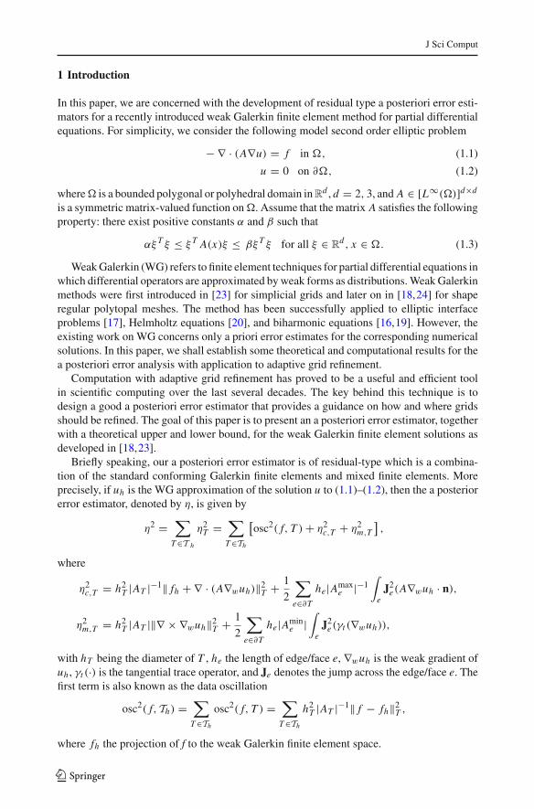
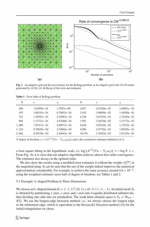
used, the error estimator contains simply the tangential jump of the weak derivative of uh .We present an adaptive grid generated by our algorithm in Fig. 1a and plot the decay rate of

the error as well as the estimator η in Fig. 1b. The approximated rate r is obtained by finding

123

J Sci Comput

102

103

104

102

101

100

Number of unknowns

Err

or

Rate of convergence is CN 0.56613

||Du Duh||

C1N 0.52043

etaC

2N 0.56613

(a) (b)

Fig. 1 An adaptive grid and the error history for the Kellogg problem. a An adaptive grid with 10,376 nodesgenerated by AFEM_WG. b Decay of the error and estimator

Table 1 Error table of Kellogg problem

N e η N e η

200 1.83099e−01 1.3987e+00 4,037 4.52260e−02 1.68851e−01

455 1.60243e−01 6.70852e−01 5,162 3.98050e−02 1.48580e−01

743 1.30391e−01 5.22967e−01 6,158 3.63765e−02 1.32420e−01

894 1.17721e−01 4.67049e−01 7,591 3.26328e−02 1.21772e−01

1, 009 1.07411e−01 4.09971e−01 8,654 3.05242e−02 1.13932e−01

1, 210 9.30829e−02 3.52864e−01 9,096 2.97702e−02 1.08385e−01

2, 062 6.59239e−02 2.46943e−01 10,376 2.78425e−02 1.01355e−01

N degree of freedom, e = ‖A1/2(∇u − ∇w,huh)‖, and η the a posteriori estimator defined in (4.1)

a least square fitting in the logarithmic scale, i.e. log ‖A1/2(∇u − ∇wuh)‖ ≈ r log N + c.From Fig. 1b, it is clear that our adaptive algorithm achieves almost first order convergence.The estimator also decays in the optimal order.

We also show the results using a modified error estimator η̃ without the weight |Amine | in

the tangential jump. It can be seen that the use of the weight indeed improves the numericalapproximation considerably. For example, to achieve the same accuracy around 4.6 × 10−2,using the weighted estimator saves half of degree of freedom; see Tables 1 and 2.

5.2 Example: L-shaped Problem in Three Dimensions

We choose an L-shaped domain� = (−1, 1)3/(0, 1)×(0, 1)×(−1,−1). An initial mesh T0

is obtained by partitioning x-axes, y-axes, and z-axes into 4 equally distributed subintervals,then dividing one cube into six tetrahedron. The weak finite element space is Vh = W0,0 −RT0. We use the longest-edge bisection method; i.e., we always choose the longest edgeas the refinement edge, which is equivalent to the Kossaczký bisection method [14] for theinitial triangulation we chose.

123

J Sci Comput

Table 2 Error table for Kellogg problem

N e η̃ N e η̃

289 2.54850e−01 3.88835e−01 4,048 6.50579e−02 9.36614e−02

423 1.98394e−01 3.57294e−01 4,591 6.31056e−02 8.74870e−02

607 1.53291e−01 2.77124e−01 5,458 5.83596e−02 7.81750e−02

802 1.24548e−01 2.32392e−01 6,666 5.44374e−02 7.17687e−02

916 1.14234e−01 2.10528e−01 9,092 4.87604e−02 6.01197e−02

1,149 1.00426e−01 1.85962e−01 9,825 4.72077e−02 5.88379e−02

2,011 8.01611e−02 1.39326e−01 10,351 4.64879e−02 5.62424e−02

N degree of freedom, e = ‖A1/2(∇u − ∇w,huh)‖, and η̃ a variant of estimator (4.1) without weight

103

104

101

100

Number of unknowns

err

Rate of convergence is CN 0.31995

||Du Duh||

C1N 0.3201

etaC

2N 0.31995

(a) (b)

Fig. 2 An adaptive grid and the error history for the L-shape problem in three dimensions. a An adaptive gridgenerated by AFEM_WG. b Decay of the error and estimator

Table 3 Error table of the L-shape problem in three dimensions

N e η N e η

113 2.80997e−01 1.47589e+00 1,374 1.15270e−01 6.13495e−01

133 2.50932e−01 1.27877e+00 1,914 1.02298e−01 5.40045e−01

154 2.39392e−01 1.19578e+00 2,763 9.25623e−02 4.80238e−01

188 2.19841e−01 1.16370e+00 4,052 8.17900e−02 4.37118e−01

258 1.92732e−01 1.01342e+00 5,573 7.27413e−02 3.84206e−01

351 1.76494e−01 9.14528e−01 8,375 6.52928e−02 3.38291e−01

489 1.59540e−01 8.50567e−01 11,281 5.86513e−02 3.09448e−01

687 1.40592e−01 7.45588e−01 15,960 5.20083e−02 2.74171e−01

965 1.28852e−01 6.68246e−01 23,419 4.64729e−02 2.43616e−01

N degree of freedom, e = ‖A1/2(∇u − ∇w,huh)‖, and η the a posteriori estimator defined in (4.1)

123

J Sci Comput

We set A = I and chose the Dirichlet boundary condition and the source f = 0 so that

the exact solution is u = r23 sin( 2

3θ) in the cylindrical coordinate. The function u containsan edge-type singularity. Again, for this example, only the tangential jump ∇ ×∇wuh acrossfaces contributes to the error estimator η.

For quasi-uniform grids in three dimensions, h = O(N− 13 ). Therefore we expect the error

to satisfy ‖A12 (∇u − ∇w,huh)‖ ≤ C N− 1

3 which is indeed the case shown in Fig. 2b. Anadaptive grids with correctly refined along the singular edge is also presented in Fig. 2a.Selected error and estimator is summarized in Table 3.

References

1. Ainsworth, M.: Robust a posteriori error estimation for nonconforming finite element approximation.SIAM J. Numer. Anal. 42(6), 2320–2341 (2005)

2. Alonso, A.: Error estimators for a mixed method. Numer. Math. 74(4), 385–395 (1996)3. Carstensen, C.: A posteriori error estimate for the mixed finite element method. Math. Comput. 66,

465–476 (1997)4. Chen, L.: iFEM: An integrated finite element methods package in MATLAB. University of California at

Irvine, Technical Report (2009)5. Chen, L., Holst, M., Xu, J.: Convergence and optimality of adaptive mixed finite element methods. Math.

Comput. 78, 35–53 (2009)6. Chen, L., Yie, X., Wang, J., Wang, Y.: Multilevel preconditioners for weak Galerkin methods, In prepa-

ration (2013)7. Chen, Z., Dai, S.: On the efficiency of adaptive finite element methods for elliptic problems with discon-

tinuous coefficients. SIAM J. Sci. Comput. 24(2), 443–462 (2002)8. Dari, V., Duran, E., Padra, R.G., Vampa, C.: A posteriori error estimators for nonconforming finite element

methods. Math. Model. Numer. Anal. 30, 385–400 (1996)9. Dörfler, W.: A convergent adaptive algorithm for Poisson’s equation. SIAM J. Numer. Anal. 33, 1106–

1124 (1996)10. Dryja, M., Sarkis, M.V., Widlund, O.B.: Multilevel Schwarz methods for elliptic problems with discon-

tinuous coefficients in three dimensions. Numer. Math. 72(3), 313–348 (1996)11. Duran, R.G.: Mixed Finite Element Methods. Class Notes (2007)12. Girault, V., Raviart, P.: Finite Element Methods for Navier-Stokes Equations: Theory and Algorithms,

volume 5 of Springer Series in Computational Mathematics. Springer, Berlin (1986). 87:5222713. Kellogg, R.B.: On the Poisson equation with intersecting interfaces. Appl. Anal. 4(2), 101–129 (1974)14. Kossaczky, I.: A recursive approach to local mesh refinement in two and three dimensions. J. Comput.

Appl. Math. 55, 275–288 (1994)15. Mitchell, W.F.: A comparison of adaptive refinement techniques for elliptic problems. ACM Trans. Math.

Softw. 15(4), 326–347 (1989)16. Mu, L., Wang, J., Wang, Y., Ye, X.: A weak Galerkin mixed finite element method for Biharmonic

equations. arXiv:1210.3818 (2012)17. Mu, L., Wang, J., Wei, G., Ye, X., Zhao, S.: Weak Galerkin method for the elliptic interface problem. J.

Comput. Phys. doi:10.1016/j.jcp.2013.04.042 (2013)18. Mu, L., Wang, J., Ye, X.: A weak Galerkin finite element method with polynomial reduction.

arXiv:1304.6481 (2012)19. Mu, L., Wang, J., Ye, X., Zhang, S.: A C0-weak Galerkin finite element method for the biharmonic

equation. arXiv:1212.0250 (2012)20. Mu, L., Wang, J., Ye, X., Zhao, S.: Numerical studies on the weak Galerkin method for the Helmholtz

equation with large wave number. arXiv:1111.0671 (2011)21. Petzoldt, M.: A posteriori error estimators for elliptic equations with discontinuous coefficients. Adv.

Comput. Math. 16(1), 47–75 (2002)22. Verfürth, R.: A Review of a posteriori Error Estimation and Adaptive Mesh Refinement Techniques. Wiley

Teubner, Chichester and Newyork (1996)23. Wang, J., Ye, X.: A weak Galerkin finite element method for second-order elliptic problems. J. Comput.

Appl. Math. 241, 103–115 (2013)24. Wang, J., Ye, X.: A weak Galerkin mixed finite element method for second-order elliptic problems. Math.

Comp., to appear (2013)

123