Embed Size (px)
Citation preview

ELECTRONIC RESEARCH ARCHIVE doi:10.3934/era.2020097Volume 29, Number 1, March 2021 pp. 1897–1923
A WEAK GALERKIN FINITE ELEMENT METHOD FOR
NONLINEAR CONSERVATION LAWS
Xiu Ye∗
Department of Mathematics, University of Arkansas at Little RockLittle Rock, AR 72204, USA
Shangyou Zhang
Department of Mathematical Sciences, University of Delaware
Newark, DE 19716, USA
Peng Zhu
College of Mathematics, Physics and Information Engineering, Jiaxing UniversityJiaxing, Zhejiang 314001, China
Abstract. A weak Galerkin (WG) finite element method is presented for non-linear conservation laws. There are two built-in parameters in this WG frame-
work. Different choices of the parameters will lead to different approaches for
solving hyperbolic conservation laws. The convergence analysis is obtainedfor the forward Euler time discrete and the third order explicit TVDRK time
discrete WG schemes respectively. The theoretical results are verified by nu-
merical experiments.
1. Introduction. The nonlinear hyperbolic equation of conservation laws is con-sidered: seeking an unknown function u satisfying
ut + f(u)x = 0, (x, t) ∈ I × (0, T ], (1.1)
u(x, 0) = φ(x), x ∈ I, (1.2)
with I = (0, 1) and a periodic boundary condition. For simplicity, the nonlinearflux function f(u) is assumed to be smooth enough.
The Runge-Kutta discontinuous Galerkin (RKDG) method has been developedfor solving time-dependent nonlinear conservation laws [1, 2]. The RKDG method,by name, uses DG method for spacial discretization and explicit high order Runge-Kutta method for time discretizations. The stability and error analysis of the RKDGmethod has been studied in [22, 23] for the second and the third order explicit totalvariation diminishing Runge-Kutta method. A discontinuous Galerkin method withLagrange multiplier (DGLM) has been developed in [6, 7] for nonlinear conservationlaws with backward Euler method for time discretization. Lagrange multipliers areintroduced on each element so that they are the only globally coupled variables in
2020 Mathematics Subject Classification. Primary: 65N15, 65N30; Secondary: 35J50.Key words and phrases. Weak Galerkin, finite element methods, weak derivative, conservation
laws.The first author is supported in part by NSF grant DMS-1620016. The third author is supported
in part by Zhejiang provincial NSF of China grant LY19A010008.∗ Corresponding author: Xiu Ye.
1897

1898 XIU YE, SHANGYOU ZHANG AND PENG ZHU
the resulting system. The final global system of the DGLM has fewer numbers ofcoupled unknowns than the usual DG methods.
The most finite element methods for conservation law employ purely upwindor general monotone fluxes. In [11], discontinuous Galerkin methods using moregeneral upwind-biased numerical fluxes have been investigated for time-dependentlinear conservation laws. Optimal order of convergence rate has been obtained. Aspointed out in [11], purely upwind fluxes may be difficult to construct for complexsystems.
Weak Galerkin methods refer to general finite element techniques for partialdifferential equations and were first introduced in [18, 19] for second order ellipticequations. Weak Galerkin methods make use of discontinuous piecewise polynomialson finite element partitions with arbitrary shape of polygons and polyhedrons. Theweak Galerkin methods have been applied to solve various PDEs such as second or-der elliptic equations, biharmonic equations, Stokes equations, parabolic equations,second order hyperbolic equations, Maxwell’s equations and singularly perturbedconvection-diffusion-reaction problems [8, 9, 10, 12, 13, 14, 15, 16, 17, 19, 20]. Aleast-squares based weak Galerkin method is presented for stationary linear hyper-bolic equations [21].
The objective of this work is to develop a weak Galerkin finite element methodfor the time-dependent nonlinear conservation laws (1.1)-(1.2), with the explicitfirst order Euler method and the third order explicit TVD Runge-Kutta methodfor time discretization. Similar to [11], this new WG formulation provides a classof finite element methods featuring two built-in parameters λ1 and λ2. By tuningthese parameters, different schemes can be obtained for solving the problem (1.1)-(1.2) including purely upwinding scheme. However, unlike the method in [11], ournew WG method can be used for the time-dependent nonlinear conservation laws.The stability is derived for the semi-discretized WG method. For the forward Eulertime discrete WG method, the L2 error estimate of O(hk+
12 +τ) is derived in general
and convergence rate of O(hk+1 + τ) is obtained for some special combination ofthe parameters. The temporal-spatial CFL condition τ < Ch2 is necessary in theerror analysis for the first order forward Euler method. If the third order explicitTVDRK time discrete scheme [3] is used, the L2 error estimate of O(hk+
12 + τ3) is
proved under the CFL condition τ < Ch.The rest of the paper is organized as follows. In Section 2, a WG finite element is
proposed for spatial discretization. The stability is derived for semi-discretized WGmethod. The forward Euler time discretized WG scheme and its error analysis arepresented in Section 3. Error analysis of the WG method with third order explicitTVDRK time discretization can be found in Section 4. Numerical experiments arepresented in Section 5 to support the theoretical results. We end the paper with aconclusion.
The usual notation of norms in Sobolev spaces will be used. For any integers ≥ 0, let Hs(D) represent the well-known Sobolev space equipped with the norm‖·‖s,D, which consists of functions with (distributional) derivatives of order no morethan s in L2(Ω). Next, denote by (·, ·)D the scalar inner product on L2(D) and‖ · ‖D denotes the associated L2 norm. Furthermore, let ‖ · ‖∞,D be the norm onL∞(D). If D = I, we omit this subscript.

WG METHOD FOR NONLINEAR CONSERVATION LAWS 1899
2. Semi-discrete weak Galerkin scheme and its stability. In this section,we introduce a weak Galerkin finite element method for solving the model problem(1.1)-(1.2).
2.1. Semi-discrete WG scheme. Let Th = ∪Ni=1Ii with Ii = [xi− 12, xi+ 1
2] for
1 ≤ i ≤ N where
0 = x 12< x 3
2< · · · < xN+ 1
2= 1.
Define
hi = xi+ 12− xi− 1
2, 1 ≤ i ≤ N ; h = max
1≤i≤Nhi, ∂Ii = xi− 1
2 ∪ xi+ 1
2.
The weak Galerkin methods introduce a new way to define a function v, calledweak function, which allows v taking different forms in the interior and on theboundary of the element:
v =
v0, in Ii
0,
vb, on ∂Ii,
where Ii0 is the interior of Ii, where Ii is an element in Th. Since a weak function
v is formed by two parts v0 and vb, we write v as v = v0, vb in short withoutconfusion.
Denote by Pk(Ii) the set of polynomials on Ii with degree no more than k. LetVh be a weak Galerkin finite element space consisting of weak function v = v0, vbdefined as follows for k ≥ 1,
Vh = v = v0, vb : v0|Ii ∈ Pk(Ii), vb|∂Ii ∈ P0(∂Ii),
vb(0) = vb(1), i = 1, · · · , N. (2.1)
Denote by v(x−i+ 1
2
) and v(x+i+ 1
2
) the values of v at xi+ 12
from the left element Ii
and the right element Ii+1, respectively. Further, the jump of v at xi+ 12
is denoted
as [[v]]i+ 12
= v(x+i+ 1
2
)− v(x−i+ 1
2
).
For v, w ∈ Vh, we introduce some notations,
〈v, w〉∂Ii = v(x−i+ 1
2
)w(x−i+ 1
2
) + v(x+i− 1
2
)w(x+i− 1
2
),
〈v, w〉∂Th =
N∑i=1
〈v, w〉∂Ii ,
(v, w)Th =
N∑i=1
(v, w)Ii =
N∑i=1
∫Ii
vwdx.
For any v = v0, vb ∈ Vh, a weak derivative Dwf(v) ∈ Pk(Ii) for i = 1, · · · , Nsatisfies
(Dwf(v), w)Ii = −(f(v0), Dw)Ii + 〈f(vb), wn〉∂Ii , ∀w ∈ Pk(Ii), (2.2)
where n = −1 at xi− 12
and n = 1 at xi+ 12. Here Dw means the first order derivative
of w, i.e. Dw = w′.Then we introduce a stabilizer in Vh as follows:
sh(v, w) =N∑i=1
(〈λ1(v0 − vb), w0 − wb〉∂+Ii + 〈λ2(v0 − vb), w0 − wb〉∂−Ii), (2.3)

1900 XIU YE, SHANGYOU ZHANG AND PENG ZHU
where ∂+Ii = xi+ 12, ∂−Ii = xi− 1
2, and λ1 and λ2 are two parameters. Here v0(xi+ 1
2)
and w0(xi+ 12) are the left limit of v0(x) and w0(x) at xi+ 1
2respectively, and v0(xi− 1
2)
and w0(xi− 12) are the right limit of v0(x) and w0(x) at xi− 1
2respectively.
The following is the semi-discretized weak Galerkin method.
Algorithm 1 (SD-WG method). A numerical approximation for (1.1)-(1.2) canbe obtained by seeking uh(t) = u0(t), ub(t) ∈ Vh satisfying uh(0) = Q0φ and thefollowing equation,
(∂tu0, v0) + (Dwf(uh), v0)Th + sh(uh, v) = 0, ∀ v = v0, vb ∈ Vh, (2.4)
where Q0 is the L2 projection onto Pk(Ii) on each element Ii.
Let Ii and Ii+1 be the two intervals sharing xi+ 12. Define the average v on
xi+ 12
by
vi =λ1
λ1 + λ2v(x−
i+ 12
) +λ2
λ1 + λ2v(x+
i+ 12
),
and
v0 = v(0), vN = v(1).
Please note that the definition of average · above is different from the standarddefinition of average which is when λ1 = λ2.
Testing (2.4) by v = v0, vb such that v0 = 0 and vb = 1 at xi+ 12
and vb = 0
otherwise, we can easily obtain that at xi+ 12
ub(t) = u0(t). (2.5)
Remark 1 (Relation to the upwinding-type DG method). If f ′(u) > 0 and takingλ2 = 0, then ub = u−0 and sh(uh, vh) = 0. Thus, the WG scheme (2.4) reduces to
(∂tu0, v0)Ii − (f(u0), v′0)Ii + 〈f(u−0 ), v0n〉∂Ii = 0, 1 ≤ i ≤ N,
which is the classical upwinding type discontinuous Galerkin method for nonlinearconservation law.
Remark 2 (Relation to the upwinding-biased DG method). Considering a specialcase f(u) = u. Taking λ1 = λ2 = λ in (2.3), and denote by
u0 = (1
2+
1
4λ)u−0 + (
1
2− 1
4λ)u+0 ,
then the WG scheme (2.4) reduces to
(∂tu0, v0)Ii − (u0, v′0)Ii + (u0)i+1/2(v0)−i+1/2 − (u0)i−1/2(v0)+i−1/2 = 0, 1 ≤ i ≤ N,
which is the upwinding-biased DG method discussed in [11].
2.2. Stability of the semi-discrete WG scheme. In this subsection, we willstudy the stability of the semi-discrete WG scheme (2.4).
Lemma 2.1. Let α2 ≤ f ′(s) ≤ α1. If λ1 > α1/2 and λ2 > −α2/2, then forv = v0, vb ∈ Vh, there holds
(Dwf(v), v0)Th + sh(v, v) ≥ 0. (2.6)

WG METHOD FOR NONLINEAR CONSERVATION LAWS 1901
Proof. As [5], we introduce g′(s) = f(s), then
(f(v0), Dv0)Th =
N∑i=1
∫Ii
f(v0)Dv0dx =
N∑i=1
∫Ii
Dg(v0)dx
=
N∑i=1
(g(v0(x−i+ 1
2
))− g(v0(x+i− 1
2
)))
=
N∑i=1
∫ v0(x−i+1
2
)
vb(xi+12)
f(s)ds−N∑i=1
∫ v0(x+
i− 12
)
vb(xi− 12)
f(s)ds.
Since f(vb) and vb take single value on ∂Ii, the periodic boundary condition implies
N∑i=1
〈f(vb), vbn〉∂Ii = 0. (2.7)
Using the definition of the weak derivative (2.2), the mean value theory and theperiodic boundary condition that
(Dwf(v), v0)Th = −(f(v0), Dv0)Th + 〈f(vb), v0n〉∂Th
= −N∑i=1
∫ v0(x−i+1
2
)
vb(xi+12)
(f(s)− f(vb))ds+
N∑i=1
∫ v0(x+
i− 12
)
vb(xi− 12)
(f(s)− f(vb))ds
= −N∑i=1
∫ v0(x−i+1
2
)
vb(xi+12)
f ′(ξ1)(s− vb)ds+
N∑i=1
∫ v0(x+
i− 12
)
vb(xi− 12)
f ′(ξ2)(s− vb)ds
which implies
(Dwf(v), v0)Th ≥ −α1
2
N∑i=1
(v0(x−i+ 1
2
)− vb(xi+ 12))2
+α2
2
N∑i=1
(v0(x+i− 1
2
)− vb(xi− 12))2, (2.8)
and
(Dwf(v), v0)Th ≤ α
2(
N∑i=1
(v0(x−i+ 1
2
)− vb(xi+ 12))2
+
N∑i=1
(v0(x+i− 1
2
)− vb(xi− 12))2), (2.9)
where α = max|α1|, |α2|. The equation (2.8) gives
(Dwf(v), v0)Th + sh(v, v) ≥N∑i=1
(λ1 −α1
2)(v0(x−
i+ 12
)− vb(xi+ 12))2
+
N∑i=1
(λ2 +α2
2)(v0(x+
i− 12
)− vb(xi− 12))2
≥ 0.
We complete the proof.

1902 XIU YE, SHANGYOU ZHANG AND PENG ZHU
Define ‖v‖2 =∫Iv2dx. Then we have the following stability result.
Lemma 2.2 (Stability of the SD-WG method). Let uh = u0, ub ∈ Vh be thesolution of the semi-discrete WG scheme (2.4), then
‖u0(T )‖ ≤ ‖u0(0)‖. (2.10)
Proof. Let v = uh in the semi-discrete WG scheme (2.4). From (2.6), we have
1
2
d
dt‖u0‖2 ≤ ((u0)t, u0) + (Dwf(uh), u0)Th + sh(uh, uh) = 0.
Integrating the above inequality with respect to time between 0 and T completesthe proof.
3. Forward Euler WG method and its error analysis. We use forward Eulermethod for time discretization to obtain a full discrete WG finite element method.
3.1. Forward Euler time discrete WG scheme. Let τ be a time step andtn = nτ .
Algorithm 2 (FE-WG method). Find un+1h = un+1
0 , un+1b ∈ Vh satisfying u0h =
Q0φ, Q0φ and
(un+10 − un0 , v0) + τ(Dwf(unh), v0)Th + τ sh(unh, v) = 0, ∀v ∈ Vh. (3.1)
Testing (3.1) by v = v0, vb such that v0 = 0 and vb = 1 at xi+ 12
and vb = 0
otherwise, we can easily obtain that at xi+ 12
unb = un0. (3.2)
We define a projection operator Qhu = Q0u,Qbu ∈ Vh, where Q0 is the L2
projection onto Pk(Ii) on each element Ii and Qbu = Q0u on ∂Ii.Define
enh = en0 , enb = Qhu(tn)− unh = Q0u(tn)− un0 , Qbu(tn)− unb , (3.3)
ρnh = ρn0 , ρnb = u(tn)−Qhu(tn) = u(tn)−Q0u(tn), u(tn)−Qbu(tn)(3.4)
and
`1(v) = (ut(tn)− u(tn+1)− u(tn)
τ, v0),
`2(v) = (Dwf(u(tn)), v0)Th − (Dwf(unh), v0)Th .
Lemma 3.1. The error function enh defined in (3.3) satisfies the following equation,
1
2‖en+1
0 ‖2 +1
2‖en+1
0 − en0‖2 −1
2‖en0‖2 + τ sh(enh, e
n+1h − enh) + τ sh(enh, e
nh)
+ τ`2(en+1h ) = −τ`1(en+1
h ) + τsh(Qhu(tn), en+1h ). (3.5)
Proof. Testing (1.1) by v0 of v = v0, vb ∈ Vh we arrive at
(ut, v0) + (Df(u), v0)Th = 0.
The definition of Dw implies,
(Df(u(tn)), v0)Th = (Dwf(u(tn)), v0)Th .
It follows from the definition of Q0 and the above equation,
(Q0u(tn+1)−Q0u(tn), v0) + τ(Dwf(u(tn)), v0)Th = −τ`1(v).

WG METHOD FOR NONLINEAR CONSERVATION LAWS 1903
Adding τsh(Qhu(tn), v) to the both sides of the above equation implies
(Q0u(tn+1)−Q0u(tn), v0) + τ(Dwf(u(tn)), v0)Th + τsh(Qhu(tn), v)
= τsh(Qhu(tn), v)− τ`1(v).
The difference of (3.1) and the equation above yields
(en+10 − en0 , v0) + τ sh(enh, v) + τ(Dwf(u(tn)), v0)Th − τ(Dwf(unh), v0)Th (3.6)
= τsh(Qhu(tn), v)− τ`1(v).
Using the fact 2p(p− q) = p2 + (p− q)2 − q2 and letting v = en+1h , (3.6) becomes
1
2‖en+1
0 ‖2 +1
2‖en+1
0 − en0‖2 −1
2‖en0‖2 + τsh(enh, e
n+1h − enh) + τ sh(enh, e
nh)
+ τ`2(en+1h ) = −τ`1(en+1
h ) + τsh(Qhu(tn), en+1h ).
We have proved the lemma.
3.2. Error analysis of forward Euler WG method. In this subsection we carryout an a priori error estimate for the fully discrete WG scheme with forward Eulertime marching for smooth solutions. We will assume the nonlinear flux functionf(u) is smooth enough for simplicity.
For any function ϕ ∈ H1(Ii), the following trace inequality holds true,
‖ϕ‖2∂Ii ≤ C(h−1i ‖ϕ‖
2Ii + hi‖∇ϕ‖2Ii
). (3.7)
Lemma 3.2. Let ρnh and enh be defined in (3.4) and (3.3) respectively. Then wehave
‖ρn0‖Ii ≤ Chk+1|u|k+1,Ii , ‖ρnb ‖∂Ii ≤ Chk+12 |u|k+1,Ii , (3.8)
‖enb ‖∂Ii ≤ Ch−1/2‖en0‖Ii . (3.9)
Proof. The first estimate in (3.8) is a direct result of the approximation property ofthe L2 projection Q0. The second estimate in (3.8) follows from the trace inequality(3.7) and the definitions of ρnb and Qh,
‖ρnb ‖∂Ii = ‖u(tn)−Qbu(tn)‖∂Ii = ‖u(tn)−Q0u(tn)‖∂Ii ≤ Chk+12 |u|k+1,Ii .
Similarly, we can prove (3.9).
Lemma 3.3. Let τ ≤ ch2. Then we have
τsh(Qhu(tn), en+1h ) ≤ Cτh2k+1|u|2k+1 + ε1‖en+1
0 − en0‖2 + ε2τsh(enh, enh), (3.10)
τ`1(en+1h ) ≤ Cτ3‖utt‖2 + ε1‖en+1
0 − en0‖2 + τ‖en0‖2, (3.11)
τsh(enh, en+1h − enh) ≤ Cτ‖en0‖2 + ε1‖en+1
0 − en0‖2. (3.12)

1904 XIU YE, SHANGYOU ZHANG AND PENG ZHU
Proof. It follows from (3.7), the Cauchy-Schwarz inequality and the definition ofQb that
sh(Qhu(tn), en+1h ) = sh(Qhu(tn), en+1
h − enh) + sh(Qhu(tn), enh)
=
N∑i=1
(〈λ1(Q0u(tn)− u(tn)), (en+10 − en0 )− (en+1
b − enb )〉∂+Ii
+ 〈λ2(Q0u(tn)− u(tn)), (en+10 − en0 )− (en+1
b − enb )〉∂−Ii)
+
N∑i=1
(〈λ1(Q0u(tn)− u(tn)), en0 − enb 〉∂+Ii
+ 〈λ2(Q0u(tn)− u(tn)), en0 − enb 〉∂−Ii)
≤ C(h−1hk+1|u|k+1‖en+10 − en0‖+ hk+
12 |u|k+1s
1/2h (enh, e
nh)).
Using the assumption τ ≤ ch2, we have
τsh(Qhu(tn), en+1h ) ≤ Cτ(h−1hk+1|u|k+1‖en+1
0 − en0‖+ hk+12 |u|k+1s
1/2h (enh, e
nh))
≤ C(ττ
h2h2k+2|u|2k+1 + τh2k+1|u|2k+1)
+ε1‖en+10 − en0‖2 + ε2τsh(enh, e
nh)
≤ Cτh2k+1|u|2k+1 + ε1‖en+10 − en0‖2 + ε2τsh(enh, e
nh),
which proves (3.10).It follows from the Cauchy-Schwarz inequality that
τ`1(en+1h ) ≤ Cτ2‖utt‖‖en+1
0 ‖≤ Cτ2‖utt‖(‖en+1
0 − en0‖+ ‖en0‖)≤ Cτ3‖utt‖2 + ε1‖en+1
0 − en0‖2 + τ‖en0‖2.
Using (3.7), Cauchy-Schwarz inequality, Lemma 3.2 and the assumption τ ≤ ch2,we have
τsh(enh, en+1h − enh) ≤ C τ
h‖en0‖‖en+1
0 − en0‖
≤ Cτ‖en0‖2 + ε1‖en+10 − en0‖2.
We have proved the lemma.
Lemma 3.4. For τ ≤ ch2 and λ1, λ2 ≥ α. Then we have
τ`2(en+1h ) ≤Cτh2k+1|u|2k+1 + Cτ‖en0‖2
+ ε1‖en+10 − en0‖2 + τ(
1
2+ ε2)sh(enh, e
nh). (3.13)
Proof. It follows from definition of the weak derivative Dw and the Taylor theory,
`2(en+1h ) =(Dwf(u(tn)), en+1
0 )Th − (Dwf(unh), en+10 )Th
=− (f(u(tn))− f(un0 ), Den+10 )Th + 〈f(u(tn))− f(unb ), en+1
0 n〉∂Th
=− (f ′(u(tn))(ρn0 + en0 ), Den+10 )Th +
1
2(f ′′(ξ1)(ρn0 + en0 )2, Den+1
0 )Th
+〈f ′(u(tn))(ρnb + enb ), en+10 n〉∂Th −
1
2〈f ′′(ξ2)(ρnb + enb )2, en+1
0 n〉∂Th
WG METHOD FOR NONLINEAR CONSERVATION LAWS 1905
=− (f ′(u(tn))ρn0 , Den+10 )Th + 〈f ′(u(tn))ρnb , e
n+10 n〉∂Th
+(−(f ′(u(tn))en0 , Den+10 )Th + 〈f ′(u(tn))enb , e
n+10 n〉∂Th)
+1
2(f ′′(ξ1)(ρn0 + en0 )2, Den+1
0 )Th −1
2〈f ′′(ξ2)(ρnb + enb )2, en+1
0 n〉∂Th
=
5∑i=1
Mi.
Next, we will bound all the terms above. Define f ′(u) = 1|Ii|∫Iif ′(u)dx. Using the
definitions of ρn0 and Q0, (3.8) and the inverse inequality, we arrive
M1 = (f ′(u(tn))ρn0 , Den+10 )Th
= ((f ′(u(tn))− f ′(u(tn)))ρn0 , Den+10 )Th
≤ Chk+1|u|k+1‖en+10 ‖
≤ Chk+1|u|k+1(‖en+10 − en0‖+ ‖en0‖).
It follows from the fact 〈f ′(u(tn))ρnb , enb n〉∂Th = 0, (3.7) and the inverse inequality,
M2 = 〈f ′(u(tn))ρnb , en+10 n〉∂Th
= 〈f ′(u(tn))ρnb , (en+10 − en0 )n〉∂Th + 〈f ′(u(tn))ρnb , (e
n0 − enb )n〉∂Th
≤ C(h−1hk+1|u|k+1‖en+10 − en0‖+ hk+
12 |u|k+1s
12
h (enh, enh)).
Using the inverse inequality, the trace inequality (3.7), (3.9) and (2.9), we obtain
M3 = −(f ′(u(tn))en0 , Den+10 )Th + 〈f ′(u(tn))enb , e
n+10 n〉∂Th
= −((f ′(u(tn))− f ′(u(tn)))en0 , Den+10 )Th + 〈(f ′(u(tn))− f ′(u(tn)))enb , e
n+10 n〉∂Th
− (f ′(u(tn))en0 , D(en+10 − en0 ))Th + 〈f ′(u(tn))enb , (e
n+10 − en0 )n〉∂Th
− (f ′(u(tn))en0 , Den0 )Th + 〈f ′(u(tn))enb , e
n0n〉∂Th
≤ C(‖en0‖2 + h−1‖en0‖‖en+10 − en0‖+
1
2sh(enh, e
nh)).
As [22, 23], we adopt the following a priori assumption to deal with the nonlinearityof the flux f(u)
‖en0‖ ≤ Ch3/2. (3.14)
And the justification of such assumption will be given in Remark 3. Then the aboveestimate with (3.2) gives
‖en0‖∞ ≤ Ch, ‖enb ‖∞ ≤ Ch. (3.15)
Using (3.8), (3.15) and the inverse inequality, we have
M4 =1
2(f ′′(ξ)(ρn0 + en0 )2, Den+1
0 )Th ≤ C(hk+1|u|k+1 + ‖en0‖)(‖en+10 − en0‖+ ‖en0‖),
M5 =1
2〈f ′′(ξ)(ρnb + enb )2, en+1
0 n〉∂Th ≤ C(hk+1|u|k+1 + ‖en0‖)(‖en+10 − en0‖+ ‖en0‖).
Combining all the estimates above gives
τ`2(en+1h ) ≤ Cτh2k+1|u|2k+1 + Cτ‖en0‖2 + ε1‖en+1
0 − en0‖2 + τ(1
2+ ε2)sh(enh, e
nh),
which proves the lemma.
1906 XIU YE, SHANGYOU ZHANG AND PENG ZHU
Theorem 3.5. Let un+1h ∈ Vh be the WG finite element solution of the problem
(1.1)-(1.2) arising from (3.1). Then there exists a constant C such that
‖en+10 ‖ ≤ C(hk+
12 |u|k+1 + τ‖utt‖).
Proof. It follows from (3.5) that
1
2‖en+1
0 ‖2 +1
2‖en+1
0 − en0‖2 −1
2‖en0‖2 + τ sh(enh, e
n+1h − enh) + τ sh(enh, e
nh)
+ τ`2(en+1h ) = −τ`1(en+1
h ) + τsh(Qhu(tn), en+1h ).
Then using Lemma 3.3 and Lemma 3.4, we have
1
2‖en+1
0 ‖2 + (1
2− 4ε1)‖en+1
0 − en0‖2 −1
2‖en0‖2 + (1− 1
2− 2ε2)sh(enh, e
nh)
≤ Cτh2k+1|u|2k+1 + Cτ‖en0‖2 + Cτ3‖utt‖2.
Letting ε1 and ε2 small enough gives
1
2‖en+1
0 ‖2 − 1
2‖en0‖2 ≤ Cτh2k+1|u|2k+1 + Cτ‖en0‖2 + Cτ3‖utt‖2.
Summing the above equation over n+ 1, we have
‖en+10 ‖2 ≤ ‖e00‖2 + Ch2k+1|u|2k+1 + Cτ2‖utt‖2 +
n∑i=0
Cτ‖ei0‖2.
The discrete Gronwall’s inequality implies
‖en+10 ‖2 ≤ C(h2k+1|u|2k+1 + τ2‖utt‖2),
which proves the theorem.
Remark 3. The assumption (3.14) is obviously satisfied for n = 0 since u00 = Q0φ.If (3.14) holds for a certain n, then it follows from the conclusion of Theorem 3.5and τ ≤ ch2 that
‖en+10 ‖ ≤ C(hk+1/2 + τ) ≤ Ch3/2,
for k ≥ 1. Thus the given a priori (3.14) is verified.
The result in the following theorem is a special case of Theorem 3.5. We omitthe proof of the theorem since it is similar to the proof of Theorem 3.5.
Theorem 3.6. Let un+1h ∈ Vh be the WG finite element solution of the problem
(1.1)-(1.2) arising from (3.1). Assume f ′(u) > 0 (or f ′(u) < 0) and let λ2 = 0 (orλ1 = 0). Then there exists a constant C such that
‖en+10 ‖ ≤ C(hk+1|u|k+1 + τ‖utt‖).
4. TVDRK3 WG method and its error analysis. This section discusses thefully discrete WG method coupled with the explicit TVDRK3 time-marching.
First, we set the initial value u0h = Q0φ, Q0φ. Then for each n ≥ 0, theapproximate solution from the time nτ to the next time (n + 1)τ is defined asfollows:
WG METHOD FOR NONLINEAR CONSERVATION LAWS 1907
Algorithm 3 (RK3-WG method). Find un,1h = un,10 , un,1b , un,2h = un,20 , un,2b
and un+1h = un+1
0 , un+1b in the finite element space Vh such that, for any v ∈ Vh
(un,10 − un0 , v0) + τ(Dwf(unh), v0)Th + τ sh(unh, v) = 0, (4.1)
(un,20 − 1
4un,10 − 3
4un0 , v0) +
1
4τ(Dwf(un,1h ), v0)Th +
1
4τ sh(un,1h , v) = 0, (4.2)
(un+10 − 2
3un,20 − 1
3un0 , v0) +
2
3τ(Dwf(un,2h ), v0)Th +
2
3τ sh(un,2h , v) = 0. (4.3)
Similar as (3.2), we obtain the time update for ub as
un,1b = un,10 , un,2b = un,20 , un+1b = un+1
0 . (4.4)
Following [22], two reference functions are defined in parallel to the TVDRK3time discretization stages for the exact solution of the conservation law (1.1). Letu(0)(x, t) = u(x, t) and
u(1)(x, t)− u(0)(x, t) + τ [f(u0(x, t))]x = 0, (4.5)
u(2)(x, t)− 1
4u(1)(x, t)− 3
4u(0)(x, t) +
1
4τ [f(u(1))(x, t)]x = 0. (4.6)
Lemma 4.1 ([23]). If ‖utttt‖ is bounded uniformly for any t ∈ [0, T ], we have
u(x, t+ τ)− 2
3u(2)(x, t)− 1
3u(0)(x, t) +
2
3τ [f(u(2))(x, t)]x = E(x, t), (4.7)
where E(x, t) is the local truncation error in time and ‖E(x, t)‖ = O(τ4) uniformlyfor any time t ∈ [0, T ].
Denote un,i = u(i)(x, tn) for any time level n and i = 0, 1, 2. The error at eachstage is denote by
en,ih = Qhun,i − un,ih , ρn,ih = un,i −Qhun,i
for any n and inner state i = 0, 1, 2, where un,0h = unh.
Lemma 4.2 (Error equation). For any v ∈ Vh, the error functions en,1h , en,2h and
en+1h satisfy the following equations
(en,10 , v0) = (en0 , v0) + τH(un, unh; v), (4.8)
(en,20 , v0) =3
4(en0 , v0) +
1
4(en,10 , v0) +
1
4τH(un,1, un,1h ; v), (4.9)
(en+10 , v0) =
1
3(en0 , v0) +
2
3(en,20 , v0) +
2
3τH(un,2, un,2h ; v) + (E , v0), (4.10)
where
H(u, uh; v) := (Dwf(uh)−Dwf(u), v0)Th + sh(uh, vh). (4.11)
Proof. Let t = tn and test (4.5) by v0 of v = v0, vb in Vh, we arrive at
(un,1 − un, v0) + τ(Df(un), v0)Th = 0.
The definition of Dw implies
(Df(un), v0)Th = (Dwf(un), v0)Th .
It follows from the definition of Q0 and the above equation that
(Q0un,1 −Q0u
n, v0) + τ(Dwf(un), v0)Th = 0.
The difference of (4.1) and the equation above yields (4.8).

1908 XIU YE, SHANGYOU ZHANG AND PENG ZHU
The error equations (4.9) and (4.10) can be obtained similarly. The details aretherefore omitted.
4.1. Some basic estimates. For any uh = u0, ub and vh = v0, vb in Vh, itfollows from the definition of weak derivative Dw that
(Dwf(uh)−Dwf(u), v0)Th
= (f(u)− f(u0), Dv0)Th − 〈f(u)− f(ub), v0n〉∂Th= (Ri(u, uh), Dv0)Th − 〈Rb(u, uh), v0n〉∂Th
+ (f ′(u)(u− u0), Dv0)Th − 〈f ′(u)(u− ub), v0n〉∂Th ,
where
Ri(u, uh) := f(u)− f(u0)− f ′(u)(u− u0),
Rb(u, uh) := f(u)− f(ub)− f ′(u)(u− ub).
Since Rb(u, u0) and f ′(u)(u − ub) take single value on ∂Ii, the periodic boundarycondition implies
−〈Rb(u, uh), v0n〉∂Th =
N∑j=1
Rb(u, uh)j+1/2[[v0]]j+1/2,
−〈f ′(u)(u− ub), v0n〉∂Th =
N∑j=1
(f ′(u)(u− ub))j+1/2[[v0]]j+1/2.
Therefore, the operator H(u, uh; vh) defined in (4.11) can be rewritten as
H(u, uh; vh) = Hlin(f ′(u);u− u0, v0) +Hnls(u, uh; vh) + sh(uh, vh), (4.12)
for uh, vh ∈ Vh, where
Hlin(Z; v, w) = (Zv,Dw)Th +
N∑j=1
(Zv[[w]])j+1/2,
Hnls(u, uh; vh) = (Ri(u, uh), Dv0)Th +
N∑j=1
Rb(u, uh)j+1/2[[v0]]j+1/2.
Lemma 4.3. For any continuous and differentiable function Z, there exists a pos-itive constant C, independent of n, h, τ , and uh, such that
|Hlin(Z; v, w)| ≤ Ch−1‖Z‖∞‖v‖‖w‖, ∀v, w ∈ Vh, (4.13)
|Hlin(Z; v, v)| ≤ C‖v‖2, ∀v ∈ Vh, (4.14)
|Hlin(Z;u−Q0u, v)| ≤ ε|Z|[[v]]2
+ ε‖v‖2 + Ch2k+1, ∀v ∈ Vh, (4.15)
where ε is any positive constant, and |Z|[[v]]2
=∑Nj=1 |Zj+1/2|[[v]]
2j+1/2.
Proof. For the proof of (4.13), it follows from Cauchy-Schwartz inequality and theinverse inequality that
|Hlin(Z; v, w)| ≤N∑j=1
(|(Zv,Dw)Ij |+ |Z|j+1/2|v|j+1/2|[[w]]|j+1/2)
WG METHOD FOR NONLINEAR CONSERVATION LAWS 1909
≤N∑j=1
‖Z‖∞(‖v‖Ij‖Dw‖Ij + ‖v‖∂Ij‖w‖∂Ij )
≤ Ch−1‖Z‖∞‖v‖‖w‖.
A simple manipulation indicates that
Hlin(Z; v, v) = (Zv,Dv)Th +
N∑j=1
(Zv[[v]])j+1/2
=
N∑j=1
(Zv[[v]]− 1
2Z[[v]]
2)j+1/2 −
∫ThZ ′v2dx
= −∫ThZ ′v2dx,
which implies the second conclusion (4.14).Let Zj = 1
|Ij |∫IjZdx. It follows from Cauchy-Schwartz inequality and Young’s
inequality that
Hlin(Z;u−Q0u, v) = (Z(u−Q0u), Dv)Th +
N∑j=1
(Zu−Q0u[[v]])j+1/2
=
N∑j=1
((Z − Zj)(u−Q0u), Dv)Ij +
N∑j=1
(Zu−Q0u[[v]])j+1/2
≤N∑j=1
‖Z − Zj‖L∞(Ij)‖u−Q0u‖Ij‖Dv‖Ij
+
N∑j=1
|Zj+1/2|‖u−Q0u‖L∞(Ij)|[[v]]|j+1/2
≤ ε‖v‖2 + ε
N∑j=1
|Zj+1/2|[[v]]2j+1/2 + Ch2k+1.
The proof is completed.
Lemma 4.4. Let u ∈ Hk+1(I) be the exact solution of (1.1). For any uh =u0, u0, vh = v0, v0 ∈ Vh, there holds
|Hnls(u, uh; vh)| ≤ C[‖v0‖2 + h−2‖u− u0‖2∞(‖Q0u− u0‖2 + h2(k+1))].
Proof. By Taylor expansion up to the second order derivative term, we obtain
Ri(u, uh) = −1
2f ′′(ξ1)(u− u0)2, Rb(u, uh) = −1
2f ′′(ξ2)u− u02,
where f ′′(ξ1) and f ′′(ξ2) are the second order derivative of f in the two expansion,which are both bounded.
Thus, by the triangle inequality and the inverse inequality, we have
|Hnls(u, uh; vh)| ≤1
2
N∑j=1
∣∣∣∣∣∫Ij
f ′′(ξ1)(u− u0)2Dv0dx
∣∣∣∣∣

1910 XIU YE, SHANGYOU ZHANG AND PENG ZHU
+1
2
N∑j=1
∣∣∣f ′′(ξ2)u− u02∣∣∣j+1/2
|[[v0]]|j+1/2
≤C‖u− u0‖∞N∑j=1
(‖u− u0‖Ij‖Dv0‖Ij + ‖u− u0‖∂Ij‖v0‖∂Ij )
≤C‖u− u0‖∞N∑j=1
[(‖u−Q0u‖Ij + ‖Q0u− u0‖Ij ) · h−1‖v0‖Ij
+ (‖u−Q0u‖L∞(Ij) + h−1/2‖Q0u− u0‖Ij ) · h−1/2‖v0‖Ij ]
≤Ch−1‖u− u0‖∞(‖Q0u− u0‖+ hk+1)‖v0‖,
which together with Young’s inequality completes the proof.
Lemma 4.5. Let u ∈ Hk+1(I) be the exact solution of (1.1). For any uh =u0, u0, vh = v0, v0 ∈ Vh, there hold
|sh(uh, vh)| ≤ Ch−1(hk+1 + ‖Q0u− u0‖)‖v0‖, (4.16)
sh(uh, eh) ≤ Ch2k+1 − (1− ε)ϑ[[e0]]2, (4.17)
where ε is any positive constant, [[e0]]2
:=∑Nj=1 [[e0]]
2j+ 1
2, and ϑ = λ1λ2
λ1+λ2.
Proof. Since u is continuous function, there holds [[u]] = 0. It follows from (2.3) and(4.4) that
sh(uh, vh) =
N∑j=1
ϑ[[u0]]j+1/2[[v0]]j+1/2 =
N∑j=1
ϑ[[u0 − u]]j+1/2[[v0]]j+1/2. (4.18)
Hence, by the triangle inequality and the inverse inequality, we have
|sh(uh, vh)| ≤CN∑j=1
|[[u0 − u]]|j+1/2|[[v0]]|j+1/2
≤CN∑j=1
(‖u−Q0u‖L∞(Ij) + h−1/2‖Q0u− u0‖Ij ) · h−1/2‖v0‖Ij
≤Ch−1(hk+1 + ‖Q0u− u0‖)‖v0‖,
which completed the proof of (4.16).From (4.18) and Young’s inequality, we have
sh(uh, eh) =
N∑j=1
ϑ[[Q0u− u]]j+1/2[[e0]]j+1/2 −N∑j=1
ϑ[[e0]]2j+1/2
≤ 1
4ε
N∑j=1
ϑ[[Q0u− u]]2j+1/2 − (1− ε)
N∑j=1
ϑ[[e0]]2j+1/2
≤Ch2k+1 − (1− ε)N∑j=1
ϑ[[e0]]2j+1/2.
The proof is completed.

WG METHOD FOR NONLINEAR CONSERVATION LAWS 1911
Lemma 4.6. If the time step satisfies τ = O(h), then we have
‖en,10 ‖2 ≤ C(‖en0‖2 + h2k+2), (4.19)
‖en,20 ‖2 ≤ C(‖en0‖2 + ‖en,10 ‖2 + h2k+2), (4.20)
where C is a positive constant independent of n, h, τ and uh.
Proof. Taking v = en,1h in the error equation (4.8), we get
‖en,10 ‖2 = (en0 , en,10 ) + τH(un, unh; en,1h ). (4.21)
Firstly, we consider the first term of H(un, unh; en,1h ). It follows from the definitionof the weak derivative Dw that
(Dwf(unh)−Dwf(un), en,10 )Th
= (f(un)− f(un0 ), Den,10 )Th − 〈f(un)− f(un0), en,10 n〉∂Th
=: T1 + T2. (4.22)
From Cauchy-Schwarz inequality, the inverse inequality and the approximationproperty of Q0, we have
|T1| ≤N∑j=1
‖f(un)− f(un0 )‖Ij‖Den,10 ‖Ij
≤ CN∑j=1
(‖un −Q0un‖Ij + ‖Q0u
n − un0‖Ij ) · h−1‖en,10 ‖Ij
≤ Ch−1(hk+1 + ‖en0‖)‖en,10 ‖, (4.23)
where the assumption f ′(u) is bounded has been used in the second inequalityabove.
Now we turn to the term T2. Since periodic boundary condition is considered,T2 can be rewritten as
T2 =
N∑j=1
(f(un)− f(un0))j+1/2[[en,10 ]]j+1/2.
Then, by the triangle inequality and the inverse inequality, we obtain
|T2| ≤ CN∑j=1
(|un −Q0un|+ |Q0u
n − un0|)j+1/2|[[en,10 ]]|j+1/2
≤ CN∑j=1
(‖un −Q0un‖L∞(Ij) + h−1/2‖Q0u
n − un0‖Ij ) · h−1/2‖en,10 ‖Ij
≤ Ch−1(hk+1 + ‖en0‖)‖en,10 ‖. (4.24)
Collecting (4.22), (4.23) and (4.24), we can conclude
|(Dwf(unh)−Dwf(un), en0 )Th | ≤ Ch−1(hk+1 + ‖en0‖)‖en,10 ‖,
which together with the inequality (4.16) of Lemma 4.5 and (4.21) yields
‖en,10 ‖2 ≤ ‖en0‖‖en,10 ‖+ Cτh−1(hk+1 + ‖en0‖)‖e
n,10 ‖.
1912 XIU YE, SHANGYOU ZHANG AND PENG ZHU
Cancelling ‖en,10 ‖ on both sides of the above equation, and noting that τ = O(h),we have
‖en,10 ‖ ≤ C(‖en0‖+ hk+1),
which implies (4.19).In a similar way, we can obtain the conclusion (4.20). The proof is completed.
By taking the test function v = enh, 4en,1h , and 6en,2h in the error equations (4.8),
(4.9) and (4.10), respectively, we obtain the energy equation for enh in the form
3‖en+10 ‖2 − 3‖en0‖2 = Ξ1 + Ξ2, (4.25)
where
Ξ1 :=τH(un, unh; enh) + τH(un,1, un,1h ; en,1h ) + 4τH(un,2, un,2h ; en,2h ) + 6(E , en,20 ),
Ξ2 :=‖2en,20 − en,10 − en0‖2 + 3(en+10 − en0 , en+1
0 − 2en,20 + en0 ).
4.2. The estimate for Ξ1. It follows from (4.14) and (4.15) of Lemma 4.3 that
Hlin(f ′(un);un − unh, en0 ) = Hlin(f ′(un);un −Q0un, en0 ) +Hlin(f ′(un); en0 , e
n0 )
≤ ε|f ′(un)|[[en0 ]]2
+ (ε+ C)‖en0‖2 + Ch2k+1.
Denote by B = maxs∈R |f ′(s)|. In the above inequality, taking ε small enough suchthat εB ≤ 0.1ϑ, then we have
Hlin(f ′(un);un − unh, en0 ) ≤ 0.1ϑ[[en0 ]]2
+ C‖en0‖2 + Ch2k+1. (4.26)
From Lemma 4.4, we have
Hnls(un, unh; enh) ≤ C[‖en0‖2 + h−2‖un − un0‖2∞(‖en0‖2 + h2(k+1))]. (4.27)
Using (4.17) of Lemma 4.5 with ε = 0.1, we have
sh(unh, enh) ≤ Ch2k+1 − 0.9ϑ[[en0 ]]
2. (4.28)
Denote by
C(un,i, un,i0 ) = C(1 + h−2‖un,i − un,i0 ‖2∞), i = 0, 1, 2,
where C is a general positive constant independent of h, τ, u and uh. Collecting(4.26), (4.27) and (4.28), we obtain
H(un, unh; enh) ≤ C(un, un0 )(‖en0‖2 + h2k+1)− 0.8ϑ[[en0 ]]2.
Similarly, we have
H(un,i, un,ih ; en,ih ) ≤ C(un,i, un,i0 )(‖en,i0 ‖2 + h2k+1)− 0.8ϑ[[en,i0 ]]2,
for i = 1, 2.Since E = O(τ4), by Cauchy-Schwartz inequality, we have
(E , en,20 ) ≤ ‖E‖‖en,20 ‖ ≤ Cτ4‖en,20 ‖ ≤ C(τ7 + τ‖en,20 ‖2).
Collecting the three above estimates, we obtain the estimate of Ξ1 as follows
Ξ1 ≤ τ2∑i=0
C(un,i, un,i0 )(‖en,i0 ‖2 + h2k+1)− 0.8ϑ[[en,i0 ]]2+ Cτ7. (4.29)

WG METHOD FOR NONLINEAR CONSERVATION LAWS 1913
4.3. The estimate for Ξ2. Following [23], we introduce the following notations
Enh = en,1h − enh, Fnh = 2en,2h − en,1h − enh, Gnh = en+1h − 2en,2h + enh.
Obviously,
en,20 − 3
4en0 −
1
4en,10 =
1
4En0 +
1
2Fn0 ,
en+10 − 1
3en0 −
2
3en,20 =
2
3En0 +
2
3Fn0 +Gn0 .
From the above equalities and the error equations (4.8)-(4.10), we easily obtain thefollowing results.
Lemma 4.7. For the fully discrete WG method (4.1)-(4.3) with the explicit TV-DRK3 time marching, we have the following equations
(En0 , v0) = τH(un, unh; vh), (4.30)
(Fn0 , v0) =τ
2[H(un,1, un,1h ; vh)−H(un, unh; vh)], (4.31)
(Gn0 , v0) =τ
3[2H(un,2, un,2h ; vh)−H(un,1, un,1h ; vh)−H(un, unh; vh)] + (E , v0),
(4.32)
for any vh = v0, vb ∈ Vh.
Note that en+10 − en0 = En0 + Fn0 +Gn0 , there holds
Ξ2 =(Fn0 , Fn0 ) + 3(En0 , G
n0 ) + 3(Fn0 , G
n0 ) + 3(Gn0 , G
n0 )
:=J1 + J2 + J3 + J4. (4.33)
Let vh = Fnh in (4.31) and vh = Enh in (4.32), and by (4.12), we have
J1 + J2 =− (Fn0 , Fn0 ) + 2(Fn0 , F
n0 ) + 3(En0 , G
n0 )
=− ‖Fn0 ‖2 + τ [H(un,1, un,1h ;Fnh )−H(un, unh;Fnh )]
+ τ [2H(un,2, un,2h ;Enh )−H(un,1, un,1h ;Enh )−H(un, unh;Enh )] + 3(E , En0 )
=− ‖Fn0 ‖2 +
3∑i=1
Mi + 3(E , En0 ), (4.34)
where
M1 :=τ [Hlin(f ′(un,1);un,1 − un,10 , Fn0 )−Hlin(f ′(un);un − un0 , Fn0 )]
+ τ [2Hlin(f ′(un,2);un,2 − un,20 , En0 )−Hlin(f ′(un,1);un,1 − un,10 , En0 )
−Hlin(f ′(un);un − un0 , En0 )],
M2 :=τ [Hnls(un,1, un,1h ;Fnh )−Hnls(un, unh;Fnh )]
+ τ [2Hnls(un,2, un,2h ;Enh )−Hnls(un,1, un,1h ;Enh )−Hnls(un, unh;Enh )],
M3 :=τ [sh(un,1h − unh, Fnh ) + sh(2un,2h − un,1h − unh, Enh )].
Lemma 4.8 (Estimate of M1). If the time step satisfies τ = O(h), then we have
|M1| ≤ Cτ(‖en,20 ‖2 + ‖en,10 ‖2 + ‖en0‖2 + h2(k+1)).
Proof. Since un,i − un,ih = ρn,ih + en,ih (i = 0, 1, 2), then M1 can be rewritten as
M1 = τ [L(ρh) + L(eh)], (4.35)

1914 XIU YE, SHANGYOU ZHANG AND PENG ZHU
where
L(w) =Hlin(f ′(un,1);wn,1, Fn0 )−Hlin(f ′(un);wn, Fn0 )
+ 2Hlin(f ′(un,2);wn,2, En0 )−Hlin(f ′(un,1);wn,1, En0 )
−Hlin(f ′(un);wn, En0 ),
for w = ρh or eh.Denote by
zn,i = f ′(un,i)− f ′(un), i = 1, 2,
and collecting the terms with the same speed f ′(un), the operator L(w) can beexpressed as
L(w) =Hlin(f ′(un);wn,1 − wn, Fn0 ) +Hlin(f ′(un); 2wn,2 − wn,1 − wn, En0 )
+Hlin(zn,1;wn,1, Fn0 ) + 2Hlin(zn,2;wn,2, En0 )−Hlin(zn,1;wn,1, En0 )
:=
5∑i=1
Li(w).
Now we estimate Li(eh), i = 1, · · · , 5 firstly. Due to periodic boundary condition,and using integration by parts, we have
L1(eh) + L2(eh) = Hlin(f ′(un); en,1h , Fn0 ) +Hlin(f ′(un); en,2h , En0 )
=
N∑j=1
[
∫Ij
f ′(un)(En0 Fn0 )xdx+ f ′(un)j+1/2[[En0 F
n0 ]]j+1/2]
=
N∑j=1
∫Ij
−[f ′(un)]xEn0 F
n0 dx.
Consequently, by Cauchy-Schwartz inequality, we can conclude that
|L1(eh) + L2(eh)| ≤ C‖En0 ‖‖Fn0 ‖.
Since |zn,1| = O(τ) = O(h), it follows from the equation (4.13) of Lemma 4.3 that
|L3(eh)| = |Hlin(zn,1; en,1h , Fn0 )|
≤ Ch−1‖zn,1‖∞‖en,10 ‖‖Fn0 ‖
≤ C‖en,10 ‖‖Fn0 ‖.
In a similar way, we obtain
|L4(eh)|+ |L5(eh)| ≤ C(‖en,20 ‖+ ‖en,10 ‖)‖En0 ‖.
Collecting the estimate of Li(eh), i = 1, · · · , 5 and using Cauchy-Schwarz inequalityyields
|L(eh)| ≤ C(‖En0 ‖2 + ‖Fn0 ‖2 + ‖en,10 ‖2 + ‖en,20 ‖2). (4.36)
WG METHOD FOR NONLINEAR CONSERVATION LAWS 1915
Next, we turn to the term Li(ρh), i = 1, · · · , 5. Note that f ′(u) is bounded, itfollows from the Cauchy-Schwartz inequality and inverse equality that
|L1(ρh)| = |Hlin(f ′(un); ρn,10 − ρn0 , Fn0 )|
≤ CN∑j=1
‖f ′(un)‖∞(‖ρn,10 − ρn0‖Ij‖DFn0 ‖Ij + ‖ρn,10 − ρn0‖∂Ij‖Fn0 ‖∂Ij )
≤ C(h−1‖ρn,10 − ρn0‖+ h−1/2‖ρn,10 − ρn0‖∞)‖Fn0 ‖. (4.37)
Since
un,1 − un = −τ [f(un)]x,
it follows from the approximation property of L2 projector Q0 that
‖ρn,10 − ρn0‖ =‖(un,1 − un)−Q0(un,1 − un)‖ ≤ Chk+1τ,
‖ρn,10 − ρn0‖∞ =‖(un,1 − un)−Q0(un,1 − un)‖∞ ≤ Chk+1/2τ,
which together with (4.37) yields
|L1(ρh)| ≤ Chkτ‖Fn0 ‖ ≤ C(‖Fn0 ‖2 + h2kτ2).
Similarly we can estimate the second term as |L2(ρh)| ≤ C(‖En0 ‖2 + h2kτ2).Using |zn,i| = O(τ) = O(h) and similar as the proof of L1(ρh), it is easy to
obtain
|L3(ρh)|+ |L4(ρh)|+ |L5(ρh)| ≤ C(‖En0 ‖2 + ‖Fn0 ‖2 + h2(k+1)).
Since τ = O(h), finally we have
|L(ρh)| ≤ C(‖En0 ‖2 + ‖Fn0 ‖2 + h2(k+1)). (4.38)
By the triangle inequality, we have
‖En0 ‖2 + ‖Fn0 ‖2 ≤ C(‖en,20 ‖2 + ‖en,10 ‖2 + ‖en0‖2),
which together with (4.36) and (4.38) completes the proof.
Lemma 4.9 (Estimate ofM2). There exists a positive constant C, independent ofn, h, τ , and uh, such that
|M2| ≤ Cτ2∑i=0
[‖en,i0 ‖2 + h−2‖un,i − un,i0 ‖2∞(‖en,i0 ‖2 + h2(k+1))].
Proof. It follows from Lemma 4.4 that
|Hnls(un,i, un,ih ;wh)| ≤ C[‖w0‖2 + h−2‖un,i − un,i0 ‖2∞(‖en,i0 ‖2 + h2(k+1))],
for wh ∈ Vh and i = 0, 1, 2.Let wh = Enh and Fnh in the above inequality, respectively. By the triangle
inequality and the definition of M2, we have
|M2| ≤τ [|Hnls(un,1, un,1h ;Fnh )|+ |Hnls(un, unh;Fnh )|]
+ τ [2|Hnls(un,2, un,2h ;Enh )|+ |Hnls(un,1, un,1h ;Enh )|+ |Hnls(un, unh;Enh )|]
≤Cτ [‖En0 ‖2 + ‖Fn0 ‖2 +
2∑i=0
h−2‖un,i − un,i0 ‖2∞(‖en,i0 ‖2 + h2(k+1))],
which completes the proof.
1916 XIU YE, SHANGYOU ZHANG AND PENG ZHU
Lemma 4.10 (Estimate of M3). There exists a positive constant C, independentof n, h, τ , and uh, such that
|M3| ≤ Ch2k+1τ − 0.9ϑ([[En0 ]]2
+ [[Fn0 ]]2)τ.
Proof. Using (4.17) of Lemma 4.5 with ε = 0.1, we have
sh(un,1h − unh, Fnh ) ≤ Ch2k+1 − 0.9ϑ[[Fn0 ]]2,
sh(2un,2h − un,1h − unh, Enh ) ≤ Ch2k+1 − 0.9ϑ[[En0 ]]2.
Combining the above two estimates completes the proof.
Since E = O(τ4), by Cauchy-Schwartz inequality, we have
(E , En0 ) ≤ C(τ7 + τ‖En0 ‖2) ≤ C(τ7 + τ‖en0‖2 + τ‖en,10 ‖2),
which together with (4.34) and Lemma 4.8, 4.9 and 4.10 yields
J1 + J2 ≤ −‖Fn0 ‖2 + τ
2∑i=0
C(un,i, un,i0 )(‖en,i0 ‖2 + h2k+1)
+Cτ7 − 0.9ϑ([[En0 ]]2
+ [[Fn0 ]]2)τ. (4.39)
Now we consider the upper bound of J3 and J4. Since J3 = 3(Gn0 , Fn0 ) and
J4 = 3(Gn0 , Gn0 ), we estimate 3(Gn0 , v0) in general. From (4.12) and (4.32), we have
3(Gn0 , v0) =τ [2H(un,2, un,2h ; vh)−H(un,1, un,1h ; vh)−H(un, unh; vh)] + 3(E , v0)
:=τ [I1(v0) + I2(v0) + I3(v0)] + 3(E , v0), (4.40)
where
I1(v0) :=2Hlin(f ′(un,2);un,2 − un,20 , v0)−Hlin(f ′(un,1);un,1 − un,10 , v0)
−Hlin(f ′(un);un − un0 , v0),
I2(v0) :=2Hnls(un,2, un,2h ; vh)−Hnls(un,1, un,1h ; vh)−Hnls(un, unh; vh),
I3(v0) :=2sh(un,2h , vh)− sh(un,1h , vh)− sh(unh, vh).
Denote by
Fn0 := 2ρn,20 − ρn,10 − ρn0 ,and collecting the terms with the same speed f ′(un), we rewrite the operator I1(v0)as
I1(v0) :=Hlin(f ′(un);Fn0 , v0) + 2Hlin(zn,2; en,20 , v0)−Hlin(zn,1; en,10 , v0)
+Hlin(f ′(un); Fn0 , v0) + 2Hlin(zn,2; ρn,20 , v0)−Hlin(zn,1; ρn,10 , v0)(4.41)
It follows from (4.13) of Lemma 4.3, Cauchy-Schwartz inequality and |zn,i| =O(τ) = O(h) that
|Hlin(f ′(un);Fn0 , v0)| ≤ Ch−1‖f ′(un)‖∞‖Fn0 ‖‖v0‖ ≤ Ch−1(‖Fn0 ‖2 + ‖v0‖2),(4.42)
|Hlin(zn,i; en,i0 , v0)| ≤ Ch−1‖zn,i‖∞‖en,i0 ‖‖v0‖ ≤ C(‖en,i0 ‖2 + ‖v0‖2), i = 1, 2.(4.43)

WG METHOD FOR NONLINEAR CONSERVATION LAWS 1917
Note that f ′(u) is bounded, it follows from the Cauchy-Schwartz inequality andinverse equality that
|Hlin(f ′(un); Fn0 , v0)| ≤N∑j=1
‖f ′(un)‖∞(‖Fn0 ‖Ij‖Dv0‖Ij + ‖Fn0 ‖∂Ij‖v0‖∂Ij )
≤ CN∑j=1
(h−1‖Fn0 ‖Ij + h−1/2‖Fn0 ‖∂Ij )‖v0‖Ij . (4.44)
Since
Fn0 = (2un,2 − un,1 − un)−Q0(2un,2 − un,1 − un)
and
2un,2 − un,1 − un =τ
2([f(un)]x − [f(un,1)]x),
by the approximation property of L2 projector Q0, we have
‖Fn0 ‖Ij ≤ Chk+1τ, ‖Fn0 ‖∂Ij ≤ Chk+1/2τ. (4.45)
Plugging (4.45) into (4.44), and using 2ab ≤ a2 + b2, we get
|Hlin(f ′(un); Fn0 , v0)| ≤ C(h2kτ2 + ‖v0‖2). (4.46)
Similar to the proof of (4.44), and note that |zn,i| = O(τ), we have
|Hlin(zn,i; ρn,i0 , v0)| ≤ C(h2kτ2 + ‖v0‖2), i = 1, 2. (4.47)
Combining (4.41), (4.42), (4.43), (4.46) and (4.47), and assume τ = O(h), we have
I1(v0) ≤ Ch−1(‖Fn0 ‖2 + ‖v0‖2) + C(‖en,10 ‖2 + ‖en,20 ‖2 + ‖v0‖2 + h2k+2). (4.48)
Thanks to Lemma 4.4, we have
I2(v0) ≤ C‖v0‖2 + C
2∑i=0
h−2‖un,i − un,i0 ‖2∞(‖en,i0 ‖2 + h2(k+1)). (4.49)
It follows from (4.18) and Young’s inequality that
I3(v0) = sh(2(un,2h − un,2)− (un,1h − un,1)− (unh − un), vh)
= −N∑j=1
ϑ[[Fn0 ]]j+1/2[[v0]]j+1/2 −N∑j=1
ϑ[[Fn0 ]]j+1/2[[v0]]j+1/2
≤ 1
4
N∑j=1
ϑ[[Fn0 ]]2j+1/2 + 2
N∑j=1
ϑ[[v0]]2j+1/2 +
1
4ϑ[[Fn0 ]]
2,
which together with (4.45) and inverse inequality yields
I3(v0) ≤ C(h2k+1τ + h−1‖v0‖2) +1
4ϑ[[Fn0 ]]
2. (4.50)
Using the fact E = O(τ4) and Cauchy-Schwartz inequality, we get
3(E , v0) ≤ C(τ7 + τ‖v0‖2),

1918 XIU YE, SHANGYOU ZHANG AND PENG ZHU
which combining with (4.48), (4.49), (4.50) and (4.40) yields
3(Gn0 , v0) ≤ Cτh−1(‖Fn0 ‖2 + ‖v0‖2) + Cτ‖v0‖2 +τ
4ϑ[[Fn0 ]]
2+ Cτ7
+τ
2∑i=0
C(un,i, un,i0 )(‖en,i0 ‖2 + h2(k+1)). (4.51)
Taking v0 = Fn0 in (4.51) and using the assumption τ ≤ γh, we have
J3 ≤ 2Cγ‖Fn0 ‖2 +τ
4ϑ[[Fn0 ]]
2+ Cτ7 + τ
2∑i=0
C(un,i, un,i0 )(‖en,i0 ‖2 + h2(k+1)). (4.52)
Taking v0 = Gn0 in (4.51), we have
3‖Gn0‖2 ≤Cγ‖Fn0 ‖2 + 2Cγ‖Gn0‖2 +τ
4ϑ[[Fn0 ]]
2+ Cτ7
+ τ
2∑i=0
C(un,i, un,i0 )(‖en,i0 ‖2 + h2(k+1)),
then
(3− 2Cγ)‖Gn0‖2 ≤Cγ‖Fn0 ‖2 +τ
4ϑ[[Fn0 ]]
2+ Cτ7
+ τ
2∑i=0
C(un,i, un,i0 )(‖en,i0 ‖2 + h2(k+1)).
Therefore,
J4 ≤3
3− 2Cγ[Cγ‖Fn0 ‖2 +
τ
4ϑ[[Fn0 ]]
2+ Cτ7
+τ
2∑i=0
C(un,i, un,i0 )(‖en,i0 ‖2 + h2(k+1))],
which combining with (4.52) yields
J3 + J4 ≤ (2Cγ +3Cγ
3− 2Cγ)‖Fn0 ‖2 +
1
4(1 +
3
3− 2Cγ)τϑ[[Fn0 ]]
2
+Cτ7 + τ
2∑i=0
C(un,i, un,i0 )(‖en,i0 ‖2 + h2(k+1)).
In the above inequality, taking τ small enough such that Cγ = 1/4, then we get
J3 + J4 ≤0.8‖Fn0 ‖2 + 0.55τϑ[[Fn0 ]]2
+ Cτ7
+ τ
2∑i=0
C(un,i, un,i0 )(‖en,i0 ‖2 + h2(k+1)),
which together with (4.39) and (4.33) yields
Ξ2 ≤− 0.2‖Fn0 ‖2 − τϑ(0.9[[En0 ]]2
+ 0.35[[Fn0 ]]2)
+ Cτ7 + τ
2∑i=0
C(un,i, un,i0 )(‖en,i0 ‖2 + h2(k+1)). (4.53)
WG METHOD FOR NONLINEAR CONSERVATION LAWS 1919
4.4. Main results. In this subsection, we will give the L2 norm error estimatebetween the exact solution u(tn) and the WG solution un0 .
Theorem 4.11. Let uh be the numerical solution of the fully discrete WG scheme(4.1)-(4.4) with the explicit TVDRK3 time marching. Let u be the exact solution ofproblem (1.1)-(1.2), where f(u) is smooth enough. If u and its spatial derivatives upto the second order are all continuous in I = (0, 1), and ‖u‖k+1, ‖ut‖k+1, ‖utt‖k+1
and ‖uttt‖k+1 are bounded uniformly for any time t ∈ (0, T ], then the followingerror estimate holds
‖u(tn)− un0‖ ≤ C(hk+1/2 + τ3) (4.54)
under the condition τ ≤ γh with a fixed constant γ > 0. Here C is a positiveconstant independent of h, τ and uh.
Proof. Denote by
∆ = 0.2‖Fn0 ‖2 + τϑ(0.9[[En0 ]]2
+ 0.35[[Fn0 ]]2
+ 0.8
2∑i=0
[[en,i0 ]]2),
then from (4.25), (4.29) and (4.53), we obtain
3‖en+10 ‖2 − 3‖en0‖2 + ∆ ≤ Cτ7 + τ
2∑i=0
C(un,i, un,i0 )(‖en,i0 ‖2 + h2k+1). (4.55)
As [22, 23], we adopt the following a priori assumption for m (mτ < T ) to dealwith the nonlinearity of the flux f(u)
‖en,i0 ‖ ≤ Ch3/2, for n ≤ m, i = 0, 1, 2. (4.56)
The justification of such assumption will be given later.It follows from the assumption (4.56) and the approximation property of L2
operator Q0
‖ρn,i0 ‖∞ = ‖un,i −Q0un,i‖∞ ≤ Chk+1/2, i = 0, 1, 2
implies that
‖un,i − un,i0 ‖∞ ≤ ‖ρn,i0 ‖∞ + Ch−1/2‖en,i0 ‖ ≤ Ch.
Therefore, we have
C(un,i, un,i0 ) ≤ C, for n ≤ m, i = 0, 1, 2,
which together with (4.55), (4.19) and (4.20) yields
3‖en+10 ‖2 − 3‖en0‖2 ≤ Cτ7 + C(‖en0‖2 + h2k+1)τ,
where C is a positive constant independent of m,n,h and τ . Then an application ofthe discrete Gronwall inequality yields
‖en+10 ‖2 ≤ C(τ6 + h2k+1), n ≤ m, (4.57)
which together with
‖ρn+10 ‖ = ‖un+1 −Q0u
n+1‖ ≤ Chk+1
yields that
‖un+1 − un+10 ‖ ≤ C(τ3 + hk+1/2).

1920 XIU YE, SHANGYOU ZHANG AND PENG ZHU
Now we turn to verify the reasonableness of the a priori assumption (4.56). Sincee00 = 0, by (4.19) and (4.20), we easily obtain
‖e0,i0 ‖ ≤ Chk+1 ≤ Ch3/2
for i = 0, 1, 2 and k ≥ 1. Supposing (4.56) holds for m, we can show that thisassumption is also true for m + 1. Inequality (4.57) as well as (4.19) and (4.20)imply that
‖em+1,i0 ‖ ≤ C(‖em+1
0 ‖+ hk+1) ≤ C(τ3 + hk+1/2) ≤ Ch3/2
for k ≥ 1 and i = 1, 2. Thus the assumption (4.56) is reasonable, and hence theabove error estimate holds for any m (mτ < T ). The proof is completed.
5. Numerical examples. In this section, we present the numerical examples toverify our theoretical findings. In our numerical experiments, we shall use piecewiseuniform meshes which are constructed by equally dividing spatial domain into Nsubintervals. The main purpose of this paper is to investigate how to use WGmethod to discretize spacial variables in conservation law. In order to reduce thetime errors, we use the third order explicit TVDRK time discrete scheme in time,and take time step τ = CFL ·h, where CFL is a constant independent of the meshsize h. WG scheme with Pk(k = 1, 2, 3) element is used for spatial discretization.
Example 1 (A smooth solution of a linear equation). We solve the followinglinear problem (1.1) with periodic boundary condition,
ut + ux = 0, (x, t) ∈ (0, 2π)× (0, T ],
u(x, 0) = sinx, x ∈ (0, 2π).
The exact solution to this problem is
u(x, t) = sin(x− t).
Let time step size τ = 0.05h in this example. WG scheme with Pk(k = 1, 2, 3) el-ement is used for spatial discretization. The L2 errors and the order of convergence,at T = 2π, are reported in Table 1. It is observed that the order of convergence ofthe L2 error achieves (k + 1)-th order of accuracy.
Table 1. L2 errors and corresponding convergence rates of Exam-ple 1. T = 2π, λ1 = λ2 = 1.
P1 element P2 element P3 elementN ‖u− u0‖ Rate ‖u− u0‖ Rate ‖u− u0‖ Rate8 1.29E-01 3.36E-03 2.66E-0416 3.02E-02 2.10 3.99E-04 3.08 1.94E-05 3.7832 7.22E-03 2.06 4.93E-05 3.02 1.27E-06 3.9364 1.78E-03 2.02 6.14E-06 3.00 8.06E-08 3.98128 4.42E-04 2.01 7.67E-07 3.00 5.06E-09 4.00
Example 2 (A blow-up solution of a nonlinear equation). We solve thefollowing nonlinear problem (1.1) with periodic boundary condition,
ut + (u2/2)x = 0, (x, t) ∈ (0, 1)× (0, T ],
u(x, 0) = φ(x), x ∈ (0, 1),
WG METHOD FOR NONLINEAR CONSERVATION LAWS 1921
0 0.2 0.4 0.6 0.8 1
-0.4
-0.2
0
0.2
0.4
0.6
0.8
WG solution
Exact solution
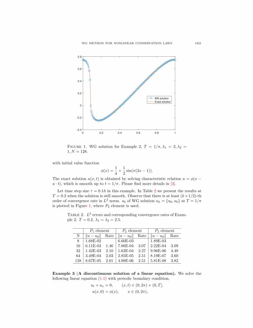
Figure 1. WG solution for Example 2, T = 1/π, λ1 = 2, λ2 =1, N = 128.
with initial value function
φ(x) =1
4+
1
2sin(π(2x− 1)).
The exact solution u(x, t) is obtained by solving characteristic relation u = φ(x −u · t), which is smooth up to t = 1/π. Please find more details in [4].
Let time step size τ = 0.1h in this example. In Table 2 we present the results atT = 0.2 when the solution is still smooth. Observe that there is at least (k+1/2)-thorder of convergence rate in L2 norm. ub of WG solution uh = u0, ub at T = 1/πis plotted in Figure 1, where P2 element is used.
Table 2. L2 errors and corresponding convergence rates of Exam-ple 2. T = 0.2, λ1 = λ2 = 2.5.
P1 element P2 element P3 elementN ‖u− u0‖ Rate ‖u− u0‖ Rate ‖u− u0‖ Rate8 1.68E-02 6.60E-03 1.89E-0316 6.11E-03 1.46 7.86E-04 3.07 2.22E-04 3.0932 1.42E-03 2.10 1.63E-04 2.27 9.96E-06 4.4864 3.49E-04 2.03 2.85E-05 2.51 8.19E-07 3.60128 8.67E-05 2.01 4.98E-06 2.51 5.81E-08 3.82
Example 3 (A discontinuous solution of a linear equation). We solve thefollowing linear equation (1.1) with periodic boundary condition,
ut + ux = 0, (x, t) ∈ (0, 2π)× (0, T ],
u(x, 0) = φ(x), x ∈ (0, 2π),

1922 XIU YE, SHANGYOU ZHANG AND PENG ZHU
0 1 2 3 4 5 6 7
-0.2
0
0.2
0.4
0.6
0.8
1
1.2
WG(1.2,0.1) solution
(a) WG solution with
(λ1, λ2) = (1.2, 0.1)
0 1 2 3 4 5 6 7
-0.2
0
0.2
0.4
0.6
0.8
1
1.2
DG solution
(b) DG solution
Figure 2. The P1 WG solution and DG solution for Example 3,T = 2π,N = 512.
with initial value function
φ(x) =
1, π/2 < x ≤ 3π/2,
0, elsewhere.
The exact solution is u(x, t) = φ(x− t).
In this problem the exact solution is non-smooth. It aims to show our WGmethod is also stable and efficient to the problems with non-smooth solutions. Lettime step size τ = 0.1h in this example. The errors and the order of convergence arereported in Table 3. Observe that the method is stable. The WG solution using P1
element with (λ1, λ2) = (1.2, 0.1) and the DG solution with P1 element are plottedin Figure 2 (a) and (b) respectively.
Table 3. L2 errors and corresponding convergence rates of Exam-ple 3. T = 2π, λ1 = 2, λ2 = 1.
P1 element P2 elementN ‖u− u0‖ Rate ‖u− u0‖ Rate8 5.93E-01 4.23E-0116 5.01E-01 0.24 3.25E-01 0.3832 3.93E-01 0.35 2.52E-01 0.3764 3.26E-01 0.27 1.98E-01 0.35128 2.72E-01 0.26 1.58E-01 0.33256 2.26E-01 0.27 1.27E-01 0.32512 1.89E-01 0.26 1.03E-01 0.30
6. Conclusion. A weak Galerkin finite element method is proposed for nonlinearconservation laws. This method provides a class of finite element schemes by tun-ing the built-in parameters including purely upwind scheme. This makes the WGmethod highly flexible. Compared with the DG method [11], the present methodcan be applied for solving nonlinear conservation laws. Error estimations are given.The convenience of the proposed method is validated by the numerical examples.
WG METHOD FOR NONLINEAR CONSERVATION LAWS 1923
REFERENCES
[1] B. Cockburn and C.-W. Shu, TVB Runge-Kutta local projection discontinuous Galerkin finiteelement method for conservation laws. II. General framework, Math. Comp., 52 (1989), 411–
435.
[2] B. Cockburn and C.-W. Shu, Runge-Kutta discontinuous Galerkin methods for convection-dominated problems, J. Sci. Comput., 16 (2001), 173–261.
[3] S. Gottlieb, C.-W. Shu and E. Tadmor, Strong stability-preserving high-order time discretiza-
tion methods, SIAM Rev., 43 (2001), 89–112.[4] A. Harten, B. Engquist, S. Osher and S. R. Chakravarthy, Uniformly high-order accurate
essentially non-oscillatory schemes. III, J. Comput. Phys., 71 (1987), 231–303.
[5] G. S. Jiang and C.-W. Shu, On cell entropy inequality for discontinuous Galerkin methods,Math. Comp., 62 (1994), 531–538.
[6] M.-Y. Kim, A discontinuous Galerkin method with Lagrange multiplier for hyperbolic con-
servation laws with boundary conditions, Comput. Math. Appl., 70 (2015), 488–506.[7] M.-Y. Kim, High order DG-DGLM method for hyperbolic conservation laws, Comput. Math.
Appl., 75 (2018), 4458–4489.[8] J. Li, X. Ye and S. Zhang, A weak Galerkin least-squares finite element method for div-curl
systems, J. Comput. Phys., 363 (2018), 79–86.
[9] G. Lin, J. Liu, L. Mu and X. Ye, Weak Galerkin finite element methods for Darcy flow:Anisotropy and heterogeneity, J. Comput. Phys., 276 (2014), 422–437.
[10] R. Lin, X. Ye, S. Zhang and P. Zhu, A weak Galerkin finite element method for singularly
perturbed convection-diffusion-reaction problems, SIAM J. Numer. Anal., 56 (2018), 1482–1497.
[11] X. Meng, C.-W. Shu and B. Wu, Optimal error estimates for discontinuous Galerkin methods
based on upwind-biased fluxes for linear hyperbolic equations, Math. Comp., 85 (2016), 1225–1261.
[12] L. Mu, J. Wang and X. Ye, A new weak Galerkin finite element method for the Helmholtz
equation, IMA J. Numer. Anal., 35 (2015), 1228–1255.[13] L. Mu, J. Wang and X. Ye, Weak Galerkin finite element methods for the biharmonic equation
on polytopal meshes, Numer. Methods Partial Differential Equations, 30 (2014), 1003–1029.[14] L. Mu, J. Wang and X. Ye, Weak Galerkin finite element methods on polytopal meshes, Int.
J. Numer. Anal. Model., 12 (2015), 31–53.
[15] L. Mu, J. Wang, X. Ye and S. Zhang, A weak Galerkin finite element method for the Maxwellequations, J. Sci. Comput., 65 (2015), 363–386.
[16] L. Mu, J. Wang, X. Ye and S. Zhao, A new weak Galerkin finite element method for elliptic
interface problems, J. Comput. Phys., 325 (2016), 157–173.[17] S. Shields, J. Li and E. A. Machorro, Weak Galerkin methods for time-dependent Maxwell’s
equations, Comput. Math. Appl., 74 (2017), 2106–2124.
[18] J. Wang and X. Ye, A weak Galerkin finite element method for second-order elliptic problems,J. Comput. Appl. Math., 241 (2013), 103–115.
[19] J. Wang and X. Ye, A weak Galerkin mixed finite element method for second order ellipticproblems, Math. Comp., 83 (2014), 2101–2126.
[20] J. Wang and X. Ye, A weak Galerkin finite element method for the Stokes equations, Adv.Comput. Math., 42 (2016), 155–174.
[21] Q. Zhai, R. Zhang, N. Malluwawadu and S. Hussain, The weak Galerkin method for linearhyperbolic equation, Commun. Comput. Phys., 24 (2018), 152–166.
[22] Q. Zhang and C.-W. Shu, Error estimates to smooth solutions of Runge-Kutta discontinuousGalerkin methods for scalar conservation laws, SIAM J. Numer. Anal., 42 (2004), 641–666.
[23] Q. Zhang and C.-W. Shu, Stability analysis and a priori error estimates of the third orderexplicit Runge-Kutta discontinuous Galerkin method for scalar conservation laws, SIAM J.Numer. Anal., 48 (2010), 1038–1063.
Received April 2020; revised July 2020.
E-mail address: [email protected]
E-mail address: [email protected]
E-mail address: [email protected]