NONLINEAR MODEL REDUCTION USING PETROV-GALERKIN PROJECTION AND DATA

RECONSTRUCTION

Kevin Carlberg and Charbel FarhatStanford University

SIAM Annual Meeting 2010July 13, 2010

Acknowledgements: AFOSR, Toyota, NSF, DoD

! Two main problems arise in nonlinear model reduction:

1. Accuracy/Stability: projection does not always preserve

stability or capture nonlinearities

2. Computational complexity: reduced-order operators are

expensive to assemble, even though they have small

dimension

TECHNICAL ISSUES

! Ahmed body

! Navier-Stokes Simulation

" ! = 20 deg

" V = 60 m/s

" Re = 4.29 x 106

ILLUSTRATION: AHMED BODY ROM

" DES turbulence model

" 146,517 nodes

" 837,894 tetrahedra

! FOM: 879,102 dofs

! POD/Galerkin ROM (typical): 400 dofs (0.046% size of FOM)

AHMED BODY POD/GALERKIN RESULTS

0.25

0.26

0.27

0.28

0.29

0.3

0.31

0.32

0.33

0.34

0.35

0 0.05 0.1 0.15 0.2 0.25

Time (s)

CD

FOM (879,102 dofs)

ROM: Galerkin (400 dofs)

! CPU time (first 0.1 s)

" FOM. 9,292 s

" ROM: Galerkin. 24,984 s

inaccurate/unstable

computationally expensive

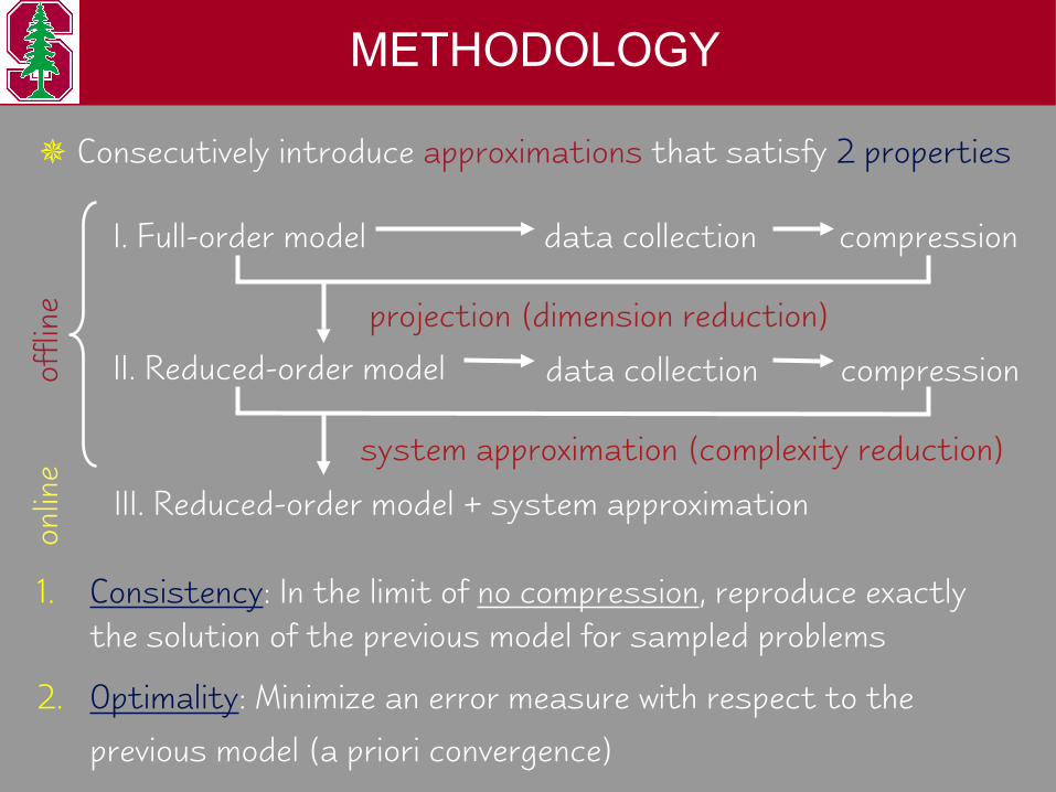
METHODOLOGY

! Consecutively introduce approximations that satisfy 2 properties

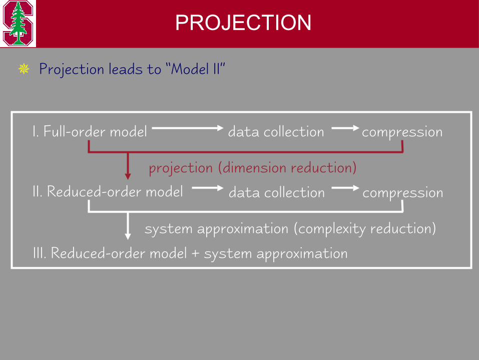
I. Full-order model

II. Reduced-order model

III. Reduced-order model + system approximation

data collection compression

data collection compression

projection (dimension reduction)

system approximation (complexity reduction)

1. Consistency: In the limit of no compression, reproduce exactly the solution of the previous model for sampled problems

2. Optimality: Minimize an error measure with respect to the previous model (a priori convergence)

offli

neon

line

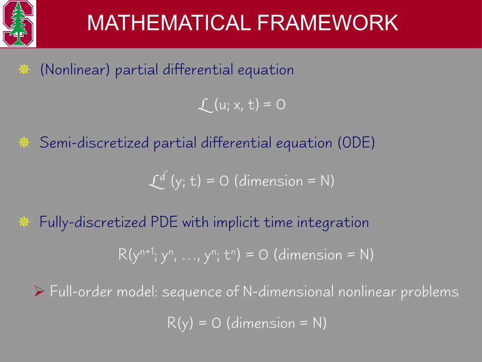
! (Nonlinear) partial differential equation

! Semi-discretized partial differential equation (ODE)

L (u; x, t) = 0

Ld (y; t) = 0 (dimension = N)

! Fully-discretized PDE with implicit time integration

MATHEMATICAL FRAMEWORK

R(yn+1; yn, …, yn; tn) = 0 (dimension = N)

" Full-order model: sequence of N-dimensional nonlinear problems

R(y) = 0 (dimension = N)

PROJECTION

I. Full-order model

II. Reduced-order model

III. Reduced-order model + system approximation

data collection compression

data collection compression

projection (dimension reduction)

system approximation (complexity reduction)

! Projection leads to “Model II”

PETROV-GALERKIN PROJECTION

! To decrease the dimensionality, search for a solution in the

affine subspace: y(0)+range("y) of dimension ny<<N

y#y(0)+"yyr R(y(0)+"yyr)=0

! Enforce residual orthogonal to ny-dimensional subspace range($)

$TR(y(0)+"yyr)=0

! Solve via Newton’s method for k=1,…,K (until converged)

$TJ(k)"yp(k)=-$TR(k)

yr(k+1)=yr

(k)+%(k)p(k)

" R(k)& R(y(0)+"yyr (k)), J(k) & dR/dy(y(0)+"yyr

(k))

! " = [!1 ... !

nx]; "T"=I

COMPRESSION VIA POD

! Proper orthogonal decomposition (POD) method

! Given nx “snapshots” xi, the first k POD vectors satisfy:

Find k ' nx orthonormal vectors minimizing

J(!1 , !2 , …, !k) = ( || xj – ( (xj, !i) !i

||22

j=1

nx

i=1

k

! Properties

! “No compression”: k = nx and range (") = range ([x1 ... xnx])

! Efficient computation by singular value decomposition (SVD)

! Consistency issue: what should the snapshots be?

PROJECTION CONSISTENCY

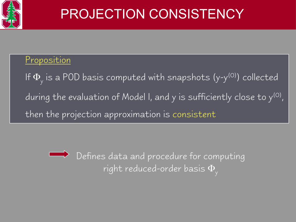
Proposition

If "y is a POD basis computed with snapshots (y-y(0)) collected

during the evaluation of Model I, and y is sufficiently close to y(0),

then the projection approximation is consistent

Defines data and procedure for computing right reduced-order basis "y

! Least-squares Petrov-Galerkin projection

! Equivalent to globally convergent Gauss-Newton method for

! $ is state-dependent, changes each Newton iteration

! Cannot be introduced at ODE level

! Improved accuracy, stability over Galerkin in the general case

PROJECTION OPTIMALITY

! Optimality: would like solution p(k) to satisfy for some norm )

p(k)=arg minp*+ny || "yp-(J(k))-1R(k)||)

! Galerkin: $= "y satisfies (1) with )= J(k) only if J(k) SPD

! Petrov-Galerkin: $= J(k)"y satisfies (1) with )= J(k)TJ(k)

if J(k) nonsingular

(1)

min ||R(y+ "yyr)||2

0.25

0.26

0.27

0.28

0.29

0.3

0.31

0.32

0.33

0.34

0.35

0 0.05 0.1 0.15 0.2 0.25

Time (s)

CD

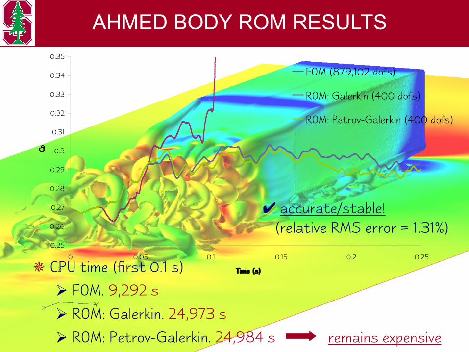
FOM (879,102 dofs)

ROM: Galerkin (400 dofs)

ROM: Petrov-Galerkin (400 dofs)

AHMED BODY ROM RESULTS

! CPU time (first 0.1 s)

" FOM. 9,292 s

" ROM: Galerkin. 24,973 s

" ROM: Petrov-Galerkin. 24,984 s

! accurate/stable! (relative RMS error = 1.31%)

remains expensive

SYSTEM APPROXIMATION

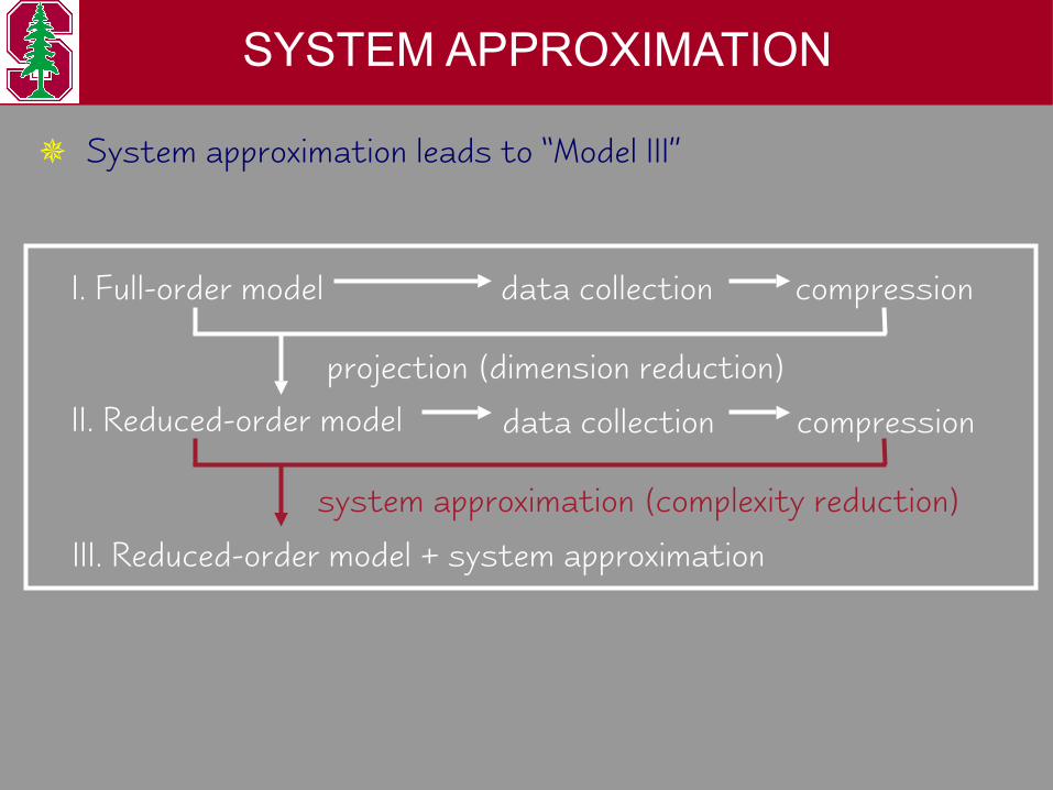
I. Full-order model

II. Reduced-order model

III. Reduced-order model + system approximation

data collection compression

data collection compression

projection (dimension reduction)

system approximation (complexity reduction)

! System approximation leads to “Model III”

SYSTEM APPROXIMATION

! Tensor approximations: R(k) * range("R), J(k) "y * range("J)

! Newton iterations become

J(k) "y # "J Jr(k)

#

R(k) # "R Rr(k)

#invariant

iteration-dependent

[J(k) "y]T[J(k) "y ] p(k) = -[J(k) "y]TR k)

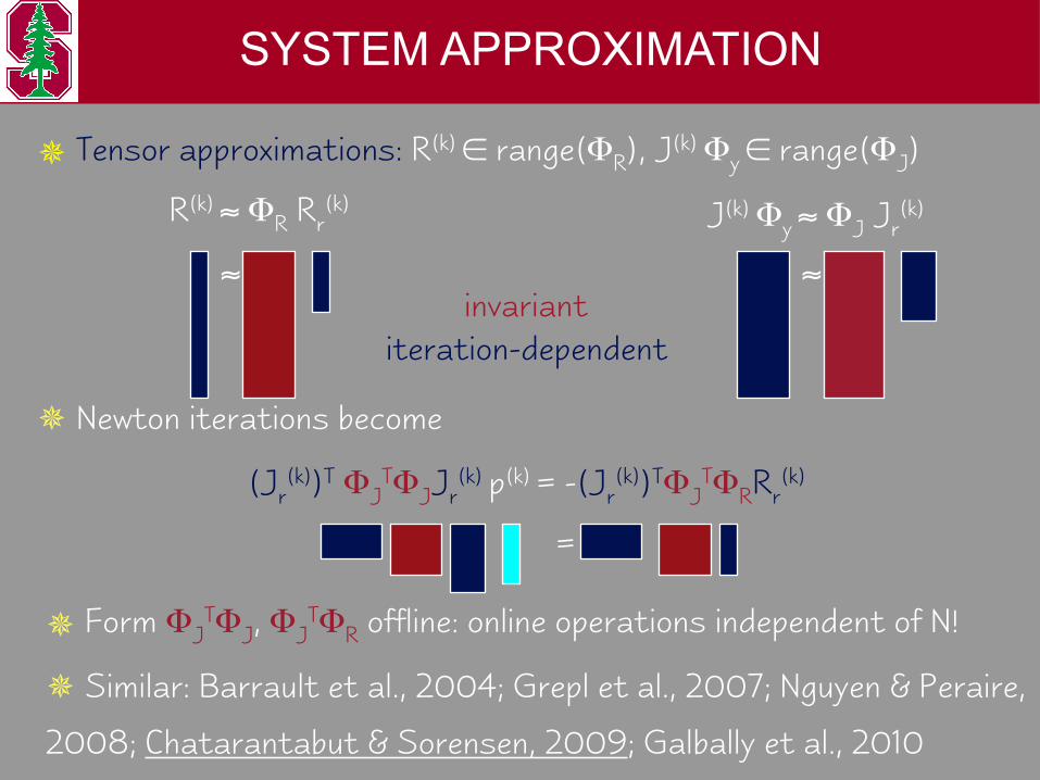
! Form "JT"J, "J

T"R offline: online operations independent of N!

! Similar: Barrault et al., 2004; Grepl et al., 2007; Nguyen & Peraire,

2008; Chatarantabut & Sorensen, 2009; Galbally et al., 2010

SYSTEM APPROXIMATION

! Tensor approximations: R(k) * range("R), J(k) "y * range("J)

! Newton iterations become

J(k) "y # "J Jr(k)

#

R(k) # "R Rr(k)

#invariant

iteration-dependent

(Jr(k))T "J

T"JJr(k)

p(k) = -(Jr(k))T"J

T"RRr(k)

=

SYSTEM APPROXIMATION

! Tensor approximations

J(k) "y # "J Jr(k)

#

R(k) # "R Rr(k)

#

! Property 2: Consistency

" "R, "J computed offline by POD with specific snapshots

! Property 1: Optimality

" Rr(k), Jr

(k) computed online by gappy data reconstruction

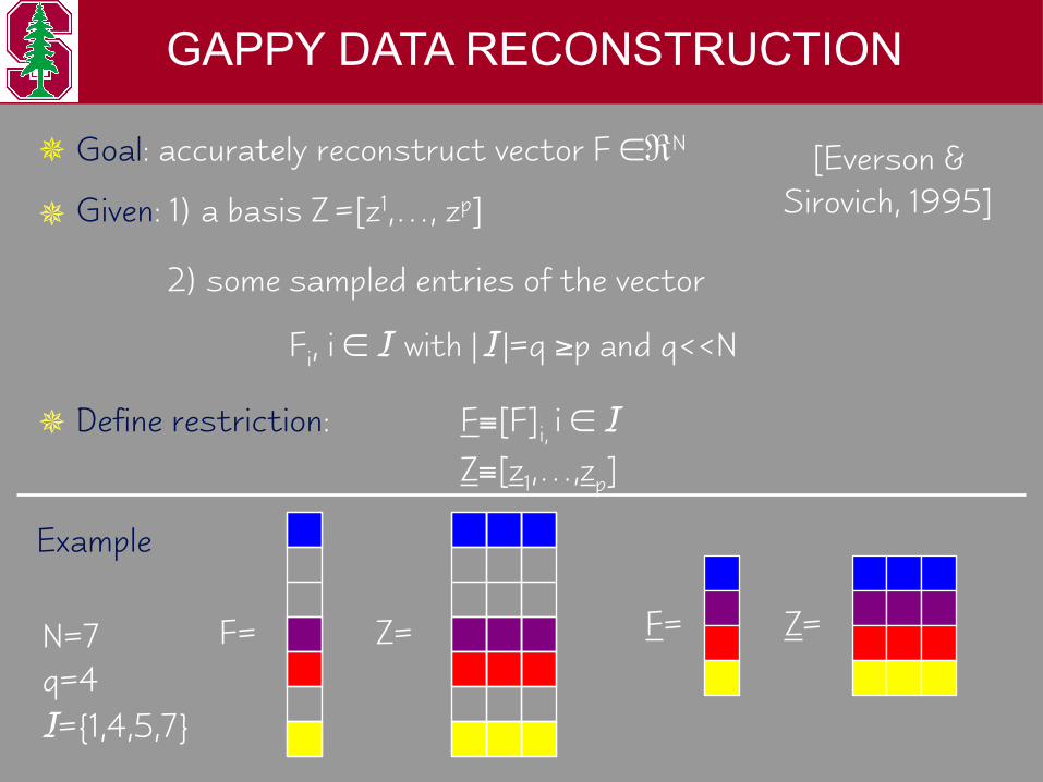
GAPPY DATA RECONSTRUCTION

! Goal: accurately reconstruct vector F *+N

! Given: 1) a basis Z =[z1,…, zp]

2) some sampled entries of the vector

Fi, i * I with | I |=q ,p and q<<N

! Define restriction: F&[F]i, i * I Z&[z1,…,zp]

Example

F= Z= F= Z=N=7q=4I={1,4,5,7}

[Everson & Sirovich, 1995]

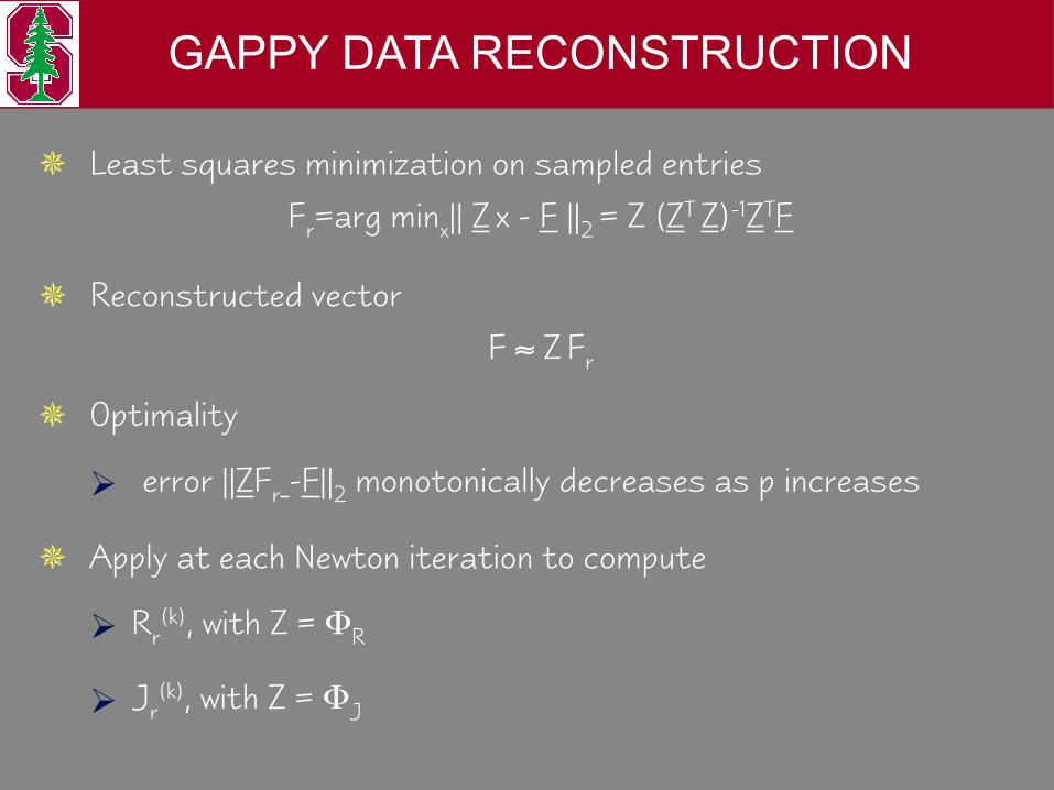
! Least squares minimization on sampled entriesFr=arg minx|| Z x - F ||2 = Z (ZT Z)-1ZTF

! Optimality

" error ||ZFr -F||2 monotonically decreases as p increases

GAPPY DATA RECONSTRUCTION

! Reconstructed vectorF # Z Fr

! Apply at each Newton iteration to compute

" Rr(k), with Z = "R

" Jr(k), with Z = "J

SYSTEM APPROXIMATION CONSISTENCY

Proposition

If "R and "J are POD bases computed with snapshots satisfying

the following conditions:

1. R(k) from the Model II simulation is a snapshot used for "R

2. J(k)"yp(k) from the Model II simulation is a snapshot used for "J

3. Each column of J(k)"y from the Model II simulation is a snapshot used for "J

then the system approximation is consistent

! Leads to hierarchy of snapshot collection procedures characterized

by tradeoffs between consistency and offline cost/storage

SNAPSHOT COLLECTION HIERARCY

" ()I ,()II : snapshot saved during Model I, II

" ()(k): snapshot saved at each Newton iteration

ID 0 1 2 3

Snapshots for y yI-yI(0) yI-yI

(0) yI-yI(0) yI-yI

(0)

Snapshots for R(k) RI(k) RII

(k) RII(k) RII

(k)

Snapshots for J(k)"y RI(k) RII

(k) [J(k)"yp(k)]II [J(k)"y]II

# simulations 1 2 2 2

# snapshots per Newton iteration

1 1 2 1+ ny

consistency conditions satisfied

none 1 1, 2 1, 2, 3

SNAPSHOT COLLECTION HIERARCY

ID 0 1 2 3

Snapshots for y yI-yI(0) yI-yI

(0) yI-yI(0) yI-yI

(0)

Snapshots for R(k) RI(k) RII

(k) RII(k) RII

(k)

Snapshots for J(k)"y RI(k) RII

(k) [J(k)"yp(k)]II [J(k)"y]II

# simulations 1 2 2 2

# snapshots per Newton iteration

1 1 2 1+ ny

consistency conditions satisfied

none 1 1, 2 1, 2, 3

! Procedure 0: most common, yet satisfies no consistency conditions! Procedure 3: consistent, but prohibitive cost for most problems# Procedure 2: similar cost as 1, more consistency conditions

" A = (" T" )-T"JT"J(" T" )-1, B = (" T" )-T"J

T"R( " T" )-1

! The approximated Newton iterations are

! Offline1. Collect snapshots by evaluating

Model I, Model II

2. Compute POD bases "y, "R, "J

3. Determine sample indices I for

gappy reconstruction

4. Compute matrices A, B

PROCEDURE

[J " ]TA [J " ] p(k) = -[J " ]TBR .(k)(k)(k) (k)yyy

! Online (each Newton step)1. Compute r<<n required

state vector entries

2. Compute restricted

quantities by evaluating R(k)

and J(k)"y at q << n indices

3. Solve for p(k)

J J J J J J R R

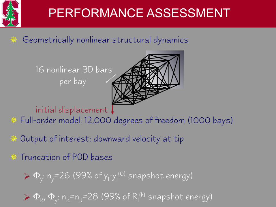
16 nonlinear 3D barsper bay

! Geometrically nonlinear structural dynamics

PERFORMANCE ASSESSMENT

! Full-order model: 12,000 degrees of freedom (1000 bays)

! Output of interest: downward velocity at tip

! Truncation of POD bases

" "y: ny=26 (99% of yI-yI(0) snapshot energy)

" "R, "y: nR=nJ=28 (99% of RI(k) snapshot energy)

initial displacement

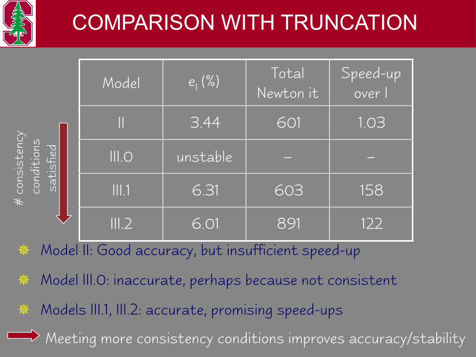
COMPARISON WITH TRUNCATION

Model eI (%) Total Newton it

Speed-up over I

II 3.44 601 1.03

III.0 unstable – –

III.1 6.31 603 158

III.2 6.01 891 122

! Model II: Good accuracy, but insufficient speed-up

! Model III.0: inaccurate, perhaps because not consistent

! Models III.1, III.2: accurate, promising speed-ups

Meeting more consistency conditions improves accuracy/stability

# co

nsis

tenc

y c

ondi

tion

s sa

tisf

ied

LEAST SQUARES V. INTERPOLATION

! Increasing | I | improves accuracy, even stabilizing III.0

Least-squares reconstruction seems better than interpolation

| I |Relative error eI (%) Speed-up over Model

I

III.0 III.1 III.2 III.0 III.1 III.2

28 unstable 6.31 6.01 120 158 122

42 4.95 3.77 3.63 137 152 119

56 4.03 3.50 3.44 129 136 116

! ny=26, nR=nJ=28

interpolation

least squares

! Approximations are consecutively introduced and satisfy

consistency and optimality conditions:

1. Least-squares Petrov-Galerkin projection

2. System approximation

! Numerical experiments indicate

" Petrov-Galerkin projection improves accuracy/stability

" Tensor approximations are accurate/stable when they

satisfy at least some consistency conditions

" Orders of magnitude speed-ups achieved

CONCLUSIONS

QUESTIONS?

K. Carlberg, C. Bou-Mosleh, and C. Farhat, “Efficient Nonlinear Model Reduction via a Least-Squares Petrov-Galerkin Projection and Compressive Tensor Approximations”, International Journal of Numerical Methods in Engineering, submitted.

! For more details, see forthcoming paper: