A Class of Discontinuous Petrov-Galerkin Methods.Part III: Adaptivity

Leszek Demkowicza,∗, Jay Gopalakrishnanb, Antti H. Niemia

aInstitute for Computational Engineering and SciencesThe University of Texas at Austin, Austin, TX 78712, USA

bDepartment of MathematicsUniversity of Florida, FL 32611, USA

Abstract

We continue our theoretical and numerical study on the Discontinuous Petrov-Galerkin method with optimaltest functions in context of 1D and 2D convection-dominated diffusion problems and hp-adaptivity. Witha proper choice of the norm for the test space, we prove robustness (uniform stability with respect to thediffusion parameter) and mesh-independence of the energy norm of the FE error for the 1D problem. Withhp-adaptivity and a proper scaling of the norms for the test functions, we establish new limits for solvingconvection-dominated diffusion problems numerically: ε = 10−11 for 1D and ε = 10−7 for 2D problems. Theadaptive process is fully automatic and starts with a mesh consisting of few elements only.

Keywords: convection-dominated diffusion, hp-adaptivity, Discontinuous Petrov-Galerkin

1. Introduction

We begin with a short review of two main concepts behind the Discontinuous Petrov Galerkin (DPG)Method with Optimal Test Functions introduced in [1]: the abstract idea of optimal test functions, andits practical realization within the DPG method. We follow then with a short comparison with stabilizedmethods and a discussion of the main algorithm. We finish by outlining the scope of this contribution.

1.1. Petrov-Galerkin Method with Optimal Test Functions

Variational problem and energy norm. Consider an arbitrary abstract variational problem,u ∈ U

b(u, v) = l(v) ∀v ∈ V(1.1)

Here U, V are two real Hilbert spaces and b(u, v) is a continuous bilinear form on U × V ,

|b(u, v)| ≤M‖u‖U ‖v‖V (1.2)

that satisfies the inf-sup condition

inf‖u‖U=1

sup‖v‖V =1

|b(u, v)| =: γ > 0 (1.3)

∗Corresponding authorEmail addresses: leszek@ices.utexas.edu (Leszek Demkowicz), jayg@ufl.edu (Jay Gopalakrishnan),

ahniemi@ices.utexas.edu (Antti H. Niemi)

Preprint submitted to Elsevier November 7, 2010

A continuous linear functional l ∈ V ′ represents the load. If the null space of the adjoint operator,

V0 := v ∈ V : b(u, v) = 0 ∀u ∈ U (1.4)

is non-trivial, the functional l is assumed to satisfy the compatibility condition:

l(v) = 0 ∀v ∈ V0 (1.5)

By the Banach Closed-Range Theorem (see e.g. [2]), problem (1.1) possesses a unique solution u that dependscontinuously upon the data – functional l. More precisely,

‖u‖U ≤M

γ‖l‖V ′ (1.6)

If we define an alternative energy norm equivalent to the original norm on U ,

‖u‖E := sup‖v‖=1

|b(u, v)| (1.7)

both the continuity and the inf-sup constant become equal to one. Recalling that the Riesz operator,

R : V 3 v → (v, ·) ∈ V ′ (1.8)

is an isometry from V into its dual V ′, we may characterize the energy norm in an equivalent way as

‖u‖E = ‖vu‖V (1.9)

where vu is the solution of the variational problem,vu ∈ V

(vu, δv)V = b(u, δv) ∀δv ∈ V(1.10)

with (·, ·)V denoting the inner product in the test space V .

Optimal test functions. Let Uhp ⊂ U be a finite-dimensional space with a basis ej = ej,hp, j = 1, . . . , N =Nhp. For each basis trial function ej , we introduce a corresponding optimal test (basis) function ej ∈ V thatrealizes the supremum,

|b(ej , ej)| = sup‖v‖V =1

|b(ej , v)| (1.11)

i.e. solves the variational problem, ej ∈ V

(ej , δv)V = b(ej , δv) ∀δv ∈ V(1.12)

The test space is now defined as the span of the optimal test functions, Vhp := spanej , j = 1, . . . , N ⊂ V .The Petrov-Galerkin discretization of the problem (1.1) with the optimal test functions takes the form:

uhp ∈ Uhp

b(uhp, vhp) = l(vhp) ∀vhp ∈ Vhp(1.13)

It follows from the construction of the optimal test functions that the discrete inf-sup constant

inf‖uhp‖E=1

sup‖vhp‖=1

|b(uhp, vhp)| (1.14)

2

is also equal to one. Consequently, Babuska’s Theorem [3] implies that

‖u− uhp‖E ≤ infwhp∈Uhp

‖u− whp‖E (1.15)

i.e., the method delivers the best approximation error in the energy norm.The construction of optimal test functions implies also that the global stiffness matrix is symmetric and

positive-definite. Indeed,b(ei, ej) = (ei, ej)V = (ej , ei)V = b(ej , ei) (1.16)

Once the approximate solution has been obtained, the energy norm of the FE error ehp := u − uhp isdetermined by solving again the variational problem

vehp ∈ V

(vehp , δv)V = b(u− uhp, δv) = l(δv)− b(uhp, δv) ∀δv ∈ V(1.17)

We shall call the solution vehp to the problem (1.17) as the the error representation function since we have

‖ehp‖E = ‖vehp‖V (1.18)

Notice that the energy norm of the error can be computed (approximately, see below) without knowledge ofthe exact solution. Indeed, the energy norm of the error is nothing else than a properly defined norm of theresidual.

Approximate optimal test functions. In practice, the optimal test functions ej and the error representationfunction vehp are computed approximately using a sufficiently large “enriched” subspace Vhp ⊂ V . Theoptimal test space Vhp is then a subspace of the enriched test space Vhp. For instance, if elements of orderp are used, the enriched test space may involve polynomials of order p+ ∆p. The approximate optimal testspace forms a proper subspace of the enriched space and it should not be confused with the enriched spaceitself, though.

1.2. Discontinuous Petrov Galerkin Method

For conforming discretizations, approximate solution of the variational problem (1.12),ej ∈ Vhp

(ej , δv)V = b(ej , δv) ∀δv ∈ Vhp(1.19)

leads to a global system of equations and, consequently, the whole discussed concept has little practical value.The situation changes, if the above methodology is applied in context of the Discontinuous Petrov Galerkin(DPG) method introduced by Bottasso, Micheletti, Sacco and Causin [4, 5, 6, 7]. The starting point ofthe method is a system of first-order differential equations. The equations are multiplied by test functions,integrated over the domain, and then integrated by parts. Contrary to classical variational formulationswhere some of the equations are relaxed and some others are enforced in a strong form, in the DPG methodall equations are considered in a weak sense. Formulations like this are sometimes termed as ultra-weakvariational formulations.

The key point of the DPG method of Bottasso et al. is anyway the treatment of the boundary flux termsresulting from integration by parts as independent unknowns. This is in contrast to most of the discontinuousGalerkin formulations found in the literature where the boundary terms are related to the field variablessupported over the elements using the concept of numerical flux. The departure from the classical pathmeans that the test and trial functions cannot be chosen within the same spaces so that we are indeed led toa Petrov-Galerkin formulation. The approach is rather transparent since the characteristics of the resultingmethod are dictated mainly by the choice of the finite element spaces for the test and trial functions withoutbeing affected by the specific expressions of the numerical fluxes. In the works of Bottasso and co-workers

3

the FE spaces are chosen explicitly so as to obtain methods with desired optimality properties. However, inthe first two papers of the present series [8, 1], we have taken few steps further by demonstrating how theframework can actually be utilized to compute the optimal test functions once a proper trial space has beenchosen. The optimal test functions turn out to be non-polynomials generally, but they can be approximatedin a computationally efficient manner by using higher order polynomial spaces element-wise.

Inversion of the Riesz operator in context of the DPG method and discontinuous test functions, is doneon the element level by solving problem (1.12) (for the optimal test functions) and problem (1.17)(for theerror representation function). In 2D, this involves solving a variational problem set in H(div,K)×H1(K).In practice, we can solve those problems only approximately by discretizing space H(div,K) × H1(K).The simplest practical solution was to solve the problems using the p-method. With element trial shapefunctions being polynomials of order p, we solve for the approximate optimal test functions in the ”enriched”space Pp+∆p. The minimum value for ∆p is such that the dimension of the enriched space is greater orequal to the dimension of the trial space (for field variables and boundary fluxes combined). Otherwise,the ultimate element stiffness matrix would be singular. Notice that the discretization of the local (self-adjoint and coercive) problems is done using the standard Bubnov-Galerkin method. Standard estimates forthe p-method indicate that with the ∆p → ∞, the approximate optimal test functions (approximate errorrepresentation function) will converge to the exact test functions (error representation function). The p-enrichment was the easiest approach to code. Alternatively, we could use an element subgrid discretization,i.e. an h- or hp-refined element. In principle, we could resolve the optimal test functions even with acontrolled accuracy, using adaptive methods. The optimal test functions are thus elements of the enrichedspace and so is the space of element (approximate) optimal test functions. With the dimension of theenriched space exceeding the dimension of the trial space, the element test space is only a proper subspaceof the enriched space.

The square of the global error given by (1.18) is equal to the sum of the corresponding element contri-butions,

‖ehp‖2E = ‖vehp‖2V =∑K

‖vehp‖2V (K)︸ ︷︷ ︸eK

(1.20)

where the element error representation function vehp is computed by solving a local counterpart of (1.17)using the element enriched space. The individual element contributions eK serve as element error indicatorsand form the basis for adaptive mesh refinement.

Comparison with DG and other Stabilized Methods

We refer to [1, 8, 9] for a partial review of related DG literature. The DG methods are based on theconcept of numerical flux of Peter Lax whose definition requires typically stronger regularity assumptionson the solution than implied by the energy setting, see e.g. the original contributions of Cockburn andShu [10, 11]. For instance, use of traces for the standard DG method for the convection problem is illegalat the continuous level - the L2 functions do not admit traces (see the discussion in [8]). The numericalflux technique can thus be viewed as means of stabilization coming from the boundary of the element(typical DG methods use Bubnov-Galerkin discretization) and in this sense the DG methods fall into awider class of stabilized FE methods. The breakthrough concept of stabilized FE methods which startedwith the Streamline-Diffusion Petrov Galerkin (SUPG) method of Hughes and Brooks [12], has been at theforefront of FE research in CFD for the last three decades. In particular, in the case of “bubble methods”,stabilization comes from introducing and condensing out additional bubble shape functions (i.e. functionsvanishing on the element boundary) [13, 14]. You might say, that the stabilization comes from the elementinterior. Remarkably, the bubble techniques may lead to the same discrete equations as the SUPG method[15]. Except for DPG methods (see [16, 17, 18], majority of stabilized methods is restricted to low orderelements. The common property of all stabilized methods is a proper modification of the bilinear and linearform at the discrete level without violating the consistency. Contrary to those methods, the stability of theDPG method with optimal test functions comes only from the optimal testing (computed on the fly). Nomodifications are made to the original bilinear and linear forms. The DPG method is directly linked with

4

the concept of generalized least squares method see e.g. [19]. If we write the original variational problem inthe operator form,

Bu = l, B : U → V ′, < Bu, v >= b(u, v) (1.21)

precondition it with the inverse of the Riesz operator in test space V ,

R−1V Bu = R−1

V l, R−1V B : U → V (1.22)

and apply the least squares in the test space V ,

‖R−1V Buhp −R−1

V l‖2V → min (1.23)

we obtain exactly the DPG method.

Implementation of the DPG method. Implementation of DPG with optimal testing requires minimal changeswhen compared with standard hybrid methods. All numerical experiments presented in this paper weredone with a standard frontal solver that requires returning for each element local-to-global connectivities forelement degrees-of-freedom (d.o.f.), and the corresponding element matrices. Similarly to Raviart-Thomaselements, the DPG method involves local (interior) d.o.f. related to “field variables” and d.o.f. correspondingto the DPG fluxes that live on element edges and are shared by adjacent elements. The corresponding trialshape functions are only globally L2-conforming, so no global continuity need to be enforced. The essentialdifference comes in the element routine. Using the enriched space polynomials, we set up the auxiliaryvariational problem (1.12) and solve it approximately using the standard Bubnov-Galerkin method andthe enriched space. One can think of a miniature spectral FE problem defined on one element. Note thefollowing simple observations.

• The local problem (1.12) involves multiple right-hand sides. We perform the LU decomposition of thestiffness matrix once and follow with multiple back substitutions.

• Once the optimal shape functions have been determined, the actual problem element stiffness matrixis computed utilizing relation (1.16). We integrate for the load vector, however, using the standardprocedure.

• In the case of uniform meshes, both in terms of geometry, material properties and polynomial order,the element optimal test functions can be precomputed.

Computation of error representation function and the corresponding element contribution to the energyerror is done using the same algorithm except for a different load to the local problem, comp. (1.17). Noticea similarity with the implicit a-posteriori error estimation techniques using equilibriated residuals [20]. Themain difference lies in the fact that, in the case of the DPG method, there is no need to equlibriate theelement residuals.

Scope of this paper. The present work is a continuation of [1] and focuses on convection-dominated diffusionproblems. In Section 2, we present a refined stability analysis for the 1D problem and show how a properchoice of the norm for the test functions leads to a robust method, i.e. a method uniformly stable with respectto the diffusion parameter ε. We also prove a fundamental property of the error representation function –global continuity. The main focus of the paper though is automatic adaptivity. Section 3 presents numericalresults for the 1D problem, and in Section 4 we share our 2D experience. With a clever choice of norms forthe test functions we achieve not only the robustness but have also been able to push the existing limitsfor solving convection-dominated diffusion problems using high-order finite elements with double precisionarithmetic. Concerning the lowest possible value of the diffusion parameter, the new “records” are ε = 10−11

for 1D, and ε = 10−7 for 2D problems. Most importantly, the whole mesh optimization process is completelyautomatic and starts with an initial mesh consisting of few elements only.

5

2. Convection-Dominated Diffusion in 1D

In this section, we continue our study on a 1D convection-dominated diffusion model problem initiatedin [1]. We demonstrate that, with a proper choice of the norm for the test functions, we may obtain arobust DPG method, i.e. a method whose stability properties are uniform in the diffusion parameter ε. Moreprecisely, we show that the standard L2-norm of the velocity u and the stress σ = εu′ is bounded by theDPG energy norm times an ε-independent constant of order one.

In general, the expression of the DPG energy norm is mesh dependent. If we h-refine the mesh, theexpression changes and there is no guarantee that the error in this norm would decrease. However, if wework with the standard (possibly weighted) H1-norm for the test functions,

‖v‖2K =

∫K

(|v′|2 + |v|2)α(x) dx (2.24)

the corresponding energy norm of the FE error turns out to be mesh-independent in the following sense: Wewill show that the DPG energy norm of the FE error for an arbitrary hp mesh coincides with the spectral(one element) DPG energy norm of the error.

1D model problem. Given a right-hand side f(x), x ∈ (0, 1) and inflow data u0, we consider the problem:u(0) = u0, u(1) = 0

1

εσ − u′ = 0

−σ′ + u′ = f

(2.25)

Introducing an arbitrary partition,

0 = x0 < x1 < . . . < xk−1 < xk < . . . < xN = 1 (2.26)

we formulate the DPG method as follows. The unknowns include field variables σk, uk defined over element(xk−1, xk) and approximated with (equal) order polynomials Pp(xk−1, xk) and fluxes σ(xk), u(xk), k =0, . . . , N . Fluxes u(0) = u0, u(1) = 0 are known from the boundary conditions. For each element K =(xk−1, xk), we have test functions (τ, v) = (τk, vk). Polynomial order p may vary from element to element.Consistently with the L2-energy setting for σ, u, the discretization is globally discontinuous.

For each k = 1, . . . , N , we satisfy the following variational equations,1

ε

∫ xk

xk−1

σkτ +

∫ xk

xk−1

ukτ′ −(uτ)|xkxk−1

= 0∫ xk

xk−1

σkv′ −(σv)|xkxk−1

−∫ xk

xk−1

ukv′ +(uv)|xkxk−1

=

∫ xk

xk−1

fv(2.27)

for every optimal test function τ, v. Again, for k = 1, u(0) = u0 is known and is moved to the right-handside. Similarly, u(1) = 0 in the last equation for k = N .

Norm for the test functions. The norm for the test functions is defined element-wise:

‖(τ ,v)‖ =

(N∑k=1

‖τk‖2k + ‖vk‖2k

) 12

(2.28)

We will work with two choices for the element norms,

6

• A weighted H1-norm,

‖τk‖2k =

∫ xk

xk−1

α(|τ ′k|2 + |τk|2) dx

‖vk‖2k =

∫ xk

xk−1

α(|v′k|2 + |vk)|2) dx(2.29)

• A mesh-dependent norm,

‖τk‖2k =

∫ xk

xk−1

α|τ ′k|2 + βk|τk(xk)|2 dx

‖vk‖2k =

∫ xk

xk−1

α|v′k|2 + βk|vk(xk)|2 dx(2.30)

Notice that, for a globally continuous function, the norm corresponding to element norm (2.29) reduces to amesh-independent global (spectral) norm, whereas in the second case, it does not. Weights α = α(x), βk, k =1, . . . , N are to be selected.

Global Continuity of the Error Representation Function

We start with a notation. Let U = (σ,u, σ, u) denote the exact solution,

σ := (σ1, . . . , σN )u := (u1, . . . , uN )σ := (σ(x0), . . . , σ(xN ))u := (u(x1), . . . , u(xN−1))

(2.31)

and Uhp the corresponding approximate counterpart. Consider two neighboring elements (xk−1, xk), (xk, xk+1).Let (τσk , vσk) be the optimal, vector-valued test function corresponding to flux σk, spanned over the twoelements. We have the standard orthogonality condition for the error function Ehp := U − Uhp,

b(U − Uhp, (τσk , vσk)) = bk(U − Uhp, (τσk , vσk)) + bk+1(U − Uhp, (τσk , vσk)) = 0 (2.32)

Here bk denotes the k-th element contribution to the bilinear form defined by (2.27). Let (φk, ψk) be nowthe error representation function for the k-th element,

(φk, ψk) ∈ V ((xk−1, xk))

((φk, ψk), (δφ, δψ))k = bk(Ehp, (δφ, δψ)), ∀(δφ, δψ) ∈ V ((xk−1, xk))(2.33)

Here (·, ·)k denotes the inner product corresponding to element norm ‖ ·‖k, and V ((xk−1, xk)) is the elementtest space. For the exact optimal test functions V ((xk−1, xk)) = H1((xk−1, xk)), for the approximate testfunctions, V ((xk−1, xk)) = Pp+∆p((xk−1, xk)) where p is the element order of approximation that varieswith element, and ∆p is a global increment in p defining the enriched space. We have,

((φk, ψk), (τσk , vσk))k + ((φk+1, ψk+1), (τσk , vσk))k+1 = b(U − Uhp, (τσk , vσk)) = 0 (2.34)

On the other side, the definition of optimal test functions implies that

((τσk , vσk), (δφ, δψ))k = −δψ(xk), ∀(δφ, δψ) ∈ V ((xk−1, xk)) (2.35)

and((τσk , vσk), (δφ, δψ))k+1 = δψ(xk), ∀(δφ, δψ) ∈ V ((xk, xk+1)) (2.36)

Selecting the error representation functions (φk, ψk) and (φk+1, ψk+1) for (δφ, δψ) above, and summing upthe two equations, we get

−ψk(xk) + ψk+1(xk) = 0 (2.37)

7

In a similar way, we use the optimal test function corresponding to flux u(xk) to demonstrate that φk(xk)−φk+1(xk) = 0 as well. Application of the same argument to the fluxes at the endpoints x0 = 0 and xN = 1shows that the corresponding error representation function vanishes there. The discussed result is verygeneral and it holds for any choice of inner products for the test functions and other systems of differentialequations as well.

Continuity of the error representation function has an important implication. Solution of the globalproblem

(φ, ψ) ∈ V ((0, 1))

((φ, ψ), (δφ, δψ)) = b(Ehp, (δφ, δψ)), ∀(δφ, δψ) ∈ V ((0, 1))(2.38)

leads to a error representation function (φ, ψ) where φ, ψ coincide with the unions of the element errorrepresentation functions φk, ψk. In order to see it, consider globally continuous test functions (δτ, δv) andsum up the local problems corresponding to element error representation functions (τk, vk) to obtain

(τ, δτ) =

N∑k=1

(τk, δτ)k =

N∑k=1

1

ε

∫ xk

xk−1

σkδτ +

∫ xk

xk−1

ukδτ′ − [uδτ ]|xkxk−1

=

1

ε

∫ 1

0

σδτ +

∫ 1

0

uδτ ′

(v, δv) =

N∑k=1

(vk, δv)k =

N∑k=1

∫ xk

xk−1

σkδv′ − [σδv]|xkxk−1

−∫ xk

xk−1

ukδv′ − [uδv]|xkxk−1

=

∫ 1

0

σδv′ −∫ 1

0

uδv′

(2.39)

where σ and u represent unions of σk and uk, respectively. In other words, continuous test functions δτ, δv“do not see” the jump terms corresponding to inter-element fluxes. This has an important consequence incase of (2.29) because then, for continuous functions, the global norm (2.28) obtained by summing up theelement norms coincides with the spectral, one-element norm. Consequently, the DPG energy norm of theFE error also coincides with the spectral energy norm. In general, convergence analysis of discontinuousGalerkin methods is based on mesh-dependent norms and, usually, one has to work rather hard to boundthose from below by standard L2-type norms. For the DPG method with optimal test functions, at least inthe 1D case, the analysis reduces to the spectral case only.

Another important consequence is the behavior of the energy norm of the error during refinements. Asthe DPG method with optimal test functions delivers the best approximation in the energy norm, the errorcannot increase for a p-refined mesh. The discussed result implies that this holds true for h-refinements aswell. Continuity of the error representation function and non-increase of the error are, of course, true onlyunder the assumption of exact integration and arithmetic and, for this reason, the lack of either in practicalcomputation is a great indicator of round off error effects.

Spectral Stability Analysis

We begin with a slight generalization of the stability analysis for the spectral case presented in [1] andnorm (2.30) with β = 1. In particular, we will find a suitable choice for weight α to guarantee the robustnessof the method.

Following the reasoning in [1] (see also Appendix A), we derive the explicit formula for the energy norm,

‖(σ, u, σ(0), σ(1))‖2E =

‖1

ε

∫ x

0

σ(s) ds− u(x)‖21/α + ‖ − σ(x) + u(x) + σ(0)‖21/α + |1ε

∫ 1

0

σ(s) ds|2 + | − σ(1) + σ(0)|2(2.40)

where ‖ · ‖1/α denotes the weighted L2-norm with weight 1/α. The use of norm (2.30) is essential inestablishing the explicit formula for the energy norm.

8

Formula (2.40) and triangle inequality lead to:

‖1

ε

∫ x

0

σ − σ(x) + σ(0)‖21/α ≤ ‖(σ, u, σ(0), σ(1))‖2E

|1ε

∫ 1

0

σ|2 ≤ ‖(σ, u, σ(0), σ(1))‖2E(2.41)

Denoting,1

ε

∫ x

0

σ − σ(x) + σ(0) =: g(x),1

ε

∫ 1

0

σ =: A

we solve for σ to obtain,

σ(x) = σ(0)exε − g(x)− 1

ε

∫ x

0

ex−sε g(s) ds (2.42)

Integrating both sides over (0, 1) and dividing by ε, we get

A = σ(0)(e1ε − 1)− 1

ε

∫ 1

0

e1−sε g(s) ds (2.43)

Solving for σ(0), we obtain,

σ(0) = Ae−

1ε

1− e− 1ε

+1

ε(1− e− 1ε )

∫ 1

0

e−sε g(s) ds (2.44)

Now comes the main point. If we control function g only in the L2-norm, then the stability constant reflectingdependence σ(0) upon g is of order ε−

12 , i.e. the stability is not uniform with respect to ε (the method is not

robust). If, however, function g is controlled in a weighted norm, we have a chance for robustness. Indeed,choosing for instance

α(x) =

ε2 0 < s < − ε

2 ln( ε2 )

1 − ε2 ln( ε2 ) < s < 1

(2.45)

we have (see Appendix B),

|∫ 1

0

e−sε g(s) ds| ≤

√2ε‖g‖1/α (2.46)

which leads to the final estimate,

|σ(0)| ≤ e−1ε

1− e− 1ε

A+1

(1− e− 1ε )‖g‖1/α (2.47)

where ‖ · ‖1/α is the weighted L2-norm with weight 1/α.

L2-stability result for σ. Substituting expression for σ(0) into (2.42), we get the final formula for the stress,

σ(x) =A

1− e− 1ε

ex−1ε +

1

ε(1− e− 1ε )

∫ 1

0

ex−sε g(s) ds− g(x)− 1

ε

∫ x

0

ex−sε g(s) ds

=A

1− e− 1ε

ex−1ε +

e−1ε

ε(1− e− 1ε )

∫ x

0

ex−sε g(s) ds− g(x) +

1

ε(1− e− 1ε )

∫ 1

x

ex−sε g(s) ds

(2.48)

The L2-norm of σ is bounded in terms of the constant A and the L2-norm of g. We have shown in [1] thatthe corresponding constants are independent of ε, i.e. the method is robust in σ without using the weights.Since the standard L2-norm of g is controlled by the weighted norm ‖ ·‖1/α, we also can claim correspondingestimate using the weighted norm for g,

‖σ‖L2 ≤ C(|A|+ ‖g‖1/α) (2.49)

where the constant C is independent of ε.

9

L2-stability result for u. Once we can control σ(0) and σ in L2-norm, formula for the energy norm impliesthat we also control u in L2-norm. Indeed,

‖ − σ + u+ σ(0)‖2 ≤ ‖ − σ + u+ σ(0)‖21/α ≤ ‖(σ, u, σ(0), σ(1))‖2E (2.50)

and the triangle inequality imply that

‖u‖2 ≤ 2(‖σ‖2 + |σ(0)|2 + ‖ − σ + u+ σ(0)‖2) ≤ C‖(σ, u, σ(0), σ(1))‖2E (2.51)

where constant C is independent of ε.

FE Stability Result

Equivalence of the norms (2.29) and (2.30) on the spectral level implies that the proved spectral stabilityresults hold also for the norm (2.29). The global continuity of the error representation function associatedwith this norm implies that the discussed stability relations between the L2 and energy norms are valid onan arbitrary mesh for the FE error function Ehp = U − Uhp.

It is possible to establish a slightly stronger algebraic result by using the norm (2.30) for the test functions.With an appropriate choice of the parameters βk, the L2 norms of both σ and u can be bounded by theenergy norm of U times an ε-independent constant for any function U for which the energy is finite. Theproof involves the use of “telescoping sums” and can be found in Appendix A.

3. 1D Numerical Experiments

In this section we present numerical results for the 1D convection-dominated diffusion model problemstudied in the previous section. All experiments are reported for the data f = 0 and u0 = 1. Thecorresponding solution develops a boundary layer at x = 1:

σ(x) = − 1

1− e− 1ε

ex−1ε , u(x) =

1

1− e− 1ε

(1− e

x−1ε

)(3.52)

All reported numerical experiments start with a mesh of four elements of order p = 0 (piecewise constants).We have used the norm (2.29) for computing the optimal test functions and the error representation functions.In place of the weight α(x) used in the proof of robustness, we have used a simpler choice,

α(x) =

0.1 x ∈ (0, 1

4 )

1.0 x ∈ ( 14 , 1)

(3.53)

The increment ∆p used to define the enriched space was set to ∆p = 4, and the maximum order was setto pmax = 4. These choices are related to an attempt to determine the minimum diffusion parameter ε forwhich we can solve the problem numerically using double precision arithmetic.

We have used a so called “poor man greedy hp algorithm” summarized below to guide the mesh refine-ments.

10

Set δ = 0.5do while δ > 0.1solve the problem on the current mesh

for each element K in the mesh

compute element error contribution eKend of loop through elements

for each element K in the mesh

if eK > δ2 maxK eK then

if new h ≥ ε then

h-refine the element

elseif new p ≤ pmax then

p-refine the element

endif

endif

end of loop through elements

if (new Ndof = old Ndof) reset δ = δ/2end of loop through mesh refinements

The strategy reflects our old experiments with boundary layers [21], and the rigorous approximability resultsof Schwab and Suri [22] and Melenk [23] on optimal hp discretizations of boundary layers: we proceed withh-refinements until the diffusion scale ε is reached and then continue with p-refinements.

We start with an easy case of ε = 10−3. Fig. 1 presents the corresponding convergence history on a log-logscale, the energy norm of the error vs. the number of degrees-of-freedom (d.o.f.). As predicted by the theory,the error goes monotonically down. The curve displays three different regions. The first one corresponds to aseries of h-refinements “localizing” the boundary layer and is characterized with relatively slow convergence.The second region, characterized with a rapid convergence, corresponds to the p-refinements in the boundarylayer and illustrates the power of p-refinements on a properly refined mesh. Finally, the last part correspondsto the last few refinements when the mesh restrictions in terms of both minimum element size and maximumpolynomial order, become active. Fig. 2 presents a 10× zoom on the boundary layer revealing the “optimal”hp mesh obtained using our algorithm and perfect resolution of the boundary layer (eye ball norm). Finally,Fig. 3 displays the corresponding error representation function φ. The function is continuous consistentlywith the theory.

We continue now with a more challenging case with ε = 10−6. Fig. 4 presents the convergence historyshowing that the error goes monotonically down until the last few refinements where it begins to oscillate.Fig. 5 presents a 105× zoom on the boundary layer revealing the optimal hp mesh and (still) a perfectresolution of the boundary layer. So far, everything looks OK. If we look however at Fig. 6 showing theerror representation function φ, we see that, contrary to the theory, the function is no longer globallycontinuous. For ε = 10−7 the method falls apart and the code reports zero pivots in solving local problemsfor optimal test functions. The loss of continuity of the error representation functions (the same behavioris observed for function ψ) is visible, starting already with ε = 10−4. For elements resolving the boundarylayer, element size h = ε. The ratio of the stiffness and mass terms in formula (2.29) is of order p2/h2 and,for h = 10−3, p = 4, is of order 107, which corresponds to half of the 14–15 digits available in double precisionarithmetic. With h = 10−4, the overlap is minimized to 5 digits and we begin to observe the effects of roundoff errors 1. Apparently, the problems are not limited only to the solution of the element, local problems forthe optimal test functions. To investigate the issue, we have employed for local shape functions (a basis forthe enriched space used to determine optimal test functions and solve for the error representation functions)

1The situation resembles experience with penalty methods.

11

Figure 1: Diffusion parameter ε = 10−3: convergence history.

Figure 2: Diffusion parameter ε = 10−3: resolution of the boundary layer; exact solution u and numerical solution uhp overlapwith each other.

approximate eigenvectors of the 1D Laplacian (with Neumann boundary conditions),λn ∈ IR, φn ∈ Pp+∆p(0, 1)∫ 1

0

φ′nδφ′ dξ = λn

∫ 1

0

φnδφ dξ, ∀δφ ∈ Pp+∆p(0, 1)(3.54)

12

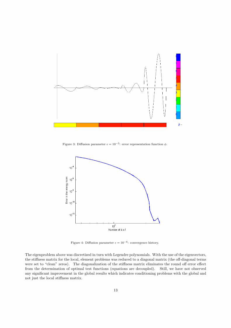
Figure 3: Diffusion parameter ε = 10−3: error representation function φ.

Figure 4: Diffusion parameter ε = 10−6: convergence history.

The eigenproblem above was discretized in turn with Legendre polynomials. With the use of the eigenvectors,the stiffness matrix for the local, element problems was reduced to a diagonal matrix (the off-diagonal termswere set to “clean” zeros). The diagonalization of the stiffness matrix eliminates the round off error effectfrom the determination of optimal test functions (equations are decoupled). Still, we have not observedany significant improvement in the global results which indicates conditioning problems with the global andnot just the local stiffness matrix.

13

Figure 5: Diffusion parameter ε = 10−6: resolution of the boundary layer.

Figure 6: Diffusion parameter ε = 10−6: error representation function φ.

A remedy. A simple idea that came to mind was to work with a rescaled inner product:

(vk, δv)k =

∫ xk

xk−1

(hkv′kδv′ + vkδv)α(x) dx (3.55)

14

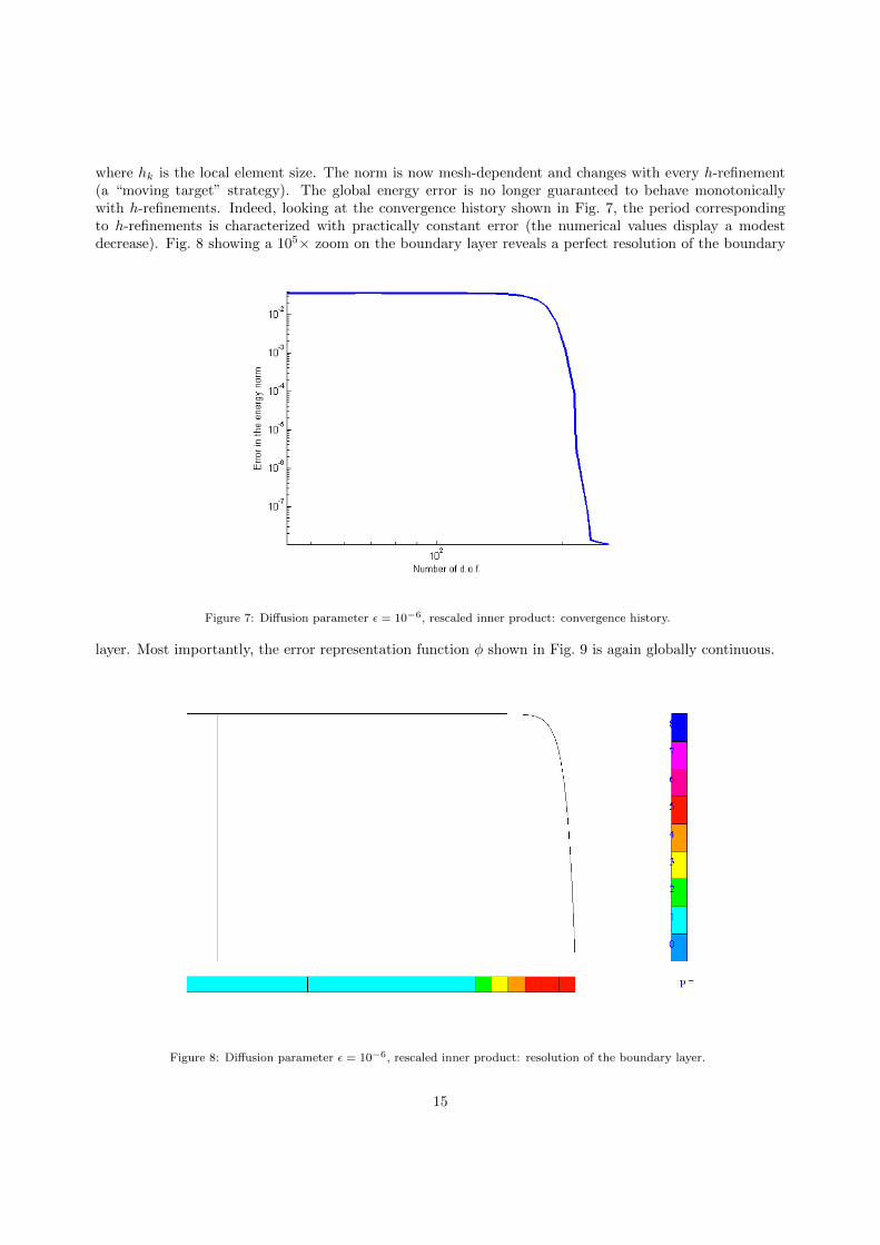
where hk is the local element size. The norm is now mesh-dependent and changes with every h-refinement(a “moving target” strategy). The global energy error is no longer guaranteed to behave monotonicallywith h-refinements. Indeed, looking at the convergence history shown in Fig. 7, the period correspondingto h-refinements is characterized with practically constant error (the numerical values display a modestdecrease). Fig. 8 showing a 105× zoom on the boundary layer reveals a perfect resolution of the boundary

Figure 7: Diffusion parameter ε = 10−6, rescaled inner product: convergence history.

layer. Most importantly, the error representation function φ shown in Fig. 9 is again globally continuous.

Figure 8: Diffusion parameter ε = 10−6, rescaled inner product: resolution of the boundary layer.

15

Figure 9: Diffusion parameter ε = 10−6, rescaled inner product: error representation function φ.

The minimum value of ε, we have been able to solve for with the rescaled inner product, is ε = 10−11.We have tried to increase the power of the element size hk in (3.55) beyond one. It looks like the methoddoes work with an exponent greater than one (e.g. 1.1 − 1.3) but falls apart when the exponent equals 2.As practical range of interest is ε ≥ 10−7, we have been content with the use of (3.55).

Remark 1 All numerical results presented in this and subsequent sections were carried out using ourhp FE codes supporting the whole exact sequence. In other words, the 1D code supports both H1- andL2-conforming elements, whereas the 2D code supports H1-, H(curl)- and L2-conforming elements. Theorders for elements of different conformity type are related. Corresponding to 1D H1-conforming element oforder p is L2-conforming element of order p− 1. The color code in pictures presenting meshes correspondsalways to the H1-conforming elements. This means that the actual order of approximation used for the 1DL2-conforming elements, is one order less. Similarly, the order for quads in 2D drops by one as we movefrom H1 to L2-conforming elements. However, as our 2D code supports only Nedelec triangles of the secondtype, the order for L2-conforming triangles is always p − 2, with p being the order of the correspondingH1-conforming element. For details on exact sequences and hp discretizations, see [24].

4. 2D Numerical Experiments

We consider now the 2D convection-dominated diffusion problem1

εσ −∇u = 0 in Ω

−divσ + div(βu) = f in Ω(4.56)

accompanied with boundary condition for velocity u,

u = u0 on ∂Ω (4.57)

where Ω ⊂ IR2, right-hand side f and boundary data u0 are given, and β is a prescribed advection field.

16

Given an element K, we multiply equations (4.56) with test functions τ , v, integrate over the element,and integrate by parts to arrive at the variational formulation:

1

ε

∫K

στ +

∫K

u divτ −∫∂K

uτn = 0 ∀τ∫K

σ∇v −∫∂K

σnsgn(n)v −∫K

u β · ∇v +

∫∂K

uβnv =

∫K

fv ∀v(4.58)

where the normal stress σn and the velocity u have become independent unknowns on the boundary of theelement. The normal stress is defined using a globally fixed normal ne for element edge e, with functionsgn(n) indicating consistency of global and local, element outward normal unit vectors,

sgn(n) =

1 if n = ne

−1 if n = −ne(4.59)

Energy setting. Presence of the gradient and divergence operators acting on test functions and Cauchy-Schwarz inequality clearly suggest the choice of the space H(div,K) for τ and H1(K) for v as well as thespaces L2(K) and L2(K) for the field unknowns σ and u, respectively. Recall that in 1D the fluxes are justnumbers so their functional setting is rather trivial. In the multi-dimensional setting the fluxes should bein the space dual to the test functions: ∏

K

(H(div,K)×H1(K)) (4.60)

Remark 2 A concrete characterization of the flux spaces was recently given in [9]. The trace un comes

from space H1/2(Γ0h) defined as the space of traces of functions from H1

0 (Ω) to the internal skeleton of themesh:

Γ0h = Γh − ∂Ω where the skeleton Γh =

⋃K

∂K ,

and the flux σn ∈ H1/2(Γh) where H1/2(Γh) denotes the space of traces of functions from H(div,Ω) tothe mesh skeleton. Both spaces are equipped with the minimum energy extension norms. These facts wereunknown to us at the time of writing this paper and the remark was added during the review process.

Discretization. We will compute with both triangular and quadrilateral elements, restricting ourselves to1-irregular meshes only. Each element K supports two field variables: the vector values stress σ and thevelocity u. Each element edge supports two fluxes: the normal stress σn and the velocity u. For triangles,we use the spaces Pp, whereas for quads we use the spaces Q(p,q) = Pp ⊗ Pq with the standard relation

φ(x) := φ(ξ), x = xK(ξ) (4.61)

between the master and physical element shape functions. Here xK stands for the element map transformingthe corresponding master triangle or square into the physical element. The logic of exact sequence and L2-conforming discretizations suggests a slightly different relation between the physical element shape functionsφ(x) and the master element shape functions φ(ξ) [24],

φ(x) :=1

jφ(ξ), x = xK(ξ) (4.62)

where j denotes the jacobian for the element map, j = det(∇xK). However, all presented numerical exampleswill involve affine element only, for which the difference between the two relations reduces to a local scalingwith the constant jacobian only. Element order of approximation p for triangles and (p, q) for quads canvary locally, from element to element.

17

Discretization for fluxes is fixed using a maximum rule. For two neighboring triangles of order p1 andp2, the order for the shared edge is set to

pe = maxp1, p2+ 1 (4.63)

There is no particularly strong reason for raising the order for the edge by one. It is mostly a legacy issuereflecting our initial experience with the DPG method for pure convection problems [8]. In the case ofhanging nodes and an edge with two small neighbors on one side and equal size neighbor on the other, thediscretization for the flux is chosen to be piecewise polynomial with the order set to the maximum of ordersfor all three neighboring elements,

pe = maxp1, p2, p3+ 1 (4.64)

In that sense the maximum rule applies here to both element order and size.We use the same principle for quadrilateral meshes accounting for the directionality of approximation.

This time, again for no deep reason, we chose to set the order of fluxes just to the maximum of the directionalorders for the neighboring elements,

pe = maxq1, q2, q3 (4.65)

Here qi is the order of discretization of the i-th neighbor in the direction of the edge.For each element trial shape function and for each edge trial shape functions, we determine the optimal

test function by solving the local problem,τK ∈ V (K), vK ∈ V (K)

(τK , δτ )H(div) + (vK , δv)H1 = bK((σ, u, σn, u), (δτ , δv)) ∀δτ ∈ V (K), δv ∈ V (K)(4.66)

where V (K), V (K) are the enriched spaces: Pp+∆p for triangular elements, and Pp+∆p ⊗Pq+∆p for quads.At this point we have ignored H(div)-conforming elements and approximated components of τ and δτ withpolynomials of equal order. Despite the piecewise polynomial fluxes for 1-irregular meshes, we have notexperimented yet with piecewise polynomials for the enriched spaces corresponding to a local h-refinementbut intend to do so in future work. The optimal test functions corresponding to the field variables σ, uspan over one element only whereas the optimal test functions corresponding to the fluxes σn, u span overthe elements neighboring the particular edge. Fluxes u on the boundary of the domain are determined byperforming L2-projections of the corresponding boundary data onto the corresponding trial space.

Finally, we start our experiments with weighted inner products for the H(div) and H1 spaces,

(τ , δτ )H(div) =

∫K

divτ divδτ + τ δτw(x) dx

(v, δv)H1 =

∫K

∇v∇δv + v δvw(x) dx(4.67)

The same setting is used to determine the element error representation functions (ψK , φK).All 2D numerical experiments reported in this paper were done for a unit square domain Ω = (0, 1)2,

constant advection vector β, and boundary conditions defined in Fig. 10. The weight w(x) for the innerproducts (4.67) was selected following our 1D experience and is shown in Fig. 11. In 2D the situationis a bit more difficult than in 1D as the inflow boundary meets the no-flow boundary at the north-westand south-east corners. The choice of the weight reflects the intention of emphasizing the inflow boundaryover the no-flow boundary in the resulting DPG energy norm. Our numerical experiments focus again ondetermining the minimum values of the diffusion parameter ε for which we can solve the problem. Theglobal system of equations was solved using a frontal solver for symmetric problems (with no pivoting). Theelement d.o.f. were ordered as follows: field variables first, fluxes next. This effectively results in a staticcondensation of the interior d.o.f. and improves the conditioning of the global matrix.

18

Figure 10: Convection-dominated diffusion in 2D: boundary conditions

Figure 11: Convection-dominated diffusion in 2D: definition of the weight.

19

Figure 12: Diffusion parameter ε = 10−3: convergence history for triangular meshes.

Triangular Meshes

The advection vector was set to β = (1, 2) in order to avoid alignment with the mesh.2 We have used thesame adaptive algorithm as for the 1D problems. The increment in the polynomial order was set to ∆p = 4,and the maximum order was limited to pmax = 4. The “working horse” are elements of second order andour inital mesh always consists of eight elements with p = 2. We begin with a modest case with ε = 10−3.Fig.12 presents convergence history on the log-log scale. The maximum number of d.o.f. after 21 iterationsreached a total of 284,287 and the energy norm was reduced by two orders of magnitude. Convergenceis monotone throughout the whole process. Fig. 13 presents the final mesh. The inflow conditions arenon-smooth at the south-west corner which causes a visible diffusion along the streamline picked by therefinements. Figures 14 and 15 present 102× zooms on the mid-point of the north edge and the north-eastcorner showing the hp-meshes generated by the algorithm. Figures 16 through 20 present the correspondingresolution of the flow and the boundary layers, with and without the mesh. The visible mesh structure onthe contour plots without the mesh indicates still a non-perfect resolution. The computed solution rangeis (−0.81043E − 01, 0.10783E + 01).

Solution for ε = 10−4 was possible but at the limit of the four year old IBM ThinkPad on which thepresented experiments were made. The final mesh reached almost 1M d.o.f. and, in order to avoid theround-off breakdown, we had to rescale the mass terms in the inner product by a factor of 10. Clearly,triangular meshes and isotropic refinements are not the way to go when it comes to boundary layers.

Quadrilateral Meshes

Each quadrilateral element is assigned an isotropy flag which is fixed upon solving the local problem fordetermining the error representation functions (ψK , φK),

ψK ∈ V (K), φK ∈ V (K)

((ψK , φK), (δτ , δv))K = bK((σhp, uhp, σn, u), (δτ , δv))− lK((δτ , δv))

∀δτ ∈ V (K), δv ∈ V (K)

(4.68)

2The problem then would have been easier.

20

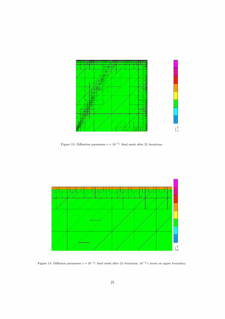
Figure 13: Diffustion parameter ε = 10−3: final mesh after 21 iterations.

Figure 14: Diffusion parameter ε = 10−3: final mesh after 21 iterations, 10−2× zoom on upper boundary.

21

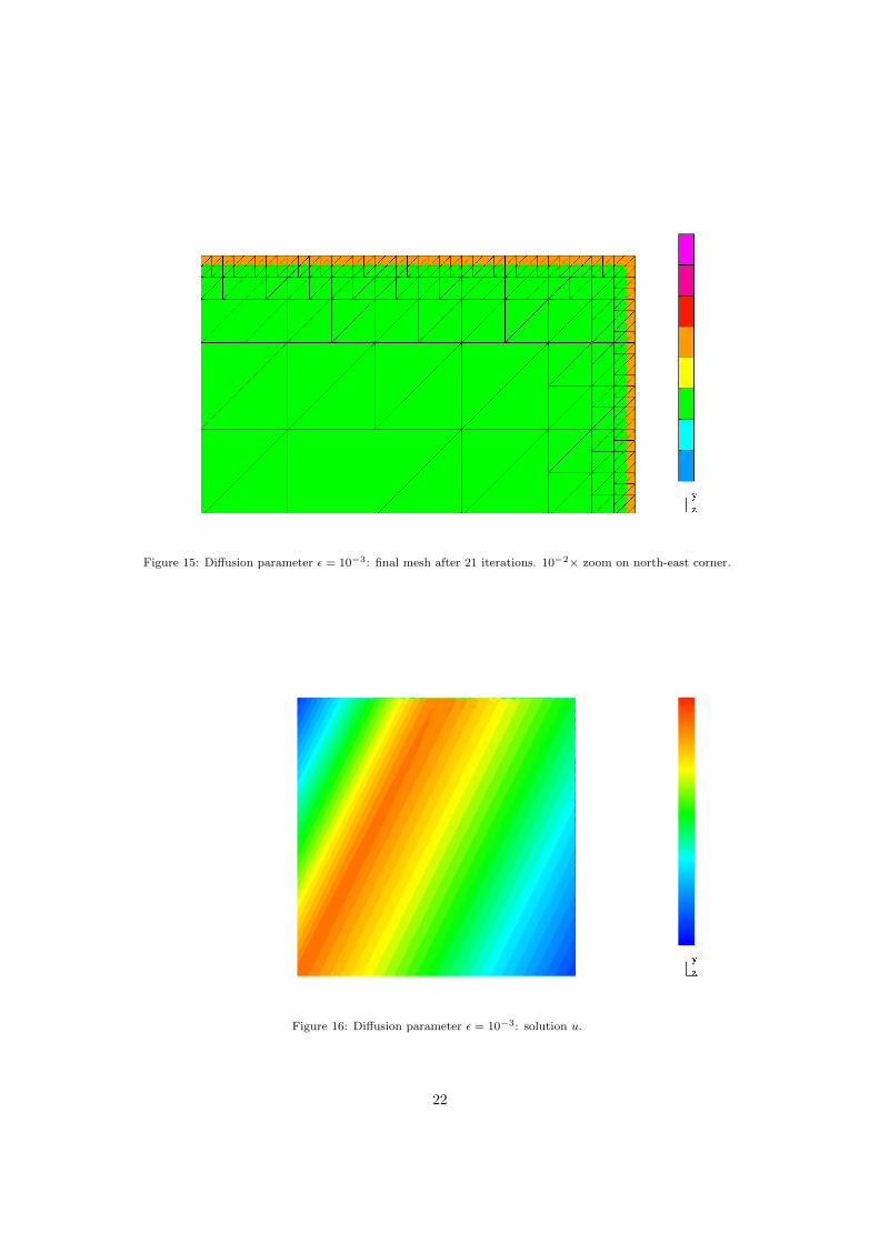
Figure 15: Diffusion parameter ε = 10−3: final mesh after 21 iterations. 10−2× zoom on north-east corner.

Figure 16: Diffusion parameter ε = 10−3: solution u.

22

Figure 17: Diffusion parameter ε = 10−3: solution u, 102× zoom on top boundary with the mesh.

Figure 18: Diffusion parameter ε = 10−3: solution u, 102× zoom on top boundary without the mesh.

23

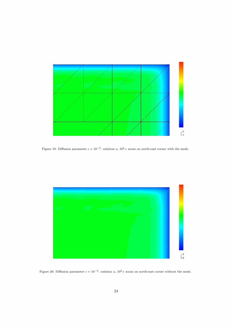
Figure 19: Diffusion parameter ε = 10−3: solution u, 102× zoom on north-east corner with the mesh.

Figure 20: Diffusion parameter ε = 10−3: solution u, 102× zoom on north-east corner without the mesh.

24

Here (σhp, uhp, σn, u) is the FE solution in the element, bK is the element bilinear form, (·, ·)K is the innerproduct for the test functions, and V (K), V (K) are the enriched spaces for determining the approximateoptimal test functions and the error representation functions. Once the functions (ψK , φK) are known, wedefine two directional contributions to the element error:

c1 :=

∫K

(|ψK,1|2 + |∂φK∂x1|2)w(x) dx c2 :=

∫K

(|ψK,2|2 + |∂φK∂x2|2)w(x) dx (4.69)

The anisotropy flag is defined now as follows:

Anisotropy flag =

10 if c1 ≥ 10c201 if c2 ≥ 10c111 otherwise

(4.70)

with the choice of factor 10 being arbitrary. The elements are refined according to their isotropy flags.If the flag points in one direction only, the element is h- or p-refined only in this direction. The for-mal algorithm is a slight modification of the algorithm for the triangular meshes and looks as follows:

Set δ = 0.5do while δ > 0.1solve the problem on the current mesh

for each element K in the mesh

compute element error contribution eK and isotropy flag

end of loop through elements

for each element K in the mesh

if eK > δ2 maxK eK then

if new h1, h2 ≥ ε then

h-refine the element

elseif new p, q ≤ pmax then

p-refine the element

endif

endif

end of loop through elements

if (new Ndof = old Ndof) reset δ = δ/2end of loop through mesh refinements

The ratio of maximum to minimum element size was limited to 10, 000. This number was determinedexperimentally in the process of determining the minimum diffusion parameter ε for which we can solve theproblem inspite of the conditioning problems. In the experiments with rectangular meshes, the advectionvector was changed to β = (1, 1). The corresponding solution is then symmetric along the diagonal so thatany loss of symmetry in the approximation points to either round off or programming errors.

Use of anisotropic refinements results in dramatic savings in terms of number of d.o.f. Fig. 21 presents theconvergence history for ε = 10−4. In place of the nearly 1M d.o.f. required for the triangles, the maximumnumber of d.o.f. reached only 134k. After 27 refinements, the energy error is reduced by four orders ofmagnitude (displayed is the error squared). As in the 1D examples, the error decreases monotonically.Slightly non-monotone behavior of the error in the last three iterations indicates that we are at the limitof machine precision. Quality of the solution obtained with the hp-refinements is illustrated in Fig. 22displaying the solution in the north-east corner of the square domain. The range for the computed solutionu is (−0.19044E − 04, 0.99980E + 00).

We have managed to solve the problem with ε = 10−5 by using additional restrictions on the elementaspect ratio (to 100) and rescaling the mass terms in the norm for the test functions by a factor of 10.However, limitation of the aspect ratio to 100 blowed up the number of d.o.f. to over 700k.

25

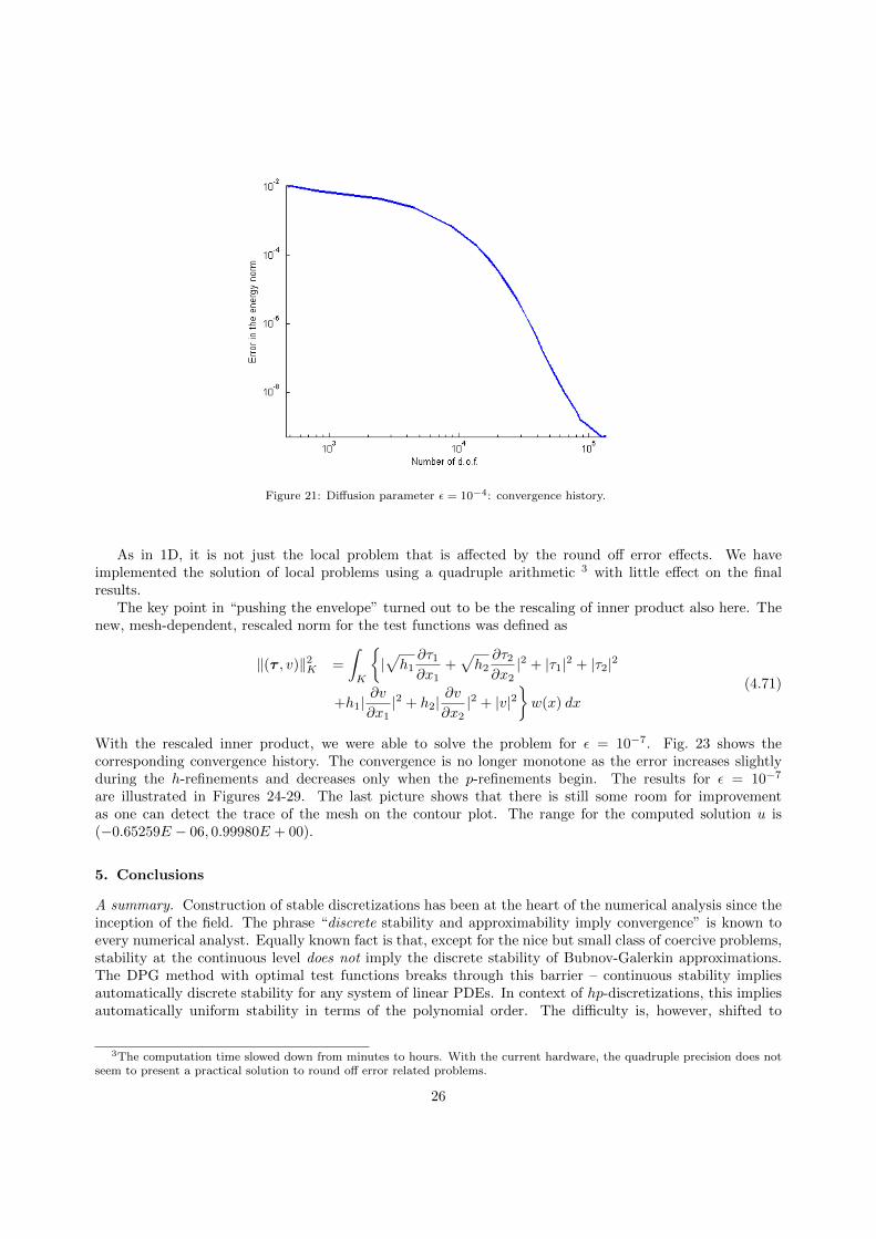
Figure 21: Diffusion parameter ε = 10−4: convergence history.

As in 1D, it is not just the local problem that is affected by the round off error effects. We haveimplemented the solution of local problems using a quadruple arithmetic 3 with little effect on the finalresults.

The key point in “pushing the envelope” turned out to be the rescaling of inner product also here. Thenew, mesh-dependent, rescaled norm for the test functions was defined as

‖(τ , v)‖2K =

∫K

|√h1∂τ1∂x1

+√h2∂τ2∂x2|2 + |τ1|2 + |τ2|2

+h1|∂v

∂x1|2 + h2|

∂v

∂x2|2 + |v|2

w(x) dx

(4.71)

With the rescaled inner product, we were able to solve the problem for ε = 10−7. Fig. 23 shows thecorresponding convergence history. The convergence is no longer monotone as the error increases slightlyduring the h-refinements and decreases only when the p-refinements begin. The results for ε = 10−7

are illustrated in Figures 24-29. The last picture shows that there is still some room for improvementas one can detect the trace of the mesh on the contour plot. The range for the computed solution u is(−0.65259E − 06, 0.99980E + 00).

5. Conclusions

A summary. Construction of stable discretizations has been at the heart of the numerical analysis since theinception of the field. The phrase “discrete stability and approximability imply convergence” is known toevery numerical analyst. Equally known fact is that, except for the nice but small class of coercive problems,stability at the continuous level does not imply the discrete stability of Bubnov-Galerkin approximations.The DPG method with optimal test functions breaks through this barrier – continuous stability impliesautomatically discrete stability for any system of linear PDEs. In context of hp-discretizations, this impliesautomatically uniform stability in terms of the polynomial order. The difficulty is, however, shifted to

3The computation time slowed down from minutes to hours. With the current hardware, the quadruple precision does notseem to present a practical solution to round off error related problems.

26

Figure 22: Diffusion parameter ε = 10−4: solution u, 103× zoom on the north-east corner.

Figure 23: Diffusion parameter ε = 10−7: convergence history.

27

Figure 24: Diffusion parameter ε = 10−7: hp mesh after 45 mesh refinements.

Figure 25: Diffusion parameter ε = 10−7: hp mesh after 45 mesh refinements, 102 − 105× zooms on the north-east corner.

28

Figure 26: Diffusion parameter ε = 10−7: velocity u.

Figure 27: Diffusion parameter ε = 10−7: velocity u, 105 zoom on the north-east corner.

29

Figure 28: Diffusion paramter ε = 10−7: velocity u, 106 zoom on the north-east corner with the mesh.

Figure 29: Diffusion parameter ε = 10−7: velocity u, 106 zoom on the north-east corner without the mesh.

30

proving uniform stability with respect to the mesh. The “natural” DPG energy norm is mesh-dependent, asit is for all DG methods and one of the first tasks in analyzing those methods is to establish a lower boundfor the mesh-dependent norm in terms of a global, mesh-independent norm.

We have established such a result for the 1D convection-dominated diffusion problem using the continuityof the error representation function. An alternative argument based on a concept of globally optimal testfunctions is presented in Appendix C.

With a proper choice of a weight for the norm in the test space, we have also managed to construct a “ro-bust” version of the method with stability properties uniform in the diffusion parameter ε. Construction of“robust” discretization schemes for singularly perturbed problems in general, and for convection-dominatedproblems in particular, has been a subject of an intensive research for decades, see [25] for a recent extensivereview of related work. Even the definition of what we mean by the ”robustness” is not easy. Intuitively,given a mesh, we expect the numerical solution to behave uniformly in terms of ε in an “eye-ball” normif the exact solution behaves so. For the 1D example studied in this paper, the L2-norm of both u andσ = εu′ can be bounded uniformly in ε, and we expect the same for the L2-norm of the corresponding FEerrors. As the first step towards a mathematically rigorous proof of robustness, we have proved that, with aproper choice of weight α, the L2 error of u, σ is bounded by the energy error of the group variable includingu, σ and the DPG fluxes u, σ. The method delivers the best approximation in the energy norm. In 1D,fluxes are just numbers and the best approximation of fluxes is thus always equal zero. Consequently, theL2 error of u, σ is bounded uniformly by the best approximation error of the same u, σ but in a different(the energy) norm. This does not automatically imply the robustness. The L2-error in u for the classicalBubnov-Galerkin method is bounded uniformly by the best approximation error of u measured in the H1

norm, but the method is not robust as the best approximation error measured in H1 norm blows up with ε(see [25] for a detailed discussion). In order to claim the robustness for the DPG method, we will need toestablish such a uniform bound for the best approximation error measured in the energy norm.

The choice of the test space norm also turned out to be a crucial tool in the fight against round offerror effects. With the rescaled norms, we have been able to extend the current limit of the diffusionparameter ε for which 2D problems can be solved with high-order elements on a double precision platformfrom to ε = 10−7. This “pushes the envelope” from DG results obtained by Houston et al. with predefinedgeometrically graded meshes [17] (Example 3 on page 2159, ε = 10−5) and more recent results of Zhu andSchotzau obtained in a fully adaptive mode [18] (Example 2 on page 28, ε = 0.510−5).

Most importantly, our adaptive process is fully automatic and it starts with few elements only. Themethod does not exhibit any preasymptotic range behavior where stability properties do not hold. In otherwords, one does not need to start with a mesh that reflects an expertise on the problem.

Convergence analysis in multi-dimensions. A careful examination of the arguments used in 1D to prove theglobal continuity of the error representation function reveals that we cannot count on the same result in2D or 3D. However, repeating the arguments, we learn that in place of continuity we have an orthogonalityresult: jump in error representation functions must be orthogonal to the trial space for fluxes. We have forinstance, ∫

e

[φK ]δuhp ds = 0 (5.72)

for every function δuhp from the trial space for edge e. Here [φK ] denotes the jump of the element errorrepresentation functions φK across the edge. See also Appendix C for related discussion on the relationbetween globally and locally optimal test functions.

An explicit computation of the energy norm in multi-dimensions does not seem possible, and we willhave to resort to a qualitative analysis only.

Current and future work. Besides the theoretical work, our current effort focuses on applying the DPGmethod to nonlinear problems - Burgers’ and compressible Navier-Stokes equations. We hope to presentnew exciting results in a forthcoming paper.

31

Additional comments added during the review process. The presented paper represents the state of ourknowledge at the time of the WONAPDE meeting (January 2010) where this work was presented. Sincethen we have made a significant progress on both theoretical and numerical sides. Among other results,in [26] we came up with a fundamental concept of the optimal test norm. With the use of the optimaltest norm, the corresponding energy norm is close to the original norm in the trial space, i.e. the L2-normfor the ”field” variables σ, u. This implies automatically a uniform bound of the L2-error by the energyerror, similarly to the result established in this paper using the weighted norms. For convection-dominateddiffusion however, the optimal test norm involves diffusion coefficient ε. Consequently, for large elementsused away from the boundary layer, determining optimal test functions becomes as difficult as solving theoriginal problem. The idea is not directly applicable to the “confusion” problems and the weighted testnorm remains to be our best choice. In [9], we delivered the first multidimensional analysis, for both Poissonand convection-dominated diffusion problems. The analysis went along different lines than predicted. Wemanaged to prove the mesh independence result but we are still unable to prove the robustness. Finally, themethod has been successfully extended to 1D compressible Navier–Stokes equations [27] using the weightednorms discussed here.

Acknowledgements

Demkowicz was supported in part by the Department of Energy [National Nuclear Security Administra-tion] under Award Number [DE-FC52-08NA28615], and by a research contract with Boeing. Gopalakrishnanwas supported in part by the National Science Foundation under grant DMS-0713833. Niemi was supportedin part by KAUST. We thank Bob Moser and David Young for encouragement and stimulating discussionson the project.

References

[1] L. Demkowicz, J. Gopalakrishnan, A class of discontinuous Petrov-Galerkin methods. Part II: Optimal test functions,Numer. Meth. Part. D. E.In print.

[2] J. Oden, L. Demkowicz, Applied Functional Analysis for Science and Engineering, Chapman & Hall/CRC Press, BocaRaton, 2010, second edition.

[3] I. Babuska, Error-bounds for finite element method, Numer. Math 16.[4] C. Bottasso, S. Micheletti, R. Sacco, The discontinuous Petrov-Galerkin method for elliptic problems, Comput. Methods

Appl. Mech. Engrg. 191 (2002) 3391–3409.[5] C. Bottasso, S. Micheletti, R. Sacco, A multiscale formulation of the discontinuous Petrov-Galerkin method for advective-

diffusive problems, Comput. Methods Appl. Mech. Engrg. 194 (2005) 2819–2838.[6] P. Causin, R. Sacco, A discontinuous Petrov-Galerkin method with Lagrangian multipliers for second order elliptic prob-

lems, SIAM J. Numer. Anal. 43.[7] P. Causin, R. Sacco, C. Bottasso, Flux-upwind stabilization of the discontinuous Petrov-Galerkin formulation with La-

grange multipliers for advection-diffusion problems, M2AN Math. Model. Numer. Anal. 39 (2005) 1087–1114.[8] L. Demkowicz, J. Gopalakrishnan, A class of discontinuous Petrov-Galerkin methods. Part I: The transport equation,

Comput. Methods Appl. Mech. Engrg.Accepted, see also ICES Report 2009-12.[9] L. Demkowicz, J. Gopalakrishnan, Analysis of the DPG method for the Poisson problem, Tech. Rep. 37, ICES, submitteed

to SIAM J. Num. Anal. (2010).[10] B. Cockburn, C.-W. Shu, TVB Runge-Kutta local projection discontinuous Galerkin finite element method for conservation

laws II: General framework, Mathematics of Computation 52.[11] B. Cockburn, C.-W. Shu, The local discontinuous Galerkin method for time-dependent convection-diffusion systems, SIAM

J. Num. Anal. 35 (1998) 2440–2463.[12] T. Hughes, A. Brooks, A multidimensional upwind scheme with no crosswind diffusion, in: Finite Element Methods for

Convection Dominated Flows (Papers, Winter Ann. Meeting Amer. Soc. Mech. Engrs., New York, 1979), Vol. 34 of AMD,Amer. Soc. Mech. Engrs. (ASME), New York, 1979, pp. 19–35.

[13] D. Arnold, F. Brezzi, M. Fortin, A stable finite element for the stokes equations, Calcolo 21 (4).[14] F. Brezzi, A. Russo, Choosing bubbles for advection-diffusion problems, Math. Models Methods Appl. Sci. 4.[15] F. Brezzi, L. Franca, A. Russo, Further considerations on residual free bubbles for advective-diffusive equations, Comput.

Methods Appl. Mech. Engrg. 166 (1998) 25–33.[16] P. Houston, C. Schwab, , E. Suli, Stabilized hp-finite element methods for first-order hyperbolic problems, SIAM J. Numer.

Anal. 37 (2000) 1618–1643, (electronic).[17] P. Houston, C. Schwab, , E. Suli, Discontinuous hp-finite element methods for advection-diffusion-reaction problems, SIAM

J. Numer. Anal. 39 (2002) 2133–2163.

32

[18] I. Zhu, Schotzau, A robust a posteriori error estimate for hp-adaptive dg methods for convection–diffusion equations, IMAJournal of Numerical Analysis (2010) 1–35Advance Access published April 28, 2010.

[19] J. Bramble, R. Lazarov, J. Pasciak, A least-squares approach based on a discrete minus one inner product for first ordersystems, Math. Comp 66.

[20] M. Ainsworth, J. Oden, A Posteriori Error Estimation in Finite Element Analysis, Wiley and Sons, Inc., New York, 2000.[21] L. Demkowicz, J. Oden, R. Rachowicz, A new finite element method for solving compressible Navier-Stokes equations

based on an operator splitting method and hp adaptivity, Comput. Methods Appl. Mech. Engrg. 84 (1990) 275–326.[22] C. Schwab, M. Suri, The p and hp versions of the finite element method for problems with boundary layers, Math. Comput.

65 (216) (1996) 1403–1429.[23] J. Melenk, hp-Finite Element Methods for Singular Perturbations, Springer, Berlin, 2002.[24] L. Demkowicz, Computing with hp Finite Elements. I.One- and Two-Dimensional Elliptic and Maxwell Problems, Chap-

man & Hall/CRC Press, Taylor and Francis, 2006.[25] H.-G. Roos, M. Stynes, L. Tobiska, Robust Numerical Methods for Singularly Perturbed Differential Equations, 2nd

Edition, Vol. 24 of Springer Series in Computational Mathematics, Springer-Verlag, Berlin, 2008.[26] J. Zitelli, I. Muga, L. Demkowicz, J. Gopalakrishnan, D. Pardo, V. Calo, A class of discontinuous Petrov-Galerkin methods.

Part IV: Wave propagation problems, Tech. Rep. 17, ICES, J. Comp. Phys., in review (2010).[27] J. Chan, L. Demkowicz, R. Moser, N. Roberts, A class of Discontinuous Petrov–Galerkin methods. Part V: Solution of 1d

Burgers and Navier–Stokes equations, Tech. Rep. 25, ICES, submitted to J. Comp. Phys. (2010).

Appendix A. Relation Between 1D Spectral and FE Energy Norms

In this section, we show that the global energy norm corresponding to norm (2.30), with a proper choiceof constants βk, is bounded below with the corresponding spectral norm of the solution premultiplied withorder 1 constant.

The local variational problems for determining optimal test functions look as follows.

∫ xk

xk−1

ατ ′δτ ′ + τ(xk)δτ(xk)

=1

ε

∫ xk

xk−1

σkδτ +

∫ xk

xk−1

ukδτ′ − (uδτ)|xkxk−1

∀δτ∫ xk

xk−1

αv′δv′ + βkv(xk)δv(xk)

=

∫ xk

xk−1

σkv′ − (σδv)|xkxk−1

−∫ xk

xk−1

ukv′ + (uδv)|xkxk−1

∀δv

(A.1)

For each flux unknown σ(xk), we have an optimal test function which spans across neighboring elements(xk−1, xk) and (xk, xk+1). For the first flux σ(0), the corresponding test function spans over the firstelement and, similarly, for the last flux σ(1), the corresponding test function spans over the last elementonly. Variational problem (A.1) leads to the following differential equations and boundary conditions forthe optimal test functions.

−(ατ ′)′ =1

εσk − u′k

α(xk)τ ′(xk) + βkτ(xk) = uk(xk)− u(xk)

−α(xk−1)τ ′(xk−1) = −uk(xk−1) + u(xk−1)

(A.2)

and −(αv′)′ = −σ′k + u′k

v′(xk) + βkv(xk) = σk(xk)− σ(xk)− uk(xk) + u(xk)

−v′(xk−1) = −σk(xk−1) + σ(xk−1) + uk(xk−1)− u(xk−1)

(A.3)

33

Solving for the optimal test functions, we obtain the following formula for the energy norm

‖(σ,u, σ, u)‖2E =

N∑k=1

[‖1

ε

∫ x

xk−1

σk(s) ds− uk(x) + u(xk−1)‖21/α + ‖ − σk(x) + uk(x) + σ(xk−1)− u(xk−1)‖21/α

]

+

N∑k=1

1

βk

[|1ε

∫ xk

xk−1

σk(s) ds− u|xkxk−1|2 + | − σ|xkxk−1

+ u|xkxk−1|2] (A.4)

with u(0) = u(1) = 0. More precisely,

σ = (σ1, . . . , σN )

u = (u1, . . . , uN )

σ = (σ(0), σ(x1), . . . , σ(1))

u = (u(x1), . . . , u(xN−1))

(A.5)

In order to simplify the notation, we will drop indices in field unknowns σk(x) = σ and uk(x) = u and someof the independent and integration variables,

‖(σ,u, σ, u)‖2E =

N∑k=1

[‖1

ε

∫ x

xk−1

σ − u+ u(xk−1)‖21/α + ‖ − σ + u+ σ(xk−1)− u(xk−1)‖21/α

]

+

N∑k=1

1

βk

[|1ε

∫ xk

xk−1

σ − u|xkxk−1|2 + | − σ|xkxk−1

+ u|xkxk−1|2] (A.6)

The element norms are weighted L2-norms with weight 1/α (inverse of the weight used for the norm of thetest functions).

We start with a simple estimate,

|1ε

∫ 1

0

σ| = |N∑k=1

(1

ε

∫ xk

xk−1

σ − u|xkxk−1

)|

≤N∑k=1

√βk

1√βk

∣∣∣∣∣1ε∫ xk

xk−1

σ − u|xkxk−1

∣∣∣∣∣≤ (

N∑k=1

βk)12

(N∑k=1

1

βk

∣∣∣∣∣1ε∫ xk

xk−1

σ − u|xkxk−1

∣∣∣∣∣) 1

2

(A.7)

The estimate suggests choosing βk = hk. In the same way,

|σ(1)− σ(0)| = |N∑k=1

(σ|xkxk−1− u|xkxk−1

)|

≤N∑k=1

√βk

1√βk|σ|xkxk−1

− u|xkxk−1|

≤ (

N∑k=1

βk)12

(N∑k=1

1

βk|σ|xkxk−1

− u|xkxk−1|2) 1

2

(A.8)

34

implies a similar estimate for |σ(1)− σ(0)|.Assume now that x ∈ (xk−1, xk), k > 1. We have,

−σ(x) + u(x) + σ(0) = −σ(x) + u(x) + σ(xk−1)− u(xk−1) +

k−1∑l−1

[−σ|xlxl−1

+ u|xlxl−1

](A.9)

which implies

∫ xk

xk−1

1

α|−σ+u+ σ(0)|2 ≤ 2

∫ xk

xk−1

1

α|−σ+u+ σ(xk−1)+ u(xk−1)|2 +2

hkαk

∣∣∣∣∣k−1∑l−1

[−σ|xlxl−1

+ u|xlxl−1

]∣∣∣∣∣2

(A.10)

where αk = minx∈(xk−1,xk) α(x), k > 1 is assumed to be finite.We use the discrete Cauchy-Schwarz inequality to estimate the second term on the right-hand side,

hkαk

∣∣∣∣∣k−1∑l−1

[−σ|xlxl−1

+ u|xlxl−1

]∣∣∣∣∣2

≤ hkαk

(k−1∑l=1

βl

) (k−1∑l−1

1

βl

∣∣∣−σ|xlxl−1+ u|xlxl−1

∣∣∣2) (A.11)

Taking into account that∑k−1l=1 βl = xk−1 and summing up the estimate in k, we get,∫ 1

0

1

α| − σ + u+ σ(0)|2 ≤ 2

N∑k=1

‖ − σ + u+ σ(xk−1) + u(xk−1)‖21/α

+2 maxk>1

∣∣∣∣xk−1

αk

∣∣∣∣(

N∑k=1

1

βk

[−σ|xkxk−1

+ u|xkxk−1

]) (A.12)

Notice that for α(x) = x, term xk−1

αk= 1.

We follow the same strategy to estimate the last term. Starting with identity for x ∈ (xk−1, xk), k > 1,

1

ε

∫ x

0

σ − u(x) =1

ε

∫ x

xk−1

σ − u(x) + u(xk−1) +

k−1∑l=1

[1

ε

∫ xl

xl−1

σ − u|xlxl−1

](A.13)

we obtain, ∫ 1

0

1

α|1ε

∫ x

0

σ − u(x)|2 ≤ 2

N∑k=1

‖∫ x

xk−1

σ − u+ u(xk−1)‖21/α

+2 maxk>1

∣∣∣∣xk−1

αk

∣∣∣∣ N∑k=1

1

βk

[1

ε

∫ xk

xk−1

σ − u|xkxk−1

]2 (A.14)

We can now formulate now our result.

THEOREM 1Consider an arbitrary (σ,u, σ, u) for which norm (A.4) is finite. Set constants βk = hk := xk − xk−1 andassume that the weight α(x) has been selected in such a way that minx∈(xk−1,xk) α(x) =: αk is finite, fork = 2, . . . , N . Let σ and u denote the unions of element functions σk, uk. Then the spectral energy normfor (σ, u, σ(0), σ(1)) is bounded by by the FE energy norm of (σ,u, σ, u),

‖1

ε

∫ x

0

σ − u‖21/α + ‖ − σ + u+ σ(0)‖21/α + |1ε

∫ 1

0

σ(s) ds|2 + | − σ(1) + σ(0)|2 ≤ C‖(σ,u, σ, u)‖2E (A.15)

where C = (1 + 2 max1,maxk>1xk−1

αk). For α(x) = x, C = 3.

35

Appendix B. Selection of Weight for 1D Convection-Dominated Problems

Assume a piecewise constant weight:

α(x) =

w 0 < x < y1 y < x < 1

We want to determine constant w and coordinate y in such a way that

|∫ 1

0

e−sε g(s) ds| ≤ Cε‖g‖1/α

with constant C independent of ε. Cauchy-Schwarz inequality implies that it is sufficient to select the weightin such a way that

‖e− sε ‖α ≤ Cε

Direct integration leads to the condition:

ε

2[1− e−

2yε ]w + [e−

2yε − e− 2

ε ] ≤ C2ε2

or, assuming C2 = 2,

[1− e−2yε ]w + [e−

2yε − e− 2

ε ] ≤ ε

We can request both terms in the sum above to be less than ε/2. In order to bound the second term, it issufficient to assume that

e−2yε ≤ ε

2

or, equivalently,

y ≥ − ε2

ln(ε

2)

Recall that the log function grows very slowly. For instance, for ε = 10−7, − ln(ε/2) ≈ 12. In order to boundthe first term by ε/2 it is sufficient to assume that w ≤ ε/2.

Appendix C. Globally and Locally Optimal Test Functions

Although the concept of optimal test functions is valid for any variational formulations, including thoseinvolving standard energy spaces, it is the DPG setting that makes the method practical. More precisely,critical is the use of discontinuous test functions (“broken” Sobolev spaces) which enables the local inversionof the Riesz operator. On the other side, the use of discontinuous test functions, and the resulting fluxes,makes the whole formulation mesh-dependent. The issue of mesh independence is, of course, fundamentalfor any h-convergence result.

In this appendix, we establish mesh independence of the energy norm for the 1D problem discussed inSection 2 using different means. Namely, we introduce the concept of globally optimal test functions anddiscuss their relation with optimal test functions for the DPG method which, for the sake of this discussion,we will identify now as locally optimal test functions. We shall use the 1D convection-dominated modelproblem for the discussion, but the conclusions made here apply to any 1D problem.

We begin with the variational formulation behind the one-element version of the DPG method.

σ, u ∈ L2(0, 1), σ(0), σ(1) ∈ IR

1

ε

∫ 1

0

στ +

∫ 1

0

uτ ′ = −u0τ(0) ∀τ ∈ H1(0, 1)

−∫ 1

0

σv′ − (σv)|10 −∫ 1

0

uv′ =

∫ 1

0

fv + u0v(0) ∀v ∈ H1(0, 1)

(C.1)

36

Notice that we do not use the term a spectral method which implies the use of polynomial trial functionsdefined on interval (0, 1). Instead, we assume that field unknowns σ, u will be approximated with hp trialbasis functions corresponding to a particular hp mesh. Contrary to polynomial bases, the hp trial functionsare discontinuous (still L2-conforming). We can use then the formulation, and the concept of optimal testfunctions, to introduce the corresponding globally optimal test functions. The optimal test functions aresolutions of the corresponding global variational problem,

τ, v ∈ H1(0, 1)∫ 1

0

τ ′δτ ′ + τδτ =1

ε

∫ 1

0

σδτ +

∫ 1

0

uδτ ′ ∀δτ ∈ H1(0, 1)∫ 1

0

vδv′ + vδv = −∫ 1

0

σδv′ − (σδv)|10 −∫ 1

0

uδv′ ∀δv ∈ H1(0, 1)

(C.2)

Above, σ, u and σ(0), σ(1) denote a particular trial function. In practice, the trial functions are scalar-valued, i.e. only one of the terms σ, u and σ(0), σ(1) is present. Notice that the optimal test function is,in general, vector-valued. The globally optimal test functions are H1(0, 1)-conforming which makes themglobally continuous. As a result of the global continuity of test functions, no interelement fluxes enter theformulation. The corresponding energy norm is mesh-independent. This the good news. The bad news isthat the optimal test functions are now global, spanning over the whole mesh. Their determination requiressolution of the global problem, and it is as expensive as the solution of the original problem. The resultingstiffness matrix is full and the method is no longer practical.

However, we can ask about the relation between the solutions obtained using the same set of trialfunctions, and the two sets of globally and locally optimal test functions. The global formulation deliversmesh-independence, the DPG version is practical. What is the relation between the two FE solutionscorresponding to the same set of trial functions? Let

0 = x0 < x1 < . . . xk < xk+1 < . . . xN = 1

be a FE mesh covering the domain (0, 1). Let σ, u and σ(0), σ(1) denote a particular trial basis functionscorresponding to the mesh, and let (τ, v) denote the corresponding globally optimal test function. As σ, uare smooth within each element (polynomials), variational boundary-value problem (C.2) translates into thefollowing differential equations, boundary and interface conditions for function τ ,

−τ ′′ + τ =1

εσ − u′ in (xk−1, xk), k = 1, . . . , N

[(τ ′ − u)(xk)] = 0 k = 1, . . . , N − 1

τ ′(1) = u(1)

−τ ′(0) = −u(0)

(C.3)

where [f(xk)] denotes the jump of f at xk. A similar set of conditions is satisfied by function v,

−v′′ + v = σ′ + u′ in (xk−1, xk), k = 1, . . . , N

[(v′ − σ + u)(xk)] = 0 k = 1, . . . , N − 1

v′(1) = σ(1)− σ(1)− u(1)

−v′(0) = −σ(0) = σ(0) + u(0)

(C.4)

Let δτ, δv ∈ ΠNk=1H

1(xk−1, xk), k = 1, . . . , N , be now a discontinuous test function. Multiplying (C.3)1 byδτ , integrating over each element, and summing up over all elements, we get,

N∑k=1

−∫ xk

xk−1

(τ ′ − u)′δτ +

∫ xk

xk−1

(τ − 1

εσ)δτ

= 0

37

Integrating the first term by parts, using the continuity of v′ + u at element interfaces, and boundaryconditions (C.3)3,4, we obtain,

N∑k=1

∫ xk

xk−1

τ ′δτ ′ + τδτ

=

N∑k=1

−∫ xk

xk−1

1

εσδτ + uδτ ′

+

N−1∑k=1

(τ ′ − u)(xk)[δτ(xk)] (C.5)

A similar result is obtained for the v-component of the globally optimal test function,

N∑k=1

∫ xk

xk−1

v′δv′ + vδv

=

N∑k=1

−∫ xk

xk−1

σv′ − uv′− (σδv)|10 +

N−1∑k=1

(v′ − σ + u)(xk)[δv(xk)] (C.6)

As the “broken” test functions (δτ, δv) are arbitrary, this proves that the globally optimal test function (τ, v)is a linear combination of the corresponding locally optimal test function corresponding to the same trialfunction σ, u, σ(1), σ(0), and locally optimal test functions corresponding to fluxes (τ ′−u)(xk), (v′−σ+u)(xk)at the interelement boundaries. This leads to the following result.

THEOREM 2Each globally optimal test function can be represented as a linear combination of locally optimal test functions.The globally optimal test functions form a subspace of locally optimal test functions. Consequently, thecorresponding FE solutions obtained using either the one element or the DPG setting, are identical.

The result extends to all 1D problems, but the situation in multidimensions is a bit different. Repeatingthe same reasoning in the 2D setting, we obtain the variational identities∑

K

∫K

divτ divδτ + τδτ

=∑K

−∫K

1

εσδτ + u divδτ

+∑e

∫e

(divτ − u)[δτn]∑K

∫K

∇v∇δv + vδv

=∑K

−∫K

σ∇v − βu∇v−∫∂K∩Γ

σnδv +∑e

∫e

(∂v

∂n− σn + βnu)[δv]

(C.7)

Here K denote elements, e interelement edges, β is the advection vector, and each interelement edge ecomes with a predefined normal ne necessary to define fluxes and normal advection vector component βn.Contrary to 1D, the interelement terms (divτ − u) and ( ∂v∂n − σn + βnu) can only be now approximatedwith flux trial functions. Consequently, the globally optimal test functions can only be approximated withlocally optimal test functions. With too low order for the fluxes, the inf-sup constant for the DPG methodis expected to deviate from the inf-sup constant for the one-element formulation.

This intuitively explains the relation of discretization for fluxes with the discretization for the fieldvariables. Increasing order of approximation for fluxes should only improve the global stability. If the ap-proximation for fluxes is insufficient (relative to the approximation for the field variables), we may loose meshindependence. The observation is illustrated with a numerical experiment for a 2D convection–dominateddiffusion problem. We use the data from Section 4 but, for a change, we replace the constant advection withthe incompressible velocity field β corresponding to potential φ,

φ = −x2 + y2, βx =∂φ

∂y, βy = −∂φ

∂x

Fig. C.30 presents solutions to the problem after 10 adaptive refinements for different combinations ofelement and flux orders. If p is the order for the field variables (σ1, σ2, u), the order for fluxes is set to(accounting for directionality),

pf = p+ ∆pf

with ∆pf = −1, 0, 1, 2. Diffusion constant is set to a moderate value of ε = 10−2, and we always startwith a mesh of four quadratic elements. Recall that our adaptive strategy is based on h-refinements with

38

Figure C.30: Convection-dominated diffusion in 2D: solutions after 10 adaptive steps corresponding to ∆pf = −1, 0, 1, 2.

polynomial order being raised only after the element size h drops below ε. Increasing order for fluxes makesthe method more expensive but, apparently, does not affect the global performance of the method. However,a further decrease of the order for fluxes to ∆pf = −2 (with p = 2, this means that fluxes are piecewiseconstant) resulted in a loss of mesh independence. Fig.C.31(a) presents the solution after three adaptiveh-refinements. Mesh independence is clearly lost and the refinements occur in a wrong place. However, thisdoes not contradict the p-convergence of the method for the same mesh as illustrated in Fig.C.31(b) whichpresents the solution after additional three p-refinements. The solution is not converged yet but it is clearlygoing in the right direction 4.

4Further increase in p was limited by the maximum order in our code pmax = 9 and the use of polynomials of order p+ 4for the enriched spaces.

39

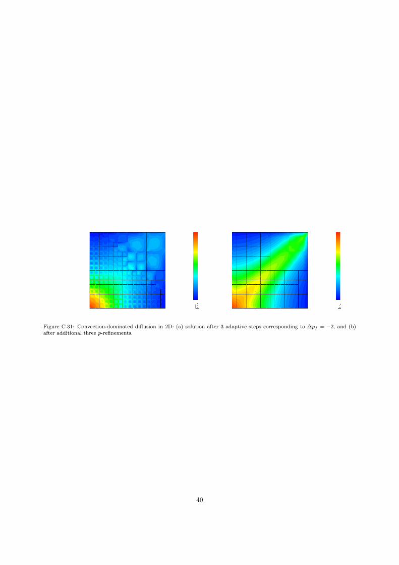
Figure C.31: Convection-dominated diffusion in 2D: (a) solution after 3 adaptive steps corresponding to ∆pf = −2, and (b)after additional three p-refinements.

40