High order direct discontinuous Galerkin method

Jue YanIowa State University

Lecture Series of High-Order Numerical MethodsJuly 27 – August 14, 2020

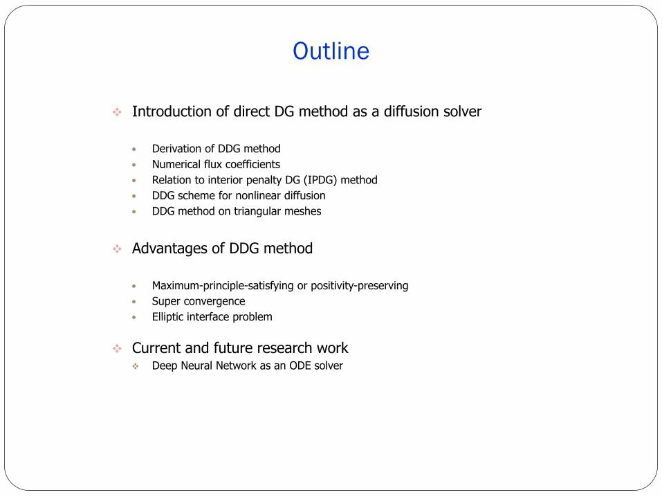
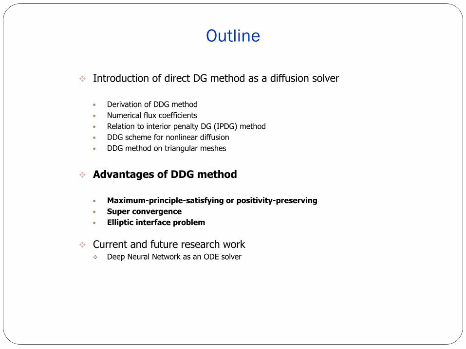
Outline

Introduction of direct DG method as a diffusion solver

Derivation of DDG method Numerical flux coefficients Relation to interior penalty DG (IPDG) method DDG scheme for nonlinear diffusion DDG method on triangular meshes

Advantages of DDG method

Maximum-principle-satisfying or positivity-preserving Super convergence Elliptic interface problem

Current and future research work Deep Neural Network as an ODE solver

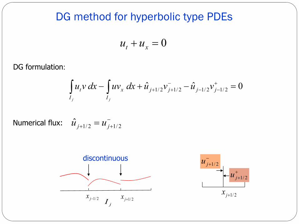
DG method for hyperbolic type PDEs

0=+ xt uu

0ˆˆ 2/12/12/12/1 =−+− +−−

−++∫∫ jjjj

Ix

It vuvudxuvdxvu

jj

−++ = 2/12/1ˆ jj uu

−+ 2/1ju

++ 2/1ju

2/1+jx

DG formulation:

Numerical flux:

jI

discontinuous

2/1+jx2/1−jx

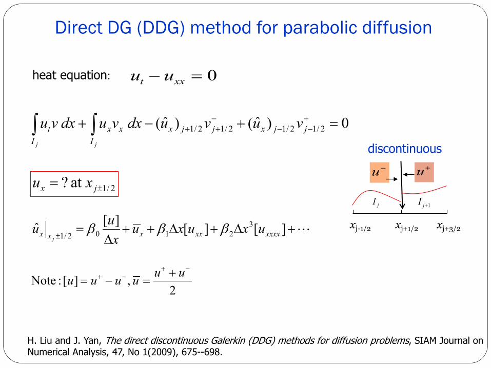
Direct DG (DDG) method for parabolic diffusion

+∆+∆++∆

=±

][][][ˆ 32102/1 xxxxxxxxx uxuxu

xuu

jβββ

2 ,][ :Note

−+−+ +

=−=uuuuuu

0=− xxt uuheat equation:

2/1at ? ±= jx xu−u +u

xj+3/2xj-1/2 xj+1/2

jI 1+jI

discontinuous

H. Liu and J. Yan, The direct discontinuous Galerkin (DDG) methods for diffusion problems, SIAM Journal on Numerical Analysis, 47, No 1(2009), 675--698.

0)ˆ()ˆ( 2/12/12/12/1 =+−+ +−−

−++∫∫ jjxjjx

Ixx

It vuvudxvudxvu

jj

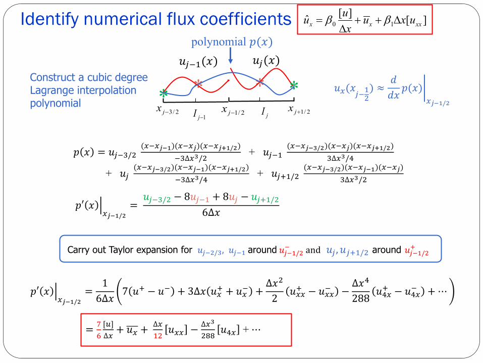
Identify numerical flux coefficients ][][ˆ 10 xxxx uxux

uu ∆++∆

= ββ

𝑢𝑢𝑥𝑥(𝑥𝑥𝑗𝑗−12

) ≈ 𝑑𝑑𝑑𝑑𝑥𝑥

𝑝𝑝(𝑥𝑥)𝑥𝑥𝑗𝑗−1/2

2/3−jx 2/1−jx**

2/1+jx

* *jI

1−jI

𝑢𝑢𝑗𝑗−1(𝑥𝑥) 𝑢𝑢𝑗𝑗(𝑥𝑥)polynomial 𝑝𝑝(𝑥𝑥)

Construct a cubic degree Lagrange interpolation polynomial

𝑝𝑝 𝑥𝑥 = 𝑢𝑢𝑗𝑗−3/2(𝑥𝑥−𝑥𝑥𝑗𝑗−1)(𝑥𝑥−𝑥𝑥𝑗𝑗)(𝑥𝑥−𝑥𝑥𝑗𝑗+1/2)

−3∆𝑥𝑥3/2+ 𝑢𝑢𝑗𝑗−1

(𝑥𝑥−𝑥𝑥𝑗𝑗−3/2)(𝑥𝑥−𝑥𝑥𝑗𝑗)(𝑥𝑥−𝑥𝑥𝑗𝑗+1/2)3∆𝑥𝑥3/4

+ 𝑢𝑢𝑗𝑗(𝑥𝑥−𝑥𝑥𝑗𝑗−3/2)(𝑥𝑥−𝑥𝑥𝑗𝑗−1)(𝑥𝑥−𝑥𝑥𝑗𝑗+1/2)

−3∆𝑥𝑥3/4+ 𝑢𝑢𝑗𝑗+1/2

(𝑥𝑥−𝑥𝑥𝑗𝑗−3/2)(𝑥𝑥−𝑥𝑥𝑗𝑗−1)(𝑥𝑥−𝑥𝑥𝑗𝑗)3∆𝑥𝑥3/2

𝑝𝑝′ 𝑥𝑥𝑥𝑥𝑗𝑗−1/2

=𝑢𝑢𝑗𝑗−3/2 − 8𝑢𝑢𝑗𝑗−1 + 8𝑢𝑢𝑗𝑗 − 𝑢𝑢𝑗𝑗+1/2

6∆𝑥𝑥

Carry out Taylor expansion for 𝑢𝑢𝑗𝑗−2/3, 𝑢𝑢𝑗𝑗−1 around 𝑢𝑢𝑗𝑗−1/2− and 𝑢𝑢𝑗𝑗 ,𝑢𝑢𝑗𝑗+1/2 around 𝑢𝑢𝑗𝑗−1/2

+

𝑝𝑝′ 𝑥𝑥𝑥𝑥𝑗𝑗−1/2

=1

6∆𝑥𝑥7 𝑢𝑢+ − 𝑢𝑢− + 3∆𝑥𝑥 𝑢𝑢𝑥𝑥+ + 𝑢𝑢𝑥𝑥− +

∆𝑥𝑥2

2𝑢𝑢𝑥𝑥𝑥𝑥+ − 𝑢𝑢𝑥𝑥𝑥𝑥− −

∆𝑥𝑥4

288𝑢𝑢4𝑥𝑥+ − 𝑢𝑢4𝑥𝑥− + ⋯

= 76

[𝑢𝑢]∆𝑥𝑥

+ 𝑢𝑢𝑥𝑥 + ∆𝑥𝑥12

𝑢𝑢𝑥𝑥𝑥𝑥 − ∆𝑥𝑥3

288𝑢𝑢4𝑥𝑥 + ⋯

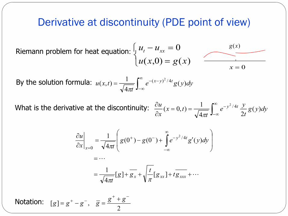
Derivative at discontinuity (PDE point of view)

Riemann problem for heat equation:

∫∞

∞−

−−= dyyget

txu tyx )(41),( 4/)( 2

π

==−

)()0,(0

xgxuuu xxt

0=x

)(xg

++++=

=

′+−=

∂∂

∫∞

∞−

−−+

=

xxxxxx

ty

x

gtgtggt

dyygeggtx

u

][][41

)()0()0(41 4/

0

2

ππ

π

By the solution formula:

What is the derivative at the discontinuity: ∫∞

∞−

−==∂∂ dyyg

tye

ttx

xu ty )(

241),0( 4/2

π

2 ,][

−+−+ +

=−=ggggggNotation:

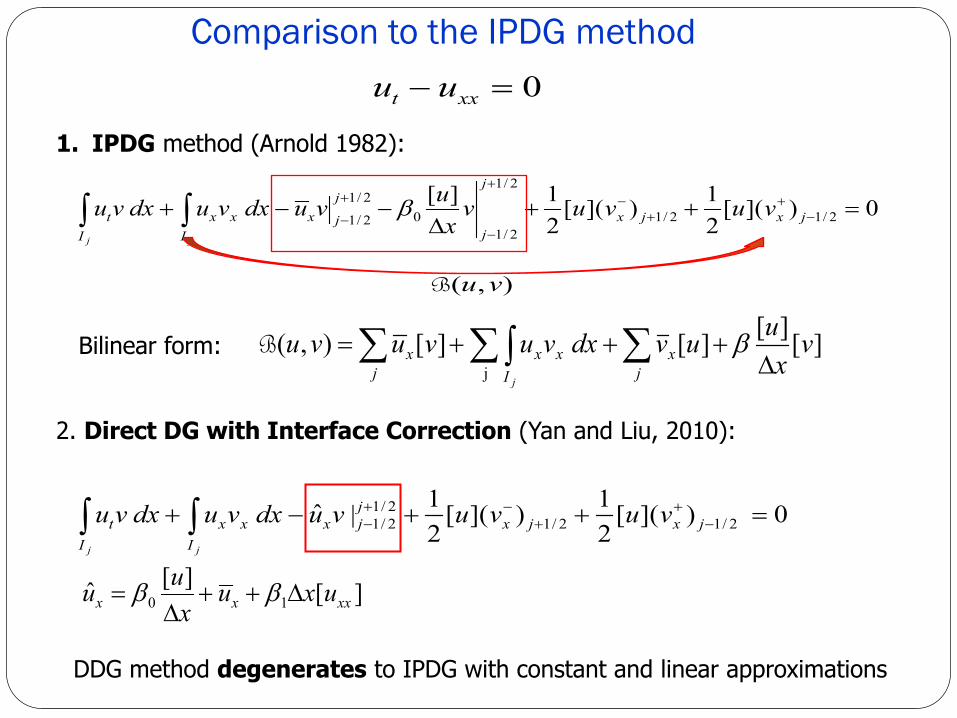
Comparison to the IPDG method

0 )]([21)]([

21 |ˆ 2/12/1

2/12/1 =++−+ −

++

−+−∫∫ jxjx

jjx

Ixx

It vuvuvudxvudxvu

jj

1. IPDG method (Arnold 1982):

2. Direct DG with Interface Correction (Yan and Liu, 2010):

0)]([21)]([

21][ 2/12/1

2/1

2/10

2/1

2/1=++

∆−−+ −

++

−+

−

+

−∫∫ jxjx

j

j

j

jxI

xxI

t vuvuvx

uvudxvudxvujj

β

][][ˆ 10 xxxx uxux

uu ∆++∆

= ββ

0=− xxt uu

DDG method degenerates to IPDG with constant and linear approximations

][][][ ][),(j

vx

uuvdxvuvuvuj

xI

xxj

x

j∆

+++= ∑∑ ∫∑ βBBilinear form:

),( vuB

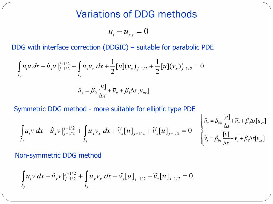
Variations of DDG methods 0=− xxt uu

0)]([21)]([

21 |ˆ 2/12/1

2/12/1 =+++− +

−−+

+− ∫∫ jxjx

Ixx

jjx

It vuvudxvuvudxvu

jj

][][ˆ 10 xxxx uxux

uu ∆++∆

= ββ

DDG with interface correction (DDGIC) – suitable for parabolic PDE

Symmetric DDG method - more suitable for elliptic type PDE

Non-symmetric DDG method

0][~][~ |ˆ 2/12/12/12/1 =+++− −+

+− ∫∫ jxjx

Ixx

jjx

It uvuvdxvuvudxvu

jj

∆++∆

=

∆++∆

=

][][~

][][ˆ

10

10

xxxvx

xxxux

vxvx

vv

uxux

uu

ββ

ββ

0][~][~ |ˆ 2/12/12/12/1 =−−+− −+

+− ∫∫ jxjx

Ixx

jjx

It uvuvdxvuvudxvu

jj

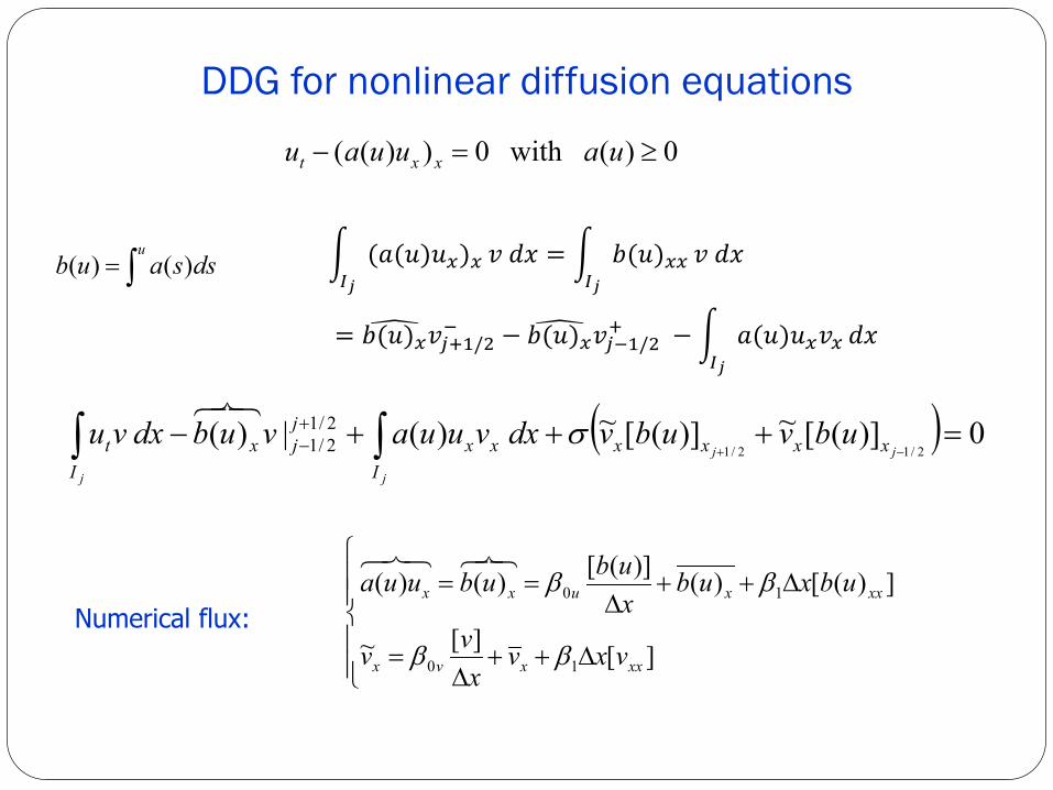
DDG for nonlinear diffusion equations

0)( with 0))(( ≥=− uauuau xxt

∫=u

dssaub )()(

∆++∆

=

∆++∆

==

][][~

])([)()]([)()(

10

10

xxxvx

xxxuxx

vxvx

vv

ubxubxububuua

ββ

ββ

( ) 0)]([~)]([~ )( |)( 2/12/1

2/12/1 =+++−

−+∫∫ +− jj

jj

xxxxI

xxjjx

It ubvubvdxvuuavubdxvu σ

𝐼𝐼𝑗𝑗

(𝑎𝑎(𝑢𝑢)𝑢𝑢𝑥𝑥)𝑥𝑥 𝑣𝑣 𝑑𝑑𝑥𝑥 = 𝐼𝐼𝑗𝑗𝑏𝑏(𝑢𝑢)𝑥𝑥𝑥𝑥 𝑣𝑣 𝑑𝑑𝑥𝑥

= 𝑏𝑏(𝑢𝑢)𝑥𝑥𝑣𝑣𝑗𝑗+1/2− − 𝑏𝑏(𝑢𝑢)𝑥𝑥𝑣𝑣𝑗𝑗−1/2

+ − 𝐼𝐼𝑗𝑗𝑎𝑎(𝑢𝑢)𝑢𝑢𝑥𝑥𝑣𝑣𝑥𝑥 𝑑𝑑𝑥𝑥

Numerical flux:

0=∆− uut

DDGIC scheme:

Numerical flux:

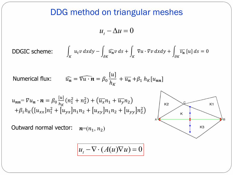
DDG method on triangular meshes

𝐾𝐾𝑢𝑢𝑡𝑡𝑣𝑣 𝑑𝑑𝑥𝑥𝑑𝑑𝑑𝑑 −

𝜕𝜕𝐾𝐾𝑢𝑢𝒏𝒏𝑣𝑣 𝑑𝑑𝑠𝑠 +

𝐾𝐾∇𝑢𝑢 𝛻𝛻𝑣𝑣 𝑑𝑑𝑥𝑥𝑑𝑑𝑑𝑑 +

𝜕𝜕𝐾𝐾𝑣𝑣𝐧𝐧 [𝑢𝑢]𝑑𝑑𝑠𝑠 = 0

𝑢𝑢𝒏𝒏 = ∇𝑢𝑢 𝒏𝒏 = 𝛽𝛽0[𝑢𝑢]ℎ𝐾𝐾

+ 𝑢𝑢𝒏𝒏 +𝛽𝛽1 ℎ𝐾𝐾[𝑢𝑢𝒏𝒏𝒏𝒏]

𝑢𝑢𝒏𝒏𝒏𝒏= 𝛻𝛻𝑢𝑢𝒏𝒏 𝒏𝒏 = 𝛽𝛽0𝑢𝑢ℎ𝐾𝐾

𝑛𝑛12 + 𝑛𝑛22 + 𝑢𝑢𝑥𝑥𝑛𝑛1 + 𝑢𝑢𝑦𝑦𝑛𝑛2+𝛽𝛽1ℎ𝐾𝐾 𝑢𝑢𝑥𝑥𝑥𝑥 𝑛𝑛12 + 𝑢𝑢𝑦𝑦𝑥𝑥 𝑛𝑛1𝑛𝑛2 + 𝑢𝑢𝑥𝑥𝑦𝑦 𝑛𝑛1𝑛𝑛2 + 𝑢𝑢𝑦𝑦𝑦𝑦 𝑛𝑛22

𝒏𝒏=(𝑛𝑛1, 𝑛𝑛2)Outward normal vector:

0))(( =∇⋅∇− uuAut

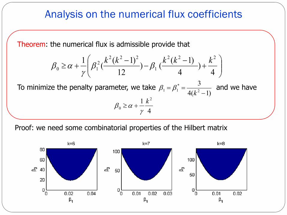
Analysis on the numerical flux coefficients

+

−−

−+≥

4)

4)1(()

12)1((1 222

1

2222

10kkkkk ββ

γαβ

Theorem: the numerical flux is admissible provide that

To minimize the penalty parameter, we take and we have)1(4

32

*11 −==

kββ

41 2

0k

γαβ +≥

Proof: we need some combinatorial properties of the Hilbert matrix

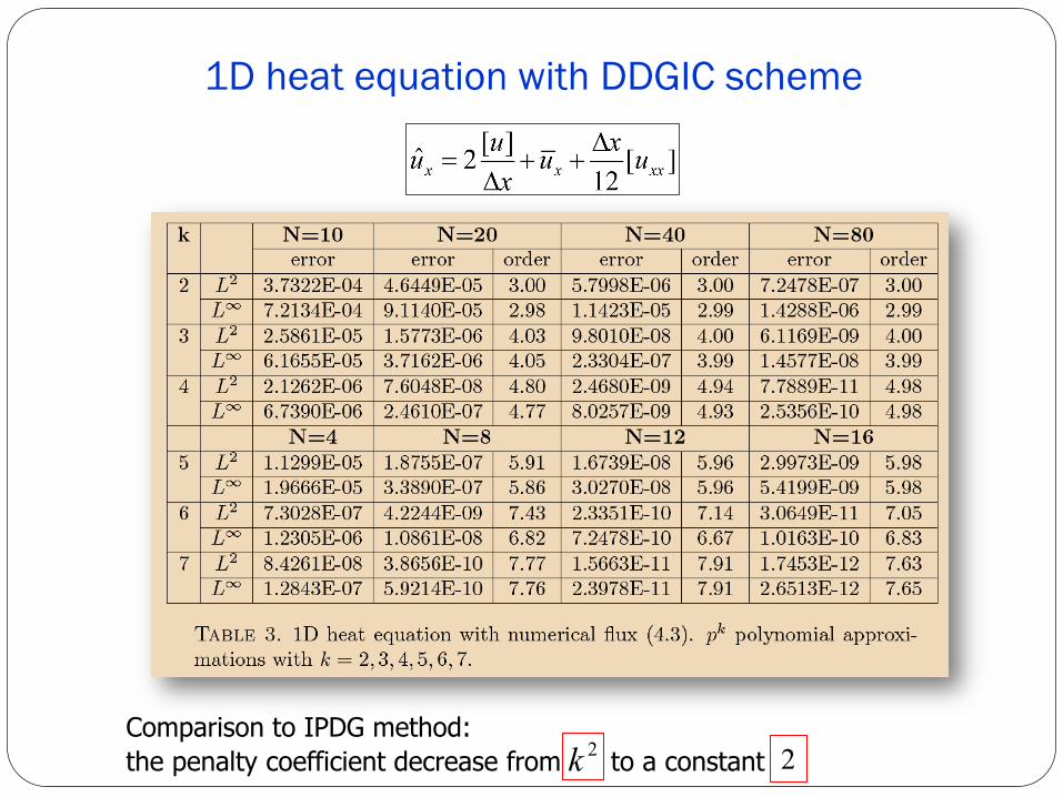
1D heat equation with DDGIC scheme

Comparison to IPDG method: the penalty coefficient decrease from to a constant 2k 2

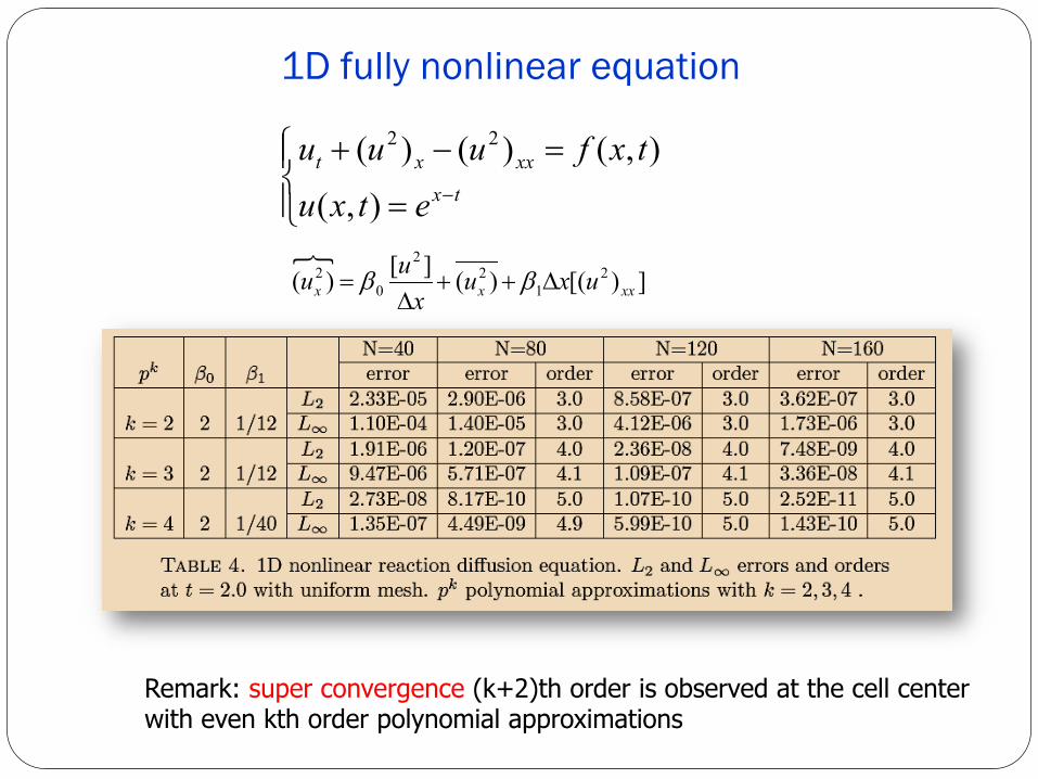
1D fully nonlinear equation

=

=−+−tx

xxxt

etxutxfuuu

),(),()()( 22

])[()(][)( 2

12

2

02

xxxx uxux

uu ∆++∆

= ββ

Remark: super convergence (k+2)th order is observed at the cell center with even kth order polynomial approximations

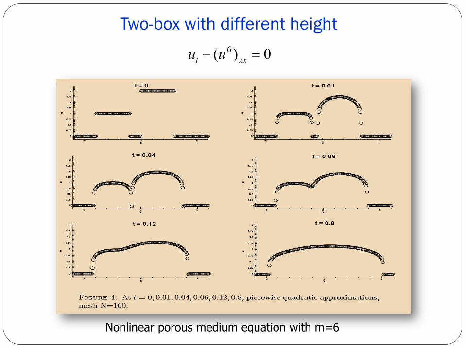
Two-box with different height

Nonlinear porous medium equation with m=6

0)( 6 =− xxt uu

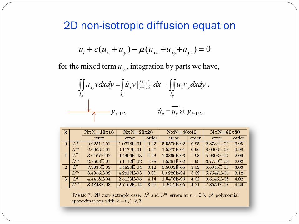
2D non-isotropic diffusion equation

0)()( =++−++ yyxyxxyxt uuuuucu µ

have, wepartsby nintegratio , termmixed for the xyu

. dxdyvudxvuvdxdyuijiij I

yxI

jjx

Ixy ∫∫∫∫∫ −= +

−2/12/1|ˆ

2/1+jy .at ˆ 2/1±= jxx yuu

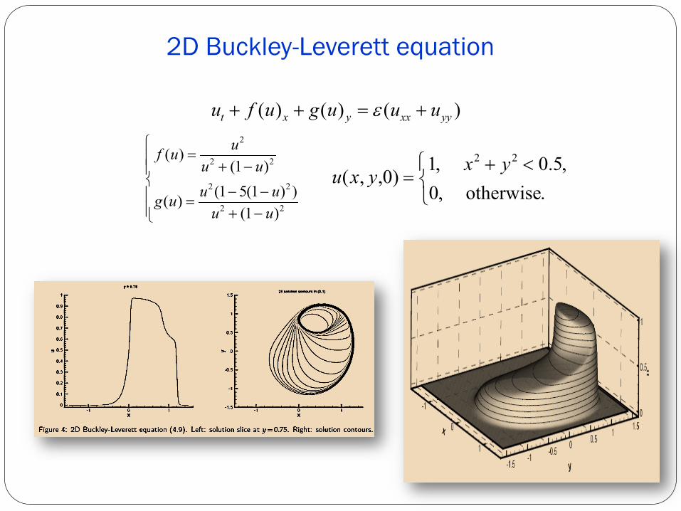
2D Buckley-Leverett equation

)()()( yyxxyxt uuugufu +=++ ε

−+−−

=

−+=

22

22

22

2

)1())1(51()(

)1()(

uuuuug

uuuuf

<+

=.otherwise ,0

,5.0 ,1)0,,(

22 yxyxu

Outline

Introduction of direct DG method as a diffusion solver

Derivation of DDG method Numerical flux coefficients Relation to interior penalty DG (IPDG) method DDG scheme for nonlinear diffusion DDG method on triangular meshes

Advantages of DDG method

Maximum-principle-satisfying or positivity-preserving Super convergence Elliptic interface problem

Current and future research work Deep Neural Network as an ODE solver

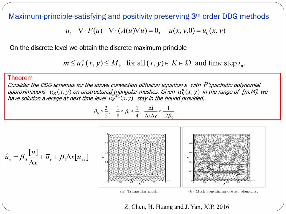
Maximum-principle-satisfying and positivity preserving 3rd order DDG methods

),()0,,( ,0))(()( 0 yxuyxuuuAuFut ==∇⋅∇−⋅∇+

On the discrete level we obtain the discrete maximum principle

. step timeand ),( allfor ,),( nnK tKyxMyxum Ω∈∈≤≤

2P

.12

1yx

t ,41

81 ,

23

010 βββ ≤

∆∆∆

≤≤≥

TheoremConsider the DDG schemes for the above convection diffusion equation s with quadratic polynomial approximations on unstructured triangular meshes. Given in the range of [m,M], we have solution average at next time level stay in the bound provided,

][][ˆ 10 xxxx uxux

uu ∆++∆

= ββ

𝑢𝑢𝐾𝐾(𝑥𝑥,𝑑𝑑) 𝑢𝑢𝐾𝐾𝑛𝑛(𝑥𝑥,𝑑𝑑)𝑢𝑢𝐾𝐾𝑛𝑛+1(𝑥𝑥,𝑑𝑑)

Z. Chen, H. Huang and J. Yan, JCP, 2016

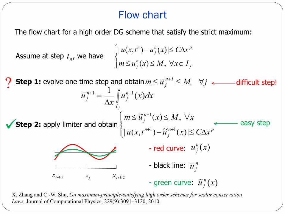
Flow chart The flow chart for a high order DG scheme that satisfy the strict maximum:

∈∀≤≤

∆≤−

jnj

pnj

n

IxMxum

xCxutxu

,)(

|)(),(| Assume at step , we have

Step 1: evolve one time step and obtain

Step 2: apply limiter and obtain

jM, um 1nj ∀≤≤ +

nt

∆≤−

∀≤≤++

+

pnj

n

nj

xCxutxu

xMxum

|)(~),(|

,)(~

11

1

∫ ++

∆=

jI

nj

nj dxxu

xu )(1 11

difficult step!

easy step

2/1−jx 2/1+jxjx

- red curve:

- black line:

- green curve:

)(xunj

)(~ xu nj

nju

X. Zhang and C.-W. Shu, On maximum-principle-satisfying high order schemes for scalar conservationLaws, Journal of Computational Physics, 229(9):3091–3120, 2010.

?

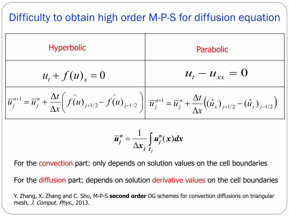
Difficulty to obtain high order M-P-S for diffusion equation

For the convection part: only depends on solution values on the cell boundaries

0)( =+ xt ufu

)()( 2/12/11

−

∆∆

+= −

∧

+

∧+

jjnj

nj ufuf

xtuu ( ) )ˆ()ˆ( 2/12/1

1−+

+ −∆∆

+= jxjxnj

nj uu

xtuu

Hyperbolic Parabolic

0=− xxt uu

For the diffusion part: depends on solution derivative values on the cell boundaries

Y. Zhang, X. Zhang and C. Shu, M-P-S second order DG schemes for convection diffusions on triangular mesh, J. Comput. Phys., 2013.

∫∆=

jI

nj

j

nj dxxu

xu )(1

( ) ))(),(),(( )ˆ()ˆ( 112/12/11 xuxuxuHuu

xtuu n

jnj

njjxjx

nj

nj +−−++ =−

∆∆

+=

2/1−jx 2/1+jx

***

)(xunj

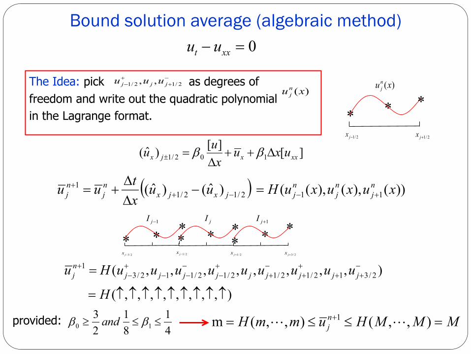
Bound solution average (algebraic method)

2/1+jx

***

2/3+jx

***

2/3−jx 2/1−jx

***

jI 1+jI1−jI

The Idea: pick as degrees of freedom and write out the quadratic polynomial in the Lagrange format.

)(xunj

−+

+− 2/12/1 ,, jjj uuu

),,,,,,,,(

),,,,,,,,( 2/312/12/12/12/112/31

↑↑↑↑↑↑↑↑↑=

= −++

++

−+

+−

−−−

+−

+

H

uuuuuuuuuHu jjjjjjjjjnj

MMMHummH nj =≤≤= + ),,( ),,(m 1

41

81

23

10 ≤≤≥ ββ and

][][)ˆ( 102/1 xxxjx uxux

uu ∆++∆

=± ββ

provided:

0=− xxt uu

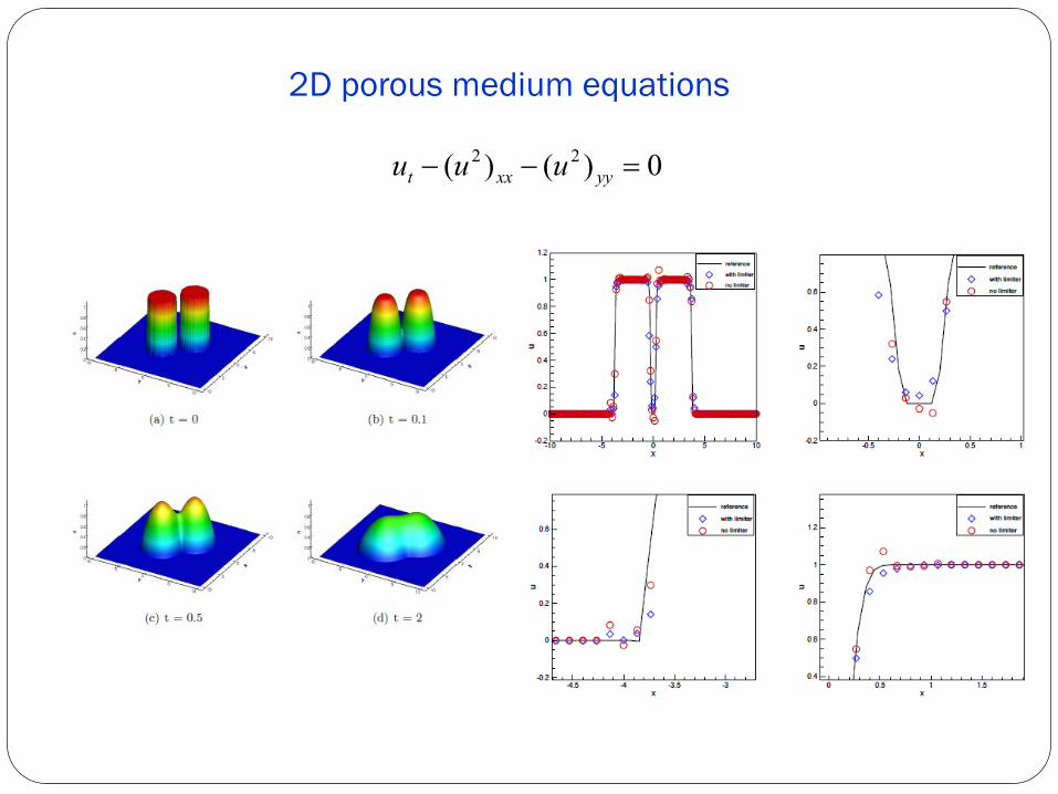
2D porous medium equations

0)()( 22 =−− yyxxt uuu

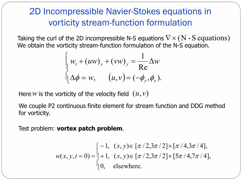
2D Incompressible Navier-Stokes equations in vorticity stream-function formulation

( )

−==∆

∆=++

).,(, ,Re1)()(

xy

yxt

vuw

wvwuww

φφφ

Test problem: vortex patch problem.

We couple P2 continuous finite element for stream function and DDG method for vorticity.

Here is the vorticity of the velocity field ),( vuw

Taking the curl of the 2D incompressible N-S equations We obtain the vorticity stream-function formulation of the N-S equation.

)equations S-N(×∇

×∈+×∈−

==.elsewhere ,0

],4/7,4/5[]2/3,2/[),( ,1],4/3,4/[]2/3,2/[),( ,1

)0,,( ππππππππ

yxyx

tyxw

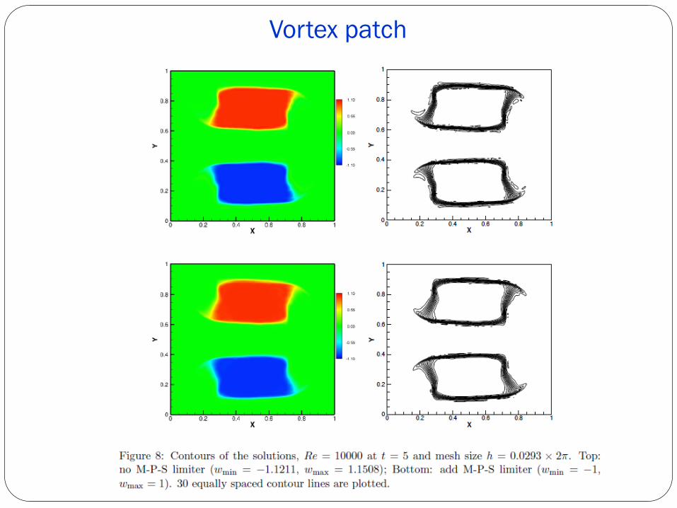
Vortex patch

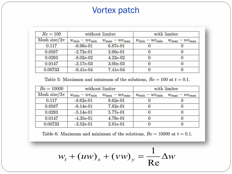
Vortex patch

wvwuww yxt ∆=++Re1)()(

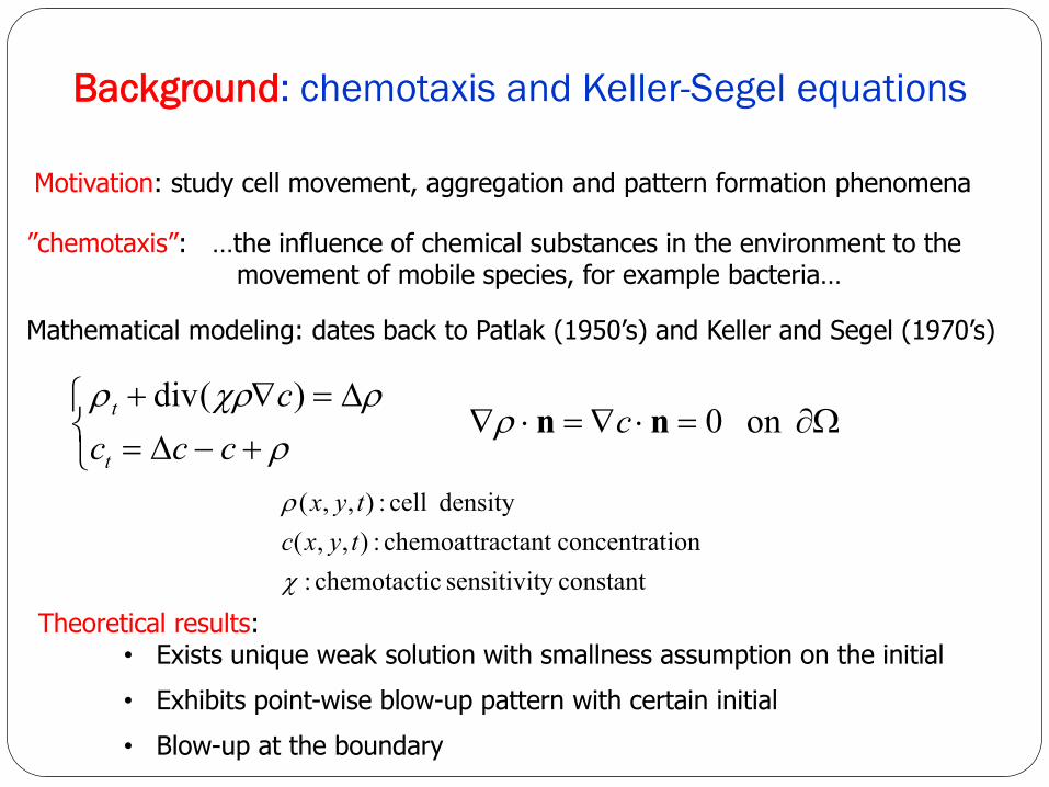
Background: chemotaxis and Keller-Segel equations

Motivation: study cell movement, aggregation and pattern formation phenomena

”chemotaxis”: …the influence of chemical substances in the environment to the movement of mobile species, for example bacteria…

Mathematical modeling: dates back to Patlak (1950’s) and Keller and Segel (1970’s)

Ω∂=⋅∇=⋅∇

+−∆=∆=∇+

on 0 )(div

nn cccc

c

t

t ρρ

ρχρρ

constanty sensitivit cchemotacti :ionconcentratctant chemoattra :),,(

density cell :),,(

χ

ρtyxctyx

Theoretical results: • Exists unique weak solution with smallness assumption on the initial• Exhibits point-wise blow-up pattern with certain initial• Blow-up at the boundary

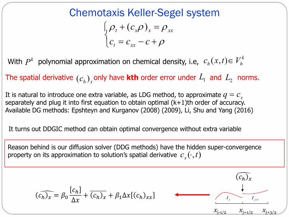
Chemotaxis Keller-Segel system

+−==+ρρρρ

cccc

xxt

xxxxt )(

With polynomial approximation on chemical density, i.e, kP khh Vtxc ∈),(

xhc )(The spatial derivative only have kth order error under and norms.1L 2L

It is natural to introduce one extra variable, as LDG method, to approximate separately and plug it into first equation to obtain optimal (k+1)th order of accuracy.Available DG methods: Epshteyn and Kurganov (2008) (2009), Li, Shu and Yang (2016)

xcq =

It turns out DDGIC method can obtain optimal convergence without extra variable

Reason behind is our diffusion solver (DDG methods) have the hidden super-convergence property on its approximation to solution’s spatial derivative ),( tcx ⋅

xj+3/2xj-1/2 xj+1/2

jI 1+jI𝑐𝑐ℎ 𝑥𝑥 = 𝛽𝛽0

𝑐𝑐ℎ∆𝑥𝑥

+ 𝑐𝑐ℎ 𝑥𝑥 + 𝛽𝛽1∆𝑥𝑥 𝑐𝑐ℎ 𝑥𝑥𝑥𝑥

𝑐𝑐ℎ 𝑥𝑥

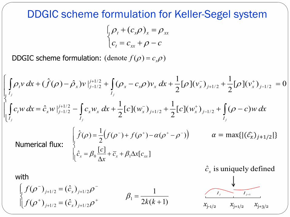
DDGIC scheme formulation for Keller-Segel system

−+==+

cccc

xxt

xxxxt

ρρρρ )(

−+++−=

=++−+−+

∫∫∫

∫∫

−+

+−+

−

−+

+−+

−

)()]([21)]([

21 |ˆ

0 )]([21)]([

21 )( |)ˆ)(ˆ(

2/12/12/12/1

2/12/12/12/1

dxwcwcwcdxwcwcdxwc

vvdxvcvfdxv

jjj

jj

Ijxjxx

Ix

jjx

It

jxjxxxI

xjjx

It

ρ

ρρρρρρρ

( )

∆++∆

=

−−+= −++−

][][ˆ

)()()(21)(ˆ

10 xxxx cxcx

cc

fff

ββ

ρραρρρ

DDGIC scheme formulation:

Numerical flux:

with

=

=+

+++

−++

−

ρρ

ρρ

2/12/1

2/12/1

)ˆ()(

)ˆ()(

jxj

jxj

cf

cf

xj+3/2xj-1/2 xj+1/2

jI 1+jI

defineduniquely is ˆxc

)1(21

1 +=

kkβ

))( denote( ρρ xcf =

𝛼𝛼 = max|( 𝑐𝑐𝑥𝑥)𝑗𝑗+1/2|

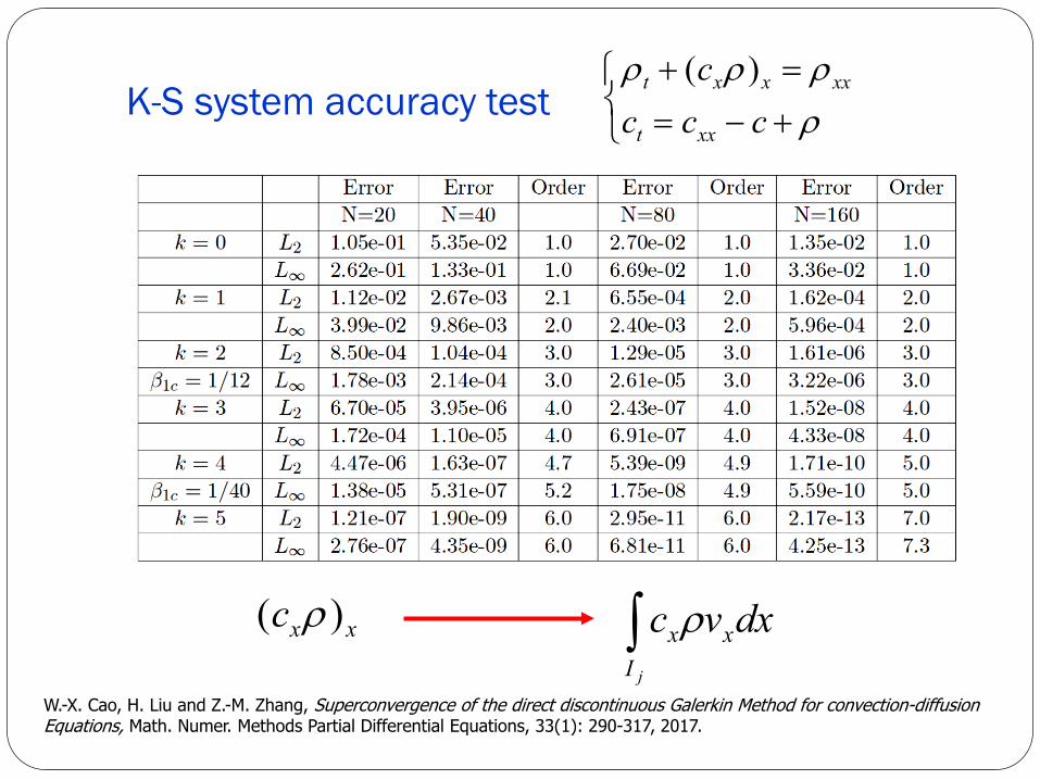
K-S system accuracy test

+−==+ρρρρ

cccc

xxt

xxxxt )(

xxc )( ρ ∫jI

xx dxvc ρ

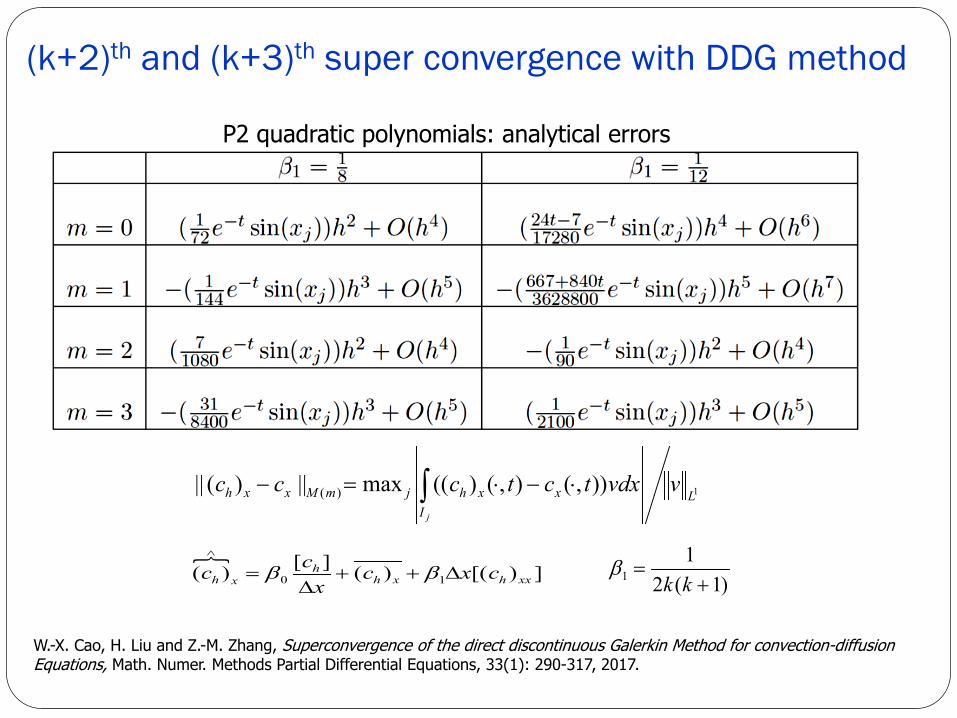
W.-X. Cao, H. Liu and Z.-M. Zhang, Superconvergence of the direct discontinuous Galerkin Method for convection-diffusion Equations, Math. Numer. Methods Partial Differential Equations, 33(1): 290-317, 2017.

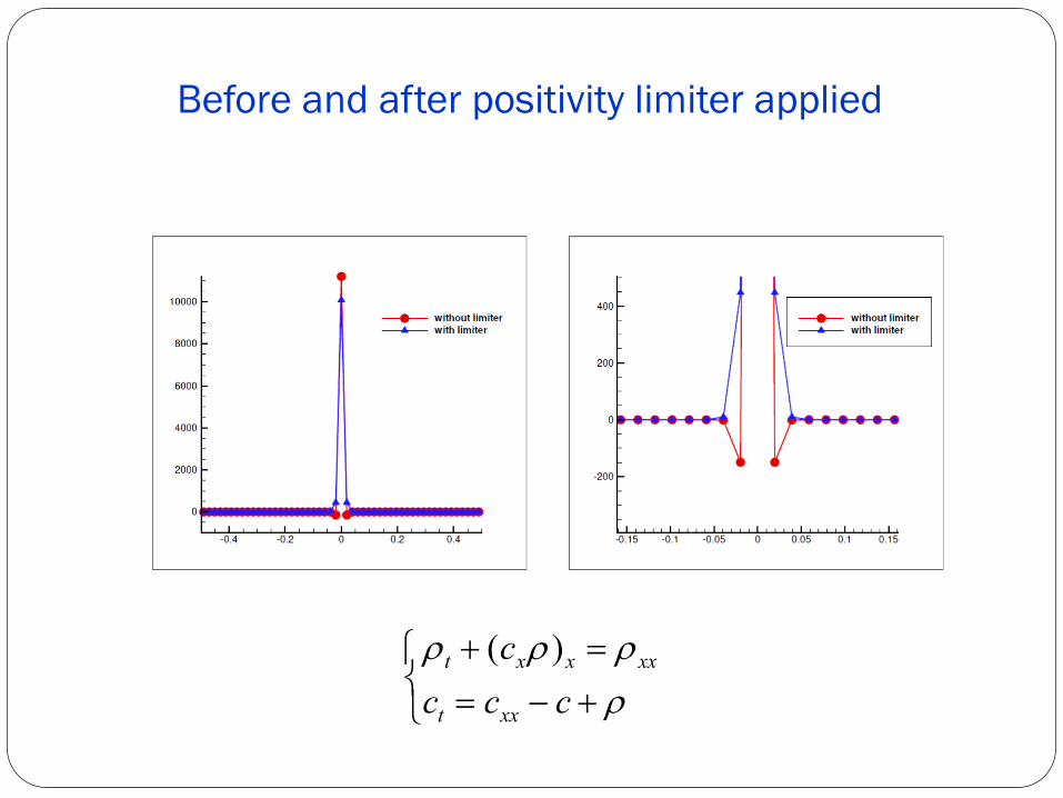
Before and after positivity limiter applied

+−==+ρρρρ

cccc

xxt

xxxxt )(

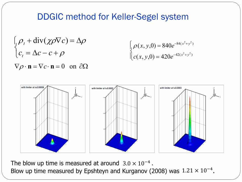
DDGIC method for Keller-Segel system

)(div

+−∆=∆=∇+

ρρχρρ

cccc

t

t

Ω∂=⋅∇=⋅∇ on 0nn cρ

420)0,,(

840)0,,()(42

)(84

22

22

=

=+−

+−

yx

yx

eyxc

eyxρ

The blow up time is measured at around . Blow up time measured by Epshteyn and Kurganov (2008) was .

3.0 × 10−41.21 × 10−4

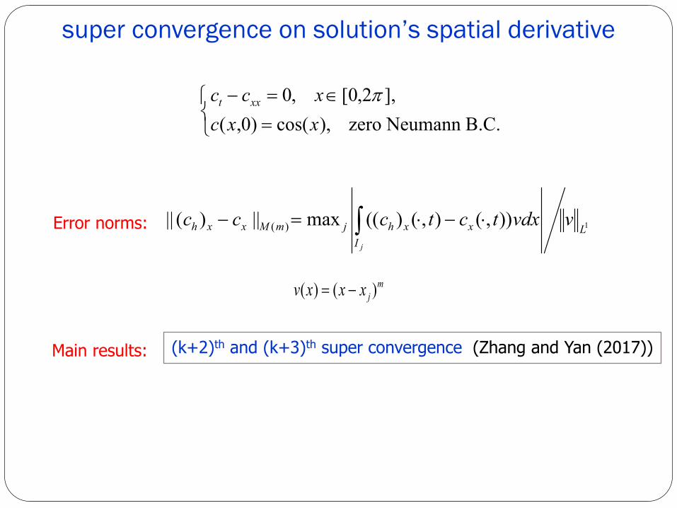
super convergence on solution’s spatial derivative

Error norms:

=∈=−

B.C.Neumann zero ),cos()0,(],2,0[ ,0

xxcxcc xxt π

1)),(),()((max||)(|| )( LI

xxhjmMxxh vvdxtctcccj

∫ ⋅−⋅=−

mjxxxv )()( −=

(k+2)th and (k+3)th super convergence (Zhang and Yan (2017)) Main results:

])[()(][)( 10 xxhxh

hxh cxc

xcc ∆++∆

=∧

ββ

(k+2)th and (k+3)th super convergence with DDG method

P2 quadratic polynomials: analytical errors

1)),(),()((max||)(|| )( LI

xxhjmMxxh vvdxtctcccj

∫ ⋅−⋅=−

)1(21

1 +=

kkβ

W.-X. Cao, H. Liu and Z.-M. Zhang, Superconvergence of the direct discontinuous Galerkin Method for convection-diffusion Equations, Math. Numer. Methods Partial Differential Equations, 33(1): 290-317, 2017.

])[()(][)( 10 xxhxh

hxh cxc

xcc ∆++∆

=∧

ββ

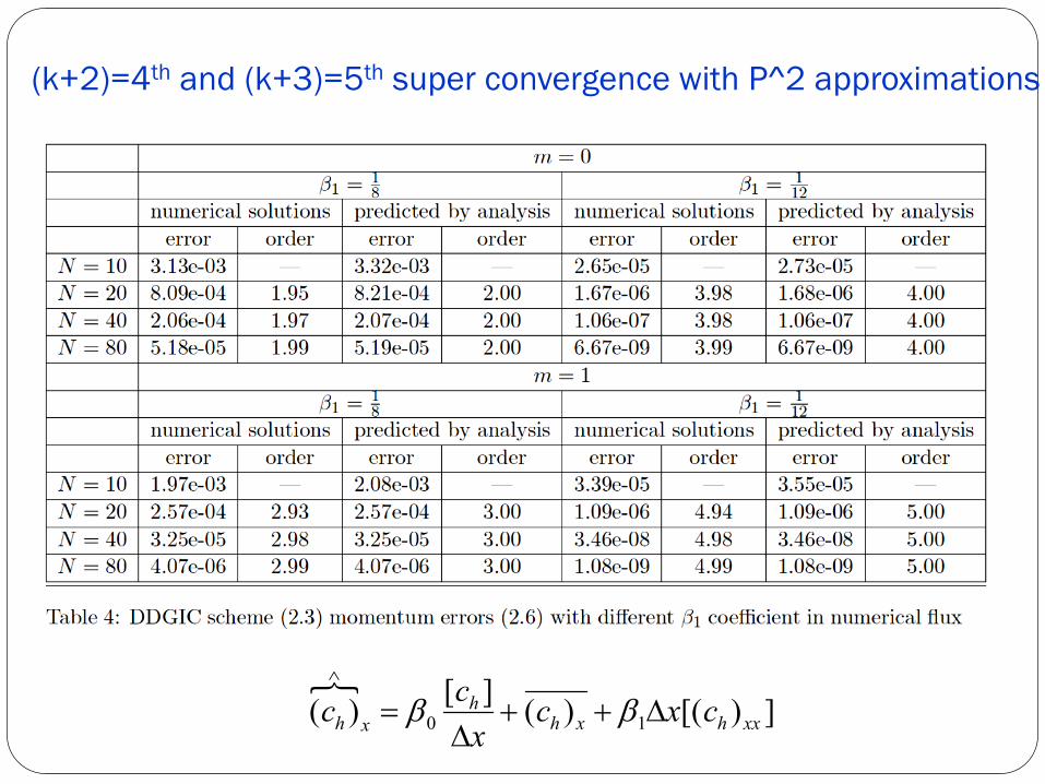
(k+2)=4th and (k+3)=5th super convergence with P^2 approximations

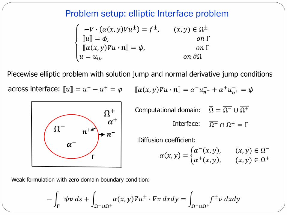
Problem setup: elliptic Interface problem

Piecewise elliptic problem with solution jump and normal derivative jump conditions

−𝛻𝛻 𝛼𝛼 𝑥𝑥, 𝑑𝑑 𝛻𝛻𝑢𝑢± = 𝑓𝑓±, (𝑥𝑥, 𝑑𝑑) ∈ Ω±

𝑢𝑢 = 𝜙𝜙, 𝑜𝑜𝑛𝑛 Γ𝛼𝛼 𝑥𝑥,𝑑𝑑 𝛻𝛻𝑢𝑢 𝒏𝒏 = 𝜓𝜓, 𝑜𝑜𝑛𝑛 Γ

𝑢𝑢 = 𝑢𝑢0, 𝑜𝑜𝑛𝑛 𝜕𝜕Ω

𝑢𝑢 = 𝑢𝑢− − 𝑢𝑢+ = 𝜑𝜑 𝛼𝛼 𝑥𝑥,𝑑𝑑 𝛻𝛻𝑢𝑢 𝒏𝒏 = 𝛼𝛼−𝑢𝑢𝒏𝒏−− + 𝛼𝛼+𝑢𝑢𝒏𝒏+− = 𝜓𝜓across interface:

Ω−Ω+

𝝘𝝘

𝜶𝜶−

𝜶𝜶+ Ω− ∩ Ω+ = ΓInterface:

Computational domain: Ω = Ω− ∪ Ω+

𝛼𝛼 𝑥𝑥,𝑑𝑑 = 𝛼𝛼− 𝑥𝑥,𝑑𝑑 , (𝑥𝑥,𝑑𝑑) ∈ Ω−

𝛼𝛼+ 𝑥𝑥,𝑑𝑑 , (𝑥𝑥,𝑑𝑑) ∈ Ω+

𝒏𝒏−𝒏𝒏+Diffusion coefficient:

−Γ𝜓𝜓𝑣𝑣 𝑑𝑑𝑠𝑠 +

Ω−∪Ω+𝛼𝛼 𝑥𝑥, 𝑑𝑑 𝛻𝛻𝑢𝑢± 𝛻𝛻𝑣𝑣 𝑑𝑑𝑥𝑥𝑑𝑑𝑑𝑑 =

Ω−∪Ω+𝑓𝑓±𝑣𝑣 𝑑𝑑𝑥𝑥𝑑𝑑𝑑𝑑

Weak formulation with zero domain boundary condition:

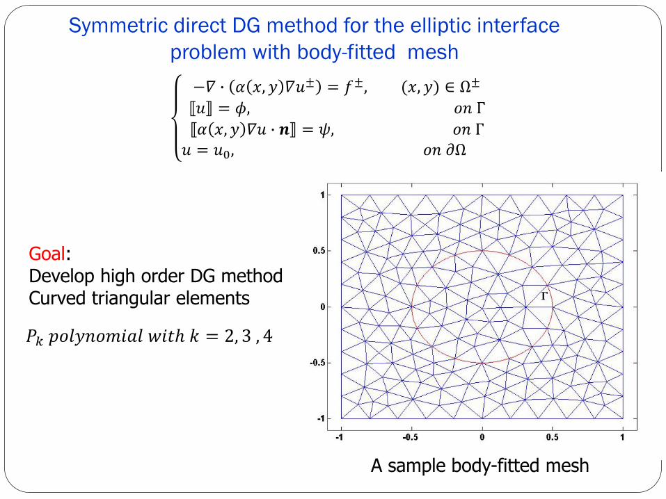
Symmetric direct DG method for the elliptic interface problem with body-fitted mesh

−𝛻𝛻 𝛼𝛼 𝑥𝑥, 𝑑𝑑 𝛻𝛻𝑢𝑢± = 𝑓𝑓±, (𝑥𝑥, 𝑑𝑑) ∈ Ω±

𝑢𝑢 = 𝜙𝜙, 𝑜𝑜𝑛𝑛 Γ𝛼𝛼 𝑥𝑥,𝑑𝑑 𝛻𝛻𝑢𝑢 𝒏𝒏 = 𝜓𝜓, 𝑜𝑜𝑛𝑛 Γ

𝑢𝑢 = 𝑢𝑢0, 𝑜𝑜𝑛𝑛 𝜕𝜕Ω

A sample body-fitted mesh

Goal: Develop high order DG methodCurved triangular elements

𝑃𝑃𝑘𝑘 𝑝𝑝𝑜𝑜𝑝𝑝𝑑𝑑𝑛𝑛𝑜𝑜𝑝𝑝𝑝𝑝𝑎𝑎𝑝𝑝 𝑤𝑤𝑝𝑝𝑤𝑤ℎ 𝑘𝑘 = 2, 3 , 4

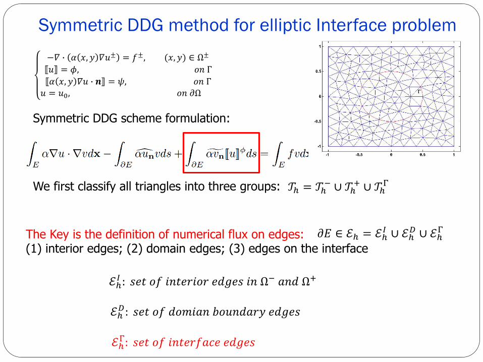
Symmetric DDG method for elliptic Interface problem

Symmetric DDG scheme formulation:

The Key is the definition of numerical flux on edges:(1) interior edges; (2) domain edges; (3) edges on the interface

𝒯𝒯ℎ = 𝒯𝒯ℎ− ∪ 𝒯𝒯ℎ+ ∪ 𝒯𝒯ℎΓWe first classify all triangles into three groups:

−𝛻𝛻 𝛼𝛼 𝑥𝑥,𝑑𝑑 𝛻𝛻𝑢𝑢± = 𝑓𝑓±, (𝑥𝑥,𝑑𝑑) ∈ Ω±

𝑢𝑢 = 𝜙𝜙, 𝑜𝑜𝑛𝑛 Γ𝛼𝛼 𝑥𝑥,𝑑𝑑 𝛻𝛻𝑢𝑢 𝒏𝒏 = 𝜓𝜓, 𝑜𝑜𝑛𝑛 Γ

𝑢𝑢 = 𝑢𝑢0, 𝑜𝑜𝑛𝑛 𝜕𝜕Ω

𝜕𝜕𝜕𝜕 ∈ ℰℎ = ℰℎ𝐼𝐼 ∪ ℰℎ𝐷𝐷 ∪ ℰℎΓ

ℰℎ𝐼𝐼 : 𝑠𝑠𝑠𝑠𝑤𝑤 𝑜𝑜𝑓𝑓 𝑝𝑝𝑛𝑛𝑤𝑤𝑠𝑠𝑖𝑖𝑝𝑝𝑜𝑜𝑖𝑖 𝑠𝑠𝑑𝑑𝑒𝑒𝑠𝑠𝑠𝑠 𝑝𝑝𝑛𝑛 Ω− 𝑎𝑎𝑛𝑛𝑑𝑑 Ω+

ℰℎ𝐷𝐷: 𝑠𝑠𝑠𝑠𝑤𝑤 𝑜𝑜𝑓𝑓 𝑑𝑑𝑜𝑜𝑝𝑝𝑝𝑝𝑎𝑎𝑛𝑛 𝑏𝑏𝑜𝑜𝑢𝑢𝑛𝑛𝑑𝑑𝑎𝑎𝑖𝑖𝑑𝑑 𝑠𝑠𝑑𝑑𝑒𝑒𝑠𝑠𝑠𝑠

ℰℎΓ: 𝑠𝑠𝑠𝑠𝑤𝑤 𝑜𝑜𝑓𝑓 𝑝𝑝𝑛𝑛𝑤𝑤𝑠𝑠𝑖𝑖𝑓𝑓𝑎𝑎𝑐𝑐𝑠𝑠 𝑠𝑠𝑑𝑑𝑒𝑒𝑠𝑠𝑠𝑠

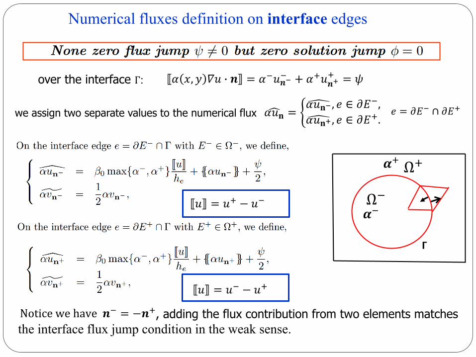
Numerical fluxes definition on interface edges

Notice we have 𝒏𝒏− = −𝒏𝒏+, adding the flux contribution from two elements matchesthe interface flux jump condition in the weak sense.

𝛼𝛼 𝑥𝑥,𝑑𝑑 𝛻𝛻𝑢𝑢 𝒏𝒏 = 𝛼𝛼−𝑢𝑢𝒏𝒏−− + 𝛼𝛼+𝑢𝑢𝒏𝒏++ = 𝜓𝜓over the interface Γ:

𝛼𝛼𝑢𝑢𝐧𝐧 = 𝛼𝛼𝑢𝑢𝐧𝐧− , 𝑠𝑠 ∈ 𝜕𝜕𝜕𝜕−,𝛼𝛼𝑢𝑢𝐧𝐧+ , 𝑠𝑠 ∈ 𝜕𝜕𝜕𝜕+.we assign two separate values to the numerical flux 𝑠𝑠 = 𝜕𝜕𝜕𝜕− ∩ 𝜕𝜕𝜕𝜕+

𝑢𝑢 = 𝑢𝑢+ − 𝑢𝑢−

𝑢𝑢 = 𝑢𝑢− − 𝑢𝑢+

Ω−Ω+

𝝘𝝘

𝜶𝜶−

𝜶𝜶+

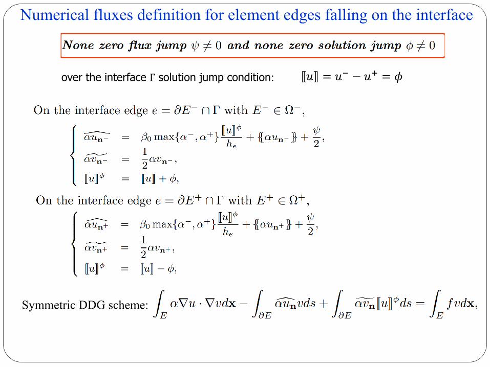
Numerical fluxes definition for element edges falling on the interface

Symmetric DDG scheme:

over the interface Γ solution jump condition: 𝑢𝑢 = 𝑢𝑢− − 𝑢𝑢+ = 𝜙𝜙

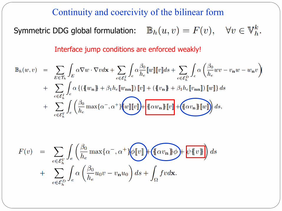
Continuity and coercivity of the bilinear form

Symmetric DDG global formulation:

Interface jump conditions are enforced weakly!

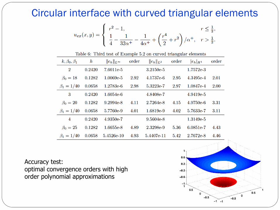
Circular interface with curved triangular elements

Accuracy test:optimal convergence orders with high order polynomial approximations

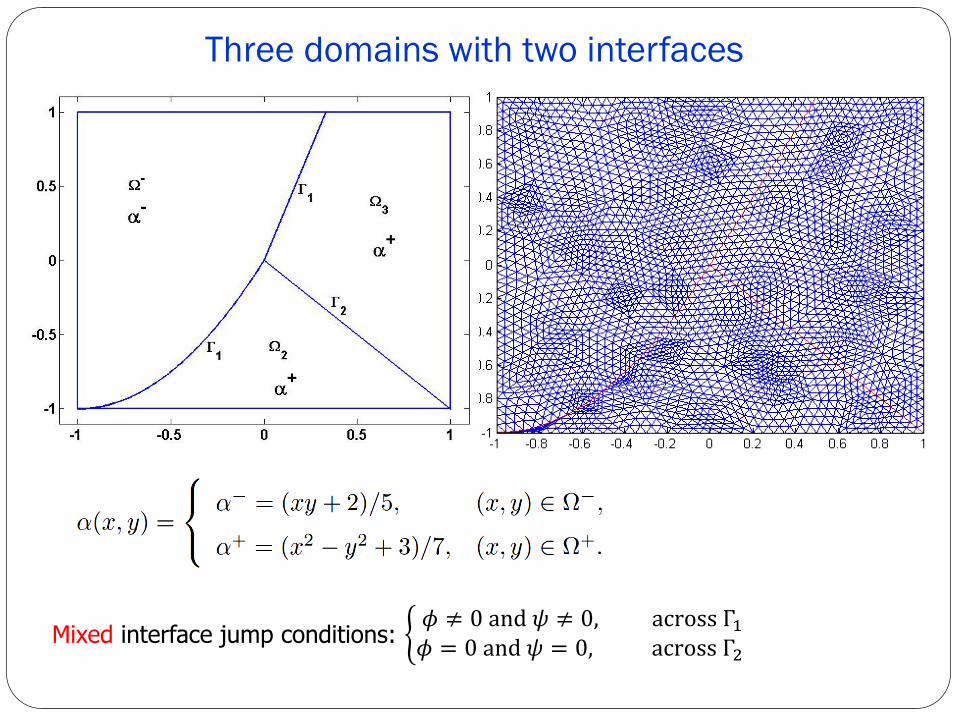
Three domains with two interfaces

Mixed interface jump conditions: 𝜙𝜙 ≠ 0 and 𝜓𝜓 ≠ 0, across Γ1𝜙𝜙 = 0 and 𝜓𝜓 = 0, across Γ2

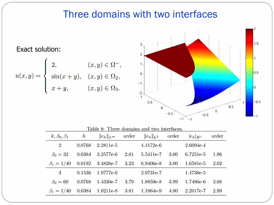
Exact solution:

Three domains with two interfaces

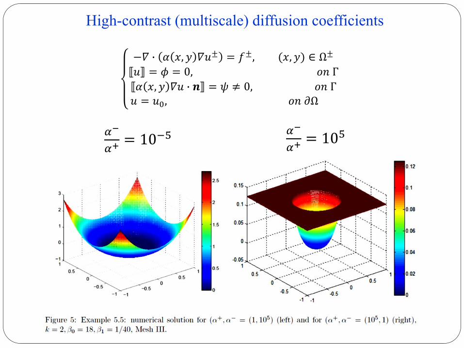
High-contrast (multiscale) diffusion coefficients

𝛼𝛼−

𝛼𝛼+= 10−5 𝛼𝛼−

𝛼𝛼+= 105

−𝛻𝛻 𝛼𝛼 𝑥𝑥,𝑑𝑑 𝛻𝛻𝑢𝑢± = 𝑓𝑓±, (𝑥𝑥,𝑑𝑑) ∈ Ω±

𝑢𝑢 = 𝜙𝜙 = 0, 𝑜𝑜𝑛𝑛 Γ𝛼𝛼 𝑥𝑥,𝑑𝑑 𝛻𝛻𝑢𝑢 𝒏𝒏 = 𝜓𝜓 ≠ 0, 𝑜𝑜𝑛𝑛 Γ𝑢𝑢 = 𝑢𝑢0, 𝑜𝑜𝑛𝑛 𝜕𝜕Ω

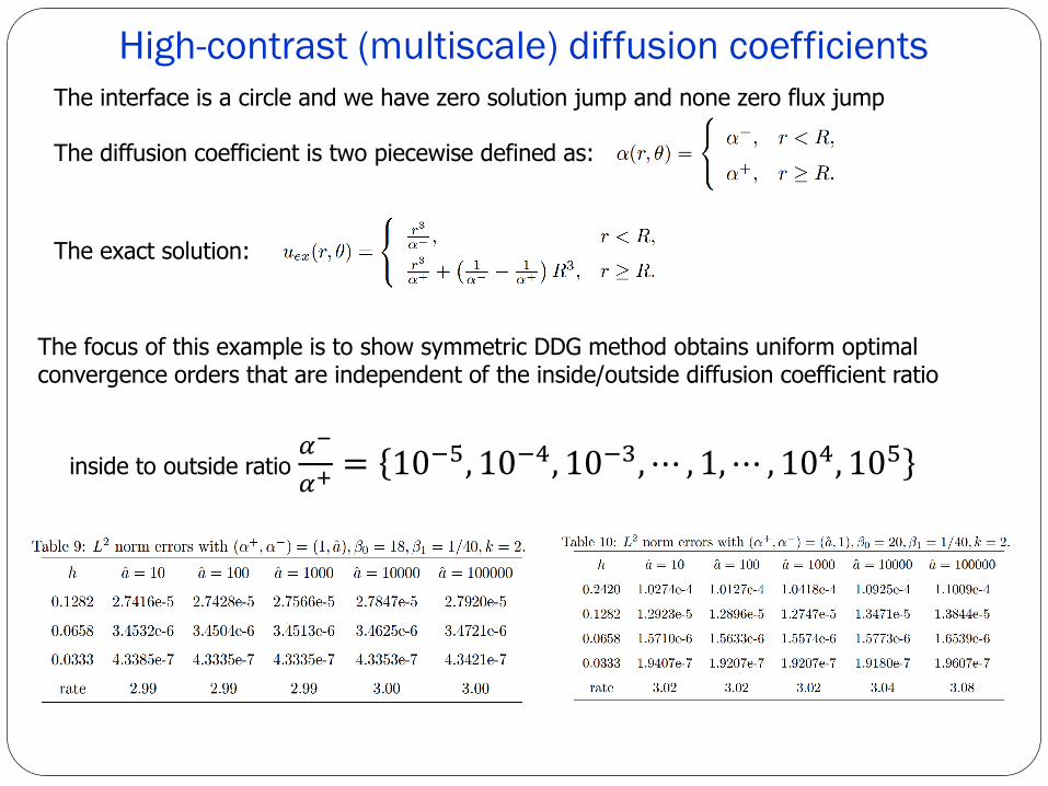
High-contrast (multiscale) diffusion coefficientsThe interface is a circle and we have zero solution jump and none zero flux jump

The diffusion coefficient is two piecewise defined as:

The exact solution:

The focus of this example is to show symmetric DDG method obtains uniform optimal convergence orders that are independent of the inside/outside diffusion coefficient ratio

inside to outside ratio 𝛼𝛼−

𝛼𝛼+= 10−5, 10−4, 10−3,⋯ , 1,⋯ , 104, 105

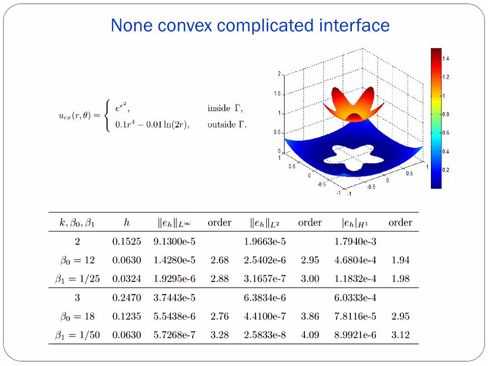
None convex complicated interface

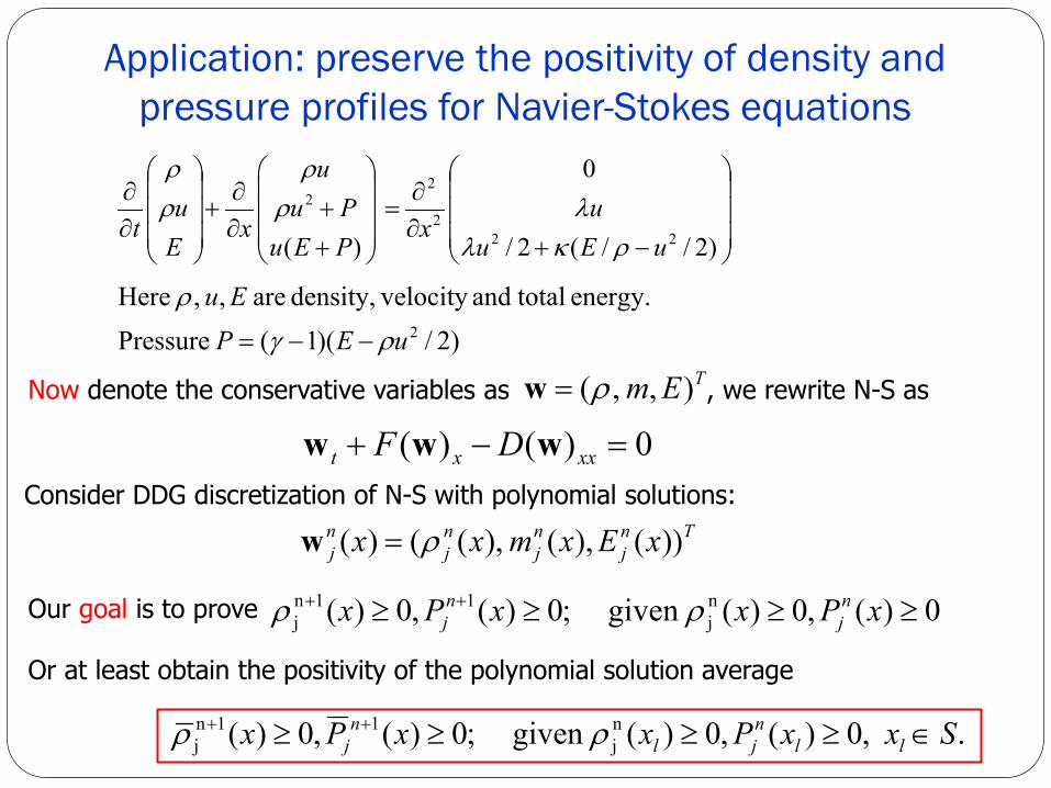
Application: preserve the positivity of density and pressure profiles for Navier-Stokes equations

)2//(2/

0

)(

222

22

−+∂∂

=

++

∂∂

+

∂∂

uEuu

xPEuPu

u

xEu

tρκλ

λρρ

ρρ

)2/)(1( Pressure energy. totaland velocity density, are , , Here

2uEPEu

ργ

ρ

−−=

Now denote the conservative variables as , we rewrite N-S asTEm ), ,(ρ=w

0)()( =−+ xxxt DF www

Our goal is to prove 0)(,0)(given ;0)(,0)( nj

11nj ≥≥≥≥ ++ xPxxPx n

jnj ρρ

Or at least obtain the positivity of the polynomial solution average

. ,0)(,0)(given ;0)(,0)( nj

11nj SxxPxxPx ll

njl

nj ∈≥≥≥≥ ++ ρρ

Consider DDG discretization of N-S with polynomial solutions:Tn

jnj

nj

nj xExmxx ))(),( ,)(()( ρ=w

Conclusions Introduce the direct discontinuous Galerkin method

Show the advantages of DDG method Maximum-principle-satisfying or positivity-preserving Super convergence phenomena Elliptic interface problems

Current and future work DDG methods for strong nonlinear diffusion (compressible N-S

equations) Meshes being cut by the curved interface

Stokes interface problems

Thanks for your attention!