Embed Size (px)
Citation preview
ALTERNATING EVOLUTION DISCONTINUOUS GALERKIN METHODS FOR
HAMILTON-JACOBI EQUATIONS
HAILIANG LIU AND MICHAEL POLLACK
Abstract. In this work, we propose a high resolution Alternating Evolution Discontinuous Galerkin
(AEDG) method to solve Hamilton-Jacobi equations. The construction of the AEDG method is based
on an alternating evolution system of the Hamilton-Jacobi equation, following the previous work [H.Liu, M. Pollack and H. Saran, SIAM J. Sci. Comput. 35(1), (2013) 122–149] on AE schemes for
Hamilton-Jacobi equations. A semi-discrete AEDG scheme derives directly from a sampling of this
system on alternating grids. Higher order accuracy is achieved by a combination of high-order poly-nomial approximation near each grid and a time discretization with matching accuracy. The AEDG
methods have the advantage of easy formulation and implementation, and efficient computation of thesolution. For the linear equation, we prove the L2 stability of the method. Numerical experiments for
a set of Hamilton-Jacobi equations are presented to demonstrate both accuracy and capacity of these
AEDG schemes.
Contents
1. Introduction 12. Alternating evolution DG methods 42.1. Semi-discrete AEDG formulation 42.2. Discrete ODEs 52.3. Troubled cell detection and limiters 62.4. Time discretization 73. Stability analysis 74. The multi-dimensional case 85. Numerical tests 106. Concluding remarks 16Acknowledgments 17References 17
1. Introduction
In this paper, we develop a new alternating evolution discontinuous Galerkin (AEDG) method tosolve time-dependent Hamilton-Jacobi (H-J) equations. We describe the designing principle of ourAEDG scheme through the following form:
(1.1) φt +H(x, φ,∇xφ) = 0, φ(x, 0) = φ0(x), x ∈ Rd, t > 0.
Here, d is the space dimension, the unknown φ is scalar, and H : Rd → R1 is a nonlinear Hamiltonian.The Hamilton-Jacobi equation arises in many applications ranging from geometrical optics to differentialgames. These nonlinear equations typically develop discontinuous derivatives even with smooth initialconditions, the solutions of which are non-unique. In this paper, we are only interested in the viscositysolution [11, 12, 34], which is the physically relevant solution in some important applications.
Date: June 27, 2013.
1991 Mathematics Subject Classification. 65M06, 65M12, 35L02.Key words and phrases. Alternating evolution, Hamilton-Jacobi equations, viscosity solution.
1
2 HAILIANG LIU AND MICHAEL POLLACK
The difficulty encountered for the satisfactory approximation of the exact solutions of these equationslies in the presence of discontinuities in the solution derivatives. An important class of finite differencemethods for computing the viscosity solution is the class of monotone schemes introduced by Crandall-Lions [13]. Unfortunately, monotone schemes are at most first-order accurate. The need for devisingmore accurate numerical methods for Hamilton-Jacobi equations has prompted the abundant researchin this area in the last two decades, including essentially non-oscillatory (ENO) or weighted ENO(WENO) finite difference schemes, see e.g., [15, 17, 21, 27, 28, 33, 36], and Central or Central-Upwindfinite difference schemes, see e.g., [2, 3, 4, 19, 20, 22, 23], as well as discontinuous Galerkin methods[5, 16, 25, 35].
The preliminary goal of this paper is to design high order discontinuous Galerkin methods forHamilton-Jacobi equations by following the alternating evolution framework introduced in [24] for hy-perbolic conservation laws; see local AE schemes developed by Saran and Liu [30], see also [1]. The highresolution finite difference scheme under this AE framework was further developed for Hamilton-Jacobiequations in [31]. In such a framework, the general setting is to refine the original PDE by an alternatingevolution (AE) system which involves two representatives: {u, v}. To update u, terms involving spatialderivatives are replaced by v’s derivatives and augmented by an additional relaxation term (v − u)/ε,which serves to communicate the two representatives. The AE system for scalar hyperbolic conservationlaws was shown in [24] to be capable of capturing the exact solution when initially both representativesare chosen as the given initial data. Such a feature allows for a sampling of two representatives overalternating grids. Using this alternating system as a ‘building base’, we apply standard approximationtechniques to the AE system.
For Hamilton-Jacobi equations, we consider the following alternating evolution system
ut +H(x, u,∇xv) =1
ε(v − u),
vt +H(x, v,∇xu) =1
ε(u− v).
Here, ε > 0 is a scale parameter of user’s choice. At t = 0, we take the initial data
u0(x) = v0(x) = φ0(x).
We sample the above system over alternating grids when performing the spatial discretization, leadingto a class of high order semi-discrete AEDG schemes.
The semi-discrete scheme thus obtained has the form
d
dt
∫Iα
Φηdx+
∫Iα
H(x,Φ,∇xΦSN )ηdx+ λ[Φ]η|xα +1
ε
∫Iα
Φηdx =1
ε
∫Iα
ΦSNηdx,
where λ = Hp(x,Φ(x),∇xΦ), and ΦSN are polynomial elements sampled from neighboring cells Iα±ej .The scale parameter ε and the time step size ∆t are chosen to stabilize the time discretization. In theone-dimensional case with H = βp, the semi-discrete AEDG scheme of first order becomes
d
dtΦα + β
(Φα+1 − Φα−1
2∆x
)=
1
2ε(Φα+1 − 2Φα + Φα−1),
which, using Euler-forward with ε = ∆t, reduces to the celebrated Lax-Friedrichs scheme
Φn+1α =
1
2(Φnα+1 + Φnα−1)− εβ
(Φnα+1 − Φnα−1
2∆x
).
We recall that the success of finite difference schemes for Hamilton-Jacobi equations is due to twofactors: the local enforcement of the equation in question and the non-oscillatory piecewise polynomialinterpolation from evolved grid values. The difference in the AE schemes proposed in [31] and theexisting finite difference schemes lies in the local enforcement. The ENO/WENO type schemes ([17,21, 27, 28, 32, 33, 36]) are based mainly on some local refinement of H-J equations by
(1.2) φt + H(x, φ+x , φ
−x ) = 0,
AEDG SCHEMES FOR HAMILTON JACOBI EQUATIONS 3
where H is the numerical Hamiltonian which needs to be carefully chosen to ensure that the viscositysolution is captured when φx becomes discontinuous. In comparison, the central type schemes ( [2, 3,4, 19, 20, 22, 23]) choose to evolve the constructed polynomials in smooth regions such that the Taylorexpansion may be used in the scheme derivation.
Finite difference methods are quite efficient for Cartesian meshes. However, on unstructured meshes,the scheme is quite complicated. Alternatively, the discontinuous Galerkin (DG) method, originallydevised to solve first order partial differential equations such as conservation laws [6, 7, 8, 9, 10, 29], hasthe advantage of flexibility for arbitrarily unstructured meshes, and with the ability to easily achievearbitrary order of accuracy. However, some new difficulties occur when the existing ideas with finitedifference methods are applied toward some discontinuous Galerkin discretization. One main difficultycomes from the non-conservative form of the equation, which precludes the use of integration by partsto establish the cell to cell communication via numerical fluxes as usually done with the DG methods forhyperbolic conservation laws. In spite of this difficulty, some progress has been made. In [16], Hu andShu proposed a discontinuous Galerkin method to solve the Hamilton-Jacobi equation φt+H(∇xφ) = 0.They use the fact that the derivative of the solution φ satisfies a conservation law system, and applythe usual discontinuous Galerkin method on this system to advance the derivatives of φ. The solutionφ itself is then recovered from these derivatives by a least square procedure for multi-dimensional casesand with an independent evolution of the cell averages of φ. However, in the multi-dimensional case,a single equation of φ is converted to a system of w = ∇xφ, which is only weakly hyperbolic at somepoints. Also, the resulting algorithm appears indirect and complicated. This motivates the developmentof another DG method in [5] for directly solving H-J equations; for nonlinear convex Hamiltonians, theirnumerical experiments demonstrate that the method is stable and accurate, however, entropy correctionis needed near the kink formation in some cases. In [35], Yan and Osher apply the LDG discretizationto (1.2) by introducing two additional variables p1 = φ+
x and p2 = φ−x and then apply the usualdiscontinuous Galerkin method to advance (φ, p1, p2) all together in the one-dimensional case, with anextension to the two dimensional case.
In [25], Li and Yakovlev proposed a central discontinuous Galerkin method that directly solvesthe Hamilton-Jacobi equations using two polynomial representatives solved on two sets of overlappingmeshes [26]. The AEDG scheme proposed in this paper only has one polynomial representative asso-ciated with each grid point, even in multi-dimensional case. The scheme that we design here is alsodifferent in that it is based on alternatively sampling the AE system of the Hamilton-Jacobi equationwith spatial accuracy enhanced by interlaced polynomials. However, the AEDG is also similar to thecentral DG scheme in the sense that neighboring polynomials in the AEDG (the other representativepolynomials in the central DG) are used whenever a calculation of the Hamiltonian is needed. Forthe one dimensional Hamiltonian H(x, φ, φx), the two schemes are almost equivalent when rescalingthe mesh size ∆x to 2∆x, except that in the AEDG scheme the neighboring polynomials are usedto compute only the solution gradient φx, while the central DG method uses the other representativepolynomials to compute the entire H(x, φ, φx). The main advantage of the AEDG scheme is that inthe multi-dimensional case, the alternating evolution framework results in easy formulation of the com-putation of the Hamiltonian. For example, in the two dimensional case, AEDG evaluates the gradientusing the closest polynomials.
It should be noted that even though our AEDG schemes are derived based on sampling the alternatingevolution system, we do not solve the system directly. The AE system simply provides a systematic wayfor developing numerical schemes of both semi-discrete and fully discrete form for the original problem,instead of as an approximation system at the continuous level.
The article is organized as follows: in section 2, we formulate the AEDG method for one dimensionalHamilton-Jacobi equations. We also discuss the use of kink detector, and reconstruction of polynomialelements to make the approximation less oscillatory, so that the computed solution is the viscositysolution as desired. We then give a rigorous proof of L2 stability by the AEDG method for H = αp insection 3. Extensions to the multi-D case is given in section 4. In section 5, we show numerical results,
4 HAILIANG LIU AND MICHAEL POLLACK
which includes both one and two dimensional problems. The results illustrate accuracy, efficiency, andhigh resolution near kinks. The last section 6 ends this paper with our concluding remarks.
2. Alternating evolution DG methods
Our numerical schemes for H-J equations consist of a semi-discrete formulation based on sampling ofthe AE system on alternating grids and a fully discrete version by using an appropriate Runge-Kuttasolver.
To illustrate, we start with the one-dimensional Hamilton-Jacobi equation of the form
φt +H(x, φ, φx) = 0.
The ‘building base’ is the following AE system
ut +H(x, u, vx) =1
ε(v − u),(2.1)
vt +H(x, v, ux) =1
ε(u− v).(2.2)
2.1. Semi-discrete AEDG formulation. We develop an AE discontinuous Galerkin (AEDG) methodfor the H-J equation subject to initial data φ0(x). We divide the spatial domain to form a uniform grid,and let {xj} be the grid point, with ∆x = xj+1 − xj . We denote Ij = (xj−1, xj+1) for j = 2, . . . , N − 1with I1 = (x1, x2) and IN = (xN−1, xN ). Centered at each grid {xj}, the numerical approximation is apolynomial Φ|Ij = Φj(x) ∈ P k, where P k denotes a linear space of all polynomials of degree at most k:
P k := {p | p(x)|Ij =∑
0≤i≤k
ai(x− xj)i, ai ∈ R}.
Note dim(P k) = k + 1. We denote v(x±) = limε→0± v(x + ε), and v±j = v(x±j ). The jump at xj is
[v]j = v(x+j ) − v(x−j ), and the average {v}j = 1
2 (v+j + v−j ). Integrating the AE system (2.1) over Ij
against the test function η ∈ P k(Ij), we obtain the semi-discrete AEDG scheme∫Ij
(∂tΦj +H(x,Φj , ∂xΦSNj ))ηdx+ λ[ΦSNj ]∣∣∣xjη(xj) = 1
ε
(∫Ij
ΦSNj ηdx−∫Ij
Φjηdx),(2.3)
where λ = Hp(xj ,Φj(xj), ∂xΦj(xj)) and ΦSNj are sampled from neighboring polynomials Φj±1 in thefollowing way:∫
Ij
H(x,Φj , ∂xΦSNj )ηdx =
∫ xj
xj−1
H(x,Φj , ∂xΦj−1)ηdx+
∫ xj+1
xj
H(x,Φj , ∂xΦj+1)ηdx,∫Ij
ΦSNj ηdx =
∫ xj
xj−1
Φj−1ηdx+
∫ xj+1
xj
Φj+1ηdx,
[ΦSNj ]∣∣∣xj
= Φj+1(x+j )− Φj−1(x−j ).
To update each grid-centered polynomial element Φ, we write the compact form of the semi-discretescheme
d
dt
∫Ij
Φjηdx = L[Φj ; ΦSNj , η](t),(2.4)
where
L[Φj ; Φj±1, η](t) =1
ε
∫Ij
(ΦSNj − Φj)ηdx−∫Ij
H(x,Φj , ∂xΦSNj
)ηdx− λ[ΦSNj ]|xjη(xj).(2.5)
AEDG SCHEMES FOR HAMILTON JACOBI EQUATIONS 5
For cells near the boundary we treat with care. For a computational domain [a, b] with x1 = a, xN = band ∆x = (b− a)/(N − 1), the two equations near boundary may be given as∫ x2
x1
(∂tΦ1 +H(x,Φ1, ∂xΦ2))ηdx+λ
2[Φ]|x1
η(x1) =1
ε
∫ x2
x1
(Φ2 − Φ1)ηdx,(2.6) ∫ xN
xN−1
(∂tΦN +H(x,ΦN , ∂xΦN−1))ηdx+λ
2[Φ]|xN η(xN ) =
1
ε
∫ xN
xN−1
(ΦN−1 − ΦN )ηdx.(2.7)
At the left boundary, η ∈ P k(x1, x2), and on the right boundary, η ∈ P k(xN−1, xN ), so that the lengthof the interval is ∆x instead of 2∆x.
If the flow is incoming at x = a, one has to impose a boundary condition φ(a, t) = g1(t). As aresult, one is required to modify (2.6) by changing [Φ] to Φ2(x+
1 ) − g1(t); for the outflow case, onemay take [Φ] = 0 in (2.6). Similarly, at x = b, the inflow boundary condition φ(b, t) = g2(t) can beincorporated in (2.7) by replacing [Φ] by g2(t) − ΦN−1(x−N , t); and for outgoing flow, replacing [Φ] by0. The determination of the inflow or outflow of the boundary condition may be obtained by checkingthe sign of the characteristic speed ∂xH(x, φ, p). In the case of periodic boundary conditions, [Φ] canbe computed as Φ2(x+
1 )− ΦN−1(x−N ) at x = x1, xN , and ΦN (x) is regarded to be identical to Φ1(x).The fully discrete scheme follows from applying an appropriate Runge-Kutta solver to (2.4). We
summarize the algorithm as follows.
Algorithm:
1. Initialization: in any cell Ij , compute the initial data by the local L2−projection
(2.8)
∫Ij
(Φ0 − φ0)ηdx = 0, η ∈ P k(Ij).
2. Alternating evaluation : take polynomials Φj±1(x) = Φ|Ij±1 , and then sample in Ij to getL[Φj ; Φj±1, η] as defined in (2.5).
3. Evolution: obtain Φn+1 from Φn by some Runge-Kutta type procedure to solve the ODE system(2.4).
In the AEDG schemes, ε is chosen such that the stability condition,
∆t ≤ ε ≤ Q ∆x
max |Hp(x, p)|,
is satisfied. The choice of Q depends on the order of the scheme, similar to that used in the AE finitedifference scheme introduced in [31].
2.2. Discrete ODEs. We now present AE schemes with polynomial elements of degree k for H-Jequations.
Let {φl(ξ)}k+1l=1 be the basis in the master domain [−1, 1], then in each cell Ij we can express
Φj(x) =
k+1∑l=1
aljφl(ξ) =: φ>(ξ)aj , ξ =x− xj
∆x,
then
Φj±1(x) =
k+1∑l=1
alj±1φl(ξ ∓ 1) = φ>(ξ ∓ 1)aj±1.
A simple calculation of (2.3) gives
(2.9) Maj = −1
εMaj +
1
εLj ,
where
M = h
∫ 1
−1
φ(ξ)φ>(ξ)dξ, Lj = C−aj−1 + C+aj+1 − εhHj
6 HAILIANG LIU AND MICHAEL POLLACK
with
C− = h
∫ 0
−1
φ(ξ + 1)φ>(ξ)dξ + ελφ(0)φ>(1),
C+ = h
∫ 1
0
φ(ξ − 1)φ>(ξ)dξ − ελφ(0)φ>(−1),
Hj =
∫ 0
−1
φ(ξ)H(xj + hξ, φ>(ξ)aj , h−1∂ξφ
>(ξ + 1)aj−1)dξ
+
∫ 1
0
φ(ξ)H(xj + hξ, φ>(ξ)aj , h−1∂ξφ
>(ξ − 1)aj+1)dξ.
The Hamiltonian H is generally nonlinear, some quadrature rule must be applied to evaluate Hj . Theparameter λ is used to ensure the stability. The following two options are acceptable:
λ = λj = Hp(xj ,Φj(xj),1
2(∂xΦj+1 + ∂xΦj−1)(xj))
or
λ = Hp(xj ,Φj(xj), ∂xΦj(xj)).
2.3. Troubled cell detection and limiters. It is known that near singularities one may need toimpose some limiters so that the proposed scheme can capture the viscosity solution. To determinewhich cells are troubled cells and require an application of a limiter, we use a strategy that is based ona strong superconvergence as in [18]. We construct the troubled cell detector in one dimensional case:
Ij =|∂xφj−1(x−j )− ∂xφj+1(x+
j )|hk−12 ||φ||L2(Ij)
.
The order of the numerator can be determined by the continuity of φx at the interface x = xj ,
|∂xφj−1(x−j )− ∂xφj+1(x+j )| =
{O(hk), if φx is smooth,
O(1), if φx is discontinuous,
so that
Ij =
{O(h
k2 ), if φx is smooth,
O(h−k2 ), if φx is discontinuous,
for k ≥ 1. Then, Ij → 0 as h → 0 in smooth regions and Ij → ∞ as h → 0 in nonsmooth regions.So, if Ij > 1, then φx is discontinuous and the cell Ij is identified as a troubled cell. A limiter is thenapplied to that cell to obtain φnew
j . If Ij < 1, then φx is continuous so that φnewj = φj .
In order to capture the viscosity solution, nonlinear limiters are applied (see [25]) to the detectedtroubled cells. For k = 1, φj is written as
φj = a1j + a2
j
(x− xj
∆x
).
In order to update the a2j term, we consider two new candidates for the slope of φj ,
sLj = a1j − a1
j−1, sRj = a1j+1 − a1
j .
We then compute
a2j = MM
(a2j , s
Lj , s
Rj
).
Here MM denotes the Min-Mod nonlinear limiter
MM{b1, b2, · · · } =
minj{bj} if bj > 0, ∀j,maxj{bj} if bj < 0, ∀j,0 otherwise.
AEDG SCHEMES FOR HAMILTON JACOBI EQUATIONS 7
If∣∣a2j − a2
j
∣∣ ≤ ε for small ε, then no change is needed. Otherwise, a2j = a2
j .
For k = 2,
φj = a1j + a2
j
(x− xj
∆x
)+ a3
j
(x− xj
∆x
)2
.
The application of the limiter to a2j is the same as in the k = 1 case. Once the a2
j terms have
been updated, the a3j terms are updated in a similar fashion, but for the polynomial ∆x∂xφj = a2
j +
2a3j
(x−xj∆x
). The second derivative approximations can be computed as
(s′j)L = a2
j − a2j−1, (s′j)
R = a2j+1 − a2
j .
We then compute
a3j = MM
(2a3j , (s
′j)L, (s′j)
R).
If∣∣a3j − a3
j
∣∣ ≤ ε for small ε, then no change is needed. Otherwise, a3j = a3
j/2.
2.4. Time discretization. We now turn to time discretization of (2.9), following [28]. Let {tn}, n =0, 1, . . . ,K be a uniform partition of the time interval [0, T ]. Let Φ0 = Pφ0 be the piecewise L2
projection of φ0(x) defined in (2.8), and A = [a1, · · · , aN ]>, then
At = G(A).
We use the third order explicit SSP Runge-Kutta method [14] for time discretization. In details, let An
be the solution at time level n,
(2.10)
A(1) = An + ∆tG(An),
A(2) =3
4A(0) +
1
4
(A(1) + ∆tG(A(1))
),
An+1 =1
3A(0) +
2
3
(A(2) + ∆tG(A(2))
).
3. Stability analysis
In this section we show that the semi-discrete AEDG scheme is L2stable for linear Hamiltonian. Inparticular, when H = αp, α = const., we have the following.
Theorem 3.1. Let Φ be computed from the AEDG scheme (2.4) for the Hamilton-Jacobi equationφt +H(φx) = 0 with linear Hamiltonian H(p) = αp and periodic boundary conditions. Then
d
dt
N−1∑j=1
∫ xj+1
xj
Φ2j+1 + Φ2
j
2dx
= −1
ε
N−1∑j=1
∫ xj+1
xj
(Φj+1 − Φj)2dx.
Proof. Taking η = Φ2i =: u in (2.4) for j = 2i, and η = Φ2i+1 =: v in (2.4) for j = 2i+ 1, respectively,it gives
d
dt
∫I2i
u2
2dx+
∫I2i
H(x, u, vx)udx+ λ[v]u|x2i=
1
ε
(∫I2i
uvdx−∫I2i
u2dx
),
d
dt
∫I2i+1
v2
2dx+
∫I2i+1
H(x, v, ux)vdx+ λ[u]v|x2i+1=
1
ε
(∫I2i+1
uvdx−∫I2i+1
v2dx
).
Note that
[a, b] = ∪N/2−1i=1 I2i + [xN−1, xN ] = [x1, x2] + ∪N/2−1
i=1 I2i+1,
8 HAILIANG LIU AND MICHAEL POLLACK
we sum over all index and use (2.6)-(2.7) to obtain
d
dt
∫ b
a
u2
2dx+
N/2−1∑i=1
∫I2i
+
∫ xN
xN−1
H(x, u, vx)udx+
N/2−1∑i=1
λ[v]u|x2i+
1
2λ[v]u|xN =
1
ε
∫ b
a
(uv − u2)dx,
d
dt
∫ b
a
v2
2dx+
∫ x2
x1
+
N/2−1∑i=1
∫I2i+1
H(x, v, ux)vdx+1
2λ[u]v|x1
+
N/2−1∑i=1
λ[u]v|x2i+1=
1
ε
∫ b
a
(uv − v2)dx.
Adding these two relations up, we obtain
d
dt
∫ b
a
u2 + v2
2dx+ J1 + J2 = −1
ε
∫ b
a
(u− v)2dx,
where for H(p) = αp all other terms in J1 and J2 are expressed as follows:
J1 =
N/2∑i=1
∫ x2i
x2i−1
+
N/2−1∑i=1
∫ x2i+1
x2i
[H(x, u, vx)u+H(x, v, ux)v]dx
= −α
N/2−1∑i=1
[u]v|x2i+1+
N/2∑i=1
[v]u|x2i
− αΦ2(x+1 )Φ1(x1) + αΦN (xN )ΦN−1(x−N ).
and
J2 = λ
N/2−1∑i=1
[u]v|x2i+1 +
N/2∑i=1
[v]u|x2i
+λ
2(Φ1(x1) + ΦN (xN ))(Φ2(x+
1 )− ΦN−1(x−N )).
Using the periodic boundary condition Φ1(x1) = ΦN (xN ), we have
J1 + J2 = 0
when λ = α. �
4. The multi-dimensional case
By similar procedures we can construct AEDG schemes for multi-dimensional H-J equations:
φt +H(x, φ,∇xφ) = 0, x := (x1, · · · , xd) ∈ Rd.We start with the AE formulation
(4.1) ut +1
εu =
1
εv −H(x, u,∇xv).
Let {xα} be distributed grids in Rd. Consider Iα be a hypercube centered at xα with vertices at xα±1
where the number of vertices is 2d.Centered at each grid {xα}, the numerical approximation is a polynomial Φ|Iα = Φα(x) ∈ Pr, where
Pr denotes a linear space of all polynomials of degree at most r in all xi:
Pr := {p | p(x)|Iα =∑
0≤βi≤r
aβ(x− xα)β , 1 ≤ i ≤ d, aβ ∈ R}.
Note dim(Pr) = (r + 1)d. Sampling the AE system (4.1) in Iα, we obtain the semi-discrete AEDGscheme ∫
Iα(∂tΦα +H(x,Φα,∇xΦSNα ))ηdx+ 1
ε
∫Iα
Φαηdx = 1ε
∫Iα
ΦSNα ηdx−B,(4.2)
B =∑dj=1
∫IαHj(x,Φα,∇Φα)[Φ]η(x)δ(xj − xjαj )dx,(4.3)
where ΦSNα are sampled from neighboring polynomials, and Hj = ∂pjH(x, z, p). The choice of ΦSNα isnot unique, and we shall take
ΦSNα ∈ span{Φα±ej}dj=1.
AEDG SCHEMES FOR HAMILTON JACOBI EQUATIONS 9
In the two dimensional case with α = (i, j), the terms involving neighboring polynomials are as follows:∫ xi+1
xi−1
∫ yj+1
yj−1
H(x, y,Φ, ∂xΦSN , ∂yΦSN )ηdydx =
∫ xi+1
xi
∫ yj+1
yj
H(x, y,Φi,j , ∂xΦi+1,j , ∂yΦi,j+1)η(x, y)dydx
+
∫ xi+1
xi
∫ yj
yj−1
H(x, y,Φi,j , ∂xΦi+1,j , ∂yΦi,j−1)η(x, y)dydx
+
∫ xi
xi−1
∫ yj+1
yj
H(x, y,Φi,j , ∂xΦi−1,j , ∂yΦi,j+1)η(x, y)dydx
+
∫ xi
xi−1
∫ yj
yj−1
H(x, y,Φi,j , ∂xΦi−1,j , ∂yΦi,j−1)η(x, y)dydx.
An average of two neighboring polynomials Φi±1,j and Φi,j±1 will be used to evaluate∫Iα
ΦSNηdx, thatis ∫
Iα
ΦSNηdx =1
2
∫ xi+1
xi
∫ yj+1
yj
(Φi+1,j + Φi,j+1)η(x, y)dydx
+1
2
∫ xi+1
xi
∫ yj
yj−1
(Φi+1,j + Φi,j−1)η(x, y)dydx
+1
2
∫ xi
xi−1
∫ yj+1
yj
(Φi−1,j + Φi,j+1)η(x, y)dydx
+1
2
∫ xi
xi−1
∫ yj
yj−1
(Φi−1,j + Φi,j−1)η(x, y)dydx.
The B term in (4.3) can then be computed as
B =
∫ yj+1
yj−1
H1 (x, y,Φi,j , ∂xΦi,j , ∂yΦi,j)(Φi+1,j(x
+i , y)− Φi−1,j(x
−i , y)
)η(xi, y)dy
+
∫ xi+1
xi−1
H2 (x, y,Φi,j , ∂xΦi,j , ∂yΦi,j)(Φi,j+1(x, y+
j )− Φi,j−1(x, y−j ))η(x, yj)dx.
For the boundaries, we first consider the side boundary along x = x1. Then
∫ x2
x1
∫ yj+1
yj−1
H(x, y,Φ, ∂xΦSN , ∂yΦSN )ηdydx =
∫ x2
x1
∫ yj+1
yj
H(x, y,Φ1,j , ∂xΦ2,j , ∂yΦ1,j+1)η(x, y)dydx
+
∫ x2
x1
∫ yj
yj−1
H(x, y,Φ1,j , ∂xΦ2,j , ∂yΦ1,j−1)η(x, y)dydx,
and ∫ x2
x1
∫ yj+1
yj−1
ΦSNηdydx =1
2
∫ x2
x1
∫ yj+1
yj
(Φ2,j + Φ1,j+1)η(x, y)dydx
+1
2
∫ x2
x1
∫ yj
yj−1
(Φ2,j + Φ1,j−1)η(x, y)dydx,
and
B =1
2
∫ yj+1
yj−1
H1 (x, y,Φ1,j , ∂xΦ1,j , ∂yΦ1,j)(Φ2,j(x
+1 , y)− Φ0,j(x
−1 , y)
)η(x1, y)dy
+
∫ x2
x1
H2 (x, y,Φ1,j , ∂xΦ1,j , ∂yΦ1,j)(Φ1,j+1(x, y+
j )− Φ1,j−1(x, y−j ))η(x, yj)dx.
10 HAILIANG LIU AND MICHAEL POLLACK
In the above, Φ0,j(x−1 , y) may be taken different ways: the given boundary data at x1 for inflow
boundary; Φ2,j(x1, y) for outgoing flow; and ΦNx−1,j(x−Nx, y) for periodic boundary conditions. Similar
computations are made along the other side boundaries x = xNx, y = y1, y = yNy.At the corners, we first consider the southwest corner (x1, y1). Then∫ x2
x1
∫ y2
y1
H(x, y,Φ, ∂xΦSN , ∂yΦSN )ηdydx =
∫ x2
x1
∫ y2
y1
H(x, y,Φ1,1, ∂xΦ2,1, ∂yΦ1,2)η(x, y)dydx,
and ∫ x2
x1
∫ y2
y1
ΦSNηdydx =1
2
∫ x2
x1
∫ y2
y1
(Φ2,1 + Φ1,2)η(x, y)dydx,
and
B =1
2
∫ y2
y1
H1 (x, y,Φ1,1, ∂xΦ1,1, ∂yΦ1,1)(Φ2,1(x+
1 , y)− Φ0,1(x−1 , y))η(x1, y)dy
+1
2
∫ x2
x1
H2 (x, y,Φ1,1, ∂xΦ1,1, ∂yΦ1,1)(Φ1,2(x, y+
1 )− Φ1,0(x, y−1 ))η(x, y1)dx.
Similar computations can be made for the other corners (x1, yNy), (xNx, y1), (xNx, yNy).Boundary conditions are incorporated in the following ways:
Φ0,1(x−1 , y) =
boundary data inflow,Φ2,1(x+
1 , y) outflow,ΦNx−1,1(x−Nx , y) periodic,
Φ1,0(x, y−1 ) =
boundary data inflow,Φ1,2(x, y+
1 ) outflow,Φ1,Ny−1(x1, y
−Ny
) periodic.
The SSP Runge-Kutta method [14] can be used to achieve a time discretization with matchingaccuracy.
5. Numerical tests
In this section, we use some model problems to numerically test the performance of the proposedAEDG scheme in both one dimension and two dimensions. In what follows, we use N to denote thenumber of grid points the domain is divided into, i.e., ∆x = (b−a)/(N −1) for domain [a, b]. The samenotation will be also used in two dimensional case as long as the same partition number is used in bothx and y direction. Letting the time step at tn be ∆tn and Q to be the CFL number, we then take ε as
∆tn < ε =Q∆x
max |Hp|.
In the two dimensional case,
∆tn < ε = Q
(max |H1|
∆x+
max |H2|∆y
)−1
.
The practical choice for Q is about 0.5 or smaller as k increases.We compute the errors as
||e||L1 =∑i
∑j
∫Kji
∣∣φi(x)− φexj (x)∣∣ dx
,(5.1)
||e||L∞ = maxi
maxj
∣∣φi(xj)− φexj (xj)∣∣ ,(5.2)
where the indice i corresponds to the computed solution for x ∈ Ki = [xi−1/2, xi+1/2] and j corresponds
to the exact solution, or the reference solution with a finer mesh Kji such that ∪Nj=1K
ji = Ki.
AEDG SCHEMES FOR HAMILTON JACOBI EQUATIONS 11
Example 5.1. We first test the numerical accuracy of the designed schemes by using the Hamilton-Jacobi equation with convex Hamiltonian and with smooth initial data. The equation is
Φt +(Φx + 1)2
2= 0, −1 ≤ x ≤ 1,
with initial data
Φ(x, 0) = − cos(πx).
In Tables 1-2, the numerical accuracy results using P 1 and P 2 polynomials are presented when the
solution is smooth
(time T =
0.5
π2
). All the proposed methods give the desired order of accuracy.
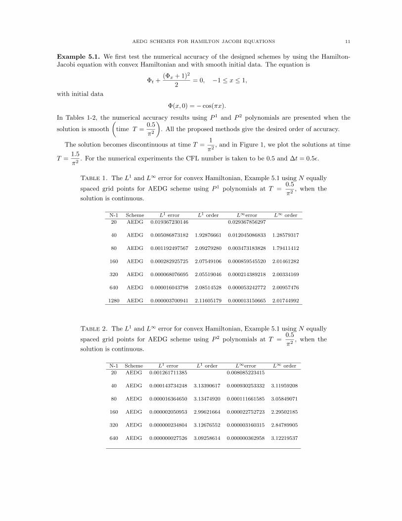
The solution becomes discontinuous at time T =1
π2, and in Figure 1, we plot the solutions at time
T =1.5
π2. For the numerical experiments the CFL number is taken to be 0.5 and ∆t = 0.5ε.
Table 1. The L1 and L∞ error for convex Hamiltonian, Example 5.1 using N equally
spaced grid points for AEDG scheme using P 1 polynomials at T =0.5
π2, when the
solution is continuous.
N-1 Scheme L1 error L1 order L∞error L∞ order
20 AEDG 0.019367230146 0.029367856297
40 AEDG 0.005086873182 1.92876661 0.012045086833 1.28579317
80 AEDG 0.001192497567 2.09279280 0.003473183828 1.79411412
160 AEDG 0.000282925725 2.07549106 0.000859545520 2.01461282
320 AEDG 0.000068076695 2.05519046 0.000214389218 2.00334169
640 AEDG 0.000016043798 2.08514528 0.000053242772 2.00957476
1280 AEDG 0.000003700941 2.11605179 0.000013150665 2.01744992
Table 2. The L1 and L∞ error for convex Hamiltonian, Example 5.1 using N equally
spaced grid points for AEDG scheme using P 2 polynomials at T =0.5
π2, when the
solution is continuous.
N-1 Scheme L1 error L1 order L∞error L∞ order
20 AEDG 0.001261711385 0.008085223415
40 AEDG 0.000143734248 3.13390617 0.000930253332 3.11959208
80 AEDG 0.000016364650 3.13474920 0.000111661585 3.05849071
160 AEDG 0.000002050953 2.99621664 0.000022752723 2.29502185
320 AEDG 0.000000234804 3.12676552 0.000003160315 2.84789905
640 AEDG 0.000000027526 3.09258614 0.000000362958 3.12219537
12 HAILIANG LIU AND MICHAEL POLLACK
−1 −0.5 0 0.5 1−1.5
−1
−0.5
0
0.5
1
ref
AE
(a) AEDG scheme with P 1 polynomials.
−1 −0.5 0 0.5 1−1.5
−1
−0.5
0
0.5
1
ref
AE
(b) AEDG scheme with P 2 polynomials
Figure 1. Comparison of plots for H-J equation with convex Hamiltonian, Example5.1, at discontinuity on [−1, 1], T = 1.5/π2, N = 81, using P 1 and P 2 polynomials.
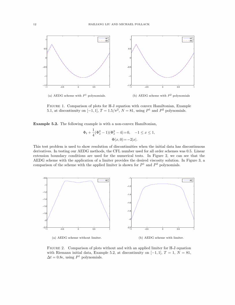
Example 5.2. The following example is with a non-convex Hamiltonian,
Φt +1
4(Φ2
x − 1)(Φ2x − 4)=0, −1 ≤ x ≤ 1,
Φ(x, 0)=−2|x|.
This test problem is used to show resolution of discontinuities when the initial data has discontinuousderivatives. In testing our AEDG methods, the CFL number used for all order schemes was 0.5. Linearextension boundary conditions are used for the numerical tests. In Figure 2, we can see that theAEDG scheme with the application of a limiter provides the desired viscosity solution. In Figure 3, acomparison of the scheme with the applied limiter is shown for P 1 and P 2 polynomials.
−1 −0.5 0 0.5 1−2.2
−2
−1.8
−1.6
−1.4
−1.2
−1
−0.8
AE
(a) AEDG scheme without limiter.
−1 −0.5 0 0.5 1−2.2
−2
−1.8
−1.6
−1.4
−1.2
−1
AE
(b) AEDG scheme with limiter.
Figure 2. Comparison of plots without and with an applied limiter for H-J equationwith Riemann initial data, Example 5.2, at discontinuity on [−1, 1], T = 1, N = 81,∆t = 0.8ε, using P 1 polynomials.
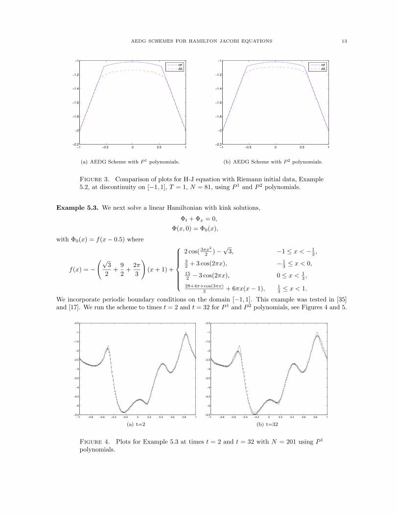
AEDG SCHEMES FOR HAMILTON JACOBI EQUATIONS 13
−1 −0.5 0 0.5 1−2.2
−2
−1.8
−1.6
−1.4
−1.2
−1
ref
AE
(a) AEDG Scheme with P 1 polynomials.
−1 −0.5 0 0.5 1−2.2
−2
−1.8
−1.6
−1.4
−1.2
−1
ref
AE
(b) AEDG Scheme with P 2 polynomials.
Figure 3. Comparison of plots for H-J equation with Riemann initial data, Example5.2, at discontinuity on [−1, 1], T = 1, N = 81, using P 1 and P 2 polynomials.
Example 5.3. We next solve a linear Hamiltonian with kink solutions,
Φt + Φx = 0,
Φ(x, 0) = Φ0(x),
with Φ0(x) = f(x− 0.5) where
f(x) = −
(√3
2+
9
2+
2π
3
)(x+ 1) +
2 cos( 3πx2
2 )−√
3, −1 ≤ x < − 13 ,
32 + 3 cos(2πx), − 1
3 ≤ x < 0,
152 − 3 cos(2πx), 0 ≤ x < 1
3 ,
28+4π+cos(3πx)3 + 6πx(x− 1), 1
3 ≤ x < 1.
We incorporate periodic boundary conditions on the domain [−1, 1]. This example was tested in [35]and [17]. We run the scheme to times t = 2 and t = 32 for P 1 and P 2 polynomials, see Figures 4 and 5.
−1 −0.8 −0.6 −0.4 −0.2 0 0.2 0.4 0.6 0.8 1−5.5
−5
−4.5
−4
−3.5
−3
−2.5
−2
−1.5
−1
−0.5
(a) t=2
−1 −0.8 −0.6 −0.4 −0.2 0 0.2 0.4 0.6 0.8 1−5.5
−5
−4.5
−4
−3.5
−3
−2.5
−2
−1.5
−1
−0.5
(b) t=32
Figure 4. Plots for Example 5.3 at times t = 2 and t = 32 with N = 201 using P 1
polynomials.
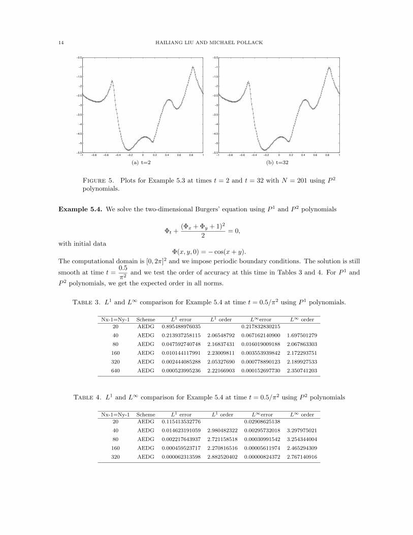
14 HAILIANG LIU AND MICHAEL POLLACK
−1 −0.8 −0.6 −0.4 −0.2 0 0.2 0.4 0.6 0.8 1−5.5
−5
−4.5
−4
−3.5
−3
−2.5
−2
−1.5
−1
−0.5
(a) t=2
−1 −0.8 −0.6 −0.4 −0.2 0 0.2 0.4 0.6 0.8 1−5.5
−5
−4.5
−4
−3.5
−3
−2.5
−2
−1.5
−1
−0.5
(b) t=32
Figure 5. Plots for Example 5.3 at times t = 2 and t = 32 with N = 201 using P 2
polynomials.
Example 5.4. We solve the two-dimensional Burgers’ equation using P 1 and P 2 polynomials
Φt +(Φx + Φy + 1)2
2= 0,
with initial dataΦ(x, y, 0) = − cos(x+ y).
The computational domain is [0, 2π]2 and we impose periodic boundary conditions. The solution is still
smooth at time t =0.5
π2and we test the order of accuracy at this time in Tables 3 and 4. For P 1 and
P 2 polynomials, we get the expected order in all norms.
Table 3. L1 and L∞ comparison for Example 5.4 at time t = 0.5/π2 using P 1 polynomials.
Nx-1=Ny-1 Scheme L1 error L1 order L∞error L∞ order
20 AEDG 0.895488976035 0.217832830215
40 AEDG 0.213937258115 2.06548792 0.067162140900 1.697501279
80 AEDG 0.047592740748 2.16837431 0.016019009188 2.067863303
160 AEDG 0.010144117991 2.23009811 0.003553939842 2.172293751
320 AEDG 0.002444085288 2.05327690 0.000778890123 2.189927533
640 AEDG 0.000523995236 2.22166903 0.000152697730 2.350741203
Table 4. L1 and L∞ comparison for Example 5.4 at time t = 0.5/π2 using P 2 polynomials
Nx-1=Ny-1 Scheme L1 error L1 order L∞error L∞ order
20 AEDG 0.115413532776 0.02908625138
40 AEDG 0.014623191059 2.980482322 0.00295732018 3.297975021
80 AEDG 0.002217643937 2.721158518 0.00030991542 3.254344004
160 AEDG 0.000459523717 2.270816516 0.00005611974 2.465294309
320 AEDG 0.000062313598 2.882520402 0.00000824372 2.767140916
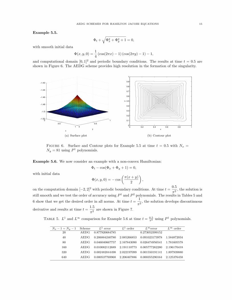
AEDG SCHEMES FOR HAMILTON JACOBI EQUATIONS 15
Example 5.5.
Φt +√
Φ2x + Φ2
y + 1 = 0,
with smooth initial data
Φ(x, y, 0) =1
4(cos(2πx)− 1) (cos(2πy)− 1)− 1,
and computational domain [0, 1]2 and periodic boundary conditions. The results at time t = 0.5 areshown in Figure 6. The AEDG scheme provides high resolution in the formation of the singularity.
0
0.5
1 0
0.5
1−1.52
−1.5
−1.48
−1.46
−1.44
−1.42
yx
(a) Surface plot
x
y
0 0.2 0.4 0.6 0.8 10
0.1
0.2
0.3
0.4
0.5
0.6
0.7
0.8
0.9
1
(b) Contour plot
Figure 6. Surface and Contour plots for Example 5.5 at time t = 0.5 with Nx =Ny = 81 using P 1 polynomials.
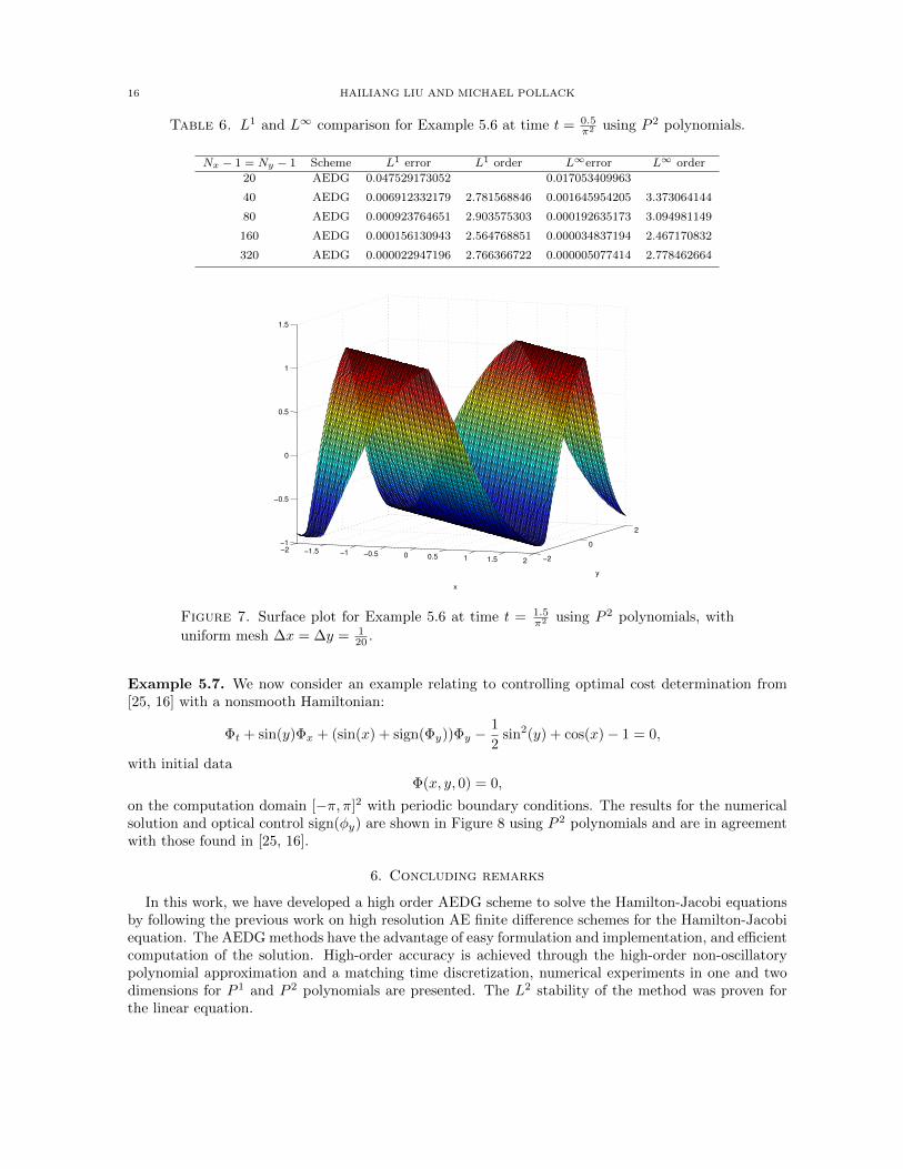
Example 5.6. We now consider an example with a non-convex Hamiltonian:
Φt − cos(Φx + Φy + 1) = 0,
with initial data
Φ(x, y, 0) = − cos
(π(x+ y)
2
),
on the computation domain [−2, 2]2 with periodic boundary conditions. At time t =0.5
π2, the solution is
still smooth and we test the order of accuracy using P 1 and P 2 polynomials. The results in Tables 5 and
6 show that we get the desired order in all norms. At time t =1
π2, the solution develops discontinuous
derivative and results at time t =1.5
π2are shown in Figure 7.
Table 5. L1 and L∞ comparison for Example 5.6 at time t = 0.5π2 using P 1 polynomials.
Nx − 1 = Ny − 1 Scheme L1 error L1 order L∞error L∞ order
20 AEDG 0.877920684785 0.273052399152
40 AEDG 0.206884240780 2.085266853 0.091023173978 1.584872034
80 AEDG 0.046040667757 2.167843090 0.026474956541 1.781605578
160 AEDG 0.010082112689 2.191110773 0.005777262280 2.196170418
320 AEDG 0.002482044498 2.022197099 0.001550191141 1.897939880
640 AEDG 0.000537769968 2.206467886 0.000355290164 2.125376458
16 HAILIANG LIU AND MICHAEL POLLACK
Table 6. L1 and L∞ comparison for Example 5.6 at time t = 0.5π2 using P 2 polynomials.
Nx − 1 = Ny − 1 Scheme L1 error L1 order L∞error L∞ order
20 AEDG 0.047529173052 0.017053409963
40 AEDG 0.006912332179 2.781568846 0.001645954205 3.373064144
80 AEDG 0.000923764651 2.903575303 0.000192635173 3.094981149
160 AEDG 0.000156130943 2.564768851 0.000034837194 2.467170832
320 AEDG 0.000022947196 2.766366722 0.000005077414 2.778462664
−2 −1.5 −1 −0.5 0 0.5 1 1.5 2 −2
0
2
−1
−0.5
0
0.5
1
1.5
y
x
Figure 7. Surface plot for Example 5.6 at time t = 1.5π2 using P 2 polynomials, with
uniform mesh ∆x = ∆y = 120 .
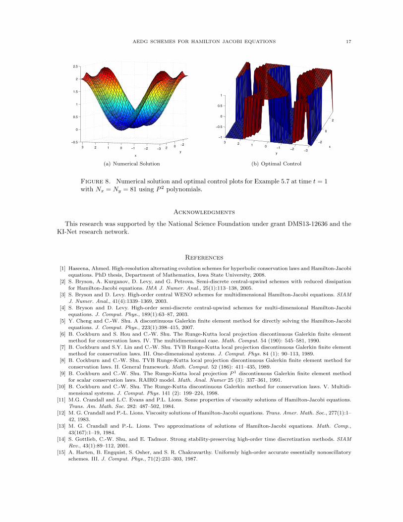
Example 5.7. We now consider an example relating to controlling optimal cost determination from[25, 16] with a nonsmooth Hamiltonian:
Φt + sin(y)Φx + (sin(x) + sign(Φy))Φy −1
2sin2(y) + cos(x)− 1 = 0,
with initial data
Φ(x, y, 0) = 0,
on the computation domain [−π, π]2 with periodic boundary conditions. The results for the numericalsolution and optical control sign(φy) are shown in Figure 8 using P 2 polynomials and are in agreementwith those found in [25, 16].
6. Concluding remarks
In this work, we have developed a high order AEDG scheme to solve the Hamilton-Jacobi equationsby following the previous work on high resolution AE finite difference schemes for the Hamilton-Jacobiequation. The AEDG methods have the advantage of easy formulation and implementation, and efficientcomputation of the solution. High-order accuracy is achieved through the high-order non-oscillatorypolynomial approximation and a matching time discretization, numerical experiments in one and twodimensions for P 1 and P 2 polynomials are presented. The L2 stability of the method was proven forthe linear equation.
AEDG SCHEMES FOR HAMILTON JACOBI EQUATIONS 17
−3−2−10123−2
02
−0.5
0
0.5
1
1.5
2
2.5
y
x
(a) Numerical Solution
−2
0
2
−3−2−10123
−1
−0.5
0
0.5
1
x
y
(b) Optimal Control
Figure 8. Numerical solution and optimal control plots for Example 5.7 at time t = 1with Nx = Ny = 81 using P 2 polynomials.
Acknowledgments
This research was supported by the National Science Foundation under grant DMS13-12636 and theKI-Net research network.
References
[1] Haseena, Ahmed. High-resolution alternating evolution schemes for hyperbolic conservation laws and Hamilton-Jacobi
equations. PhD thesis, Department of Mathematics, Iowa State University, 2008.[2] S. Bryson, A. Kurganov, D. Levy, and G. Petrova. Semi-discrete central-upwind schemes with reduced dissipation
for Hamilton-Jacobi equations. IMA J. Numer. Anal., 25(1):113–138, 2005.
[3] S. Bryson and D. Levy. High-order central WENO schemes for multidimensional Hamilton-Jacobi equations. SIAMJ. Numer. Anal., 41(4):1339–1369, 2003.
[4] S. Bryson and D. Levy. High-order semi-discrete central-upwind schemes for multi-dimensional Hamilton-Jacobiequations. J. Comput. Phys., 189(1):63–87, 2003.
[5] Y. Cheng and C.-W. Shu. A discontinuous Galerkin finite element method for directly solving the Hamilton-Jacobi
equations. J. Comput. Phys., 223(1):398–415, 2007.[6] B. Cockburn and S. Hou and C.-W. Shu. The Runge-Kutta local projection discontinuous Galerkin finite element
method for conservation laws. IV. The multidimensional case. Math. Comput. 54 (190): 545–581, 1990.
[7] B. Cockburn and S.Y. Lin and C.-W. Shu. TVB Runge-Kutta local projection discontinuous Galerkin finite elementmethod for conservation laws. III. One-dimensional systems. J. Comput. Phys. 84 (1): 90–113, 1989.
[8] B. Cockburn and C.-W. Shu. TVB Runge-Kutta local projection discontinuous Galerkin finite element method forconservation laws. II. General framework. Math. Comput. 52 (186): 411–435, 1989.
[9] B. Cockburn and C.-W. Shu. The Runge-Kutta local projection P 1 discontinuous Galerkin finite element method
for scalar conservation laws. RAIRO model. Math. Anal. Numer 25 (3): 337–361, 1991.
[10] B. Cockburn and C.-W. Shu. The Runge-Kutta discontinuous Galerkin method for conservation laws. V. Multidi-mensional systems. J. Comput. Phys. 141 (2): 199–224, 1998.
[11] M.G. Crandall and L.C. Evans and P.L. Lions. Some properties of viscosity solutions of Hamilton-Jacobi equations.Trans. Am. Math. Soc. 282: 487–502, 1984.
[12] M. G. Crandall and P.-L. Lions. Viscosity solutions of Hamilton-Jacobi equations. Trans. Amer. Math. Soc., 277(1):1–
42, 1983.[13] M. G. Crandall and P.-L. Lions. Two approximations of solutions of Hamilton-Jacobi equations. Math. Comp.,
43(167):1–19, 1984.
[14] S. Gottlieb, C.-W. Shu, and E. Tadmor. Strong stability-preserving high-order time discretization methods. SIAMRev., 43(1):89–112, 2001.
[15] A. Harten, B. Engquist, S. Osher, and S. R. Chakravarthy. Uniformly high-order accurate essentially nonoscillatory
schemes. III. J. Comput. Phys., 71(2):231–303, 1987.
18 HAILIANG LIU AND MICHAEL POLLACK
[16] C. Hu and C.-W. Shu. A discontinuous Galerkin finite element method for Hamilton-Jacobi equations. SIAM J. Sci.Comput., 21(2):666–690, 1999.
[17] G.-S. Jiang and D. Peng. Weighted ENO schemes for Hamilton-Jacobi equations. SIAM J. Sci. Comput., 21(6):2126–
2143, 2000.[18] L. Krivodonova, J. Xin, J.F. Remacle, N. Chevaugeon, J.E. Flaherty. Shock detection and limiting with discontinuous
Galerkin methods for hyperolic conservation laws. Appl. Numer. Math., 48:323–338, 2004.
[19] A. Kurganov, S. Noelle, and G. Petrova. Semidiscrete central-upwind schemes for hyperbolic conservation laws andHamilton-Jacobi equations. SIAM J. Sci. Comput., 23(3):707–740, 2001.
[20] A. Kurganov and E. Tadmor. New high-resolution semi-discrete central schemes for Hamilton-Jacobi equations. J.Comput. Phys., 160(2):720–742, 2000.
[21] D. Levy, S. Nayak, C.-W. Shu, and Y.-T. Zhang. Central WENO schemes for Hamilton-Jacobi equations on triangular
meshes. SIAM J. Sci. Comput., 28(6):2229–2247, 2006.[22] C.-T. Lin and E. Tadmor. High-resolution nonoscillatory central schemes for Hamilton-Jacobi equations. SIAM J.
Sci. Comput., 21(6):2163–2186, 2000.
[23] C.-T. Lin and E. Tadmor. L1-Stability and error estimates for approximate Hamilton-Jacobi solutions. Numer. Math.,87: 701–735, 2001.
[24] H. Liu. An alternating evolution approximation to systems of hyperbolic conservation laws. J. Hyperbolic Differ.
Equ., 5(2): 1–27, 2008.[25] F. Y. Li and S. Yakovlev. A central discontinuous Galerkin method for Hamilton-Jacobi equations. J. Sci. Comput.
45(1-3), 404–428, 2010.
[26] Y. Liu. Central schemes on overlapping cells. J. Comput. Phys., 209(1):82–104, 2005.[27] S. Osher and J. A. Sethian. Fronts propagating with curvature-dependent speed: algorithms based on Hamilton-
Jacobi formulations. J. Comput. Phys., 79(1):12–49, 1988.
[28] S. Osher and C.-W. Shu. High-order essentially nonoscillatory schemes for Hamilton-Jacobi equations. SIAM J.Numer. Anal., 28(4):907–922, 1991.
[29] W. H. Reed and T. R. Hill. Triangular mesh methods for the neutron transport equation. Technical Report Tech.Report LA-UR-73-479, Los Alamos Scientific Laboratory, 1973.
[30] H. Saran and H. Liu. Formulation and analysis of alternating evolution schemes for conservation laws. SIAM J. Sci.
Comput., 33: 3210–3240, 2011.[31] H. Liu and M. Pollack and H. Saran Alternating evolution schemes for Hamilton–Jacobi equations. SIAM J. Sci.
Comput., 35(1): 122–149, 2013.
[32] C.-W. Shu. High order ENO and WENO schemes for computational fluid dynamics. In High-order methods forcomputational physics, volume 9 of Lect. Notes Comput. Sci. Eng., pages 439–582. Springer, Berlin, 1999.
[33] J. Qiu and C.W. Shu. Hermite WENO schemes for Hamilton-Jacobi equations. J. Comput. Phys. 204: 82–99, 2005.
[34] P. E. Souganidis. Approximation schemes for viscosity solutions of Hamilton-Jacobi equations. J. Differ. Equ. 59:143, 1985.
[35] J. Yan and S. Osher. A new discontinuous Galerkin method for Hamilton-Jacobi equations. J. Comput. Phys. 230(1):
232–244, 2011.[36] Y.-T. Zhang and C.-W. Shu. High order WENO schemes for Hamilton-Jacobi equations on triangular meshes. SIAM
J. Sci. Comput., 24:1005–1030, 2003.
Iowa State University, Mathematics Department, Ames, IA 50011E-mail address: [email protected]; [email protected]


