Embed Size (px)
Citation preview

Olt,.fILECW
In
TECHNICAL REPORT ARCCB-TR-88024
A POSTERIORI ERROR ESTIMATION
'OF ADAPTIVE FINITE DIFFERENCE
SCHEMES FOR HYPERBOLIC SYSTEMS 0
DAVID C. ARNEYDTIC RPKSSAELECTE RUPAK B1SWASJUL 2 5 188 JOSEPH E. FLAHERTYS0
JUNE 19 8 8
US ARMY ARMAMENT RESEARCH,4 DEVELOPMENT AND ENGINEERING CENTER
CLOSE COMBAT ARMAMENTS CENTERBENiT LABORATORIES
WATERVLIET, N.Y. 12189-4050
APPROVED FOR PUBLIC RELEASE; DISTRIBUTION UNLIMITED
iSO H,, L - "''A
9,:e.

SECURITY CLASSIFICATION OF THIS PAGE (WhIen Date Entered) A M 8 76 &rREPORT DOCUMENTATION PAGE READ INSTRUCTIONS
BEFORE COMPLETING FORM1. REPORT NUMBER 2. GOVT ACCESSION NO. 3. RECIPIENT*S CATALOG NUMBER
ARCCB-TR-880244L TITL.E (anid $986tlo) S. TYPE OF REPORT & PERIOD COVERED
A POSTERIORI ERROR ESTIMATION OF ADAPTIVE FINITE FinalDIFFERENCE SCHEMES FOR HYPERBOLIC SYSTEMS . PERORMING OR. REPORT NUMBER
7. AUTHOR(e) S. CONTRACT OR GRANT NUMBER(o)
David C. Arney, Rupak Biswas, andJoseph E. Flaherty (See Reverse)
9. PERFORMING ORGANIZATION NAME AND ADDRESS 10. PROGRAM ELEMENT. PROJECT. TASK
AREA & WORK UNIT NUMBERS
US Army ARDEC AMCMS No. 6126.23.lBLO.0Benet Laboratories, SMCAR-CCB-TL PRON No. 1A72ZJ5MNMSCWatervliet, NY 12189-4050
I1. CONTROLLING OFFICE NAME AND ADDRESS 12. REPRT DATE
US Army ARDEC June 1988Close Combat Armaments Center 13. NUMBER OF PAGESPicatinny Arsenal, NJ 07806-5000 29
14. MONITORING AGENCY NAME A AOORESSe('! dItto t from Comtrolling office) 1|. SECURITY CLASS. (of this report)
UNCLASSIFIED
150. OECLASSIFICATION/OOWNGRAOINGSCHEDULE
1. DISTRIBUTION STATEMENT (of this Raeort)
Approved for public release; distribution unlimited.
17. DISTRIUTION STATEMENT (*I the abshract entered In Block 20, If different from Report)1 '1
IS. SUPPLEMENTARY NOTES
Presented at the Fifth Army Conference on Applied Mathematics and Computing,U.S. Military Academy, West Point, New York, 15-18 June 1987.Published in Proceedings of the Conference.
19. KEY WORDS jP tlnue on revere Oide It necesary and Identify by block number)
Hyperbolic Systems,Adaptive MethodsA Posteriori Error EstimationFinite Difference Methods .
MG AISTN ACT (fCrtilnsm anroe sa if necowea and Identify by block mmbw)
We describe several techniques that are based on Richardson's extrapolationfor estimating discretization errors of finite difference solutions of one-and two-dimensional hyperbolic systems. These a posteriori error estimatesare intended for use with adaptive mesh moving and local refinement procedures.Mesh moving algorithms produce nonuniform grids which necessitate specialtreatment of solution and error estimation techniques. The ...u.r 4 adjust-ments are discussed ,sing a two-step MacCormack method as a model finite
- (CONT'D ON REVERSE), ~ D pro n 143 COMO" or I Nov 6s Is O1MLtETE %
147 73 UNCLASSIFIED
SECUIT~Y CL.ASSIFICATIOWr OF THIS PAGE (When Does Entered)

SECURITY CLASSIFICATION OP THIS PAGE(IIFan Data Mnteed)
7. AUTHORS (CONT'D)
David C. ArneyDepartment of MathematicsUnited States Military AcademyWest Point, NY 10996-1786
Rupak BiswasDepartment of Computer ScienceRensselaer Polytechnic InstituteTroy, NY 12180-3590
Joseph E. FlahertyDepartment of Computer ScienceRensselaer Polytechnic InstituteTroy, NY Izi80-3590
and
US Army ARDECClose Combat Armaments CenterBenet LaboratoriesWatervliet, NY 12189-4050
20. ABSTRACT (CONT'D)
difference scheme. We also discuss automatic time step selection proceduresand the effects of artificial viscosity. Extrapolation schemes that produceseparate estimates of the temporal and spatial discretization errors arepresented and we show how these may be used to control local mesh refinementprocedures. Several examples illustrating these procedures are presented.
- 0740Li r
III
'-'-'I1 I' p
UNCLASSIFIED
SECUNITY CLASSIFICATION OF THIS PAGE(WP,.n Data Entered)

PIK,
TABLE OF CONTENTSPage
INTRODUCTION 1
SOLUTION SCHEME 2
MacCormack Scheme 2
Variable Time Step 5
Artificial Viscosity 6
ERROR ESTIMATION 7
Richardson's Extrapolation Error Estimation 8
Error Estimation for a Moving Nonuniform Mesh 10
COMPUTATIONAL EXAMPLES 12
Example 1 13
Example 2 17
Example 3 20
Example 4 21
CONCLUSION 23
REFERENCES 25
TABLES -a
I. EXACT AND ESTIMATED ERRORS FOR DIFFERENT MESH SIZES FOR EXAMPLE 2 17
II. EXACT AND ESTIMATED ERRORS FOR DIFFERENT MESH STRATEGIES FOR 21EXAMPLE 3 S
a,'III. EXACT AND ESTIMATED ERRORS FOR DIFFERENT MESH STRATEGIES FOR 23
EXAMPLE 4
LIST OF ILLUSTRATIONS 0
1. Spatial structure of the moving coarse mesh with embedded fine mesh 12used for the error estimation.
2. Initial mesh for Example 1. 14

Paqe
3. Mesh of Example 1 at t = 1.6. 15
4. Mesh of Example 1 at t = 3.2. 15
S. Contour plots of the solutions of Example 1 on a moving mesh 16without artificial viscosity and with artificial viscosity att = 3.2.
6. Surface plots of the solutions of Example I on a moving mesh 16without artificial viscosity and with artificial viscosity att = 3.2.
7. Adaptive mesh of Example 2. 18
8. Solutions at base time steps for the adaptive local refinement 19procedure of Example 2.
"V
..
i i ..
o°5
5%.

INTRODUCTION
With the use of adaptive methods to solve time-dependent partial differen-
tial equations, there exists a requirement to compute solutions on moving nonu-
niform grids. There is also a requirement to estimate the local discretization
error as feedback to modify or refine the mesh. In this report, we discuss the
MacCormack finite difference scheme and a Richardson extrapolation-based error
estimation procedure that was used in the adaptive algorithm of Arney (ref 1)
and Arney and Flaherty (refs 2,3) to solve time-dependent hyperbolic systems in "
one- and two-space dimensions. Examples of other adaptive methods with these
requirements are Rai and Anderson (ref 4), Adjerid and Flaherty (ref 5), Bell
and Shubin (ref 6), and Davis and Flaherty (ref 7).
Finite difference methods use a mapping to transform the time and space
variables from a moving nonuniform mesh to a stationary uniform mesh. The
method used to compute the metrics of this transformation must be carefully cho-
sen in order to preserve the stability, conservation, and accuracy of the scheme
(cf. Thomas and Lombard (refs 8,9) and Hindman (refs 10,11)).
The MacCormack finite difference scheme has had wide use in solving
Eulerian conservation laws for fluid dynamics. The recent use of artificial
viscosity to make this scheme total variation diminishing (TVD) makes it more
attractive as a general solver for problems with discontinuities (cf. Davis (ref N
(12) and Roe (13)). In the following section, we discuss the MacCormack scheme,
our implementation of the differencing of the metric terms, adaptive selection
of the time step, and the TVD artificial viscosity of Davis (ref 12). The
Richardson's extrapolation-based error estimation method produces a pointwise
approximation of the local discretization error which can be used to construct
References are listed at the end of this report.

several global measures of the discretization Grror. Next, we discuss our error %
estimate and its implementation on a moving mesh. Then we present computational
results of solutions of hyperbolic problems. Computations were performed in
one- and two-dimensions on stationary uniform and moving nonuniform grids.
Lastly, we discuss the utility of our methods, the computational results, and
future work.
SOLUTION SCHEME
Consider the hyperbolic vector systems of conservation laws in two-space
dimensions
ut + fx(x,y,u,t) + gy(x,y,u,t) = 0 , (x,y) e D, t > 0 (1)
u(x,y,O) = Uo(x,y), (x,y) e D U 8D, (2)
with appropriate well-posed conditions on the boundary 3D of a rectangular
domain D.
We chose to implement the MacCormack finite difference scheme for hyper-
bolic problems because of its general applicability. The MacCormack scheme,
like most higher-order methods, will suffer a reduction in order on a moving
nonuniform grid. Despite this fact, proper mesh moving and node placement by an "
effective adaptive procedure provide enough efficiency and accuracy to compen-
sate for this order reduction.
MacCormack Scheme
In order to discretize Eq. (1), we introduce a transformation
= (x,y,t), n = n(x,y,t), T = t, (3)
from the physical (x,y,t) domain to a computational (1,n,T) domain where a uni-
form rectangular grid will be used. Under this transformation, Eq. (1) becomes
UT + utt + unnt + fcx + fqnx + gty + gry = 0 (4)
2
-.. ,<

0
The transformation metrics (Cx,Cytt,nx,ny,nt) are related to the metrics
(XCXnXT~yynyT) by the identities
X = . ,nt: J (YX2_STYD) _ _Yt
=-' = J, t = ..... , x =-j- ,
=xx (yXT-XY T )ny - = J = YnX - xnY(5)
Using Eq. (5) in Eq. (4) gives
--- -(yx -xY ) y -- - - + + X 0 (6)UT + ;t ( ) -
This equation can be rewritten in another form in the original transformation,1#
metrics by further substitutions of Eq. (5) into Eq. (2) as
UT - Ut(XTtx+YTy) - Un(XTnx+yTny) + fttX + fnnx + gty + gqny = 0 (7)
Some authors (cf. Hyman (ref 14) and Thompson (ref 15) prefer to write this V.
equation in still another form as
uT + -gt + unnt + f{tx + gy + gnny =0 (8)S
A uniform space-time grid having mesh spacing At x An x AT is introduced
onto the computational domain. The finite difference solution at (M4 , mAn, ?
-n .nAT) is referred to as ujm. A similar notation is used for the fluxes f and g
and the metrics in Eq. (5). The two-step MacCormack scheme (ref 16) uses first-
order forward temporal and spatial difference approximations in the predictor
step, and first-order backward differences in the corrector step. The predicted
-n+1solution Im satisfies ft.tf
-n+1 -n AT -n -n n -n -n n22'm = Im - I [(u+1,m-uIm)(Rt)Im + (fI+I'm-fjm)(x)i'm
+ n -n n AT -n -n n •+ (gi+lm-gim)(Ry)I,m] - Z5 f(uI'm+1-UI'm)(qt)I'm
-n -n n -n -n n
+ (fi,m+l-fIm)(nx)im + (gim+1-gIm)(ny),m] (9).
3

p
nThe metrics (x)1,m, etc. are computed by forward differences. The corrected
-n+1solution uI,m satisfies
-n+1 1 -n -n+l AT -n+1 -n+1 n+1 -n+l -n+1 n+1 -
U,m = {U(,m + _Im - 1 ((Y,m-2-1,m)(Rt)im + (fm-f-1,m)(x)fm
+ n+1 -n+1 n+l AT -n+1 -n+1 n+1+ ( ,m -lm)(y) m]- j [(3 ,m-i,m-1)(flt)I,m
n+l -n+1 n+1 -n+1 -n+1 n+1 ..+ ( I,m-f,m-1)(x)i,m + (gi,m-i,m-1)(y)i,m]} (10)
-n+1with metrics computed by backward differences. The notation fm denotes-n+1
f(jj,m), etc. The use of first forward and backward difference approximations
for the metrics implies that the transformation from the computational to the
physical domain is piecewise trilinear in space and time for the predictor and
corrector steps. Such low order difference approximations are responsible for
reducing the orders of the MacCormack scheme. A smoother transformation and the
use of higher-order difference approximations of the metrics could be used to
maintain secord order accuracy.
It was shown by Hindman (refs 10,11) that this differencing of Eq. (6) pro- N
duces consistent approximations. Therefore, a uniform flow solution is main-
tained. Other conservative forms for the transformed equations were
investigated by Hindman (ref 10) and found to be less efficient or needing spe-
cial differencing of the metrics for computing consistent approximations. p
Equation (4) is conservative on a moving mesh. We show this for a one-
dimensional scalar conservation law by investigating the Rankine-Hugoniot jump
conditions across a shock discontinuity. Consider a conservation law in the
form
a (f u dx) + f(u)l = 0 (11)t4
4-
• -.- ......- -.-- .-' -. -. - - " -- .'-."-."-.V ."'-' --'-."-.--. - .-.-- .---' .. :.-.- -.. .. .. ." -".." .'. ..'.. ..',-' " :):

.. .. , . . ..I J .
,J.
The jump conditions for a discontinuity at x = s(t) satisfy
Cu l (12)(u]
where (q] indicates the jump in q, and s= s denotes the shock velocity (ref
17).
A conservation law on a moving mesh produced by a transformation of
Vpvariables to a uniform stationary mesh satisfies V
+ rt ) f uxtdt + f(u) = 0 (13)
T) -0 0
Assuming the existence of a shock discontinuity, { = r(T) gives
xu + f )Td + f (uxt)Td + f(u)J = 0 (14)W r -00
Using the chain rule provides an integrable form
rxt[u* + fr (ux--f)df + J (uxr-f) dC + f(u)) = 0 (15) 8
Integration of this equation gives jump conditions in the computational domain
asV
rx [u] - +f] + xT.u] = 0 (16)
Since s(t) and r(T) are related by
s = r x + xT (17)
the appropriate jump condition in Eq. (12) is recovered.
Variable Time Step
The explicit MacGormack scheme has a stability restriction that limits the
time step allowed for a given spatial mesh. For efficient computation, the time
step should be adaptively set close to the maximum allowed by the Courant, P
Friedrichs, Lewy theorem (ref 18) ,
N

AT (18)2Y'2 max(w,,w)
The computational mesh has been selected to have spacing AC = An = 1 and the
constant 0.8 provides a 20 percent margin of safety. The quantities t and w are
the spectral radii of one-dimensional conservation laws on moving meshes, i.e.,
= max(Xi-XT)tX + (Pi-YT)Cy] (19a)
w = max[(Xi-XT)nX + (Pi-YT)ny] (19b)
where Xi and pi are eigenvalues of fu(u) and gu(u). These eigenvalues and the
metrics in Eqs. (19a) and (19b) are evaluated at the beginning of each time
step.
Artificial Viscosity
The MacCormack scheme, being a second order accurate centered scheme, pro-
duces spurious oscillations near discontinuities. In order to eliminate or
reduce these oscillations, artificial viscosity or dissipation is added to the
solution to diffuse the discontinuity. The viscosity is often problem-
dependent, and considerable "fine tuning" is usually needed to balance the
effects of the spurious oscillations and diffusion (ref 19).
We use an artificial viscosity model due to Davis (ref 12) which is not
problem-dependent and only requires knowledge of * and w. This artificial
viscosity model is designed to convert the MacCormack scheme into a total
variation diminishing (TVD) scheme in one-dimension. A scheme is TVD if the
total variation of the solution to an initial value problem is nonincreasing in 1%
time. Recent research efforts have resulted in the development of other second I
order accurate TVD schemes (cf. Osher and Chakravarthy (ref 20) and Warming and
Beam (ref 21)). .
.0
6

The artificial viscosity of Davis (ref 12) is based on a flux limiter that J:
dosnot depend on explicitly determining the upwind direction and, with a
recent modification by Roe (ref 13), does not affect the region of stability of "
the MacCormack scheme. Because the MacCormack scheme also does not determine
the upwing direction, the combined use of the MacCormack scheme and Davis' arti-
ficial viscosity is computationally simpler to perform than many other TVD
schemes. The artificial viscosity terms are calculated from the solution data
at the beginning of the time step. For two-dimensional problems, separate
dissipative terms are calculated in the t and n directions, resepectively.
ERROR ESTIMATION
Accurate a posteriori error estimation is an integral part of an adaptive
software system. Error estimation can be the most expensive part of an adaptive
procedure and an important goal is to find accurate and inexpensive ways of
,.
estimating the discretization error (cf. Babuska, et al. (refs 22,23)). The a
error estimatin on expity detenntemany factors, including the type of
solver used in the algorithm, the type of error to be determined, and the norm
in which the error -stimate is to be measured. It is most desirable to have aprocedure that provides pointwise estimates of the error which can then be used
to find estimates in several local and global norms. .
Mesh nonuniformity affects the accuracy and convergence of numerical
schemes and error estimation. The effects of the mesh on the solution scheme
have been studied by Ciment (ref 24), Fritts (ref 25), Hoffman (ref 26), Osher.-
and Sanders (ref 27), Sanders (ref 28), and Mastin (ref 29). Error analysis
seems to be more natural and further developed for finite element schemes, espe-
cially for elliptic )d parabolic problems (cf. Adjerid and Faherty (refs 5,
30), Zienkiewicz et al. (refs 31,32), and Babuska and Rheinboldt (refs 33,34)),
N 3
% .
proedrean a ipotat galistofid ccrae ad nepesie ay o

where relatively inexpensive local calculations are used to provide accurate
global spatial error estimates. More study needs to be done to find less expen-
sive and more accurate error estimates for finite difference schemes for hyper-
bolic problems.
We calculate the local temporal and spatial portions of the discretization
error, using an algorithm based on Richardson's extrapolation. Flaherty and =5
Moore (refs 35,36) and Berger and Oliger (ref 37) also use Richardson's extrapo-
lation to estimate error on uniform meshes for their local mesh refinement
algorithms.
Richardson's Extrapolation Error Estimation
We develop the error estimation for the second order MacCormack scheme for
a linear scalar problem in two dimensions. Separate pointwise estimates at a
tgeneral spatial node i, at time t, for the local temporal error Ei(t) and local
s ,spatial error Ei(t) are obtained with two different extrapolation procedures.
Consider a uniform mesh with spacing Ax x Ay and time step At. Let the
exact solution at node i and time t be denoted as ui(t), the numerical solution
by the MacCormack scheme at the same point and time as Ui(t;Ax,Ay,At), and the
MacCormack finite difference operator as L(Ax,Ay,At), i.e.,
Ui(t+At;Ax,Ay,At) = L(Ax,Ay,At)Ui(t;Ax,Ay,At) (20)
Assume that the local error has a Taylor's series expansion of the form
ui(t) - Ui(t;Ax,Ay,At) = At[clAtz + c2Ax2 + c3AY2 + ... 1 (21)
where the constants ci, c2 , c3 .... are independent of the mesh spacing....
To estimate the spatial component of the error, we calculate a solution on
a mesh of double spatial size (2Ax x 2Ay) with the same time step (At). The
local error on this mesh satisfies
ui(t+At) - Ui(t+At;2Ax,2Ay,At) = At[cjAt2 + 4c2Ax2 + 4c3AY2 + ... ] (22)
8
8 5V.5
1 I

Subtracting Eq. (22) from Eq. (21) and neglecting higher order terms, we "
obtain an expression for the leading term in the spatial portion of the local
error for the MacCormack scheme on the Ax x Ay x At mesh assEi(t+At):= At(c 2 Ax
2 + C3AY 2 ]
3 iUi(t+At;2Ax,2Ay,At) - Ui(t+At;Ax,Ay,At)] (23)
Similarly, an estimate of the temporal portion of the local error,t
Ei(t+At), can be calculated by computing another solution on the Ax x Ay spatial
mesh using two time steps of At/2, subtracting this result from Eq. (21), and 0
retaining the leading order term as
tEi(t+At):= At(clAt2 ]
4 At= (Ui(t+4t;Ax,Ay,2(4-)) - Ui(t+&t;Ax,Ay,&t) ] (24)
The leading term of the local error at node i and time t+At ist s
Ei(t+At) = El(t+At) + Ei(t+At) (25)
There are several disadvantages to this technique that should be noted: (1)
the error cannot be calculated for nodes on or adjacent to the boundary; (2) the
solution must be smooth enough for the cl, c2 , and c3 to exist; (3) the error ®
.estimation costs approximately three times more to compute than the solution; A
and (4) the mesh must be uniform. Equation (25) may still be useful as a mesh
refinement or motion indicator even in situations where jumps in the solution
render it invalid as an estimate of the error.
Richardson's extrapolation can be done in a more classic manner provided
that we are willing to forego separate spatial and temporal error estimates.
Thus, the error at node i in a solution on a mesh having spacing Ax x At is
estimated by calculating a second solution on a mesh with spacing Ax/2 using two
time steps of At/2. According to Eq. (22), the local error on this mesh
.9

satisfies
ui(t+At) - Ui(t+At;Ax/2,2(&t/2)) = At(C1At2/4 + c2Ax
2/4 + ... ] (26)
Subtracting Eq. (26) from Eq. (22) and neglecting higher order terms, we
can obtain error estimates for either Ui(t+at;ax,at) or Ui(t+At;Ax/2,2(At/2)) 0
provided that node i is common to both meshes. Our adaptive method carries the
fine grid solution forward in time; thus, we estimate its error as
Ei(t+At) = h At(clht2+c2Ax2 )
-& x At
= fUj(t+at; 4- 2(4-)) - Ui(t+&t;Ax,At)] (27)3 2 2
Using this procedure, the error can now be calculated at nodes adjacent to
boundaries. Even though this error estimate costs four times more to compute
than the solution, we only incur this overhead in the first time step. No addi-
tional cost is incurred if portions of the mesh have to be refined because the
solution on the refined mesh has already been computed and stored while esti-
mating the error for the coarser parent mesh.
Error Estimation for a Moving Nonuniform Mesh
Nonuniformity of the mesh changes the discretization error of the
MacCormack scheme. For simplicity, we will determine this error and analyze its
effects on the Richardson extrapolation error estimation using a linear scalar
problem in one-space dimension
ut + bux = 0 (28)
The local error for the MacCormack method on a one-dimensional moving nonu-
niform mesh is
b n+1 nui(t+At) Ui(t+At;Ax,At) = At[- (Axr -Axi)uxx
Atb 2 (1 x(-)uxx) + ClAt2 + c 2Ax2] (29)
Axn N
10
101

n nwhere Ax1 and Axr are the mesh sizes on the left and right node i at time step
n+1 n+1n, respectively, and Ax = max(Axr ,AxJ ). On the moving nonuniform mesh, both
J.the temporal and spatial error components contain second order terms, whereas 1
the error on a uniform mesh is third order. The previous analysis can be used .
to show that the leading component of the temporal error is
t Axn+1Ei(t+At):= At[- AtbZ(1- ------ )uxx]
AxnIV
At 0- 2[Ui(t+At;Ax,2(4-)) - Ui(t+At;Ax,At)] (30)
Calculation of the spatial portion of the error is more difficult since the '
temporal portion of the error does not cancel upon subtraction of solutions
calculated on two spatially different meshes. We overcome this difficulty and
also greatly simplify the procedure in two dimensions by constraining the mesh
to maintain double size increments for special nodes of the moving coarse mesh.S
This constrained grid structure consists of a coarse mesh, shown with darker
lines in Figure 1, containing properly nested fine cells created by binary divi-
sion of the sides of the coarse cells, shown by lighter lines in Figure 1. The
vertices of the coarse cells are denoted as "independent moving nodes." Error
estimates are calculated for these nodes. The remaining nodes in the mesh of
Figure 1 are "dependent moving nodes" which must be moved to maintain the
constrained grid structure. A solution is computed for these "dependent moving
nodes," but no error estimate is obtained.
For the "independent moving nodes," the spatial error calculation can
proceed as for a uniform mesh; therefore, the local spatial error estimate is
s n+Ei(t+At) = At[- (Axr X)uxx]
Ui(t+At;Ax,At) - Ui(t+At;2Ax,At) (31)
11'4

AL
Figure 1. Spatial structure of the moving coarse mesh (bold lines) withembedded fine mesh (fine lines) used for the error estimation.
The above analysis extends directly to two dimensions; hence, we have a
Richardson extrapolation-based procedure of estimating error on a moving nonuni-
form grid. In practice, we test the need for local uniformity and, if found,
use formulas in Eqs. (23) through (25) to compute error estimates.
Error estimation for systems of equations involves the use of a vector norm
at node i and time (t). The examples in the following section use the maximum
norm, i.e.,
Ei(t) max I Eij(t)I (32)
1 4j 4 N
where N is the number of equations in the system and Eij(t) is the local error
estimate for the jth component of the solution vector at node i.
COMPUTATIONAL EXAMPLES
The solution and local error estimation procedures are applied to four
examples. In Example 1, we demonstrate the capability of the MacCormack scheme
with Davis' TVD artificial viscosity on a moving nonuniform mesh. In Example 2,
we investigate a one-dimensional problem using a modified form of the error
12
Lz,%S

estimate in Eqs. (27) and (28). Examples 3 and 4 illustrate the performance of
the error estimation procedure on a problem having a smooth solution and one
with a jump in the first derivative, respectively. We investigate the accuracy
and convergence of the local error estimator by determining an effectivity index N
IIEtlle = Tle-- (33a)
at a fixed time t for several different meshes and different adaptive strate-
gies. Here e and E are the exact and estimated errors, respectively. The LI
norm,
IIEII1 := If Edxdy (33b)
is obtained by assuming E to be a piecewise constant function.
Example 1
Consider the initial-boundary value problem -
ut - yux + xuy = 0, t > 0, -1.2 4 x 4 1.2, -1.2 4 y 4 1.2 (34)12 1
u(x,y,O) = (x - ) + 1.5y
1 - 16((x - ) + 1.5y2 ) , otherwiseL!and
u(1.2,y,t) = u(-1.2,y,t) = u(x,-1.2,t) = u(x,1.2,t) = 0 (36) '
-t 0 if C < 0 -%u(x,y,t) = -(37) .aL , if C) 0
where
2C = 1 - 16((xcost + ysint - ) + 1.5(ycost - xsint)2 ) (38) '
Equations (37) and (38) represent a moving elliptical cone rotating coun-
terclockwise around the origin with period 2n. This problem was proposed as a
test problem by Gottlieb and Orszag (ref 38) and was used as a test problem in a
s4esurvey by McRae et al. (ref 39).
13

We show the sequence of meshes that were generated at t 2 o, 1.6, and 3.2
using the adaptive mesh moving method of Arney and Flaherty (ref 2) in Figures
2, 3, and 4, respectively. Arney and Flaherty's mesh moving method (ref 2) uti-
lizes the error estimates (see Error Estimation section of this report) to con-
centrate the mesh in the high-error region beneath the cone and to follow it as
it rotates. It also increases the accuracy of the solution and reduces oscilla-
tions in the wake following the cone. However, small oscillations are still
present. Next, we solve this problem with the same moving mesh technique byS
using Davis' artificial viscosity (ref 12) with the MacCormack scheme. Surface
and contour plots of solutions with and without artificial viscosity are shown
in Figures 5 and 6. There is no artificial wake behind the cone when artificial
viscosity is used. However, the artificial viscosity slightly diffuses the
cone, widening its base and reducing its peak from 1.0 to 0.88.
Fi 2 In ii m f E le 1I FI IF!IIltI i'IIF __14I I iI! I :l I I
I I !!ItFJii
Figure 2. Initial mesh for Example 1.
5%'.
%I.
• • • -' ' ", . . ,- ., .,., - -.14, .. , . . '

Figure 3. Mesh of Example 1 at t =1.6. Nodes have moved with therotating cone.
Figure 4. Mesh of Example 1 at t =3.2. Nodes have moved with thecone for one-half rotation.
15
IwoP

.6 .I
10I20
Figure 5. Contour plots of the solutions of Example I on a moving meshwithout artificial viscosity (left) and with artificialviscosity (right) at t =3.2.
%.5.
Figure 6. Surface plots of the solutions of Example I on a moving meshwithout artificial viscosity (top) and with artificialviscosity (bottom) at t a 3.2.
16
, -'.
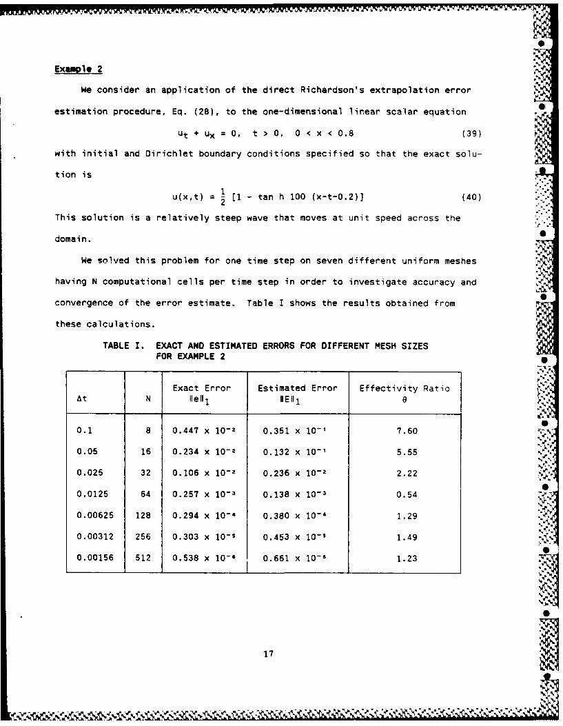
Example 2
We consider an application of the direct Richardson's extrapolation error
estimation procedure, Eq. (28), to the one-dimensional linear scalar equation S
Ut + ux = 0, t > 0, 0 < x < 0.8 (39)
with initial and Dirichlet boundary conditions specified so that the exact solu-
tion is
u(x,t) = [1 - tan h 100 (x-t-0.2)] (40)
This solution is a relatively steep wave that moves at unit speed across the
domain.
We solved this problem for one time step on seven different uniform meshes
having N computational cells per time step in order to investigate accuracy and
convergence of the error estimate. Table I shows the results obtained from
these calculations.
TABLE I. EXACT AND ESTIMATED ERRORS FOR DIFFERENT MESH SIZESFOR EXAMPLE 2
Exact Error Estimated Error Effectivity RatioAt N lell1 IEI11 e
0.1 8 0.447 x 10- 2 0.351 x 10⁻¹ 7.60 .,?
0.05 16 0.234 x 10² 0.132 x 10⁻¹ 5.55
0.025 32 0.106 x 10⁻² 0.236 x 10⁻² 2.22
0.0125 64 0.257 x 10⁻³ 0.138 x 10 -
3 0.54
0.00625 128 0.294 x 10⁻⁴ 0.380 x 10⁻⁴ 1.29
0.00312 256 0.303 x 10- s 0.453 x 10-s 1.49
0.00156 512 0.538 x 10⁻⁶ 0.661 x 10⁻⁶ 1.23
17

Vi Vf W
We also solved this problem using Arney and Flaherty's adaptive local
refinement procedure (ref 3) on a base mesh having Ax = At =0.1 with a local
error tolerance of 1/128. The mesh created by the local refinement algorithm-
is shown in Figure 7 and the solutions computed at each base time step are shown
in Figure 8.
0.,20 0.40 0.60 0.90 1.00
Figure 7. Adaptive mesh of Example 2.
18 *

"vC
. .4L4
&A IL&
4
424
Figure 8. Solutions at base time steps for the adaptive local rrefinement procedure of Example 2.
The adaptive composite mesh of Figure 7 shows a distinct pattern associated .,with using the MacCormack scheme with our local refinement strategy. Spacious '
oscillations of the solution on the base mesh cause several levels of refinement .which drastically reduce the base mesh spacing at the beginning of each base
time step. However, once these oscillations have been controlled, the need for""
refinement is reduced at the later stages of the adaptive procedure. Thissituation could be alleviated by including an artificial viscosity model withthe MacCormack scheme.
OW .
& 40
4 4
4 4 4 19

* -- - -. - i. , L.7 . w , , .w - -
Example 3
Consider the linear scalar hyperbolic differential equation
ut + 2Ux + 2 uy = 0, t > 0, 0.2 4 x 4 1.2, 0 > y 1 (41)
with initial conditions
u(x,y,O) = (1-tan h 3(x-0.+0.1)) (42) ,2
and with Dirichlet boundary conditions specified so that the exact solution of
this problem is
u(x,y,t) = (1-tan h 3(x-O.1 -1.St+0.1)(43)2
This solution is a smooth wave that moves at an angle of 45 degrees across
the domain. The problem was selected to show the convergence and accuracy of
Richardson's extrapolation error estimation procedure (Eqs. (28) and (29)). We
solve Eqs. (41) and (42) for one time step, At = 0.012, on eight different
meshes. The mesh strategy of each calculation is described as follows:
1. a stationary uniform (10 x 10) rectangular mesh
2. a stationary uniform (20 x 20) rectangular mesh
3. a stationary uniform (40 x 40) rectangular mesh
4. a stationary uniform (60 x 60) rectangular mesh
5. a stationary (40 x 40) mesh of nonuniform quadrilateral cells
6. a moving (20 x 20) mesh with uniform rectangles
7. a moving (20 x 20) mesh of nonuniform quadrilateral cells
8. a moving (40 x 40) mesh of nonuniform quadrilateral cells
Table II shows the results from these calculations by comparing the exact errors
and the effectivity indices for the eight strategies.
20
-. ' **j~j~* *~V*~~f~ V 'V~ *~%'-~.'% %V

,%.-k .. . . , ,*.. .;. ,,
Wr
,dp.
TABLE II. EXACT AND ESTIMATED ERRORS FOR DIFFERENT MESHSTRATEGIES FOR EXAMPLE 3
Mesh Strategy Exact Error Estimaced Error Effectivity Ratio(From Above) Ilell1 IIEII1 "
1 0.0111 0.0071 0.64
2 0.00370 0.00318 0.86
3 0.000942 0.000908 0.96
4 0.000367 0.000368 1.00
5 0.000399 0.000418 1.04
6 0.00136 0.00124 0.91ON
7 0.000411 0.000370 0.90
8 0.000167 0.000156 0.94
Strategies 1 through 4 show the convergence of the error estimates on uni-
form meshes as the number of nodes increases. These errors show a rate of con-
vergence of 0(AX2,Ay2 ) which is predicted in Eq. (21). Comparison cf the errors
of strategies 3 and 5 shows the error is cut in half by computing with a better IN
nonuniform stationary mesh. Further comparison of strategies 5 and 7 shows
another reduction of error by half when the mesh is properly moved. The nonuni-
formity of the mesh in strategies 5, 7, and 8 produces little change in the
effectivity of the error estimation. These nonuniform mesh comp'tations indi-
cate a convergence rate 0(Axl. 32,Ayl. 3 2 ).
Example 4
Consider the linear scalar hyperbolic differential equation .
ut + ux + 0.25uy = 0, t > 0, 0.2 < x 4 1.2, 0 < y < 1 (44)
21
,'00
):2I-/

with initial conditions
0 if y < -4x + 1.2 N
u(x,y,O) = 0.8 if y > -4x + 1.6 (45) N.,
-8x - 2y + 3.2 , otherwise,
and with Oirichlet boundary conditions
0 if y - 0.25t < -4(x-t) + 1.2
u(x,y,O) = - , y - 0.25t > -4(x-t) + 1.6 (46)
-8(x-t) 2(y-0.25t) + 3.2, otherwise.
The solution of this problem is an oblique ramplike wave front that moves
at an angle of 14 degrees across the domain. The solution has a jump in its
first partial derivatives at the top and bottom edges of the wave front. we
expect some difficulty in estimating the error near locations where the deriva-
tives jump. In the region of the front itself, the gradient of the solution is
constant and there is no error in the solution or in the error estimate.
We solved this problem for one time step, At = 0.015, for the following six
mesh strategies:1. a stationary uniform (12 x 12) rectangular mesh
2. a stationary uniform (24 x 24) rectangular mesh3. a stationary uniform (48 x 48) rectangular mesh
4. a stationary uniform (64 x 64) rectangular mesh
4. a stationary unifor2(64 x 64) reshngf ual
5. a stationary (24 x 24) mesh of nonuniform quadrilateral cells
6. a moving (24 x 24) mesh of nonuniform quadrilateral cells.
Table III shows the results of these strategies.
'2-
22

TABLE III. EXACT AND ESTIMATED ERRORS FOR DIFFERENT MESH STRATEGIES FOREXAMPLE 4. THE ERROR ESTIMATE IS ACCURATE, BUT THE SOLUTIONAPPEARS TO BE CONVERGING
Mesh Strategy Exact Error Estimated Error Effectivity RatioNell1 NEli1 e
1 0.0058 0.0016 0.28
2 0.00275 0.00110 0.40
3 0.000866 0.000479 0.55
4 0.000400 0.000222 0.56
5 0.00144 0.00078 0.54
6 0.000720 0.000349 0.49
The results are once again as expected. The error estimate of this problem
with a jump in the derivative is not as accurate as the smooth solution of
Example 3. However, the error estimate still shows signs of converging to the
exact error in L1 for the uniform meshes of strategies 1 through 4. Once again,
the better nodal placement of the initial mesh by the mesh generator of Arney
(ref 1) reduces the error by half from a uniform mesh. Also, moving the mesh by
the method of Arney and Flaherty (ref 2) reduces the error by half again.
CONCLUSION
We have shown that MacCormack's finite difference scheme and error estima-
tion based on Richardson's extrapolation can be used on moving grids with local
refinement. With proper computation of the transformation metrics and the use
of TVD artificial viscosity, the MacCormack scheme is stable and is able to
solve problems with sharp discontinuities.
23
%%%
The examples we have presented demonstrate the utility of these methods and
also point out their shortcomings. Of particular concern is the lack of any
error estimation near the boundaries, the poor error estimation near discon-
tinuities, and the need to constrain the mesh to obtain any accurate error esti-
mation. These problems must be solved in order to effectively utilize this
solution scheme and error estimation procedure with an adaptive technique.
%
V
. o.
2,-
'.
Nf %
.5
S7
"-'

'4.REFERENCES
1. Arney, D.C., "An Adaptive Mesh Algorithm for Solving Systems of TimeDependent Partial Differential Equations," Ph.D. Thesis, RensselaerPolytechnic Institute, Troy, NY, 1985.
2. Arney, D.C. and Flaherty, J.E., "A Two-Dimensional Mesh Moving Techniquefor Time Dependent Partial Differential Equations," J. Comput. Phys., Vol.67, 1986, pp. 124-144. %
3. Arney, D.C. and Flaherty, J.E., "An Adaptive Method With Mesh Moving andLocal Mesh Refinement for Time-Dependent Partial Differential Equations,"
Transactions of the Fourth Army Conference on Applied Mathematics andComputing, ARO Report 87-1, U.S. Army Research Office, Research TrianglePark, NC, 1987, pp. 1115-1141.
4. Rai, M. and Anderson, D., "Grid Evolution in Time Asymptotic Problems,"J. Comput. Phys., Vol. 43, 1981, pp. 327-344.
5. Adjerid, S. and Flaherty, J.E., "A Moving Finite Element Method With ErrorEstimation and Refinement for One-Dimensional Time Dependent PartialDifferential Equations," SIAM J. Numer. Anal., Vol. 23, 1986, pp. 778-796.
6. Bell, J.B. and Shubin, G.R., "An Adaptive Grid Finite Difference Method forConservation Laws," J. Comput. Phys., Vol. 52, 1983, pp. 569-591.
7. Davis, S. and Flaherty, J.E., "An Adaptive Finite Element Method forInitial-Boundary Value Problems for Partial Differential Equations," SIAMJ. Sci. Stat. Comput., Vol. 3, 1982, pp. 6-27.
8. Thomas, P.O. and Lombard, C.K., "Geometric Conservation Law and ItsApplication to Flow Computations on Moving Grids," AIAA J., Vol. 17, 1979,pp. 1030-1037.
9. Thomas, P.D. and Lombard, C.K., "The Geometric Conservation Law - A LinkBetween Finite Difference and Finite Volume Methods of Flow Computation onMoving Grids," AIAA Paper No. 78-1208, 1978. .
10. Hindman, Richard, "Generalized Coordinate Forms of Governing FluidEquations and Associated Geometrically Induced Errors," AIAA J., Vol. 20,1982, pp. 1359-1367.
11. Hindman, Richard, "A Two-Dimensional Unsteady Euler Equation Solver forFlows in Arbitrarily Shaped Regions Using a Modular Concept," Ph.D. Thesis,Iowa State, Ames, Iowa, 1980.
12. Davis, S.F., "TVD Finite Difference Schemes and Artificial Viscosity,"ICASE 84-20, NASACR No. 172373, 1984.
13. Roe, P.L., "Generalized Formulation of TVD Lax Wendroff Schemes," ICASE84-53, NASACR No. 172478, 1984.
25

14. Hyman, J.M., "Adaptive Moving Mesh Methods for Partial DifferentialEquations," Los Alamos National Laboratory Report LA UR-82-3690.
15. Thompson, J.F., "Grid Generation Techniques in Computational FluidMechanics," AIAA J., Vol. 22, 1984, pp. 1505-1523. S
16. MacCormack, R.W., "The Effect of Viscosity in Hypervelocity ImpactCratering." AIAA Paper 69-354, 1969.
17. Whitham, G.B., Linear and Nonlinear Waves, Wiley-Interscience, New York,1974, pp. 1-17.
18. Mitchell, A.R. and Griffiths, D.F., The Finite Difference Method in PartialDifferential Equations, Wiley, 1980. 2
19. Lapidus, A., "Detached Shock Calculation by Second Order FiniteDifferences," J. Comput. Phys., Vol. 2, 1967, pp. 154-177. S
20. Osher, S. and Chakravarthy, S., "Upwind Schemes and Boundary ConditionsWith Applications to Euler Equations in General Geometries," J. Comput.Phys., Vol. 50, 1983, pp. 447-481.
21. Warming, R.F., and Beam, R.M., "Upwind Second Order Difference Schemes and .-Applications in Aerodynamics," AIAA J., Vol. 14, 1976, pp. 1241-1249.
22. Babuska, I., Zienkiewicz, O.C., Gago, J., and de A. Olivera, E.R. (eds.),Accuracy Estimates and Adaptive Refinements in Finite Element Computations,Wiley and Sons, London, 1986.
23. Babuska, I., Chandra, J., and Flaherty, J.E., (eds.), AdaptiveComputational Methods for Partial Differential Equations, SIAM,Philadelphia, 1983.
24. Ciment, M., "Stable Difference Schemes With Uneven Mesh Spacings," Math.Comp., Vol. 25, 1971, pp. 219-227.
25. Fritts, M.J., "Numerical Approximation on Distorted Lagrangian Grids,"Advances in Computer Methods for Partial Differential Equations - III,(R. Vichnevetsky and R. Stepleman, eds.), IMACS, New Brunswick, 1979,pp. 137-142.
26. Hoffman, J.D., "Relationship Between the Truncation Errors of CenteredFinite-Difference Approximation on Uniform and Nonuniform Meshes,"J. Comput. Phys., Vol. 46, 1982, pp. 469-474.
27. Osher, S. and Sanders, R., "Numerical Approximation to NonlinearConservation Laws With Locally Varying Time and Space Grids," Math. Comp.,Vol. 41, 1983, pp. 321-336.
28. Sanders, R., "On Convergence of Monotonic Finite Difference Scheme WithVariable Spatial Differencing," Math. Comp., Vol. 40, 1983, pp. 91-106.
S
26
'.4

29. Mastin, C.W., "Error Induced by Coordinate Systems," Numerical GridGeneration, (J. Thompson, ed.), North-Holland, New York, 1982, pp. 31-40.
30. Adjerid, S., "Adaptive Finite Element Methods for Time Dependent PartialDifferential Equations," Ph.D. Thesis, Rensselaer Polytechnic Institute,Troy, NY, 1985.
31. Zienkiewicz, O.C. and Craig, A.W., "Adaptive Mesh Refinement and APosteriori Error Estimates for the P-Version of the Finite Element Method,"Adapative Computational Methods for Partial Differential Equations, (I.Babuska, J. Chandra, and J.E. Flaherty, eds.), SIAM, Philadelphia, 1983,pp. 33-56.
32. Zienkiewicz, O.C., Kelly, D.W., Gago, J., and Babuska, I., "HierarchicalFinite Element Approaches, Error Estimates and Adaptive Refinement," Proc.MAFELAP 1981, April 1981.
33. Babuska, I. and Rheinboldt, W.C., "Computational Error Estimates andAdaptive Processes for Some Nonlinear Structural Problems," Comp. Meths.Appl. Mech. Enqrq., Vol. 34, 1982, pp. 895-937.
34. Babuska, I. and Rheinboldt, W.C., "A Survey of A Posteriori Error Estimatesand Adaptive Approaches in the Finite Element Method," Institute forPhysical Science and Technology, Technical Note BN-981, MarylandUniversity, College Park, MD, 1982.
35. Flaherty, J.E. and Moore, P.K., "An Adaptive Local Refinement FiniteElement Method for Parabolic Partial Differential Equations," Proc. Conf.Accuracy Estimates and Adaptive Refinements in Finite Element Computations,Lisbon, 1984, pp. 139-152.
36. Flaherty, J.E. and Moore, P.K., "A Local Refinement Finite Element Methodfor Time Dependent Partial Differential Equations," Transactions of theSecond Army Conference on Applied Mathematics and Computinq, ARO Report85-1, U.S. Army Research Office, Research Triangle Park, NC, 1985, pp.585-595; ARRADCOM Technical Report ARLCB-TR-85028, Benet WeaponsLaboratory, Watervliet, NY, August 1985.
37. Berger, M. and Oliger, J., "Adaptive Mesh Refinement for Hyperbolic PartialDifferential Equations," J. Comput. Phys., Vol. 53, 1984, pp. 484-512.
38. Gottlieb, D. and Orszag, S., Numerical Analysis of Spectral Methods: Theoryand Applications, SIAM, Philadelphia, 1977.
39. McRae, G., Goodin, W., and Seinfeld, J., "Numerical Solution of theAtmospheric Diffusion Equation for Chemically Reacting Flows," J. Comput.Phys., Vol. 45, 1982, pp. 1-42.
27

7 V-..
TECHNICAL REPORT INTERNAL DISTRIBUTION LIST
NO. OFCOPIES
CHIEF, DEVELOPMENT ENGINEERING BRANCHATTN: SMCAR-CCB-D 1
-DA 1-DC 1-DM-OP 1-DR 1-DS (SYSTEMS) 1
CHIEF, ENGINEERING SUPPORT BRANCHATTN: SMCAR-CCB-S 1
-SE 1
CHIEF, RESEARCH BRANCHATTN: SMCAR-CCB-R 2
-R (ELLEN FOGARTY)-RA 1-RM .-RP 1 -
-RT 1 IN
TECHNICAL LIBRARY 5ATTN: SMCAR-CCB-TL
TECHNICAL PUBLICATIONS & EDITING UNIT 2ATTN: SMCAR-CCB-TL
DIRECTOR, OPERATIONS DIRECTORATE 1ATTN: SMCWV-OD
DIRECTOR, PROCUREMENT DIRECTORATE 1,ATTN: SMCWV-PP
DIRECTOR, PRODUCT ASSURANCE DIRECTORATE IATTN: SMCWV-QA I
NOTE: PLEASE NOTIFY DIRECTOR, BENET LABORATORIES, ATTN: SMCAR-CCB-TL, OFANY ADDRESS CHANGES.
~I
ro '-e
L~oz-&5 I

TECHNICAL REPORT EXTERNAL DISTRIBUTION LIST
NO. OF NO. OF -COPIES COPIES
ASST SEC OF THE ARMY COMMANDERRESEARCH AND DEVELOPMENT ROCK ISLAND ARSENALATTN: DEPT FOR SCI AND TECH 1 ATTN: SMCRI-ENM 1THE PENTAGON ROCK ISLAND, IL 61299-5000WASHINGTON, D.C. 20310-0103
DIRECTORADMINISTRATOR US ARMY INDUSTRIAL BASE ENGR ACTVDEFENSE TECHNICAL INFO CENTER ATTN: AMXIB-P 1ATTN: DTIC-FDAC 12 ROCK ISLAND, IL 61299-7260CAMERON STATIONALEXANDRIA, VA 22304-6145 COMMANDER
US ARMY TANK-AUTMV R&D COMMANDCOMMANDER ATTN: AMSTA-DDL (TECH LIB) 1US ARMY ARDEC WARREN, MI 48397-5000ATTN: SMCAR-AEE 1
SMCAR-AES, BLDG. 321 1 COMMANDER 0SMCAR-AET-O, BLDG. 351N 1 US MILITARY ACADEMY 1SMCAR-CC 1 ATTN: DEPARTMENT OF MECHANICSSMCAR-CCP-A 1 WEST POINT, NY 10996-1792SMCAR-FSA 1SMCAR-FSM-E 1 US ARMY MISSILE COMMANDSMCAR-FSS-D, BLDG. 94 1 REDSTONE SCIENTIFIC INFO CTR 2SMCAR-IMI-I (STINFO) BLDG. 59 2 ATTN: DOCUMENTS SECT, BLDG. 4484
PICATINNY ARSENAL, NJ 07806-5000 REDSTONE ARSENAL, AL 35898-5241
DIRECTOR COMMANDERUS ARMY BALLISTIC RESEARCH LABORATORY US ARMY FGN SCIENCE AND TECH CTRATTN: SLCBR-DD-T, BLDG. 305 1 ATTN: DRXST-SD 1ABERDEEN PROVING GROUND, MD 21005-5066 220 7TH STREET, N.E. .
CHARLOTTESVILLE, VA 22901DIRECTORUS ARMY MATERIEL SYSTEMS ANALYSIS ACTV COMMANDER %JATTN: AMXSY-MP 1 US ARMY LABCOMABERDEEN PROVING GROUND, MD 21005-5071 MATERIALS TECHNOLOGY LAB
ATTN: SLCMT-IML (TECH LIB) 2COMMANDER WATERTOWN, MA 02172-0001HQ, AMCCOMATTN: AMSMC-IMP-L 1ROCK ISLAND, IL 61299-6000
NOTE: PLEASE NOTIFY COMMANDER, ARMAMENT RESEARCH, DEVELOPMENT, AND ENGINEERINGCENTER, US ARMY AMCCOM, ATTN: BENET LABORATORIES, SMCAR-CCB-TL,WATERVLIET, NY 12189-4050, OF ANY ADDRESS CHANGES.
-.'1
d-

TECHNICAL REPORT EXTERNAL DISTRIBUTION LIST (CONT'D)
NO. OF NO. OF
COPIES COPIES
COMMANDER COMMANDER
US ARMY LABCOM, ISA AIR FORCE ARMAMENT LABORATORY
ATTN: SLCIS-IM-TL 1 ATTN: AFATL/MN
2800 POWDER MILL ROAD EGLIN AFB, FL 32542-5434
ADELPHI, MD 20783-1145C ACOMMANDER
COMMANDER AIR FORCE ARMAMENT LABORATORY
US ARMY RESEARCH OFFICE ATTN: AFATL/MNF
ATTN: CHIEF, IPO 1 EGLIN AFB, FL 32542-5434 1
P.O. BOX 12211RESEARCH TRIANGLE PARK, NC 27709-2211 METALS AND CERAMICS INFO CTR
BATTELLE COLUMBUS DIVISION
DIRECTOR 505 KING AVENUE
US NAVAL RESEARCH LAB COLUMBUS, OH 43201-2693 1ATTN: MATERIALS SCI & TECH DIVISION I
CODE 26-27 (DOC LIB) 1
WASHINGTON, D.C. 20375
i.
,.
NOTE: PLEASE NOTIFY COMMANDER, ARMAMENT RESEARCH, DEVELOPMENT, AND ENGINEERING
CENTER, US ARMY AMCCOM, ATTN: BENET LABORATORIES, SMCAR-CCB-TL,
WATERVLIET, NY 12189-4050, OF ANY ADDRESS CHANGES.
5 ,'

i-i
lNt F iz E25 !
- - -- - w 'aa. .***-- - "! C ' a~ aa~
,%~% %/% 'a $ % ~ -a a ~ '%.~~ ~ *. a-- a a~ a a a- -~a ~a- .a '4a
.~.- ~afa.N~~%, a-~ $ ~ ' a'*~a.*'a*' 4%~~'a-a ~\4N'a.~a Sa ~~~/a* .. V a- \aa\~~. a-a