RICAM: Special Semester on

Computational Methods in Science and Engineering.

School 1: Analysis and Numerics of Acoustic and

Electromagnetic Problems.

Some Observations aboutMaxwell's Equations.

Rainer Picard

October 13, 2016

Contents

1 Introduction 3

2 Some Hilbert Space Theory 6

3 Recapping Linear Solution Theory 11

4 Simple Evo-Systems 13

4.1 The time derivative . . . . . . . . . . . . . . . . . . . . . . . . . . . . . . . . . . . . 134.2 A Hilbert space perspective on ordinary dierential equations. . . . . . . . . . . . . 154.3 Simple material laws . . . . . . . . . . . . . . . . . . . . . . . . . . . . . . . . . . . 194.4 The solution theory . . . . . . . . . . . . . . . . . . . . . . . . . . . . . . . . . . . 20

5 Maxwell's Equations and their Standard Initial Boundary Value Problem. 27

5.1 Some spaces and operators. . . . . . . . . . . . . . . . . . . . . . . . . . . . . . . . 275.2 The Maxwell-Gibbs-Heaviside equations. . . . . . . . . . . . . . . . . . . . . . . . . 285.3 The Maxwell-Gibbs-Heaviside equations in complex notation. . . . . . . . . . . . . 305.4 The Maxwell-Gibbs-Heaviside equations in meta-materials. . . . . . . . . . . . . . 335.5 Representation of the solution in terms of an ode fundamental solution (semi-group). 345.6 Maxwell-Hertz equations. . . . . . . . . . . . . . . . . . . . . . . . . . . . . . . . . 35

6 Maxwell's Equations and a Leontovich Type Boundary Condition. 37

1

7 The Extended Maxwell System 41

7.1 A note on classical Maxwell equations in dierential form language. . . . . . . . . . 417.2 Extended Maxwell system. . . . . . . . . . . . . . . . . . . . . . . . . . . . . . . . . 427.3 Dirac's equation . . . . . . . . . . . . . . . . . . . . . . . . . . . . . . . . . . . . . 47

2

Material for the First Lecture

Block: Foundations

1 Introduction

Maxwell's equations were, summarizing his earlier research, presented in James C. Maxwell's bookA Treatise on Electricity and Magnetism , Volume I & II, 1873, using the language of quaternions.Recalling that complex numbers are given by

C =

(x0 −x1x1 x0

) ∣∣∣ xk ∈ R, k = 0, 1

and quaternions correspondingly as

H =

(z −ζ∗ζ z∗

) ∣∣∣ z, ζ ∈ C

=

x0 −x1 −x2 −x3x1 x0 x3 −x2x2 −x3 x0 x1x3 x2 −x1 x0

∣∣∣ xk ∈ R, k = 0, 1, 2, 3

with complex multiplication as dened in Footnote (1) and with the 2×2-Frobenius inner product

(h0, h1) 7→1

2trace (h∗0h1)

resulting in a 2-dimensional complex Hilbert space1.

1Note that H is not a complex linear space in the sense of entry-wise multiplication! However, H is a complexlinear space with the linear structure induced by letting

(α+ iβ) ·(

x −y∗

y x∗

):=

((α+ iβ)x − (α− iβ) y∗

(α+ iβ) y (α− iβ)x∗

)=

(x −y∗

y x∗

)(α+ iβ)

for α, β ∈ R, x, y ∈ C which turns H into a complex linear space, indeed a Hilbert space with respect to theFrobenius inner product. Here

i :=

(i 00 −i

).

One calculates

Re

(z −ζ∗

ζ z∗

)=

1

2

((z −ζ∗

ζ z∗

)+

(z∗ ζ∗

−ζ z

))=

(Re z 00 Re z

)= Re z ∈ R ⊆ H

and denes

Im

(z −ζ∗

ζ z∗

):=

1

2i·((

z −ζ∗

ζ z∗

)−

(z∗ ζ∗

−ζ z

))=

(Im z −i ζ∗

−i ζ Im z

)∈ H.

One nds in the literature also the skew-selfadjoint part

(i Im z −ζ∗

ζ −i Im z

)= 1

2

((z −ζ∗

ζ z∗

)−

(z∗ ζ∗

−ζ z

))=(

Im z −i ζ∗

−i ζ Im z

)i = i ·

(Im z −i ζ∗

−i ζ Im z

)called as imaginary part. We prefer, however, the above denition in

analogy with the situation for complex numbers:

h = Reh+ i · Imh = Reh+ Imh i ∈ H.

3

Paraphrasing for example Faraday's law in the quaternion setting yields

∂0B −H∇E = 0

with

E =

(iE1 −E2 + iE3

E2 + iE3 −iE1

), B =

(iB1 −B2 + iB3

B2 + iB3 −iB1

),

H∇ =

(i ∂1 −∂2 + i ∂3

∂2 + i ∂3 −i ∂1

).

With this we get

∂0

(iB1 −B2 + iB3

B2 + iB3 −iB1

)−(

i ∂1 −∂2 + i ∂3∂2 + i ∂3 −i ∂1

)(iE1 −E2 + iE3

E2 + iE3 −iE1

)= 0.

Note that

(i ∂1 −∂2 + i ∂3

∂2 + i ∂3 −i ∂1

)(iE1 −E2 + iE3

E2 + iE3 −iE1

)= −

0 ∂1 ∂2 ∂3

−∂1 0 −∂3 ∂2−∂2 ∂3 0 −∂1−∂3 −∂2 ∂1 0

0 −E1 −E2 −E3

E1 0 E3 −E2

E2 −E3 0 E1

E3 E2 −E1 0

.

Vector elds in quaternion language: The mapping2

V :

E1

E2

E3

7→

0 −E1 −E2 −E3

E1 0 E3 −E2

E2 −E3 0 E1

E3 E2 −E1 0

=

(iE1 −E2 + iE3

E2 + iE3 −iE1

)

is unitary with respect to the norm of C3 and the the Frobenius norm applied to skew-symmetricmatrices in C4×4 or C2×2 respectively and so also with respect to the induced L2-type norms.Indeed,

1

2trace

((iE1 −E2 + iE3

E2 + iE3 −iE1

)∗(iE1 −E2 + iE3

E2 + iE3 −iE1

))=

=1

2trace

((−iE1 E2 − iE3

−E2 − iE3 iE1

)(iE1 −E2 + iE3

E2 + iE3 −iE1

))=

1

2trace

(|E1|2 + |E2|2 + |E3|2 0

0 |E1|2 + |E2|2 + |E3|2)

= |E1|2 + |E2|2 + |E3|2 .

The imaginary part in the standard matrix sense is again a dierent object:

Im

(z −ζ∗

ζ z∗

):=

1

2i

((z −ζ∗

ζ z∗

)−

(z∗ ζ∗

−ζ z

))=

(Im z i ζ∗

−i ζ − Im z

),

which is by construction a selfadjoint matrix (to distinguish this from the above we have written Im insteadof Im) and only a quaternion if z = ζ = 0.

2Maxwell's preferred choice of quaternions is better represented by E1

E2

E3

7→

0 −E1 −E2 E3

E1 0 −E3 −E2

E2 E3 0 E1

−E3 E2 −E1 0

=

(iE1 −E2 − iE3

E2 − iE3 −iE1

),

which, however, is clearly (R-linearly) unitarily congruent (for the latter form: conjugation in the last row andcolumn) to our preferred choice.

4

A scalar in quaternion language345 is given by

ϕ 7→

ϕ 0 0 00 ϕ 0 00 0 ϕ 00 0 0 ϕ

=

(ϕ 00 ϕ

) (0 00 0

)(0 00 0

) (ϕ 00 ϕ

) =

(ϕ 00 ϕ

).

3For the special quaternion basis

i :=

(i 00 −i

),

j :=

(0 −11 0

),

k :=

(0 −i−i 0

),

one ndsi2 = j2 = k2 = −1, ij = k.

We nd from ij = k by multiplying by i from the left and j from the right and k from both sides

kj = −i,

ik = −j,

and

ijk = −1,

kij = −1.

From the latter we get

ki = j, jk = i.

Multiplying the rst equalities yieldsji = ikkj = −ij.

We read o that also

jk = −kj,

ki = −ik.

4The corresponding selfadjoint matrices

σ0 = 1, σ1 :=1

ik, σ2 := i j, σ3 :=

1

ii,

are the so-called Pauli matrices.5It is

H =

X ∈ C2×2| ReX =

1

2trace∗traceX

= NC2×2

(Re−

1

2trace∗trace

),

= [R]⊕ i Im

(1−

1

2trace∗trace

)[C2×2

].

Note that

1 =1

2trace∗trace +Re

(1−

1

2trace∗trace

)+ i Im

(1−

1

2trace∗trace

)is a decomposition by orthogonal projectors if C2×2 is considered as a real Hilbert space, i.e. with (h0, h1) 7→12Re trace

(h∗0h1

)as inner product. Indeed, all three summands on the right are projectors, annihilating each

other, adding up to the identity and with orthogonal ranges. Indeed, if h0 is selfadjoint and h1 skew-selfadjoint,then

1

2Re trace (h∗

0h1) =1

2trace (Re (h∗

0h1))

=1

4trace (h∗

0h1 + h∗1h0)

=1

4trace (h0h1 − h1h0)

=1

4(trace (h0h1)− trace (h1h0))

= 0.

5

Maxwell has more equations (about 8): denitions, vector potentials, velocity v (time derivatived0 := ∂0 + v · ∇), usually one assumes v = 0.

V ∗

0 −∂1 −∂2 −∂3∂1 0 ∂3 −∂2∂2 −∂3 0 ∂1∂3 ∂2 −∂1 0

V

E1

E2

E3

=

(

0 −∂1∂1 0

) (−∂2 −∂3∂3 −∂2

)(∂2 −∂3∂3 ∂2

) (0 ∂1

−∂1 0

)(

0E1

)(E2

E3

)

=

(0) −

(∂1 ∂2 ∂3

) ∂1∂2∂3

0 ∂3 −∂2−∂3 0 ∂1∂2 −∂1 0

(0)E1

E2

E3

=

(0 −div

grad − curl

)(0E

)= −

(divcurl

)E

This results in the standard Maxwell equations as given by Oliver Heaviside, concurrently withsimilar work by Josiah Willard Gibbs and Heinrich Hertz. The role of the divergence is somewhatobscure since, as it turns out, it is actually redundant.

Remark 1.1. The original Ampère law was

curl H = J.

Maxwell's revolutionary modication of Ampère's law was to introduce the displacement currentD = εE to obtain

curl H = J + ∂0D,

which turned the whole system from parabolic to hyperbolic. This is an analogous transitionas in the Maxwell-Cattaneo-Vernotte model of heat conduction. We see here Maxwell's crucialinnovation in a nutshell!

2 Some Hilbert Space Theory

We will briey recall a few basic ideas associated with Hilbert spaces over a eld K and linearoperators between them. Here K = R, C in which case we shall speak of a real or complex Hilbertspaces and real linear or complex linear operators, respectively. Generally, following physicistsconvention our inner products are linear in the second factor. The direct sum of Hilbert spaces isa typical construction to build new Hilbert spaces.

Let H0 and H1 be Hilbert spaces then the Cartesian product equipped with component-wiseoperations is a linear space. Taking the sum of the component-wise inner products as an innerproduct for the Cartesian product we obtain a Hilbert space denoted by H0 ⊕H1. Thus, we haveby denition

〈(x, y) | (u, v)〉H0⊕H1:= 〈x|u〉H0

+ 〈y|v〉H0⊕H1

for all x, u ∈ H0, y, v ∈ H1. To emphasize the particular linear structure chosen, we shall x ⊕ yinstead of (x, y). On occasion it is helpful to invoke matrix algebraic associations by also writing(xy

)for x⊕ y. This construction of direct sums of Hilbert spaces clearly extends to terms with

more summands in the obvious way.

6

To employ this idea we discuss the concept of complexication 6of a real Hilbert spaceH. Choosing

a suggestive matrix notation,

(x −yy x

)instead of

xy−yx

, we consider the set

HC :=

(x −yy x

) ∣∣∣ x, y ∈ H

⊆ H ⊕H ⊕H ⊕H

and equip it with the complex-valued inner product

〈 · | · 〉HC:

((x −yy x

),

(u −vv u

))7→ 1

2trace

((x yy x

)>

〈·〉(u −vv u

)),

=1

2trace

(〈x|u〉H + 〈y|v〉H −〈x|v〉H + 〈y|u〉H〈x|v〉H − 〈y|u〉H 〈x|u〉H + 〈y|v〉H

),

= 〈x|u〉H + 〈y|v〉H

which makes the mapping

κ : H ⊕H → HC

(x⊕ y) 7→(x −yy x

)a surjective (real) linear isometry. Then letting

(α+ iβ)

(x −yy x

):=

(α −ββ α

)(x −yy x

):=

(αx− βy −αy − βxβx+ αy −βy + αx

)for α, β ∈ R, x, y ∈ H we dene a complex linear structure turning HC into a complex Hilbertspace, the complexication of H. Indeed,⟨(

x −yy x

) ∣∣∣ ( 0 −11 0

)(u −vv u

)⟩HC

=

⟨(x −yy x

) ∣∣∣(−v −uu −v

)⟩HC

=

(〈x| − v〉H + 〈y|u〉H −〈x|u〉H + 〈y| − v〉H〈x|u〉H − 〈y| − v〉H 〈x| − v〉H + 〈y|u〉H

)=

(0 −11 0

)(〈x|u〉H + 〈y|v〉H −〈x|v〉H + 〈y|u〉H〈x|v〉H − 〈y|u〉H 〈x|u〉H + 〈y|v〉H

)=

(0 −11 0

)⟨(x −yy x

) ∣∣∣ ( u −vv u

)⟩HC

and similarly in the other cases. With

(α+ iβ)x⊕ y := κ−1

(α −ββ α

)κ x⊕ y

6Recall that

R⊕ R → C

x⊕ y 7→(

x −yy x

)is a surjective (real) linear isometry. With

(α+ iβ)x⊕ y := κ−1

(α −ββ α

)κ x⊕ y

a complex structure is induced on R2 = R⊕ R.

7

a complex structure is induced on H⊕H, which extends κ to a surjective, complex linear isometryand may therefore be identied with HC.

So, real Hilbert spaces can be complexied, but conversely every complex Hilbert space H givesrise to a real Hilbert space HR by restricting scalar multipliers to reals and using

〈 · | · 〉HR:= (x, y) 7→ Re 〈x|y〉H

as inner product. Of course then x ∈ H is HR-orthogonal to ix. Recalling that in a Hilbert spaceH two elements x, y are called orthogonal, i.e. x ⊥ y, if 〈x|y〉H = 0, we see that indeed

〈x|ix〉HR= Re 〈x|ix〉H= Re i 〈x|x〉H = 0.

Going over to quaternions is a similar construction for a complex Hilbert space HC with a conju-gation x 7→ x and so with a Hilbert space H for the real and imaginary parts. 7So,

η : HC ⊕HC → HH

(x⊕ y) = ((x1 + ix2)⊕ (y1 + i y2)) 7→(x −yy x

)=

(x1 + ix2 −y1 + i y2y1 + i y2 x1 −+ix2

)

=

(x1 −x2x2 x1

)−(

y1 y2−y2 y1

)(y1 −y2y2 y1

) (x1 x2−x2 x1

) =

(x1 −x2x2 x1

) (−y1 −y2y2 −y1

)(y1 −y2y2 y1

) (x1 x2−x2 x1

)

=

x1 −x2 −y1 −y2x2 x1 y2 −y1y1 −y2 x1 x2y2 y1 −x2 x1

is a surjective, complex linear isometry with the C-linear structure on HH given by8

(α+ iβ) ·(x −yy x

)=

((α+ iβ)x − (α− iβ) y(α+ iβ) y (α− iβ)x

)for x, y ∈ HC (compare footnote 1). Note also that(

κ−1 00 κ−1

): HC ⊕HC → (H ⊕H)⊕ (H ⊕H)(

x+ i yu+ i v

)= (x+ i y)⊕ (u+ i v) 7→ (x⊕ y)⊕ (u⊕ v)

7Analogous to κ, we have

η : C⊕ C → H

x⊕ y 7→(

x −yy x

)as a surjective, complex linear isometry (compare footnote 1 for the complex structure).

8Note the dierence between ih and i · h. Only the latter is again a quaternion. Indeed,

i

(x −yy x

)=

(ix −i yi y ix

),

=

(ix i y

i y −ix

),

fails to be of the required form.

8

(x+ i yu+ i v

)=

(x −yy x

)(u −vv u

) =

(κ 00 κ

)(xy

)(uv

) .

In HH we can similarly introduce the inner product

〈 · | · 〉HH:

((x −yy x

),

(u −vv u

))7→ 〈x|u〉H + 〈y|v〉H ,

so that HH becomes a complex Hilbert space (by identication with HC ⊕HC).

The most important outcome of having an inner product is that we obtain a concept of orthogo-nality. A central result is here the so-called projection theorem.

Theorem 2.1. Let M be a closed subspace in a Hilbert space H. Then for every x ∈ H there isa unique m ∈M such that

|x−m|H = inf |x− z|H | z ∈M

and it isx−m ⊥ [M ] .

The fact that an associated element m in M is uniquely determined, gives rise to a mappingPM : H → H with

|x− PM (x)|H = inf |x− z|H | z ∈M .

One nds that PM PM = PM , i.e. PM is a projector with range R (PM ) =M . Moreover, PM islinear and

R (1− PM ) ⊥M = R (PM ) ,

i.e. P is an orthogonal projector.

Consequently,

U : H →M ⊕M⊥

x 7→(

PMx(1− PM )x

)=

(ιMιM⊥

)x

is a surjective linear isometry, i.e. unitary, and

U−1

(uv

)= u+ v

for u ∈M and v ∈M⊥ (here ιS abbreviates the canonical embedding ιS→H , i.e. ιSx = ιS→Hx =x, of a subspace S into a Hilbert space H). This observation allows to identify

H =M ⊕M⊥.

Of particular interest for us are closed, densely dened linear operators. A closed linear operatorm A : D (A) ⊆ H0 → H1 is characterized by the fact that its domain D (A) is a Hilbert spacewith respect to the graph inner product

〈 · | · 〉D(A) := (x, y) 7→ 〈x|y〉H0+ 〈Ax|Ay〉H1

.

In fact we shall denote this Hilbert space usually also as D (A). Operator A is called closable if ithas a closed extension A : D

(A)⊆ H0 → H1 with D (A) a dense subspace of D

(A). In this case

A is called the closure of A.

9

We always have that D (A) is an inner product space, which is continuously embedded in H0 viathe canonically embedding. Indeed, the linear injection

ιD(A) : D (A) → H0

x 7→ x

satises ∣∣ιD(A)x∣∣H0

= |x|H0≤√|x|H0

+ |Ax|H1=: |x|D(A)

for all x ∈ D (A). Thus,∥∥ιD(A)

∥∥ := sup∣∣ιD(A)x

∣∣H0

∣∣ x ∈ BD(A) (0, 1)≤ 1.

Densely dened linear operators have adjoints. Let

D∗ :=y ∈ H1| 〈Ax|y〉H1

= 〈x|f〉H0for some f ∈ H0 and allx ∈ D (A)

,

=y ∈ H1|x 7→ 〈y|Ax〉H1

denes an element in H ′0

.

Since by the density of D (A) in H0 such an f ∈ H0 is uniquely determined we have a linearoperator A∗ : D∗ ⊆ H1 → H0, called the adjoint9 (operator) of A, such that

〈Ax|y〉H1= 〈x|A∗y〉H0

for all x ∈ D (A) and y ∈ D (A∗) = D∗.

Of particular interest are skew-selfadjoint operators A : D (A) ⊆ H → H characterized by

A = −A∗

or selfadjoint operators A : D (A) ⊆ H → H characterized by

A = A∗.

Note that in a complex Hilbert space

A skew-selfadjoint ⇐⇒ iA selfadjoint .

As a rst example let us construct the adjoint of the canonical embedding ιM of a closed subspaceM of the Hilbert space H. It is

〈ιMu|y〉H = 〈u|y〉H= 〈u|PMy〉H= 〈u|PMy〉M

for all u ∈M and y ∈ H. Here 〈x|z〉M := 〈ιMx|ιMz〉H for x, z ∈M . We read o that

ι∗M : H →M,

y 7→ PMy.

As a by-product we nd the factorization

PM = ιM ι∗M .

9It isA∗y = RH0

(x 7→ 〈y|Ax〉H1

),

where RH0: H′

0 → H0 denotes the Riesz map.

10

Note that ι∗M ιM is just the identity on M .

We shall use such canonical embedding routinely to describe restrictions of operators. Consideran operator

A : D (A) ⊆ H0 → H1

and a canonical embedding ιM of a subspace M of H0. Then

A|M := AιM : D (A) ∩M ⊆M → H1.

The restriction to D (A), i.e. A|D(A) := AιD(A) : D (A) → H1 is clearly a continuous operator. Ifwe want to restrict A to the closure of its the range we may write

ι∗R(A)

A : D (A) ⊆ H0 → R (A),

x 7→ Ax.

If A has a closed range then ι∗R(A)

A is onto, which A may not be.

We will frequently encounter operator matrices operating in the obvious sense suggested by thematrix notation. It is easily seen that for A : D (A) ⊆ H0 → H1 closed and densely dened(

0 −A∗

A 0

)is skew-selfadjoint 10 11 in H0 ⊕H1.

3 Recapping Linear Solution Theory

Let A : D (A) ⊆ H0 → H1 be a general closed, densely dened linear operator. Consider

Au = f.

We have

. uniqueness if we constrain u ∈ A∗ [H1] = ([0]A)⊥

. existence: f ∈ A [H0] ⊆ A [H0] = ([0]A∗)⊥

. continuous dependence: A [H0] = A [H0], i.e. A is a closed range operator,

10This follows since

−(

0 −A∗

A 0

)⊆

(0 −A∗

A 0

)∗⊆

(0 A∗

−A∗∗ 0

)= −

(0 −A∗

A 0

).

11Alternatively, one easily conrms similarly that (0 A∗

A 0

)is selfadjoint. Since (

0 A∗

A 0

)=

(−1 00 1

)(0 −A∗

A 0

)this can also be concluded from the skew-selfadjointness of

(0 −A∗

A 0

)observing that

(0 A∗

A 0

)⊆

(0 A∗

A 0

)∗⊆

(0 −A∗

A 0

)∗ (−1 00 1

)= −

(0 −A∗

A 0

)(−1 00 1

)=

(0 A∗

A 0

).

11

• or (equivalently by the closed graph theorem)

c |x|H0≤ |Ax|H1

for some c ∈ ]0,∞[ and all x ∈ D (A),

• orA∗A ≥ c

for some c ∈ ]0,∞[ ,

• orσ (A∗A) > 0.

These requirements describe the well-posedness of(ι∗A[H0]

AιA∗[H1]

)u = f,

which simply means that for a closed range operator A the inverse(ι∗A[H0]

AιA∗[H1]

)−1

: A [H0] →A∗ [H1] is a continuous linear operator between Hilbert spaces. Note that with A also A∗ hasclosed range. Indeed,

A∗ykk→∞→ w

for yk w.l.o.g. in A [H0] = A [H0], implies with yk = Axk, k ∈ N, that (xk)k∈N converges in H0

and so in D (A). Moreover, we have

〈yk − yj |yk − yj〉 = 〈A (xk − xj) |yk − yj〉k,j→∞→ 0,

showing that (yk)k∈N is a Cauchy sequence in H1 and so convergent to a y∞ ∈ D (A∗). Inparticular,

A∗y∞ = w

nally proving that also A∗ has closed range.

Theorem 3.1. Let A : D (A) ⊆ H0 → H1 be closed, densely dened and have a closed range.Then, A [H0] and A

∗ [H1] are Hilbert spaces and for the restriction ι∗A[H0]AιA∗[H1] of A we have

that problems of the form (ι∗A[H0]

AιA∗[H1]

)u (= Au) = f

with f ∈ A [H0] are well-posed, i.e.(ι∗A[H0]

AιA∗[H1]

)−1

: A [H0] → A∗ [H1] is a continuous linear

operator.

Remark 3.2. The statement is more commonly phrased as: For every f ⊥ [0]A∗ there is aunique u ⊥ [0]A satisfying

Au = f

and we have continuous dependence on the data in the sense that

|u|H0≤ c |Au|H1

= c |f |H1

with a constant c ∈ ]0,∞[ (independent of f).

Special (but crucial) case: H0 = H1 and

Re 〈x|Ax〉H0≥ c 〈x|x〉H0

Re 〈y|A∗y〉H0≥ c 〈y|y〉H0

for some c ∈ ]0,∞[ and all x ∈ D (A), y ∈ D (A∗).

12

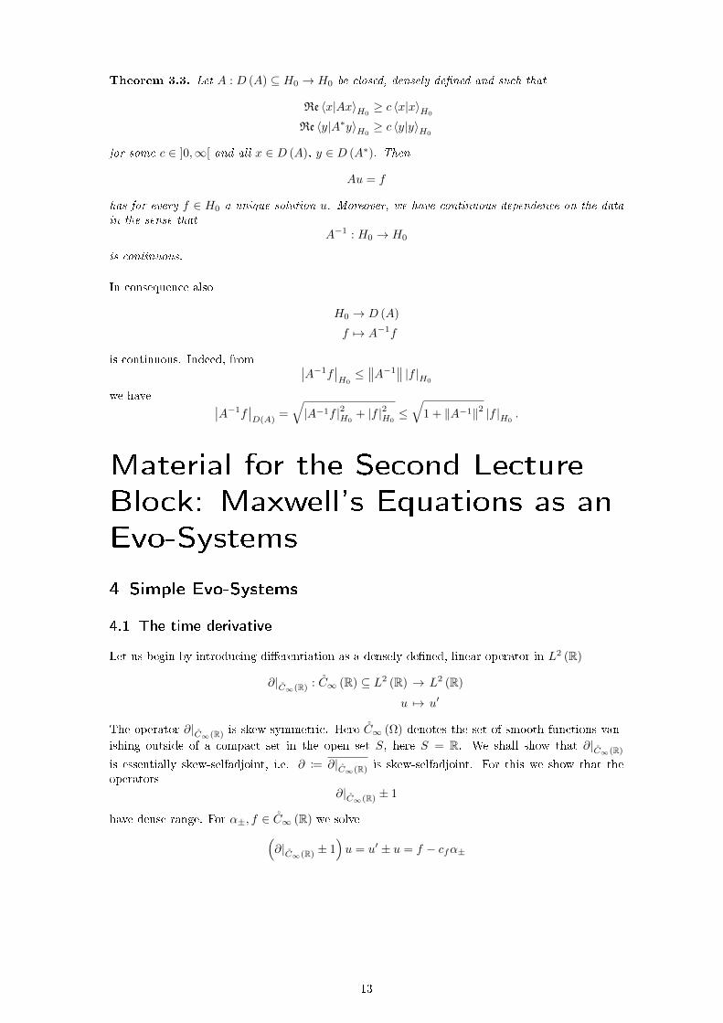
Theorem 3.3. Let A : D (A) ⊆ H0 → H0 be closed, densely dened and such that

Re 〈x|Ax〉H0≥ c 〈x|x〉H0

Re 〈y|A∗y〉H0≥ c 〈y|y〉H0

for some c ∈ ]0,∞[ and all x ∈ D (A), y ∈ D (A∗). Then

Au = f

has for every f ∈ H0 a unique solution u. Moreover, we have continuous dependence on the datain the sense that

A−1 : H0 → H0

is continuous.

In consequence also

H0 → D (A)

f 7→ A−1f

is continuous. Indeed, from ∣∣A−1f∣∣H0

≤∥∥A−1

∥∥ |f |H0

we have ∣∣A−1f∣∣D(A)

=√|A−1f |2H0

+ |f |2H0≤√1 + ‖A−1‖2 |f |H0

.

Material for the Second Lecture

Block: Maxwell's Equations as an

Evo-Systems

4 Simple Evo-Systems

4.1 The time derivative

Let us begin by introducing dierentiation as a densely dened, linear operator in L2 (R)

∂|C∞(R) : C∞ (R) ⊆ L2 (R) → L2 (R)

u 7→ u′

The operator ∂|C∞(R) is skew-symmetric. Here C∞ (Ω) denotes the set of smooth functions van-

ishing outside of a compact set in the open set S, here S = R. We shall show that ∂|C∞(R)

is essentially skew-selfadjoint, i.e. ∂ := ∂|C∞(R) is skew-selfadjoint. For this we show that theoperators

∂|C∞(R) ± 1

have dense range. For α±, f ∈ C∞ (R) we solve(∂|C∞(R) ± 1

)u = u′ ± u = f − cfα±

13

yielding

u (t) = exp (∓t)ˆ t

−∞exp (±s) (f (s)− cfα± (s)) ds

as a possible solution. To ensure that u ∈ C∞ (R) we choose α± ∈ C∞ (R) such that

ˆ ∞

−∞exp (±s) α± (s) ds = 1

and

cf :=

ˆ ∞

−∞exp (±s) f (s) ds.

Then we have for v ∈ [0](∂|C∞(R) ± 1

)∗⟨v|(∂0|C∞(R) ± 1

)u⟩0,0

= 0

for all v ∈ C∞ (R). In particular,〈v|f − cfα±〉0,0 = 0

for all f ∈ C∞ (R). It follows

〈v|f〉0,0 = 〈v|α±〉0,0 cf =

ˆ ∞

−∞〈v|α±〉0,0 exp (±s) f (s) ds

ˆ ∞

−∞v (s) f (s) ds =

ˆ ∞

−∞〈v|α±〉0,0 exp (±s) f (s) ds

=

ˆ ∞

−∞〈α±|v〉0,0 exp (±s) f (s) ds.

Thus,v = 〈α±|v〉0,0 exp (± · )

in L2,loc (R). Since exp (± · ) 6∈ L2 (R) and by assumption v ∈ L2 (R) we must have

〈α±|v〉0,0 = 0

and so v = 0. I.e.

0 = [0](∂|C∞(R) ± 1

)∗and so

(∂|C∞(R) ± 1

) [C∞ (R)

]dense in L2 (R). Thus,

(∂|C∞(R) ± 1

)−1

is a densely dened,

continuous linear operator and with the closure ∂ of ∂|C∞(R) we have(∂|C∞(R) ± 1

)−1

= (∂ ± 1)−1

: L2 (R) → L2 (R)

and so, that the operators ∂ ± 1 are onto. The skew-selfadjointness of ∂ follows.

By unitary congruence we have

exp (ρm) ∂|C∞(R) exp (−ρm) = ∂|C∞(R) − ρ

essentially skew-selfadjoint in Hρ,0 (R) = exp (ρm)[L2 (R)

]. Consequently

∂|C∞(R) =(∂|C∞(R) − ρ

)+ ρ

14

is essentially normal and so ∂0,ρ := ∂|C∞(R)Hρ,0(R)⊕Hρ,0(R)

normal with

Im ∂0,ρ =1

i∂|C∞(R) − ρ

Hρ,0(R)⊕Hρ,0(R)

andRe ∂0,ρ = ρ.

As a matter of jargon we shall write ∂0 instead of ∂0,ρ if ρ is clear from the context. Although inthe one-dimensional case the index 0 is not really needed, we use this notation to underscore that∂0 will serve as our realization of the time-derivative. For

ρ ∈ ]0,∞[ we nd12 withf (t) := 〈u (t) | u (t)〉C exp (−2ρt)

that

1

2|u (a)|2C exp (−2ρa) =

1

2

ˆ a

−∞f ′ (t) dt,

=

ˆ a

−∞Re 〈u (t) | ∂0u (t)〉C exp (−2ρt) dt− ρ

ˆ a

−∞|u (t)|2C exp (−2ρt) dt,

= Re⟨u|χ

]−∞,a]∂0u⟩ρ,0

− ρ⟨χ

]−∞,a]u|χ

]−∞,a]u⟩ρ,0, a ∈ R,

or

Re⟨u|χ

]−∞,a]∂0u⟩ρ,0

= ρ⟨χ

]−∞,a]u|χ

]−∞,a]u⟩ρ,0

+1

2|u (a)|2C exp (−2ρa) ,

≥ ρ⟨χ

]−∞,a]u|χ

]−∞,a]u⟩ρ,0, a ∈ R,

which shows a property that we would expect from time-dierentiation, its inverse ∂−10 shows the

property of causality. Indeed,

Re⟨u|χ

]−∞,a]∂0u⟩ρ,0

≥ ρ0⟨χ

]−∞,a]u|χ

]−∞,a]u⟩ρ,0

for all a ∈ R and all ρ ∈ [ρ0,∞[ shows that if f = 0 on an interval ]−∞, a] then so is ∂−10 f . This

property can also be expressed in the form

χ]−∞,a]

∂−10

(1− χ

]−∞,a]

)= 0

or

χ]−∞,a]

∂−10 = χ

]−∞,a]∂−10 χ

]−∞,a]

for all a ∈ R.

4.2 A Hilbert space perspective on ordinary dierential equations.

As an aside, we notice that the above suggests a Hilbert space theory for ordinary dierentialequations, which we explore for a moment. Indeed, assuming henceforth the forward causal caseof ρ ∈ ]0,∞[ , we have

Re ∂0 = ρ

and so ∣∣∂−10 f

∣∣ρ,0

≤ 1

ρ|f |ρ,0

12It is〈z| ζ〉C = zζ

for z, ζ ∈ C.

15

or 13 ∥∥∂−10

∥∥ ≤ 1

ρ.

Remark 4.1. We note that the norm in Hρ,0 (R) is a Hilbert space variant of the Morgensternnorm, [9]. Based on the knowledge of the fundamental solution χ

[0,∞[associated with ∂0 we have

on L∞,loc-functions f with

supexp (−ρt) |f (t)|

∣∣ t ∈ R<∞,

i.e. on L∞,ρ (R) := exp (ρm) [L∞ (R)], that

∂−10 = χ

[0,∞[∗ .

Indeed, noting that∣∣∣∣exp (−ρt)ˆ t

−∞f (s) ds

∣∣∣∣ ≤ ∣∣∣∣exp (−ρt)ˆ t

−∞exp (ρs) exp (−ρs) |f (s)| ds

∣∣∣∣ ,≤∣∣∣∣exp (−ρt)ˆ t

−∞exp (ρs) ds

∣∣∣∣ |f |L∞,ρ(R) =1

ρ|f |L∞,ρ(R)

we see that (∂−10 f

)(t) =

ˆ ∞

−∞χ

[0,∞[(t− s) f (s) ds

=

ˆ t

−∞f (s) ds

and ∣∣∂−10 f

∣∣L∞,ρ(R) ≤

1

ρ|f |L∞,ρ(R) .

Similarly for the subspace

BCρ ([0,∞[) := exp (ρm) [BC ([0,∞[)] ⊆ L∞,ρ (R) ,

which is classically of particular interest (classical Morgenstern norm). Note that due to forwardcausality ∂−1

0 [BCρ ([0,∞[)] ⊆ BCρ ([0,∞[).

All this can be lifted to the Hilbert-space-valued situation just by changing norms. In particularwe nd the following result.

Theorem 4.2. Let H be a Hilbert space and f a function with D (f) dense in Hρ,0 (R,H) andextending Lipschitz-continuously to mappings fρ : Hρ,0 (R,H) → Hρ,0 (R,H) for all ρ ∈ [ρ0,∞[and some ρ0 ∈ ]0,∞[ with a uniformly bounded Lipschitz-constant, i.e. there is a constantL ∈ ]0,∞[ with

|fρ|Lip ≤ L

for all ρ ∈ ]ρ0,∞[ . Then, for ρ > max ρ0, L there is a unique solution uρ in the Banach spaceHρ,0 (R,H) such that

∂0,ρuρ = fρ (uρ) .

Proof. First we realize that∣∣∂−10 fρ (u)− ∂−1

0 fρ (v)∣∣ρ,0,0

≤ 1

ρ|fρ|Lip |u− v|ρ,0,0

≤ 1

ρL |u− v|ρ,0,0

13Indeed, one can even conrm that∥∥∥∂−1

0

∥∥∥ = 1ρ

.

16

for all ρ ∈ [ρ0,∞[ . So, if ρ is also larger than L we have a contraction and by Banach's xedpoint theorem existence and uniqueness of a uρ with

uρ = ∂−10,ρfρ (uρ)

follows. This is equivalent to solving the above ode.

To really be able to think about ∂0 as time-dierentiation here we would have to assume addition-ally that f is causal, i.e. guided by the above observation on causality of the linear operator ∂−1

0 ,we assume that

χ]−∞,a]

f (u) = χ]−∞,a]

f(χ

]−∞,a]u)

(1)

for all a ∈ R and u ∈ D (f). This assumes implicitly that χ]−∞,a]

[D (f)] ⊆ D (f). Then we havethat the solution is essentially independent of ρ!

Theorem 4.3. Let f be as in the previous theorem with the additional property (1). If

uρk= ∂−1

0,ρkfρk

(uρk) , k = 1, 2,

for ρ1, ρ2 ∈ [ρ0,∞[ then

uρ1= uρ2

∈ Hρ1,0,0 (R,H) ∩Hρ2,0,0 (R,H) .

Proof. Due to causality, which carries over to fρk, k = 1, 2, we have

χ]−∞,a]

uρk= χ

]−∞,a]∂−10,ρk

χ]−∞,a]

fρk

(χ

]−∞,a]uρk

)= χ

]−∞,a]∂−10,ρk

fρk

(χ

]−∞,a]uρk

)and we have

χ]−∞,a]

uρ1 , χ]−∞,a]uρ2 ∈ Hminρ1,ρ2,0,0 (R,H) .

Indeed,∣∣χ]−∞,a]

u∣∣2ρk,0,0

=

ˆR

∣∣χ]−∞,a]

(t)u (t)∣∣2Hexp (−2ρkt) dt

=

ˆ a

−∞|u (t)|2H exp (−2ρkt) dt

= exp (−2ρka)

ˆ a

−∞|u (t)|2H exp (−2ρk (t− a)) dt

≤ exp (−2ρka)

ˆ a

−∞|u (t)|2H exp (−2max ρ1, ρ2 (t− a)) dt

≤ exp (2 (max ρ1, ρ2 −min ρ1, ρ2) a)ˆ a

−∞|u (t)|2H exp (−2max ρ1, ρ2 t) dt

As a consequence we ndfρ1

(χ

]−∞,a]u)= fρ2

(χ

]−∞,a]u)

for u ∈ Hρ1,0,0 (R,H) ∩ Hρ2,0,0 (R,H). Indeed, we have for a sequence x = (xk)k in D (f) con-verging to u ∈ Hminρ1,ρ2,0,0 (R,H) that

χ]−∞,a]

xkk→∞→ χ

]−∞,a]u

in Hρ1,0,0 (R,H) and in Hρ2,0,0 (R,H). Consequently,

f(χ

]−∞,a]xk) k→∞→ fρ1

(χ

]−∞,a]u)= fρ2

(χ

]−∞,a]u).

17

The same argument works for ∂−10,ρ1

and ∂−10,ρ2

. Thus, we have

χ]−∞,a]

uρ1 = χ]−∞,a]

∂−10,ρ1

χ]−∞,a]

fρ1

(χ

]−∞,a]uρ1

)= χ

]−∞,a]∂−10,ρ2

χ]−∞,a]

fρ2

(χ

]−∞,a]uρ1

).

On the other hand, we also have

χ]−∞,a]

uρ2 = χ]−∞,a]

∂−10,ρ2

χ]−∞,a]

fρ2

(χ

]−∞,a]uρ2

).

Noting thatu 7→ χ

]−∞,a]∂−10,ρ2

χ]−∞,a]

fρ2

(χ

]−∞,a]u)

is still a contraction, we have by the uniqueness of the xed point that

χ]−∞,a]

uρ2= χ

]−∞,a]uρ1

and since a ∈ R was arbitrary we obtain as claimed that

uρ2= uρ1

.

The type of equations considered in these theorems include dierential equations with delay, see[7] for more detail and a more in depth discussion.

To implement initial conditions we are looking for a solutions u of

∂0,ρ(u− χ

]0,∞[⊗ u0

)= fρ (u) ,

where u0 ∈ H is the so-called initial value. Since this clearly amounts to looking for a solution wof

∂0,ρw = fρ (w) ,

wherefρ (w) := χ

]0,∞[fρ(w + χ

]0,∞[⊗ u0

)inherits the needed Lipschitz property from fρ. Here χ]0,∞[

⊗ u0 is dened by(χ

]0,∞[⊗ u0

)(t) = χ

]0,∞[(t) u0, t ∈ R.

The desired solution u is then given by

u := χ]0,∞[

⊗ u0 + w.

Causality of ∂−10,ρ yields that w and so u must vanish on ]−∞, 0[. So we see that initial value prob-

lems were indeed already incorporated in the above, although in a slightly dierent perspective.

This concludes our little excursion into ordinary dierential equations.

It is important to realize that ∂0 and its core properties can be lifted to the Hilbert-space-valuedcase simply by replacing the inner product of C by the inner product of H.

18

4.3 Simple material laws

With u =√M0U for some selfadjoint non-negative M0 we get from the above considerations

Re⟨U |χ

]−∞,a]∂0M0U

⟩ρ,0,0

≥ ρ⟨χ

]−∞,a]

√M0U |χ

]−∞,a]

√M0U

⟩ρ,0,0

≥ ρ0

⟨χ

]−∞,a]

√M0U |χ

]−∞,a]

√M0U

⟩ρ,0,0

= ρ0⟨χ

]−∞,a]U |M0χ]−∞,a]

U⟩ρ,0,0

, a ∈ R,

for all ρ ∈ ]ρ0,∞[. Obviously we also have

Re⟨U |χ

]−∞,a]M1U

⟩ρ,0,0

=⟨χ

]−∞,a]U |ReM1χ]−∞,a]

U⟩ρ,0,0

, a ∈ R,

for all ρ ∈ ]ρ0,∞[. Our well-posedness constraint on the so-called material law operator, in ourpresent simple case

M(∂−10

):=M0 +M1∂

−10 ,

is nowρM0 +ReM1 ≥ c0 (2)

for some c0 ∈ ]0,∞[ and all suciently large ρ ∈ ]0,∞[. If we do not want to specify theparticular constant c0 we merely write 14

ρM0 +ReM1 0

for all suciently large ρ ∈ ]0,∞[ . Note that imposing this assumption also impliesM0 selfadjoint,non-negative.

In fact, according to the above we have with (2) the estimate

Re⟨U |χ

]−∞,a](∂0M0 +M1)U

⟩ρ,0,0

≥ c0∣∣χ

]−∞,a]U∣∣2ρ,0,0

(3)

for all suciently large ρ ∈ ]0,∞[ and every U ∈ D (∂0).

14We shall write for real numbers x, yx y or y x

ifx− y ≥ c > 0

for some c ∈ R. We carry this notation over to linear operators X,Y acting in a Hilbert space H, i.e. we write

X Y or Y X,

if X,Y are selfadjoint, Y continuous and

inf 〈u| (X − Y )u〉 | u ∈ BH (0, 1) ∩D (X) 0.

19

4.4 The solution theory

Let A : D (A) ⊆ H → H be a skew-selfadjoint 15 operator. We shall use ∂0M0 +M1 + A as asimplied jargon 16 for the closure M0∂0 +M1 +A of M0∂0 +M1 +A.

Theorem 4.4. Let M0, M1 and A be as in the above. Then

(M0∂0 +M1 +A)∗=M0∂∗0 +M∗

1 −A.

Proof. It is for all u ∈ Hρ,0 (R,H) and v ∈ D (∂0) ∩D (A)

〈u| (M0∂0 +M1 +A) v〉ρ,0,0 =((M0∂0 +M1 +A)

u)(v)

=:⟨(M0∂0 +M1 +A)

u|v⟩ρ,0,0

,

where(M0∂0 +M1 +A)

: H → (D (∂0) ∩D (A))

′

denotes the dual operator of (M0∂0 +M1 +A) considered as a continuous operator from D (∂0)∩D (A) to H (here H is identied with its dual). In the sense of the Gelfand triple

D

((∂0A

))= (D (∂0) ∩D (A)) ⊆ H ⊆ (D (∂0) ∩D (A))

′= D

((∂0A

))′

,

where (D (∂0) ∩D (A)) is considered as a Hilbert space with respect to the graph norm of

(∂0A

),

we have more precisely

(M0∂0 +M1 +A) :=

((M0∂0 +M1 +A) ιD(∂0)∩D(A)

)′R−1

H ,

where RH : H ′ → H denotes the Riesz map 17, so that R−1H : H → H ′, and ιD(∂0)∩D(A) :

D (∂0) ∩D (A) → H denotes the continuous, canonical embedding of D (∂0) ∩D (A) in H, i.e.

ιD(∂0)∩D(A) (x) = x

15 The skew-selfadjointness of A is responsible for an energy balance law without spatial derivatives. If

(∂0M0 +M1 +A)u = f

then since Re 〈u|Au〉H = 0 we have (clearly at least formally)

1

2∂0 〈u|M0u〉H + 〈u|ReM1u〉H = Re 〈u|M0∂0u〉H + 〈u|ReM1u〉H = Re 〈u|f〉H .

By integration over a positive-length time-interval [τ, T ], where f vanishes, we get

1

2〈u|M0u〉H (T ) +

ˆ T

τ〈u|ReM1u〉H =

1

2〈u|M0u〉H (τ) ,

which is an energy balance law in comparison to the initial energy 12〈u|M0u〉H (τ) at time τ . If ReM1 = 0,

we have indeed conservation of energy

1

2〈u|M0u〉H (T ) =

1

2〈u|M0u〉H (τ) .

We have set phrases like energy balance and energy in inverted commas, since from a mathematicalperspective to introduce the concept of energy is inappropriate and unnecessary. Following common practice,we use those terms merely as jargon.

16There is a deeper reason for this jargon . If the application of ∂0 and A is generalized in a distributional sense by re-using the notation ∂0 for the dual of its adjoint

(∂∗0

)and A for the negative of its dual A (this notation

of the dual assumes implicitly that we identify Hρ,0 (R, H) with its dual), we have indeed M0∂0 +M1 +A ⊆M0∂0 + M1 + A ⊆ ∂0M0 + M1 + A. To keep matters simple, we will not inspect this generalization processfurther, compare, however, [15], chapter 8.

17As a matter of convenience we chose the denition of the linear structure of H′ so that the Riesz map becomeslinear.

20

for x ∈ D (∂0)∩D (A). Note that ιD(∂0)∩D(A) is the canonical embedding of H in (D (∂0) ∩D (A))′

in the sense of the above Gelfand triple, which is actually the justication to use the inclusionsigns.

If now (M0∂0 +M1 +A)u ∈ H then by denition we have

(M0∂0 +M1 +A)∗u := (M0∂0 +M1 +A)

u.

With v replaced by (1 + ε∂0)−1v we obtain⟨

(1 + ε∂∗0 )−1u| (M0∂0 +M1 +A) v

⟩ρ,0,0

=⟨u| (1 + ε∂0)

−1(M0∂0 +M1 +A) v

⟩ρ,0,0

=⟨u| (M0∂0 +M1 +A) (1 + ε∂0)

−1v⟩ρ,0,0

=⟨(M0∂0 +M1 +A)

∗u| (1 + ε∂0)

−1v⟩ρ,0,0

,

=⟨(1 + ε∂∗0)

−1(M0∂0 +M1 +A)

∗u|v⟩ρ,0,0

.

Moreover,⟨(1 + ε∂∗0 )

−1u| (M0∂0 +M1 +A) v

⟩ρ,0,0

=⟨(1 + ε∂∗0)

−1u|M0∂0v

⟩ρ,0,0

+

+⟨M∗

1 (1 + ε∂∗0)−1u|v⟩ρ,0,0

+⟨(1 + ε∂∗0)

−1u|Av

⟩ρ,0,0

,

=⟨(∂∗0M0 +M∗

1 ) (1 + ε∂∗0 )−1u|v⟩ρ,0,0

+

+⟨(1 + ε∂∗0 )

−1u|Av

⟩ρ,0,0

,

and we read o that(1 + ε∂∗0)

−1u ∈ D (A∗) = D (A)

and

−A (1 + ε∂∗0 )−1u = (1 + ε∂∗0 )

−1(M0∂0 +M1 +A)

∗u− (∂∗0M0 +M∗

1 ) (1 + ε∂∗0 )−1u.

Thus we have

(∂∗0M0 +M∗1 −A) (1 + ε∂∗0)

−1u︸ ︷︷ ︸ = (1 + ε∂∗0 )

−1(M0∂0 +M1 +A)

∗u

↓u

ε↓0+

ε→0+→ (M0∂0 +M1 +A)∗u

and sou ∈ D

(∂∗0M0 +M∗

1 −A).

Thus, we have∂∗0M0 +M∗

1 −A = (M0∂0 +M1 +A)∗.

In terms of the above simplifying jargon we may write this as

(∂0M0 +M1 +A)∗= ∂∗0M0 +M∗

1 −A.

Theorem 4.5. (Solution theory) Let A : D (A) ⊆ H → H be skew-selfadjoint and let M0,M1 becontinuous linear operators satisfying (2). Then for all suciently large ρ ∈ ]0,∞[ we have thatfor every f ∈ Hρ,0 (R,H) there is a unique solution U ∈ Hρ,0 (R,H) satisfying

(∂0M0 +M1 +A)u = f.

21

Proof. The well-posedness constraint (2) now yields

Re 〈U | (∂0M0 +M1)U〉ρ,0,0 = Re 〈U | (∂0M0 +M1 +A)U〉ρ,0,0 ≥ c0 〈U |U〉ρ,0,0

for some c0 ∈ ]0,∞[ and every U ∈ D (∂0) ∩D (A). This now carries over to the closure and theadjoint by taking limits and by using Theorem 4.4. The desired result now follows.

Theorem 4.6. (Causality) Under the assumptions of Theorem 4.5 we have

χ]−∞,a]

(∂0,ρM0 +M1 +A)−1

= χ]−∞,a]

(∂0,ρM0 +M1 +A)−1χ

]−∞,a]

for all suciently large ρ ∈ ]0,∞[ .

Proof. With (3) we have for all suciently large ρ ∈ ]0,∞[

Re⟨χ

]−∞,a]U | (∂0,ρM0 +M1 +A)U

⟩ρ,0,0

= Re⟨χ

]−∞,a]U | (∂0,ρM0 +M1)U

⟩ρ,0,0

≥ c0⟨χ

]−∞,a]U |χ

]−∞,a]U⟩ρ,0,0

rst for U ∈ D (∂0) ∩D (A) end then by a density argument

Re⟨χ

]−∞,a]U |∂0,ρM0 +M1 +AU

⟩ρ,0,0

≥ c0⟨χ

]−∞,a]U |χ

]−∞,a]U⟩ρ,0,0

for all U ∈ D(∂0,ρM0 +M1 +A

). With F := ∂0,ρM0 +M1 +AU we get∣∣∣χ]−∞,a]∂0,ρM0 +M1 +A

−1F∣∣∣ρ,0,0

∣∣χ]−∞,a]

F∣∣ρ,0,0

≥

≥ Re⟨χ

]−∞,a]∂0,ρM0 +M1 +A

−1F |F

⟩ρ,0,0

≥ c0

∣∣∣χ]−∞,a]∂0,ρM0 +M1 +A

−1F∣∣∣2ρ,0,0

and so ∣∣χ]−∞,a]

F∣∣ρ,0,0

≥ c0

∣∣∣χ]−∞,a]∂0,ρM0 +M1 +A

−1F∣∣∣ρ,0,0

for every F ∈ Hρ,0 (R,H). With F =(1− χ

]−∞,a]

)F we get

χ]−∞,a]

∂0,ρM0 +M1 +A−1 (

1− χ]−∞,a]

)F = 0

orχ

]−∞,a]∂0,ρM0 +M1 +A

−1F = χ

]−∞,a]∂0,ρM0 +M1 +A

−1χ

]−∞,a]F.

Theorem 4.7. (Independence on ρ) Under the assumptions of Theorem (4.5) we have that forsome ρ0 ∈ ]0,∞[ and all ρ1, ρ2 ∈ ]ρ0,∞[ if f ∈ Hρ1 (R,H) ∩ Hρ2 (R,H) then the respectivesolutions Uρ1 and Uρ2 of

(∂0,ρ1M0 +M1 +A)Uρ1

= f

(∂0,ρ2M0 +M1 +A)Uρ2

= f

are equal.

22

Proof. Let ϕ ∈ C∞ (R) be such that ϕ = 1 on ]−∞, a[ and ϕ = 0 on ]a+ 1,∞[ then we have

(∂0,ρ1M0 +M1 +A)ϕUρ1 = ϕf + ϕ′M0Uρ1

(∂0,ρ2M0 +M1 +A)ϕUρ2

= ϕf + ϕ′M0Uρ2

in Hρ1(R,H) and Hρ2

(R,H), respectively. We shall show that

ϕUρ1 , ϕUρ2 , f ∈ Hminρ1,ρ2 (R,H) .

Assume without loss of generality ρ2 < ρ1 and a ∈ ]0,∞[ then similar as in the ODE case

|ϕUρ1|2ρ2,0,0

=

ˆ ∞

−∞|ϕUρ1

|20 exp (−2ρ2t) dt

=

ˆ a+1

−∞|ϕ (t)Uρ1

(t)|20 exp (−2ρ2t) dt

= exp (−2ρ2 (a+ 1))

ˆ a+1

−∞|ϕ (t)Uρ1 (t)|

20 exp (−2ρ2 (t− a− 1)) dt+

≤ exp (−2ρ2 (a+ 1))

ˆ a+1

−∞|ϕ (t)Uρ1 (t)|

20 exp (−2ρ1 (t− a− 1)) dt

≤ exp (2 (ρ1 − ρ2) (a+ 1))

ˆ a+1

−∞|ϕ (t)Uρ1 (t)|

20 exp (−2ρ1t)

≤ exp (2 (ρ1 − ρ2) (a+ 1)) |ϕUρ1 |2ρ1,0,0

.

Thus we have in Hρ2(R,H)

(∂0,ρ2M0 +M1 +A)ϕ (Uρ1 − Uρ2) = ϕ′M0 (Uρ1 − Uρ2)

since the right-hand side vanishes on ]−∞, a[ we have by causality that

Uρ1= Uρ2

on ]−∞, a[ .

Since a ∈ ]0,∞[ is arbitrary the desired equality follows.

So far we have avoided more complicated material laws to keep matters elementary. The followingperturbation result, however, allows to include at least a spacious class of more involved materiallaws.

For this we rst need to sharpen our positivity assumption for the material law operator. Recallingthat

Re 〈U | (∂0,ρM0 +M1)U〉ρ,0,0 = ρ 〈U |M0U〉ρ,0,0 + 〈U |ReM1U〉ρ,0,0

we nd with the orthogonal projector PM0[H0]

onto M0 [H0]

Re 〈U | (∂0,ρM0 +M1)U〉ρ,0,0 = ρ 〈U |M0U〉ρ,0,0 + 〈U |ReM1U〉ρ,0,0= ρ

⟨PM0[H]U |M0PM0[H]U

⟩ρ,0,0

+

+⟨PM0[H]U |ReM1PM0[H]U

⟩ρ,0,0

+

+2Re⟨PM0[H]U |ReM1

(1− PM0[H]

)U⟩ρ,0,0

+

+⟨(1− PM0[H]

)U |ReM1

(1− PM0[H]

)U⟩ρ,0,0

.

23

With ιM0[H] as the canonical isometric embedding of the subspace M0 [H] into H and ι[0]M0as

the canonical isometric embedding of the null space [0]M0 ofM0 into H we have by the spectraltheorem that

PM0[H]

= ιM0[H]ι∗M0[H], 1− P

M0[H]= ι[0]M0

ι∗[0]M0.

Consequently,

Re 〈U | (∂0,ρM0 +M1)U〉ρ,0,0 = ρ⟨ι∗M0[H]U |

(ι∗M0[H]M0ιM0[H]

)ι∗M0[H]U

⟩ρ,0,0

+

+⟨ι∗M0[H]U |

(ι∗M0[H] ReM1ιM0[H]

)ι∗M0[H]U

⟩ρ,0,0

+

+2Re⟨ι∗M0[H]U |

(ι∗M0[H] ReM1ι[0]M0

)ι∗[0]M0

U⟩ρ,0,0

+

+⟨ι∗[0]M0

U |(ι∗[0]M0

ReM1ι[0]M0

)ι∗[0]M0

U⟩ρ,0,0

.

To estimate this further we assume that M0 is strictly positive denite on its range and ReM1

strictly positive denite on the null space of M0. This is, we assume

ι∗M0[H]M0ιM0[H] ≥ c1 > 0, ι∗[0]M0ReM1ι[0]M0

≥ c2 > 0. (4)

With this assumption we can estimate further

Re 〈U | (∂0,ρM0 +M1)U〉ρ,0,0 ≥

≥(ρc1 −

∥∥∥ι∗M0[H] ReM1ιM0[H]

∥∥∥) ∣∣∣ι∗M0[H]U∣∣∣2ρ,0,0

+

−21

√εc2

∥∥∥ι∗M0[H] ReM1ι[0]M0

∥∥∥ ∣∣∣ι∗M0[H]U∣∣∣ρ,0,0

√εc2

∣∣∣ι∗[0]M0U∣∣∣ρ,0,0

+

+c2

∣∣∣ι∗[0]M0U∣∣∣2ρ,0,0

and so

Re 〈U | (∂0,ρM0 +M1)U〉ρ,0,0 ≥ c3 (ρ, ε)∣∣∣PM0[H]

U∣∣∣2ρ,0,0

+ c2 (1− ε)∣∣∣(1− P

M0[H]

)U∣∣∣2ρ,0,0

. (5)

for ε ∈ ]0, 1[, where

c3 (ρ, ε) := ρc1 −∥∥∥ι∗M0[H] ReM1ιM0[H]

∥∥∥−∥∥∥ι∗M0[H] ReM1ι[0]M0

∥∥∥2εc2

.

In the last step we have used the isometry of the canonical embeddings. We read o that with

c0 := min c3 (ρ, ε) , c2 (1− ε)

we have (2) as long as ρ is suciently large, i.e. c3 (ρ, ε) > 0 or

ρ >

∥∥∥ι∗M0[H] ReM1ιM0[H]

∥∥∥c1

+

∥∥∥ι∗M0[H] ReM1ι[0]M0

∥∥∥2εc1c2

. (6)

Estimate (5) permits to rene the estimate of the solution operator. We get analogously as beforefor the solution U of

∂0,ρM0 +M1 +AU = F ∈ Hρ,0 (R,H)

24

that now∣∣∣PM0[H]U∣∣∣ρ,0,0

∣∣∣PM0[H]F∣∣∣ρ,0,0

+∣∣∣(1− P

M0[H]

)U∣∣∣ρ,0,0

∣∣∣(1− PM0[H]

)F∣∣∣ρ,0,0

≥

≥ Re 〈U |F 〉ρ,0,0 ≥

≥ c3 (ρ, ε)∣∣∣PM0[H]

U∣∣∣2ρ,0,0

+ c2 (1− ε)∣∣∣(1− P

M0[H]

)U∣∣∣2ρ,0,0

and so

2√c2ε1

∣∣∣PM0[H]U∣∣∣ρ,0,0

1

2√c2ε1

∣∣∣PM0[H]F∣∣∣ρ,0,0

+

+ 2√c2ε1

∣∣∣(1− PM0[H]

)U∣∣∣ρ,0,0

1

2√c2ε1

∣∣∣(1− PM0[H]

)F∣∣∣ρ,0,0

≥ c3 (ρ, ε)∣∣∣PM0[H]

U∣∣∣2ρ,0,0

+ c2 (1− ε)∣∣∣(1− P

M0[H]

)U∣∣∣2ρ,0,0

yielding

1

4c2ε1|F |2ρ,0,0 ≥ (c3 (ρ, ε)− c2ε1)

∣∣∣PM0[H]U∣∣∣2ρ,0,0

+ c2 (1− ε− ε1)∣∣∣(1− P

M0[H]

)U∣∣∣2ρ,0,0

.

For ε1 := 1−ε2 this yields

|F |2ρ,0,0 ≥ 2c2 (1− ε) (2c3 (ρ)− c2 (1− ε))∣∣∣PM0[H]

U∣∣∣2ρ,0,0

+

+(c2 (1− ε))2∣∣∣(1− P

M0[H]

)U∣∣∣2ρ,0,0

,

where now

ρ >

∥∥∥ι∗M0[H] ReM1ιM0[H]

∥∥∥c1

+

∥∥∥ι∗M0[H] ReM1ι[0]M0

∥∥∥2εc1c2

+c2c1

1− ε

2. (7)

We are now able to show the following perturbation result.

Theorem 4.8. Let A be skew-selfadjoint in H and let M0, M1 satisfy assumption (5). Moreover,let M2 : Hρ,0 (R,H) → Hρ,0 (R,H) satisfy a Lipschitz condition

|M2 (V0)−M2 (V1)|2ρ,0,0 ≤ L20

∣∣∣PM0[H]V0 − P

M0[H]V1

∣∣∣2ρ,0,0

+

+L21

∣∣∣(1− PM0[H]

)V0 −

(1− P

M0[H]

)V1

∣∣∣2ρ,0,0

for all suciently large ρ ∈ ]0,∞[ and every U ∈ Hρ,0 (R,H) for some constants L0, L1 ∈ ]0,∞[and L1 < c2. Then we have that the problem to nd a solution U ∈ Hρ,0 (R,H) satisfying

∂0,ρM0 +M1 +M2 ( · ) +AU = F

for a given right-hand side F ∈ Hρ,0 (R,H) is uniquely solvable as long as ρ ∈ ]0,∞[ is sucientlylarge. Moreover, we have continuous dependence on the data in the sense that the Lipschitz semi-norm of the solution operator is bounded, i.e.∥∥∥∂0,ρM0 +M1 +M2 ( · ) +A

−1∥∥∥Lip

<∞.

Furthermore, if M2 is causal then also

∂0,ρM0 +M1 +M2 ( · ) +A−1

=(1− ∂0,ρM0 +M1 +A

−1M2 ( · )

)−1

(8)

is causal.

25

Proof. Consider (5) for the dierence U of solutions of

∂0,ρM0 +M1 +AUk = Fk

withFk = F −M2 (Vk) , k = 0, 1.

Then we obtain

L20

∣∣∣PM0[H]V0 − P

M0[H]V1

∣∣∣2ρ,0,0

+ L21

∣∣∣(1− PM0[H]

)V0 −

(1− P

M0[H]

)V1

∣∣∣2ρ,0,0

≥

≥ c2 (1− ε) (2c3 (ρ)− c2 (1− ε))∣∣∣PM0[H]

U∣∣∣2ρ,0,0

+ (c2 (1− ε))2∣∣∣(1− P

M0[H]

)U∣∣∣2ρ,0,0

and so with κ∗ (ε, ρ) := max

L20

c2(1−ε)(2c3(ρ)−c2(1−ε)) ,L2

1

(c2(1−ε))2

κ∗ (ε, ρ)

(c2 (1− ε) (2c3 (ρ)− c2 (1− ε))

∣∣∣PM0[H]V0 − P

M0[H]V1

∣∣∣2ρ,0,0

+

+(c2 (1− ε))2∣∣∣(1− P

M0[H]

)V0 −

(1− P

M0[H]

)V1

∣∣∣2ρ,0,0

)≥

≥ c2 (1− ε) (2c3 (ρ)− c2 (1− ε))∣∣∣PM0[H]

U∣∣∣2ρ,0,0

+ (c2 (1− ε))2∣∣∣(1− P

M0[H]

)U∣∣∣2ρ,0,0

,

For ε ∈ ]0, 1[ suciently small and ρ ∈ ]0,∞[ suciently large we have√κ∗ (ε, ρ) < 1.

Thus, we see that we have a contraction

V 7→ ∂0,ρM0 +M1 +A−1

(F −M2 (V ))

in Hρ,0 (R,H) with respect to

U 7→√c2 (1− ε) (2c3 (ρ)− c2 (1− ε))

∣∣∣PM0[H]U∣∣∣2ρ,0,0

+ (c2 (1− ε))2∣∣∣(1− P

M0[H]

)U∣∣∣2ρ,0,0

as (equivalent) norm. The unique x point U is then a desired solution. Uniqueness of this solutionfollows from the equivalence to the x point problem. We have

∂0,ρM0 +M1 +AU = F −M2 (U)

and soU = ∂0,ρM0 +M1 +A

−1(F −M2 (U)) .

This implies (8) and for for dierent data Fk, k = 0, 1, we have

Uk = ∂0,ρM0 +M1 +A−1

(Fk −M2 (Uk))

and so

|U0 − U1|ρ,0,0 =

+∣∣∣∂0,ρM0 +M1 +M2 ( · ) +A

−1F0 − ∂0,ρM0 +M1 +M2 ( · ) +A

−1F1

∣∣∣ρ,0,0

≤

≤∥∥∥∂0,ρM0 +M1 +A

−1∥∥∥ |F0 − F1|ρ,0,0 +

+∣∣∣∂0,ρM0 +M1 +A

−1M2 (Uk)− ∂0,ρM0 +M1 +A

−1M2 (Uk)

∣∣∣ρ,0,0

,

≤∥∥∥∂0,ρM0 +M1 +A

−1∥∥∥ |F0 − F1|ρ,0,0 +

+∣∣∣∂0,ρM0 +M1 +A

−1M2 ( · )

∣∣∣Lip

|U0 − U1|ρ,0,0 ,

26

from which ∣∣∣∂0,ρM0 +M1 +M2 ( · ) +A−1F0 − ∂0,ρM0 +M1 +M2 ( · ) +A

−1F1

∣∣∣ρ,0,0

≤

≤

∥∥∥∂0,ρM0 +M1 +A−1∥∥∥

1−∥∥∥∂0,ρM0 +M1 +A

−1M2 ( · )

∥∥∥Lip

|F0 − F1|ρ,0,0

and so

∥∥∥∂0,ρM0 +M1 +M2 ( · ) +A−1∥∥∥Lip

≤

∥∥∥∂0,ρM0 +M1 +A−1∥∥∥

1−∥∥∥∂0,ρM0 +M1 +A

−1M2 ( · )

∥∥∥Lip

follows.

Causality follows for a causal M2 by the causality of the x point mapping. Indeed, if F = 0on ]−∞, a[ and choosing a starting value with the same property, we see that all iterates andconsequently the limit share this property, which is nothing but the claimed causality of thesolution operator.

Typical examples for M2

(∂−10

)are delay terms, since

τ−h = exp (−h∂0)

and convolution terms

S ∗ g =√2πS

(1

i∂0

)g,

where S(1i ∂0)= LρS (m− i ρ)L−1

ρ is analytic (operator-valued) and bounded in a right half-plane,S a suitable operator-valued family (dened on some lower half-plane λ− i ρ|λ.ρ ∈ R, ρ ≥ ρ0 forsome ρ0 ∈ ]0,∞[ ).

In general, we shall speak in the context of mathematical physics problems of classical materialproperties if only selfadjoint, block-diagonal M0,M1 ,M2 occur and of metamaterials otherwise.

5 Maxwell's Equations and their Standard Initial Boundary

Value Problem.

5.1 Some spaces and operators.

Let ˚curl , div , ˚grad denote the L2 (Ω)-closure of the dierential operator matrices

0 −∂3 ∂2∂3 0 −∂1−∂2 ∂1 0

,(∂1 ∂2 ∂3

),

∂1∂2∂3

, initially dened for smooth vector elds or smooth functions with compact

support in the underlying domain Ω, respectively, which for our purposes can be any open set, sinceboundary trace results and compact embedding results are not required for basic well-posednessconsiderations. The operator curl , − grad , −div are then dened as their respective L2 (Ω)-adjoint.

27

Thus,

˚curl : D(

˚curl)⊆ L2

(Ω,C3

)→ L2

(Ω,C3

),

div : D(div)⊆ L2

(Ω,C3

)→ L2 (Ω,C) ,

˚grad : D(

˚grad)⊆ L2 (Ω,C) → L2

(Ω,C3

),

curl : D (curl ) ⊆ L2(Ω,C3

)→ L2

(Ω,C3

),

grad : D (grad ) ⊆ L2 (Ω,C) → L2(Ω,C3

),

div : D (div ) ⊆ L2(Ω,C3

)→ L2 (Ω,C) .

The denitions imply

div ˚curl = 0,

˚curl ˚grad = 0,

div curl = 0,

curl grad = 0

on D(

˚curl), D

(˚grad), D (curl ), D (grad ), respectively. This is a consequence of the orthogonal

decompositions, sometimes called Helmholtz or Helmholtz-Weyl decompositions,

L2(Ω,C3

)= grad [L2 (Ω,C)]⊕HN ⊕ ˚curl [L2 (Ω,C3)],

L2(Ω,C3

)= ˚grad [L2 (Ω,C)]⊕HD ⊕ curl [L2 (Ω,C3)],

where

HN =H ∈ L2

(Ω,C3

)| curl H = 0, divH = 0

,

HD =E ∈ L2

(Ω,C3

)| ˚curlE = 0, div E = 0

,

are the spaces of harmonic Neumann and Dirichlet elds, respectively. Their dimension is relatedto the topological properties of the underlying domain Ω. Under fairly general assumptions onthe boundary dimHN corresponds to the topological genus (number of handles) and 1 + dimHD

to the number of connected components of the boundary of Ω.

5.2 The Maxwell-Gibbs-Heaviside equations.

According to the Gibbs-Heaviside vector calculus the system of Maxwell's equations can be re-written and simplied to

∂0εE − curl H = −J∂0µH + curl E = K

We omit the superuous divergence constraints. Adding in Ohm's law

J = Jext + Jint, Jint = σE.

28

we get

∂0εE + σE − curl H = −Jext∂0µH + ˚curlE = K.

Imposing the standard electric boundary condition we obtain a system in standard form(∂0

(ε 00 µ

)+

(σ 00 0

)+

(0 − curl˚curl 0

))(EH

)=

(−JextK

).

Note that

(0 − curl˚curl 0

)is skew-selfadjoint in H = L2

(Ω,C3 ⊕ C3

)= L2

(Ω,C6

)= L2 (Ω,C)6

( 6-vector form of Maxwell's equations).

Due to div curl = 0 the usually included divergence conditions are redundant! They are indeedsuperuous and merely serve to impose constraints on the data:

div εE = −div(∂−10 Jext + σ∂−1

0 E)=: q (charge density),

divµH = div ∂−10 K (commonly assumed to vanish).

Remark 5.1. Right-hand side of Faraday's law of induction is (not) zero. The system

∂0εE + σE − curl H = −Jext∂0µH + ˚curlE = K

can under suitable assumptions be transformed to

∂0εE + σE − curl(H − ∂−1

0 µ−1K)= −Jext + ∂−1

0 curl µ−1K

∂0(µ(H − ∂−1

0 µ−1K))

+ ˚curlE = 0

or(∂0

(ε 00 µ

)+

(σ 00 0

)+

(0 − curl˚curl 0

))(E

H − µ−1∂−10 K

)=

(−Jext + curl µ−1∂−1

0 K0

).

In the context of Maxwell's equations we require

ρε+Reσ, µ 0 (9)

for well-posedness and causality. The case ε = 0 brings us back to pre-Maxwell times! If ε vanishes(globally or locally (air-iron transmission)) one speaks of the eddy current problem.

If (9) is true since M0 is strictly positive denite, i.e. ε, µ 0, we can transform the systemcongruently to obtain M0 = 1.

∂0

(ε 00 µ

)(EH

)+

(σ 00 0

)(EH

)+

(0 − curl˚curl 0

)(EH

)=

(−JextK

)(ε 00 µ

)1/2(∂0

(ε 00 µ

)1/2

+

(ε 00 µ

)−1/2(σ 00 0

)+

(ε 00 µ

)−1/2(0 − curl˚curl 0

))(EH

)=

(−JextK

)

∂0

(ε1/2Eµ1/2H

)+

(ε 00 µ

)−1/2(σ 00 0

)(ε 00 µ

)−1/2(ε1/2Eµ1/2H

)+

+

(ε 00 µ

)−1/2(0 − curl˚curl 0

)(ε 00 µ

)−1/2(ε1/2Eµ1/2H

)=

(−ε−1/2Jextµ−1/2K

)

29

and so (∂0 +

(ε 00 µ

)−1/2(σ 00 0

)(ε 00 µ

)−1/2

+Aε,µ

)(ε1/2Eµ1/2H

)=

(−ε−1/2Jextµ−1/2K

)with

Aε,µ :=

(ε 00 µ

)−1/2(0 − curl˚curl 0

)(ε 00 µ

)−1/2

=

(0 −ε−1/2 curl µ−1/2

µ−1/2 ˚curl ε−1/2 0

)skew-selfadjoint by congruence, M0 = 1, M2 = 0 and

M1 =

(ε 00 µ

)−1/2(σ 00 0

)(ε 00 µ

)−1/2

inherits selfadjointness and non-negativity) by congruence if this is assumed of σ.

5.3 The Maxwell-Gibbs-Heaviside equations in complex notation.

Let us consider the classical Maxwell caseM1 =M2 = 0, i.e. σ = 0, and, moreover, let for now ε, µjust be positive real numbers. In this case one nds occasionally a complex version of Maxwell'sequations, where E functions as real part and H as imaginary part. First we observe that underour assumptions we have

Aε,µ =

(0 − 1√

εµ curl1√εµ

˚curl 0

).

Assuming now that˚curl = curl

we see

Aε,µ =

(0 − 1√

εµ curl1√εµ curl 0

)=

(0 −11 0

)1

√εµ

curl

= i c curl

where c := 1√εµ is the velocity of light. Maxwell's equations reduce to just one equation

(∂0 + i c curl ) (E + iH) = −J + iK.

Since curl rarely equals ˚curl this is of limited use.

Remark 5.2. If : curl is equipped with a boundary condition yielding a selfadjointness realization

curl of curl this construction can also be done.

There is however an alternative which works for general ε, µ. First we note that we may reduce

30

the system to the closure of the range R (Aε,µ) of Aε,µ, i.e. we consider

ι∗R(Aε,µ)

Aε,µιR(Aε,µ)=

= ι∗R(Aε,µ)

(0 −ε−1/2 curl µ−1/2

µ−1/2 ˚curl ε−1/2 0

)ιR(Aε,µ)

=

ι∗ε−1/2R(curl )

0

0 ι∗µ−1/2R

(˚curl

)( 0 −ε−1/2 curl µ−1/2

µ−1/2 ˚curl ε−1/2 0

)( ιε−1/2R(curl )

0

0 ιµ−1/2R

(˚curl

))

=

0 −ι∗ε−1/2R(curl )

ε−1/2 curl µ−1/2ιµ−1/2R

(˚curl

)ι∗µ−1/2R

(˚curl

)µ−1/2 ˚curl ε−1/2ιε−1/2R(curl )

0

.

Since ι∗N(Aε,µ)Aε,µιN(Aε,µ) = 0 the complementary part is just an ordinary dierential equation in

H. The Maxwell system

(∂0 +Aε,µ)

(ε1/2Eµ1/2H

)=

(−ε−1/2Jextµ−1/2K

)reduces via the congruence(

ι∗R(Aε,µ)

ι∗N(Aε,µ)

)(∂0 +Aε,µ)

(ιR(Aε,µ)

ιN(Aε,µ)

)= ∂0 +

(ι∗R(Aε,µ)

Aε,µιR(Aε,µ)0

0 0

)

to (∂0 + ι∗

R(Aε,µ)Aε,µιR(Aε,µ)

)ι∗R(Aε,µ)

(ε1/2Eµ1/2H

)= ι∗

R(Aε,µ)

(−ε−1/2Jextµ−1/2K

), (10)

whereas the remaining part simply yields

ι∗N(Aε,µ)

(ε1/2Eµ1/2H

)= ∂−1

0 ι∗N(Aε,µ)

(−ε−1/2Jextµ−1/2K

).

It is worth noting that with (ε1/2e

µ1/2h

):= ι∗

R(Aε,µ)

(ε1/2Eµ1/2H

)we automatically have

div εe = div µh = 0,

which sheds again light on the redundancy of any divergence conditions.

To discuss the reduced Maxwell type equation we recall the polar decomposition:

By so-called polar decomposition we can factorize

ι∗R(A)

A : D (A) ⊆ H0 → R (A)

asι∗R(A)

A = Uι∗R(A∗)

|A| ,

whereU : R (A∗) → R (A)

is unitary and|A| :=

√A∗A.

31

More suggestively this is commonly written18 as

Ax = U |A|x

for all x ∈ D (A) = D (|A|).

By such a polar decomposition we have in the present case

ι∗µ−1/2R

(˚curl

)µ−1/2 ˚curl ε−1/2ιε−1/2R(curl )

= U

∣∣∣∣∣ι∗µ−1/2R(

˚curl)µ−1/2 ˚curl ε−1/2ι

ε−1/2R(curl )

∣∣∣∣∣ ,where

U : ε−1/2R (curl ) → µ−1/2R(

˚curl)

is unitary. We also have

ι∗ε−1/2R(curl )

ε−1/2 curl µ−1/2ιµ−1/2R

(˚curl

) =

∣∣∣∣∣ι∗µ−1/2R(

˚curl)µ−1/2 ˚curl ε−1/2ι

ε−1/2R(curl )

∣∣∣∣∣U∗

and so the congruence0 −

∣∣∣∣∣ι∗µ−1/2R(

˚curl)µ−1/2 ˚curl ε−1/2ι

ε−1/2R(curl )

∣∣∣∣∣∣∣∣∣∣ι∗µ−1/2R(

˚curl)µ−1/2 ˚curl ε−1/2ι

ε−1/2R(curl )

∣∣∣∣∣ 0

=

=

(1 00 U∗

) 0 −ι∗ε−1/2R(curl )

ε−1/2 curl µ−1/2ιµ−1/2R

(˚curl

)ι∗µ−1/2R

(˚curl

)µ−1/2 ˚curl ε−1/2ιε−1/2R(curl )

0

( 1 00 U

)

results. Thus (10) is unitarily congruent to∂0 +

0 −

∣∣∣∣∣ι∗µ−1/2R(

˚curl)µ−1/2 ˚curl ε−1/2ιε−1/2R(curl )

∣∣∣∣∣∣∣∣∣∣ι∗µ−1/2R(

˚curl)µ−1/2 ˚curl ε−1/2ιε−1/2R(curl )

∣∣∣∣∣ 0

(eh

)=

(−jk

),

18The point here is that functions (as right-unique binary relations) are dierent from mappings, which includethe recording of initial and terminal sets. As a trivial example we note that the identity is obviously a function,which may produce quite dierent mappings, such as

I0 : M → M

I1 : M → H

I2 : M ⊆ H → H.

If M is a proper subspace of H, then I0 is a linear bijection, whereas I1, I2 are not onto, although all areinjective. If topology comes into play matters become even more complex. Then we may have that I0, I1

are continuous but I2 is not. For example let H = `2 (N) :=(xk)k∈N ∈ CN|

∑nk=0 |xk|2 < ∞

with norm∣∣(xk)k∈N

∣∣`2(N) =

√∑nk=0 |xk|2and M the domain of m :D(m) ⊆ `2 (N) → `2 (N), the multiplication-by-the-

argument operatorm (xk)k∈N := (kxk)k∈N .

Then I2 is not continuous, since there cannot be an estimate of the form

n∑k=0

k2 |xk|2 ≤ Cn∑

k=0

|xk|2

holding in D (m).

32

where (eh

):=

(1 00 U∗

)ι∗R(Aε,µ)

(ε1/2Eµ1/2H

),

(−jk

):=

(1 00 U∗

)ι∗R(Aε,µ)

(−ε−1/2Jextµ−1/2K

).

Now, by the above construction this leads to the complex notation of Maxwell's equations inlossless anisotropic, inhomogeneous classical media(

∂0 + i

∣∣∣∣∣ι∗µ−1/2R(

˚curl)µ−1/2 ˚curl ε−1/2ι

ε−1/2R(curl )

∣∣∣∣∣)(e+ ih) = −j + i k.

5.4 The Maxwell-Gibbs-Heaviside equations in meta-materials.

The term meta-materials (beyond/after materials) is loosely used for materials which are notclassical in the above sense. As for the discussion of more complex media it is mostly sucient toconsider rational albeit operator-valued functions of ∂−1

0 , i.e. as material laws we allow for terms,which, after sucient dierentiation, lead to ordinary dierential equations possibly with delay.

Regular media: M0 selfadjoint and strictly positive denite.

Lossless media with no memory: M (2)(∂−10

)= 0, ReM1 = 0, i.e. M1 skew-selfadjoint.

∂0M0

(EH

)+M1

(EH

)+

(0 − curl˚curl 0

)(EH

)= J .

In this case we have conservation of energy, i.e. of the norm of√M0

(EH

).

Special cases for skew-selfadjoint M1 6= 0:

Chiral media: M1 =

(0 −SS 0

), S selfadjoint.

Ω-media: M1 =

(0 SS 0

), S skew-selfadjoint.

Bi-gyrotropic media: M1 =

(S 00 T

), S, T skew-selfadjoint.

Rational functions of ∂−10 with operator coecients:

(DB

)=

=M0

(∂−10

)( EH

)=M0 (0)

(EH

)+(M0

(∂−10

)−M0 (0)

)( EH

)

for M0 (0) =

(ε κ∗

κ µ

)with ε, µ selfadjoint. Here we assume that

M0

(∂−10

)=

N∏k=0

Pk

(∂−10

)Qk

(∂−10

)−1,

33

P,Q polynomials with (continuous, linear) operator coecients with

Qk (0) continuously invertible.

Recall the well-posedness assumption: M0 (0) continuous selfadjoint and

ρM0 (0) +ReM ′ (0) 0.

for all suciently large ρ ∈ ]0,∞[ . In the regular case, this amounts to having

M0 (0) =

(ε κ∗

κ µ

) 0.

Via the congruence (ε κ∗

κ µ

)!

(ε 00 µ− κ∗ε−1κ

)we have that we need

ε, µ− κε−1κ∗ 0.

Observing that µ− κε−1κ∗ 0 implies µ 0 and the congruence

µ− κε−1κ∗ ! 1− µ−1/2κε−1κ∗µ−1/2

= 1−(µ−1/2κε−1/2

)ε−1/2κ∗µ−1/2

= 1−∣∣∣ε−1/2κ∗µ−1/2

∣∣∣2we that the constraint µ − κε−1κ∗ 0 is a smallness constraint to the o-diagonal entry of theform 19 ∣∣∣ε−1/2κ∗µ−1/2

∣∣∣ 1.

5.5 Representation of the solution in terms of an ode fundamental solution(semi-group).

If M0 0 we already noticed the possibility of reducing the equation to the case M0 = 1.(∂0 +

(ε 00 µ

)−1/2

M1

(ε 00 µ

)−1/2

+

(ε 00 µ

)−1/2(0 − curl˚curl 0

)(ε 00 µ

)−1/2)(

ε1/2Eµ1/2H

)=

(−ε−1/2Jµ−1/2K

).

In this situation we have a fundamental solution available, which could indeed be obtained fromthe case M1 = 0 by a small perturbation argument. In the case M1 = 0 the fundamental solutionis given by

G0 (t)U0 =

exp

t( ε 0

0 µ

)−1/2(0 − curl˚curl 0

)(ε 0

0 µ

)−1/2U0 for t ≥ 0,

0 for t < 0.

19Recall that this just means that the numerical range of 1−∣∣ε−1/2κ∗µ−1/2

∣∣ or equivalently of 1−∣∣µ−1/2κε−1/2

∣∣is strictly positive. If ε, µ are just real numbers (as for homogeneous, isotropic material) we get

|κ∗| < √εµ = c−1,

where c is in physical terms the speed of light, which puts severe constraint onto admissible operators κ.

34

Here exp

(t

(ε 00 µ

)−1/2(0 − curl˚curl 0

)(ε 00 µ

)−1/2)

:= exp

(i t

(ε 00 µ

)−1/21i

(0 − curl˚curl 0

)(ε 00 µ

)−1/2)

can be conveniently understood within the function calculus of the selfadjoint operator

1

i

(ε 00 µ

)−1/2(0 − curl˚curl 0

)(ε 00 µ

)−1/2

yielding a unitary operator family. Under suitable assumptions on the data, a general solution of(∂0 +

(ε 00 µ

)−1/2(0 − curl˚curl 0

)(ε 00 µ

)−1/2)U = f

can the be represented as a convolution with the fundamental solution

U =

ˆ ∞

−∞G0 (t− s) f (s) ds,

=

ˆ t

−∞G0 (t− s) f (s) ds.

From such a representation we can read o temporal continuity properties of the solution. Re-placing G0 by the fundamental solution G associated with the perturbed operator(

∂0 +

(ε−1/2σε−1/2 0

0 µ

)+

(ε 00 µ

)−1/2(0 − curl˚curl 0

)(ε 00 µ

)−1/2),

implies a corresponding representation result.

5.6 Maxwell-Hertz equations.

Hertz picked up Maxwell's original idea of an observer in motion, which results in a system of theform

∂0µH + curl (E − v × µH) = K

∂0εE − curl (H + v × εE) = −J

Letting (1 −v × µ

v × ε 1

)(EH

)=:

(E

H

)we get (

1 −ε1/2v × µ1/2

µ1/2v × ε1/2 1

)(ε1/2Eµ1/2H

)=

(ε1/2E

µ1/2H

)and so, assuming that ε, µ are positive scalar-valued,(

1 ε1/2v × µ1/2

−µ1/2v × ε1/2 1

)(ε1/2E

µ1/2H

)=

=

(1 + ε1/2v × µ1/2µ1/2v × ε1/2 0

0 1 + µ1/2v × ε1/2ε1/2v × µ1/2

)(ε1/2Eµ1/2H

)=

(1−

∣∣∣vc

∣∣∣2 Pv

)(ε1/2Eµ1/2H

)=

(1 v

c×−v

c× 1

)(ε1/2E

µ1/2H

)

35

where Pv = − v|v| ×

v|v|× . For our solution framework we need to have that

(1 − v

c×vc× 1

)is

strictly positive denite. This is the case since we have the congruence(1 − v

c×vc× 1

)!

(1 0

0 1−∣∣ vc

∣∣2 Pv

)⟨u|(1−

∣∣∣vc

∣∣∣2 Pv

)u

⟩=

⟨Pvu|

(1−

∣∣∣vc

∣∣∣2)Pvu

⟩+ 〈(1− Pv)u| (1− Pv)u〉 ≥

(1−

∣∣∣vc

∣∣∣2) |u|2

if|v| < c.

We get with Pv/c = Pv = Pv/|v|

det

(1 v

c×−v

c× 1

)= det

(1 0

0 1−∣∣vc×∣∣2 )

= det

(1 0

0 1−∣∣vc

∣∣2 Pv/c

)=

(1−

∣∣∣vc

∣∣∣2)Calculating the eigenvalues we nd they are mostly 1 but(

1−∣∣∣vc

∣∣∣2 Pv/c

)x =

(1− Pv/c

)x+

(1−

∣∣∣vc

∣∣∣2)Pv/cx = λx = λ((1− Pv/c

)x+ Pv/cx

)yields

λ = 1, 1,

(1−

∣∣∣vc

∣∣∣2)and so by Cramer's rule(

1 −vc×

vc× 1

)−1

=

(1−

∣∣ vc

∣∣2)−1 (1−

∣∣vc

∣∣2)−1vc×

−(1−

∣∣vc

∣∣2)−1vc×

(1−

∣∣vc

∣∣2)−1

.

Thus we nd

∂0

(ε1/2Eµ1/2H

)+

(ε 00 µ

)−1/2(0 − curl

curl 0

)(ε 00 µ

)−1/2(ε1/2E

µ1/2H

)=

(−ε−1/2Jµ−1/2K

)

∂0

(1−

∣∣ vc

∣∣2)−1 (1−

∣∣vc

∣∣2)−1vc×

−(1−

∣∣vc

∣∣2)−1vc×

(1−

∣∣ vc

∣∣2)−1

( ε1/2E

µ1/2H

)+

+

(ε 00 µ

)−1/2(0 − curl

curl 0

)(ε 00 µ

)−1/2(ε1/2E

µ1/2H

)=

(−ε−1/2Jµ−1/2K

).

Bringing it back to standard Maxwell form (with the standard electric boundary condition)(∂0M0 +

(0 − curl˚curl 0

))(E

H

)=

(−JK

),

where

M0 =

(ε 00 µ

)1/2

(1−

∣∣ vc

∣∣2)−1 (1−

∣∣vc

∣∣2)−1vc×

−(1−

∣∣ vc

∣∣2)−1vc×

(1−

∣∣vc

∣∣2)−1

( ε 00 µ

)1/2

.

In this form we could now even let v be variable and ε, µ arbitrary strictly positive L∞-multiplicationoperators without destroying the well-posedness and causality result.

36

6 Maxwell's Equations and a Leontovich Type Boundary

Condition.

Due to the orthogonal decomposition

D (curl ) = D(

˚curl)⊕N (1 + curl curl )

and with containment inD(

˚curl)encoding vanishing of the tangential component at the boundary

in a generalized sense we may take N (1 + curl curl ) as space of tangential boundary values. Withthe canonical embedding

ιN(1+curl curl ) : N (1 + curl curl ) → D (curl )

x 7→ x

we have thatι∗N(1+curl curl ) : D (curl ) → N (1 + curl curl )

projects orthogonally on N (1 + curl curl ).

Let us consider

∂0M0 +M1 +

0 −(

curlι∗N(1+curl curl )

)∗

(curl

ι∗N(1+curl curl )

) (0 00 0

) .

The underlying Hilbert space is

H = L2(Ω,C3

)⊕(L2(Ω,C3

)⊕N (1 + curl curl )

).

Since (˚curl0

)⊆(

curlι∗N(1+curl curl )

),

we note that (curl

ι∗N(1+curl curl )

)∗

⊆(

˚curl0

)∗

=(curl 0

).

The latter yields that (curl

ι∗N(1+curl curl )

)∗(Hτ

)= curl H

for all

(Hτ

)∈ D

((curl

ι∗N(1+curl curl )

)∗). To inspect this more closely we calculate

⟨curl Φ

∣∣∣H⟩L2(Ω,C3)

+⟨ι∗N(1+curl curl )Φ

∣∣∣τ⟩N(1+curl curl )

=

=

⟨(curl

ι∗N(1+curl curl )

)Φ∣∣∣ (H

τ

)⟩L2(Ω,C3)⊕N(1+curl curl )

=

⟨Φ∣∣∣ ( curl

ι∗N(1+curl curl )

)∗(Hτ

)⟩L2(Ω,C3)

= 〈Φ| curl H〉L2(Ω,C3)

37

yielding ⟨Φ∣∣∣ curl H⟩

L2(Ω,C3)−⟨curl Φ

∣∣∣H⟩L2(Ω,C3)

=⟨Φ∣∣∣τ⟩

D(curl )

=⟨ι∗N(1+curl curl )Φ

∣∣∣τ⟩N(1+curl curl )

for all

(Hτ

)∈ D

((curl

ι∗N(1+curl curl )

)∗)and Φ ∈ D (curl ) = D

((curl

ι∗N(1+curl curl )

)). Now, since⟨

Φ∣∣∣ curl H⟩

L2(Ω,C3)−⟨curl Φ

∣∣∣H⟩L2(Ω,C3)

vanishes for Φ ∈ D(

˚curl)we may assume without loss

of generality that Φ ∈ N (1 + curl curl ) and replace H by ι∗N(1+curl curl )H. In this case we seethat⟨Φ∣∣∣ curl H⟩

L2(Ω,C3)−⟨curl Φ

∣∣∣H⟩L2(Ω,C3)

=

=1

2

(⟨Φ∣∣∣ curl ι∗N(1+curl curl )H

⟩L2(Ω,C3)

−⟨curl Φ

∣∣∣ι∗N(1+curl curl )H⟩L2(Ω,C3)

)+

− 1

2

(⟨curl curl Φ

∣∣∣ curl ι∗N(1+curl curl )H⟩L2(Ω,C3)

−⟨curl Φ

∣∣∣ curl curl ι∗N(1+curl curl )H⟩L2(Ω,C3)

)=

1

2

(⟨Φ∣∣∣ curl ι∗N(1+curl curl )H

⟩L2(Ω,C3)

+⟨curl Φ

∣∣∣ curl curl ι∗N(1+curl curl )H⟩L2(Ω,C3)

)+

− 1

2

(⟨curl Φ

∣∣∣ι∗N(1+curl curl )H⟩L2(Ω,C3)

+⟨curl curl Φ

∣∣∣ curl ι∗N(1+curl curl )H⟩L2(Ω,C3)

)=

1

2

(⟨Φ∣∣∣ curl ι∗N(1+curl curl )H

⟩N(1 curl curl )

−⟨curl Φ

∣∣∣ι∗N(1+curl curl )H⟩N(1 curl curl )

),

where we have used that Φ ∈ N (1 + curl curl ) implies curl Φ ∈ N (1 + curl curl ). Moreover, wehave that

•curl : N (1 + curl curl ) → N (1 + curl curl )

Φ 7→ curl Φ

is unitary and skew-selfadjoint. Indeed,⟨Φ∣∣∣ •curlΨ

⟩N(1+curl curl )

=⟨Φ∣∣∣ curl Ψ⟩

N(1+curl curl )

=⟨Φ∣∣∣ curl Ψ⟩

L2(Ω,C3)+⟨curl Φ

∣∣∣ curl curl Ψ⟩L2(Ω,C3)

= −⟨curl curl Φ

∣∣∣ curl Ψ⟩L2(Ω,C3)

−⟨curl Φ

∣∣∣Ψ⟩L2(Ω,C3)

= −⟨curl Φ

∣∣∣Ψ⟩N(1+curl curl )

=

⟨−

•curl Φ

∣∣∣Ψ⟩N(1+curl curl )

and so•

curl∗= −

•curl .

38

Similarly,⟨•

curl Φ∣∣∣ •curlΨ

⟩N(1+curl curl )

=⟨curl Φ

∣∣∣ curl Ψ⟩N(1+curl curl )

=⟨curl Φ

∣∣∣ curl Ψ⟩L2(Ω,C3)

+⟨curl curl Φ

∣∣∣ curl curl Ψ⟩L2(Ω,C3)

=⟨curl Φ

∣∣∣ curl Ψ⟩L2(Ω,C3)

+⟨Φ∣∣∣Ψ⟩

L2(Ω,C3)

=⟨Φ∣∣∣Ψ⟩

N(1+curl curl )

showing that•

curl is an isometry. That•

curl is onto follows since

•curl

•curl = −1.

Thus, we have that•

curl−1

= −•

curl =•

curl∗.

With this we get⟨Φ∣∣∣ curl H⟩

L2(Ω,C3)−⟨curl Φ

∣∣∣H⟩L2(Ω,C3)

=

=1

2

(⟨Φ∣∣∣ •curl ι∗N(1+curl curl )H

⟩N(1+curl curl )

−⟨

•curl Φ

∣∣∣ι∗N(1+curl curl )H

⟩N(1 curl curl )

),

=

⟨Φ∣∣∣ •curl ι∗N(1+curl curl )H

⟩N(1+curl curl )

.

By comparison ⟨Φ∣∣∣ •curl ι∗N(1+curl curl )H

⟩N(1 curl curl )

=⟨Φ∣∣∣τ⟩

N(1+curl curl )

for all Φ ∈ N (1 + curl curl ) we see that

τ =•

curl ι∗N(1+curl curl )H.

Consequently,

D

((curl

ι∗N(1+curl curl )

)∗)⊆

(H

•curl ι∗N(1+curl curl )H

)∣∣∣H ∈ D (curl )

.

Consider as a special case

M0 =

ε(0 0

)(00

) (µ 00 α

)

M1 =

σ(0 0

)(00

) (0 00 β

) .

Then, it follows (at least for regular right-hand sides F =

−J(Kh

) say F, ∂0F ∈ Hρ (R,H))

that

∂0εE + σE − curl H = −J,∂0µH + curl E = K,

∂0ατ + βτ + ι∗N(1+curl curl )E = h.

39

Inserting our nding for τ into the last equation yields

(∂0α+ β)•

curl ι∗N(1+curl curl )H + ι∗N(1+curl curl )E = h,

which is a generalized Leontovitch type boundary condition. Note that•

curl corresponds formally20 to n× in boundary trace terms. In particular, ι∗N(1+curl curl )E corresponds to −n×n×E since

ι∗N(1+curl curl )E = −•

curl•

curl ι∗N(1+curl curl )E.

Thus, the above equation generalizes the classical boundary equation

(∂0α+ β)n×H − n× n× E = h,

or (indicating taking the tangential component by a lower index t)

Et = (∂0α+ β) (Ht × n) + h,

which adds a dynamic constraint on the boundary. If preferable the role of E and H can beinterchanged, then the boundary

(∂0α+ β)•

curl ι∗N(1+curl curl )E + ι∗N(1+curl curl )H = h,

or

− (∂0α+ β) ι∗N(1+curl curl )E +•

curl ι∗N(1+curl curl )H =•

curlh.

The latter corresponds to(∂0α+ β)Et = (n×Ht)− n× h

leading to(∂0α+ β)

−1(n×Ht − n× h) = Et,

which is indeed a classical, dynamic, inhomogeneous Leontovich type boundary condition.

20This correspondence rests on the observation that

〈Φ|n×H〉L2(∂Ω) =

ˆ∂Ω

Φ · (n×H) do

= −ˆ∂Ω

n ·(Φ×H

)do

= −ˆΩdiv

(Φ×H

)dV

=⟨Φ∣∣∣ curl H⟩

L2(Ω,C3

) − ⟨curl Φ

∣∣∣H⟩L2

(Ω,C3

)=

⟨ι∗N(1+curl curl )Φ|

•curl ι∗N(1+curl curl )H

⟩N(1+curl curl )

.

If we had a boundary trace mapping

γ : N (1 + curl curl ) → L2 (∂Ω)

then

γ∗n× γ =•

curl .

However, such a boundary trace does in general not exist. To follow this reasoning, we need to modify curl to

a curl warranting a boundary trace in L2 (∂Ω). The boundary trace mapping into L2 (∂Ω) is then a mapping

γ : N(1 + curl curl

)→ L2 (∂Ω)

and so

γ∗n× γ =•

curl ,

where•

curl : N(1 + curl curl

)→ N

(1 + curl curl

).

40

7 The Extended Maxwell System

7.1 A note on classical Maxwell equations in dierential form language.

An independent strand of development is rooted in the use of alternating dierential forms forthe formulation of the Maxwell-Heaviside system. The rigorous investigation of initial boundaryvalue problems for Maxwell's equations in the alternating dierential form setting goes back toH. Weyl, [22], K. O. Friedrichs, [4]. We mention in passing that, as noticed by N. Weck, thedierential forms framework proved to be essential in showing a compact resolvent result for thespatial derivative operator of Maxwell's equations in the case of non-smooth boundaries, see [20].Such types of results were previously derived from Rellich's compact embedding result, which,however, fails to hold even for simple non-smooth boundaries such as for example a unit cube]0, 1[

3with a smaller cube [0, ε]

3, ε ∈ ]0, 1[, removed.

The so-called exterior derivative d is (we focus on the 3-dimensional Euclidean case) formally givenrecursively as

df := ∂1f dx1 + ∂2f dx

2 + ∂3f dx3

d

(∑α

aαdxα∧

):=

∑α∈1,2,3qincreasing

daα ∧ dxα∧.

In analogy to the vector-analytical case, we dene d again as the L2-closure of d dened on formswith smooth coecients having compact support. Here the Hilbert spaces L2,q (Ω) of correspond-ing q− forms ( q = 0, 1, 2, 3) can be understood as the completion of such smooth, compactlysupported q−forms with respect to the norm induced by the inner product

〈 · | · 〉L2,q(Ω) = (ω, η) 7→ˆM

ω ∧ ∗qη

where the so-called Hodge star operator ∗q is given in R3 as

∗01 = dx1 ∧ dx2 ∧ dx3 (volume element),

∗q∗3−q = 1,

∗1dxk = dxk+1 ∧ dxk+2 (k mod 3) .

We introduce d := −(d)∗

and nd by integration by parts

ˆM

d ∧ (α ∧ ∗qη) =ˆM

dα ∧ ∗qη + (−1)q−1ˆM

α ∧ d ∗q η

= 〈dα|η〉q + (−1)q−1ˆM

α ∧ ∗q−1 ∗3−q+1 d ∗q η

= 〈dα|η〉q +⟨α| (−1)

q−1 ∗3−q+1 d ∗q η⟩q−1

motivating the denition of a generalized derivative

(−1)q−1 ∗3−q+1 d∗q := d.

Formally, it is for a 1-form E and a 2-form H

dE ' curl E,

dH ' − curl H.

41

Observing (0 d

d 0

)(EH

)=(d+ d

)(E +H)

Maxwell's equations can formally be written as(∂0M0 +M1 + d+ d

)(E +H) = −J +K.

If M0 happens to be strictly positive denite we may reformulate this as(∂0 +

√M−1

0 M1

√M−1

0 +

√M−1

0

(d+ d

)√M−1

0

)√M0 (E +H) =

√M−1

0 (−J +K) .

Material for the Third Lecture

Block: The Extended Maxwell

System

7.2 Extended Maxwell system.

Following the intrinsic logic of the dierential forms setting a functional analytical framework forinitial boundary value problems for Maxwell's equations can be embedded in an extended rstorder system on Riemannian manifolds, [14]. Considering the Euclidean free space case it turnsout that this extension formally coincides with the so-called Ohmura system.

Let initially M0 = 1, M1 = 0. We note

dE ' curl E

dE ' div E

dH ' − curl H

dH ' div H

df ' grad f

dψ ' grad ψ

and extend the Maxwell operator in a natural way to alternating dierential forms of all degrees0 d 0 0

d 0 d 0

0 d 0 d

0 0 d 0

ϕEHψ

=(d+ d

) (ϕ(0) + E(1) +H(2) + ψ(3)

).

We also note the unitary congruence0 d 0 0

d 0 d 0

0 d 0 d

0 0 d 0

ϕEHψ

!

0 0 0 d

0 0 d d0 d 0 0

d d 0 0

ψ(3)

E(1)

ϕ(0)

H(2)

bringing the operator matrix into standard form(

0 −C∗

C 0

)

42

and allowing the decomposition0 0 0 d

0 0 d d0 d 0 0

d d 0 0

=

0 0 0 00 0 0 d0 0 0 0

0 d 0 0

+

0 0 0 d0 0 0 00 0 0 0d 0 0 0

+

0 0 0 0

0 0 d 00 d 0 00 0 0 0

into commuting skew-selfadjoint summands, which indeed annihilate each other.

For variable coecients

0 0 0 dµ0 0 0 00 0 0 0dα 0 0 0

+

0 0 0 0

0 0 dβ 00 dε 0 00 0 0 0

=

0 0 0 d0 0 0 00 0 0 0d 0 0 0

+

0 0 0 0

0 0 d 00 d 0 00 0 0 0

α 0 0 00 ε 0 00 0 β 00 0 0 µ

we write the extended Maxwell system as∂0 +

α 0 0 00 ε 0 00 0 β 00 0 0 µ

−1

0 0 0 00 0 0 d0 0 0 0

0 d 0 0

+

0 0 0 d0 0 0 00 0 0 0d 0 0 0

+

0 0 0 0

0 0 d 00 d 0 00 0 0 0

α 0 0 00 ε 0 00 0 β 00 0 0 µ

ψEϕH

= F.

In the Maxwell case

F =

α 0 0 00 ε 0 00 0 β 00 0 0 µ

−1

−d∂−10 J

−Jd∂−1

0 KK

,

It is preferable to write the system again in the more symmetric form∂0 +√E−1

0 0 0 00 0 0 d0 0 0 0

0 d 0 0

√E−1 +

√E

0 0 0 d0 0 0 00 0 0 0d 0 0 0

+

0 0 0 0

0 0 d 00 d 0 00 0 0 0

√

E

√

E

ψEϕH

=

√E−1F

with

E =

α 0 0 00 ε 0 00 0 β 00 0 0 µ

=M0

or even a more general E .

In vector analytical form, compare [16], this is

(∂0 +AE,XMax)

√E

−ψEϕH

=

√E−1F,

where

AE,XMax :=√E−1

0 0 0 00 0 0 − curl0 0 0 0

0 ˚curl 0 0

√E−1+

√E

0 0 0 −div0 0 0 00 0 0 0

− grad 0 0 0

+

0 0 0 0

0 0 ˚grad 00 div 0 00 0 0 0

√

E .

43

In the case of the classical Maxwell's equations (i.e. E =

α 0 0 00 ε 0 00 0 β 00 0 0 µ

) we have

√E−1F =

−α−1/2div ∂−1

0 J−ε−1/2J

−β−1/2 div ∂−10 K

µ−1/2K

from which ϕ = ψ = 0 can be concluded (see the factorization below).

Historical comments: This has been discovered and rediscovered within the logic and in the lan-guage of quaternions. It also appears in Dirac's work in the discussion of magnetic monopoles andan associated symmetric construction for potentials , which really just means solving

(∂0 −AE,XMax)P =

√E

0E0H

,

(∂20 −A2

E,XMax

)P = (∂0 +AE,XMax) (∂0 −AE,XMax)P = (∂0 +AE,XMax)

√E

0E0H

,

=

−α−1/2div ∂−1

0 J−ε−1/2J

−β−1/2 div ∂−10 K

µ−1/2K

.

In Dirac's case this is considered for constant scalar coecients with α = β = 1.

The extended Maxwell system amounts to a specic coupling of acoustic equations with Maxwell'sequations, [13]:

AMax =

0 0 0 00 0 0 − curl0 0 0 0

0 ˚curl 0 0

ADac :=

0 0 0 0

0 0 ˚grad 00 div 0 00 0 0 0

,

ANac :=

0 0 0 −div0 0 0 00 0 0 0

− grad 0 0 0

,

Aac :=

0 0 0 −div

0 0 ˚grad 00 div 0 0

− grad 0 0 0

= ADac +ANac.

With these skew-selfadjoint operators the extended Maxwell system is given by

44

(∂0 +

√E−1AMax

√E−1 +

√EAac

√E)V = F ,

where V =√EU , and E is selfadjoint, bounded and strictly positive denite (taking over the role

of M0 in the previous section) and for equivalence to the original Maxwell system we would have

to choose F =√E−1F + ∂−1

0

√EAacF .

The extended Maxwell system(∂0 +AE,XMax)U = F ,

where

AE,XMax =√E−1AMax

√E−1 +

√EAac

√E

is skew-selfajoint in L2 (Ω)8and the equation is again of the general form discussed in the intro-

duction.

Actually: no coupling between√E−1AMax

√E−1 and

√EAac

√E occurring!

√E−1AMax

√E−1

√EAac

√E =

√E−1AMaxAac

√E = 0,

√EAac

√E√E−1AMax

√E−1 =

√EAacAMax

√E−1 = 0,

on D(Aac

√E)and on D

(AMax

√E−1

), respectively. In particular we have

D (AE,XMax) = D(AMax

√E−1

)∩D

(√EAac

√E).

It is still useful to consider this extended Maxwell system e.g. for numerical purposes, see [18, 21],or low frequency limits [11, 12, 13], since the spatial operator is now a dierential operator ofelliptic type, yielding a small (e.g. a nite dimensional) null space.

From this we have that(Im ∂0,

1i

√E−1AMax

√E−1, 1

i

√EAac

√E)is a family of commuting, self-

adjoint operators.

In the framework of the associated function calculus we have that the operator on the left-handside is now a function of this family given by

(x, y, z) → i (x+ y + z) + ν.

Moreover, we have the factorization:(∂0 +

√E−1AMax

√E−1

)(∂0 +

√EAac

√E)= ∂0

(∂0 +

√E−1AMax

√E−1 +

√EAac

√E).

Thus,

∂−10

(∂0 +

√E−1AMax

√E−1

)(∂0 +

√EAac

√E)=(∂0 +

√E−1AMax

√E−1 +

√EAac

√E)

and so assuming that F is in D(Aac

√E)we get U ∈ D

(Aac

√E)and

(∂0 +

√E−1AMax

√E−1 +

√EAac

√E)U = ∂−1

0

(∂0 +

√EAac

√E)(

∂0 +√E−1AMax

√E−1

)U

= ∂−10

(∂0 +

√EAac

√E)F

=(1 + ∂−1

0

√EAac

√E)F =: G

45

equivalent to (∂0 +

√E−1AMax

√E−1

)U = F = ∂0

(∂0 +

√EAac

√E)−1

G.

This recovers and conrms our earlier observation. For a proper reduction to Maxwell's equationwe must have that here F and E are of the block matrix form

F =

0?0?

, E =

? 0 0 00 ? 0 ?0 0 ? 00 ? 0 ?

which ensures that the solution U is also of the form

U =

0E0H

,

so that by dropping rows and column containing only zeros, we recover indeed the original Maxwellsystem.

For E =

? 0 0 ?0 ? ? 00 ? ? 0? 0 0 ?

. we even have that(∂0,

√E−1AMax

√E−1 + 1,

√EADac

√E + 1,

√EANac

√E + 1

)is a family of commuting normal, continuously invertible operators. Now, since

√E−1AMax

√E−1,√

EADac

√E ,

√EANac

√E , annihilate each other pair-wise, we get the following factorization:(

∂0 +√E−1AMax

√E−1

)(∂0 +

√EADac

√E)(

∂0 +√EANac

√E)=

= ∂20

(∂0 +

√E−1AMax

√E−1 +

√EADac

√E +

√EANac

√E)

Thus,

∂−20

(∂0 +

√E−1AMax

√E−1

)(∂0 +

√EADac

√E)(

∂0 +√EANac

√E)=

=(∂0 +

√E−1AMax

√E−1 +

√EADac

√E +

√EANac

√E)

(∂0 +

√E−1AMax

√E−1 +

√EADac

√E +

√EANac

√E)U =

= ∂−20

(∂0 +

√EADac

√E)(

∂0 +√EANac

√E)(

∂0 +√E−1AMax

√E−1

)U

= ∂−20

(∂0 +

√EADac

√E)(

∂0 +√EANac

√E)F

=(1 + ∂−1

0

√EADac

√E)(

1 + ∂−10

√EANac

√E)F =: G

equivalent to(∂0 +

√E−1AMax

√E−1

)U = F = ∂0

(∂0 +

√EADac

√E)−1

∂0

(∂0 +

√EANac

√E)−1

G.

We also see that(∂0 +

(√E−1AMax

√E−1 +

√EAac

√E))(

∂0 −(√

E−1AMax

√E−1 +

√EAac

√E))

=

= ∂20 −(√

E−1AMax

√E−1 +

√EADac

√E +

√EANac

√E)2

= ∂20 −((√

E−1AMax

√E−1

)2+(√

EADac

√E)2

+(√

EANac

√E)2)

.

46

For constant scalar coecients, without loss of generality we will choose E = 1, this reducesformally to

∂20 −(A2

Max +A2Dac +A2

Nac

)= ∂20 −∆ =: , (11)

i.e. the classical wave operator (with unusual boundary conditions). This leads in the time-harmonic case to a weakly singular Green's tensor, which explains the mentioned interest fornumerical methods.

Remark 7.1.

. GEM: The linear equations of gravitation, A. Singh, [17] (quaternions!),

∂0 + (AMax +ADac +ANac)

received renewed interest in the context of modern gravito-electromagnetism (GEM),[19].

(∂0 + (AMax +ADac))U = F ∈ Hν,−∞ (R,H1 (ANac + 1)) ,

leading to

(∂0 + (AMax +ADac +ANac))U =(1 + ∂−1

0 ANac

)F.

Or conversely, if

(∂0 + (AMax +ADac +ANac))U = G

then

∂0 + (AMax +ADac)U = ∂0 (∂0 +ANac)−1G.

It may be noteworthy that in the latter case we have

∂0 (∂0 +ANac)−1G ∈ Hν,−∞ (R,H1 (ANac + 1)) .

This system makes its reappearance from a completely dierent angle in [10] and for numer-ical purposes in [1], [21], as an alternative to the fully extended Maxwell system.

. Of course we can also consider the extended system with more general material laws forexample by considering

(∂0M0 +M1 +AE,XMax)U = F.

The connection to Maxwell's equations and the acoustic equations is then, however, generallylost.

7.3 Dirac's equation

From ( 11) we see that Dirac's problem of nding a rst order factorization of the dierentialoperator of the wave equation (rather of the Klein-Gordon operator), which gave rise to thecelebrated Dirac equations [2, 3], is solved by the extended Maxwell system with E = 1. Thisobservation will now be utilized to reformulate Dirac's equation as an extended Maxwell system.

The classical Dirac equations with mass m = 1 can be given in the form

Q0(∂0, ∂) =

(∂0 + i C(∂)

C(∂) ∂0 − i

),

where

C(∂) =

(∂3 ∂1 − i ∂2

∂1 + i ∂2 −∂3

)

47

Applying the unitary congruence given by the block matrix 1√2

(+i +1i −1

)to Q0(∂0, ∂) we obtain

Q1(∂0, ∂) :=

(∂0 i − i C(∂)

i + i C(∂) ∂0

)=

= 12

(+i +1i −1

)(−i ∂0 + 1 + C(∂) −i ∂0 + 1− C(∂)

−i C(∂) + ∂0 − i −i C(∂)− ∂0 + i

)= 1

2

(+i +1i −1

)(∂0 + i C(∂)

C(∂) ∂0 − i

)(−i −i+1 −1

).

The latter may be a preferable form since Q1(∂0, ∂) has in R3 the typical Hamiltonian form ofreversibly evolutionary expressions of mathematical physics

∂0 +

(0 −W ∗

W 0

),

where here W := i + i C(∂) =

(i ∂3 + i i ∂1 + ∂2i ∂1 − ∂2 −i ∂3 + i

). To see the connection between the Dirac

equation and the extended Maxwell equation we separate real and imaginary parts 21, which yieldsthat W corresponds to

W =

0 −1− ∂3 ∂2 −∂1

1 + ∂3 0 ∂1 ∂2−∂2 −∂1 0 −1 + ∂3∂1 −∂2 1− ∂3 0

=

0 −1 0 01 0 0 00 0 0 −10 0 1 0

+

0 −∂3 ∂2 −∂1∂3 0 ∂1 ∂2−∂2 −∂1 0 ∂3∂1 −∂2 −∂3 0

.

Noting that i C(∂) =

0 −∂3 ∂2 −∂1∂3 0 ∂1 ∂2−∂2 −∂1 0 ∂3∂1 −∂2 −∂3 0

is formally L2-selfadjoint,

0 1 0 00 0 −1 00 0 0 −1−1 0 0 0

W0

0 1 0 00 0 −1 00 0 0 −1−1 0 0 0

∗

=

0 1 0 00 0 −1 00 0 0 −1−1 0 0 0

0 −∂3 ∂2 −∂1∂3 0 ∂1 ∂2−∂2 −∂1 0 ∂3∂1 −∂2 −∂3 0

0 0 0 −11 0 0 00 −1 0 00 0 −1 0

= −

0 1 0 00 0 −1 00 0 0 −1−1 0 0 0

∂3 ∂2 ∂1 00 ∂1 ∂2 ∂3∂1 0 ∂3 −∂2∂2 −∂3 0 ∂1

= −

0 ∂1 ∂2 ∂3

−∂1 0 −∂3 ∂2−∂2 ∂3 0 −∂1−∂3 −∂2 ∂1 0

=

(0 −div

grad − curl

)

21 This transition is unitary if we consider the underlying spaces as linear spaces over the eld R. This is inheritedfrom the fact that, although R is 1-dimensional as a linear space over R and C is 1-dimensional over the eld C,C considered as a linear space over the eld R is unitarily equivalent to R2, the unitary mapping being given by

R2 → C,(x, y) 7→ x+ i y.

48

and0 1 0 00 0 −1 00 0 0 −1−1 0 0 0

0 −1 0 01 0 0 00 0 0 −10 0 1 0

0 1 0 00 0 −1 00 0 0 −1−1 0 0 0

∗

=

0 1 0 00 0 −1 00 0 0 −1−1 0 0 0

0 −1 0 01 0 0 00 0 0 −10 0 1 0

0 0 0 −11 0 0 00 −1 0 00 0 −1 0

=

0 1 0 00 0 −1 00 0 0 −1−1 0 0 0

−1 0 0 00 0 0 −10 0 1 00 −1 0 0

=

0 0 0 −10 0 −1 00 1 0 01 0 0 0

we obtain the unitary congruence

0 −1 0 00 0 1 00 0 0 11 0 0 0

0 0 0 00 0 0 00 0 0 00 0 0 0

0 0 0 00 0 0 00 0 0 00 0 0 0

0 1 0 00 0 −1 00 0 0 −1−1 0 0 0

(

0 −W ∗

W 0

)

0 0 0 1−1 0 0 00 1 0 00 0 1 0

0 0 0 00 0 0 00 0 0 00 0 0 0

0 0 0 00 0 0 00 0 0 00 0 0 0

0 0 0 −11 0 0 00 −1 0 00 0 −1 0

=

0 1 0 00 0 1 00 0 0 11 0 0 0

0 0 0 00 0 0 00 0 0 00 0 0 0

0 0 0 00 0 0 00 0 0 00 0 0 0

0 0 −1 00 0 0 −1−1 0 0 00 1 0 0

(

0 −W ∗

W 0

)

0 0 0 11 0 0 00 1 0 00 0 1 0

0 0 0 00 0 0 00 0 0 00 0 0 0

0 0 0 00 0 0 00 0 0 00 0 0 0

0 0 −1 00 0 0 1−1 0 0 00 −1 0 0

=

0

(0 0 0

) 000

0 0 00 0 00 0 0

(

0 − divgrad − curl

)+

0

(0 0 1

) 00−1

0 1 0−1 0 00 0 0

(0 div

− grad curl

)+

0

(0 0 1

) 00−1

0 1 0−1 0 00 0 0

0 0 0

0 0 00 0 0

000

(0 0 0

)0

which yields

∂0 +M1 +

0 0 0 −div0 0 grad − curl0 div 0 0

− grad curl 0 0

49

where (inserting a general 'mass' m ∈ R)

M1 = m

0

(0 0 0

) 000

0 0 00 0 00 0 0

0

(0 0 1

) 00−1

0 1 0−1 0 00 0 0

0(0 0 1

) 00−1

0 1 0−1 0 00 0 0

0 0 0

0 0 00 0 0

000

(0 0 0

)0

= m

(

0 00 0

) (0 00 0

)(

0 00 0

) (0 00 0

)

(

0 00 0

) (0 11 0

)(

0 −1−1 0

) (0 00 0

)

(0 00 0

) (0 11 0

)(

0 −1−1 0

) (0 00 0

)

(

0 00 0

) (0 00 0

)(

0 00 0

) (0 00 0

)

.

According to Footnote (21) the original Dirac system is unitarily equivalent to this system ifthe latter is restricted to real-valued elds. In the free-space situation this Dirac operator with

m = 0, i.e. the Weyl operator ∂0+

(0 −i C(∂)

i C(∂) 0

), is thus unitarily equivalent to the extended

Maxwell operator (here in the Hamiltonian form) with M0 = 1. This reasoning clearly only worksonly in a free space setting and with M0 = 1.

In view of the possibility to write the extended Maxwell system with dierential forms it is histor-ically of interest to note that using alternating tensors to formulate quantum dynamics has beenproposed (almost simultaneously to the publication of the celebrated Dirac system) by Iwanenkoand Landau, [5]. Unfortunately, the idea has not found the attention of the main stream at thetime, which eventually led to the independent rediscovery of the possibility of reformulating quan-tum dynamics in 4-dimensional alternating dierential forms formulation by E. Kähler, [6]. Againin its Euclidean form and reduced to the 1+3 formulation these equations turn out to essentiallycoincide with the above extended Maxwell system.

It is again the Cliord algebra setting in which the connection between the Dirac equation andMaxwell's equations has rst been established, see e.g. [8].

Despite of the possibility to discuss the interconnectedness of GEM, the Dirac equation andMaxwell equations within the general framework of alternating dierential forms on Riemannianmanifolds, as a matter of accessibility and simplicity we have focused here on the Euclidean casein open domains of R3.

References

[1] Régine Barthelmé, Patrick jun. Ciarlet, and Eric Sonnendrücker. Generalized formulations ofMaxwell's equations for numerical Vlasov-Maxwell simulations. Math. Models Methods Appl.Sci., 17(5):657680, 2007. 47

[2] P. A. M. Dirac. The quantum theory of the electron. I. Proceedings Royal Soc. London (A),117:610624, 1928. 47

[3] P. A. M. Dirac. The quantum theory of the electron. II. Proceedings Royal Soc. London (A),118:351361, 1928. 47

[4] K.O. Friedrichs. Dierential forms on riemannian manifolds. Comm. Pure Appl. Math. 8,551-590, 1955. 41

[5] D. Iwanenko and D. Landau. Zur Theorie des magnetischen Elektrons, I. Z. Phys., 48:340348,1928. 50

[6] E. Kähler. Die Dirac-Gleichung. 1961. 50

[7] Anke Kalauch, Rainer Picard, Stefan Siegmund, Sascha Trostor, and Marcus Waurick. AHilbert space perspective on ordinary dierential equations with memory term. J. Dyn.Dier. Equations, 26(2):369399, 2014. 18

50

[8] I.Yu. Krivsky and V.M. Simulik. Unitary connection in Maxwell-Dirac isomorphism and theCliord algebra. Adv. Appl. Cliord Algebr., 6(2):249259, 1996. 50

[9] D. Morgenstern. Beiträge zur nichtlinearen Funktionalanalysis. PhD thesis, TU Berlin, 1952.16

[10] Claus-Dieter Munz, Rudolf Schneider, Eric Sonnendrücker, and Ursula Voss. Maxwell's equa-tions when the charge conservation is not satised. C. R. Acad. Sci., Paris, Sér. I, Math.,328(5):431436, 1999. 47

[11] Dirk Pauly. Low frequency asymptotics for time-harmonic generalized Maxwell's equationsin nonsmooth exterior domains. Adv. Math. Sci. Appl., 16(2):591622, 2006. 45

[12] Dirk Pauly. Complete low frequency asymptotics for time-harmonic generalized Maxwellequations in nonsmooth exterior domains. Asymptotic Anal., 60(3-4):125184, 2008. 45

[13] R. Picard. On the low frequency asymptotics in electromagnetic theory. J. Reine Angew.Math., 354:5073, 1984. 44, 45

[14] R Picard. On a structural observation in generalized electromagnetic theory. Journal ofMathematical Analysis and Applications, 110(1):247 264, 1985. 42

[15] R. Picard and D. F. McGhee. Partial Dierential Equations: A unied Hilbert Space Ap-proach, volume 55 of De Gruyter Expositions in Mathematics. De Gruyter. Berlin, New York.518 p., 2011. 20

[16] Rainer Picard, Sascha Trostor, and Marcus Waurick. On a connection between the Maxwellsystem, the extended Maxwell system, the Dirac operator and gravito-electromagnetism.Mathematical Methods in the Applied Sciences, pages n/an/a, 2014. 43

[17] A. Singh. On the quaternionic form of linear equations for the gravitational eld. Lettere AlNuovo Cimento (1971-1985), 33(14):457459, 1982. 47

[18] M. Taskinen and S. Vänskä. Current and charge integral equation formulations and picard'sextended maxwell system. Ieee Transactions On Antennas And Propagation, 55:34953503,2007. 45

[19] S. Ulrych. Gravitoelectromagnetism in a complex Cliord algebra. Physics Letters B,633:631635, 2006. 47

[20] N. Weck. Maxwell's boundary value problem on riemannian manifolds with nonsmooth bound-aries. J. Math. Anal. Appl. 46, 410-437, 1974. 41

[21] Lucy Weggler. Stabilized boundary element methods for low-frequency electromagnetic scat-tering. Math. Meth. in the Appl. Sci., 2012. 45, 47

[22] H. Weyl. Die natürlichen randwertaufgaben des auÿenraumes für strahlungsfelder beliebigerdimension und beliebigen ranges. Math. Z. 56, 105-119, 1952. 41

51