Embed Size (px)
Citation preview

MATHEMATICAL MODELLING
IN PHYSICS AND ENGINEERING
Częstochowa 2017

Mathematical Modelling in Physics and Engineering
2
Scientific editors: Zbigniew Domański Andrzej Grzybowski
Technical editors: Urszula Siedlecka Izabela Zamorska
Cover design: GARMOND Drukarnia Cyfrowa
Scientific Committee: Tomasz Błaszczyk CUT Jan Čapek UP Mariusz Ciesielski CUT Zbigniew Domański CUT Andrzej Drzewiński UZG Andrzej Grzybowski CUT Małgorzata Klimek CUT Bohdan Kopytko CUT Mariusz Kubanek CUT Stanisław Kukla CUT Adam Kulawik CUT Jacek Leszczyński AGH UST Zhibing Li SYSU Valerie Novitzká TUK Antoni Pierzchalski UL Jolanta Pozorska CUT Zbigniew Pozorski PUT Piotr Puchała CUT Grażyna Rygał JDU Norbert Sczygiol CUT Urszula Siedlecka CUT Krzysztof Sokół CUT William Steingartner TUK Jerzy Winczek CUT Izabela Zamorska CUT
Organizing Committee: Zbigniew Domański Andrzej Grzybowski Marek Błasik Tomasz Błaszczyk Mariusz Ciesielski Jolanta Pozorska Urszula Siedlecka Izabela Zamorska
Based on the materials submitted by the authors ISBN 978-83-945412-7-9 © Copyright by Institute of Mathematics Technical University of Czestochowa Częstochowa 2017
Printing and binding: GARMOND Drukarnia Cyfrowa 42-200 Częstochowa, ul. Dekabrystów 33, pawilon 27 tel. (34) 361-59-97, e-mail: [email protected]
Mathematical Modelling in Physics and Engineering
3
The conference Mathematical Modeling in Physics and Engineering – MMPE’17 is organized by the Institute of Mathematics of Czestochowa University of Technology.
Mathematical modelling is at the core of contemporary research within a wide range of fields of science and its applications. The MMPE’17 focuses on various aspects of mathematical modelling and usage of computer methods in modern problems of physics and engineering. The goal of this conference is to bring together mathematicians and researchers from physics and diverse disciplines of technical sciences. Apart from providing a forum for the presentation of new results, it creates a platform for exchange of ideas as well as for less formal discussions during the evening social events which are planned to make the conference experience more enjoyable.
This year’s conference is organized for the 9th time. Every year the conference participants represent a prominent group of recognized scientists as well as young researchers and PhD students from domestic and foreign universities. This time we have invited speakers from University of Pardubice (Czech Republic), University of Zielona Góra (Poland), Sun-Yat Sen University (China), Technical University of Košice (Slovakia),University of Lodz (Poland), Poznan University of Technology (Poland), participants from Vasyl Stefanyk Precarpathian National University Ivano-Frankivsk (Ukraine) as well as from Polish higher education institutions: Technical University of Czestochowa, Poznan University of Technology, Cardinal Stefan Wyszyński University in Warsaw.
This year the conference proceedings contain 53 papers and provide an interesting overview of the variety of problems studied within the contemporary mathematical modeling and its applications. All presentations topics as well as all articles included in the proceedings were reviewed and accepted by the Conference Scientific Committee.
Organizers

Mathematical Modelling in Physics and Engineering
4

Mathematical Modelling in Physics and Engineering
5
CONTENTS
1. MODELLING INTERFACIAL HEAT TRANSFER IN A 2-PHASE FLOW
IN A PACKED BED Dariusz Asendrych, Paweł Niegodajew ....................................................... 11
2. MODELLING OF QUASI-COHERENT DISPLACEMENT IN CHAIN-
LIKE BODIES’ MOVEMENT Kamila Bartłomiejczyk ............................................................................... 15
3. THE PROOF OF REMARK ON THE JACOBIAN CONJECTURE
Grzegorz Biernat .......................................................................................... 17 4. A REVIEW OF NUMERICAL METHODS FOR FRACTIONAL
ORDINARY DIFFERENTIAL EQUATIONS Marek Błasik ............................................................................................... 21
5. APPROXIMATION OF FRACTIONAL INTEGRALS BASED ON
B-SPLINE INTERPOLATION Tomasz Błaszczyk, Jarosław Siedlecki ....................................................... 23
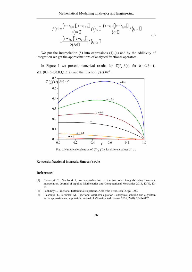
6. THE SIMPSON'S RULE FOR FRACTIONAL INTEGRAL OPERATORS
Tomasz Błaszczyk, Jarosław Siedlecki ........................................................ 25 7. FACIAL ASYMMETRY IN 3D FACE RECOGNITION
Janusz Bobulski ............................................................................................ 27 8. TRIDIAGONAL TOEPLITZ SYSTEMS: APPROACH BASED ON
LINEAR RECURRENCES VERSUS THOMAS METHOD Jolanta Borowska ......................................................................................... 33
9. THE EIGENFACES METHOD
Lena Caban ................................................................................................... 37 10. THE POLYNOMIAL INTERPOLATION BY THE KRONECKER
TENSOR PRODUCT Anita Ciekot ................................................................................................. 41
11. ANALYTICAL AND NUMERICAL SOLUTIONS OF DIFFERENT TYPES OF EQUATIONS USED FOR MODELING HEAT CONDUCTION UNDER LASER PULSE HEATING Mariusz Ciesielski ........................................................................................ 43

Mathematical Modelling in Physics and Engineering
6
12. UNCERTAINLY MEASUREMENT Jan Čapek, Martin Ibl ................................................................................... 45 13. MIXED-MODE LOAD TRANSFER IN THE FIBRE BUNDLE MODEL
OF NANOPILLAR ARRAYS Tomasz Derda ............................................................................................. 53
14. QUANTUM ENTANGLEMENT IN AVIAN NAVIGATION
Andrzej Drzewiński .................................................................................... 55 15. FUNCTIONS OF BOUNDED VARIATION AND THEIR PROPERTIES
Oliwia Fertacz, Agata Paluszewska ............................................................ 57 16. ALGORITHM OF REBUILDING A BOUNDARY OF DOMAIN
DURING CREATION OF AN OPTIMAL SHAPE Katarzyna Freus, Sebastian Freus ................................................................ 59
17. A DESIGN OF AN OPTIMAL SHAPE OF DOMAIN DESCRIBED
BY NURBS CURVES USING THE TOPOLOGICAL DERIVATIVE AND BOUNDARY ELEMENT METHOD
Katarzyna Freus, Sebastian Freus ................................................................ 61 18. THE USE OF THE IMAGE PROCESSING AND ANALYSIS METHODS
FOR OPTIMIZATION OF EQUATIONS OF MOTION FOR A QUADRUPED ROBOT Katarzyna Gospodarek ................................................................................ 63
19. HIGH PERFORMANCE NUMERICAL COMPUTING IN C++X11 Grzegorz Michalski, Andrzej Grosser ......................................................... 67 20. REPRESENTATIONS OF RIGHT HEREDITARY TENSOR ALGEBRAS
OF BIMODULES Nadiya Gubareni ........................................................................................ 69 21. MODELING OF MECHANICAL PHENOMENA IN THE PLATINUM-
CHROMIUM CORONARY STENTS Aneta Idziak-Jabłońska, Karolina Karczewska, Olga Kuberska .................. 71 22. AN INFLUENCE OF A ROD OF A VARIABLE CROSS-SECTION
AS A PART OF GEOMETRICALLY NONLINEAR COLUMN SUBJECTED TO THE SPECIFIC LOAD ON A VALUE OF BIFURCATION LOAD Anna Jurczyńska, Janusz Szmidla ................................................................ 73

Mathematical Modelling in Physics and Engineering
7
23. ON TWO-PARAMETER FELLER SEMIGROUP WITH NONLOCAL CONDITION FOR ONE-DIMENSIONAL DIFFUSION PROCESS
Bohdan Kopytko, Roman Shevchuk ............................................................ 75 24. MODELLING OF HEAT CONDUCTION IN A COMPOSITE SPHERE
USING FRACTIONAL CALCULUS Stanisław Kukla, Urszula Siedlecka ............................................................. 77
25. COMPARISON OF FREAK AND SURF ALGORITHMS FOR
RECOGNIZING KEY ELEMENTS FOR TIME-VARYING IMAGES Joanna Kulawik ........................................................................................... 79 26. DIRECT SAT-BASED CRYPTANALYSIS OF SOME SYMMETRIC
CIPHERS Mirosław Kurkowski ................................................................................... 81
27. ALGEBRAIC DEPENDENCE OF POLYNOMIAL MAPPINGS HAVING TWO ZEROS AT INFINITY Sylwia Lara - Dziembek .............................................................................. 83
28. EDGE ELECTRONIC PROPERTIES OF NANO-MATERIALS BASED ON
LARGE-SCALE FIRST-PRINCIPLE COMPUTATIONS Zhibing Li .................................................................................................... 85 29. SOLUTIONS OF SOME FUNCTIONAL EQUATIONS IN A CLASS OF
GENERALIZED HOLDER FUNCTIONS Maria Lupa .................................................................................................. 87
30. LINEAR RECURRENCES ALGORITHM FOR SOLVING TRIDIAGONAL
SYSTEMS WITH IMPLEMENTATION IN MAPLE Lena Łacińska ............................................................................................. 89
31. PROBLEM OF THE CONFLICTING AIMS IN THE PRODUCER-
CONSUMER MODEL Marek Ładyga ............................................................................................. 93
32. COMPARISON OF PARAMETERS CO-FERMENTATION PROCESS
OF MUNICIPAL SEWAGE SLUDGE WITH EXCESS SEWAGE SLUDGE FROM TREATED COKING WASTEWATER* Bartłomiej Macherzyński, Maria Włodarczyk-Makuła, Ewa Ładyga, Władysław Pękała ........................................................................................ 95
33. IMPROVE COMPUTATIONAL EFFICIENCY WITH THE LATEST PROGRAMMING LANGUAGES Grzegorz Michalski, Andrzej Grosser ......................................................... 99

Mathematical Modelling in Physics and Engineering
8
34. COALGEBRAS FOR MODELLING BEHAVIOUR
Valerie Novitzká, William Steingartner ..................................................... 101 35. THE JACOBIAN HAVING NON - GENERIC DEGREES
Edyta Pawlak .............................................................................................. 107 36. DIFFERANTIAL OPERATORS: THE ELLIPTICITY AND ITS
APPLICATIONS Antoni Pierzchalski .................................................................................... 109
37. THE DIRICHLET PROBLEM FOR THE TIME-FRACTIONAL HEAT
CONDUCTION EQUATION WITH HEAT ABSORPTION IN A MEDIUM WITH SPHERICAL CAVITY
Yuriy Povstenko, Joanna Klekot ................................................................ 111
38. NUMERICAL ANALYSIS OF SANDWICH PANELS SUBJECTED TO TORSION Zbigniew Pozorski ..................................................................................... 115
39. NUMERICAL ANALYSIS OF SANDWICH PANEL SUBJECTED TO MULTIPLE STATIC CONCENTRATED LOADS Zbigniew Pozorski, Łukasz Janik ............................................................... 117
40. ON A WEAK CONVERGENCE OF DENSITIES OF HOMOGENEOUS YOUNG MEASURES Piotr Puchała ............................................................................................... 119
41. FREE VIBRATION OF EULER-BERNOULLI BEAMS MADE OF AXIALLY FUNCTIONALLY GRADED MATERIALS Jowita Rychlewska ..................................................................................... 121
42. MULTI-LAYER NEURAL NETWORKS FOR SALES FORECASTING Magdalena Scherer ..................................................................................... 123
43. FEATURE EXTRACTION OF FOREARM-VEIN PATTERNS BASED ON REPEATED LINE TRACKING Dorota Smorawa, Mariusz Kubanek .......................................................... 127
44. AN INFLUENCE OF THE PARAMETERS OF LOADING HEADS ON THE LOADING CAPACITY OF A DAMAGED COLUMN SUBJECTED TO A SPECIFIC LOAD Krzysztof Sokół .......................................................................................... 133

Mathematical Modelling in Physics and Engineering
9
45. REMARKS ON THE IMPACT OF THE ADOPTED SCALE ON QUALITY OF PRIORITY ESTIMATION Tomasz Starczewski ................................................................................... 135
46. LEARNING TOOLS IN COURSE ON SEMANTICS OF PRORGAMMING LANGUAGES William Steingartner, Valerie Novitzká ..................................................... 137
47. EXTENDED THE TEMPERATURE ACTIVATION OF CARBON SATURATION STEEL PROCESS Katarzyna Szota ......................................................................................... 143
48. SAT-BASED VERIFICTION OF NSPKT PROTOCOL INCLUDING DELAYS IN THE NETWORK Sabina Szymoniak, Olga Siedlecka-Lamch, Mirosław Kurkowski ........... 145
49. THE PROBLEM OF FDM EXPLICIT SCHEME STABILITY Wioletta Tuzikiewicz ................................................................................. 147
50. EFFECT OF TORSIONAL RIGIDITY BETWEEN ELEMENTS ON FREE VIBRATIONS OF A TELESCOPIC HYDRAULIC CYLINDER SUBJECTED TO EULER’S LOAD Sebastian Uzny, Łukasz Kutrowski ........................................................... 151
51. ANALITICAL AND NUMERICAL SOLUTION OF THE HEAT CONDUCTION PROBLEM IN THE ROD Ewa Węgrzyn –Skrzypczak, Tomasz Skrzypczak ..................................... 153
52. INFLUENCE OF GROOVE WELD ON RESIDUAL STRESSES IN SINGLE-PASS BUTT WELDED JOINTS WITH THOROUGH PENETRATION Jerzy Winczek, Krzysztof Makles .............................................................. 157
53. QUEUEING SYSTEMS WITH LIMITED BUFFER SPACE AND LIMITED QUEUEING TIME Paweł Zając, Oleg Tikhonenko ................................................................... 159

Mathematical Modelling in Physics and Engineering
10

Mathematical Modelling in Physics and Engineering
11
MODELLING INTERFACIAL HEAT TRANSFER IN A 2-PHASE FLOW IN A PACKED BED
Dariusz Asendrych, Paweł Niegodajew
Institute of Thermal Machinery, Czestochowa University of Technology, Czestochowa, Poland [email protected]
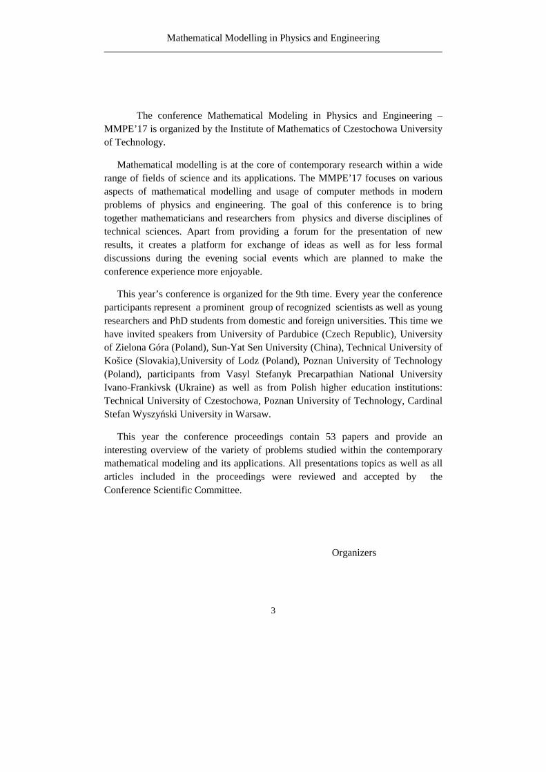
Packed beds are commonly used in various industrial processes. Drying, absorption or rectification can be mentioned as some typical examples. High efficiency of these multiphase (usually gas-liquid) processes is ensured by the enlarged contact area between working fluids provided by the packed bed filling. For typical working conditions, i.e. in the so-called trickling flow regime, liquid flows down driven by gravity, while gas freely moves up with no excessive flow resistance. Complex geometry of the packed bed filling makes the flow modelling challenging even for isothermal conditions. However, most of industrial processes indicate non-isothermal character, thus the heat transfer between working phases needs to be included in the governing equations. Unfortunately the existing source literature practically does not include any information about the interfacial heat transfer coefficients which are required to close the energy equation by the relevant source terms responsible for heat exchange between fluid phases.
Fig. 1. Schematic diagram of experimental facility
Mathematical Modelling in Physics and Engineering
12
The main objective of the present paper was to develop a correlation relating the interfacial heat transfer coefficient with the key flow/thermal parameters through the typical group numbers. The experiment was performed with the use of a small laboratory test rig schematically shown in Fig. 1. The distilled water and the ambient air were used as flowing media. The water was pumped from the container (5) and flowed through the filter (8), the flowmeter (18) and the distributor (21) supplying the column. Afterwards, it flowed through the packed bed (20) and it was collected in the tank (13) and reversed to the main container (5). Water flow was enforced by the pump (9) and controlled by operating valves (7) and (12). The column (19) was filled with 6 mm glass Raschig rings (20). The air flow was enforced by a vacuum pump (11). The air was sucked to the column at its bottom and flowed upward the packed bed. Then the air left the column through the outlet (23) and reached the cooler (17) where the water vapour was separated and collected in a tank (15), whereas the air passed through the gas flowmeter (16) and quited the test rig. Temperature of the water in the main container was kept constant with the use of a temperature controller (3) connected to a thermocouple (4) and a heater (6). Temperatures of working media were measured upstream and downstream the packing section with the thermocouples (25) and (30) for gas while (24) and (31) for liquid. The signals from all sensors were sent through the AD converter (2) to the PC (1) for data acquisition and postprocessing. Additionally the air humidity was measured with the sensors (29) and (26). More information about the experiment and the measurement procedure can be found in [1].
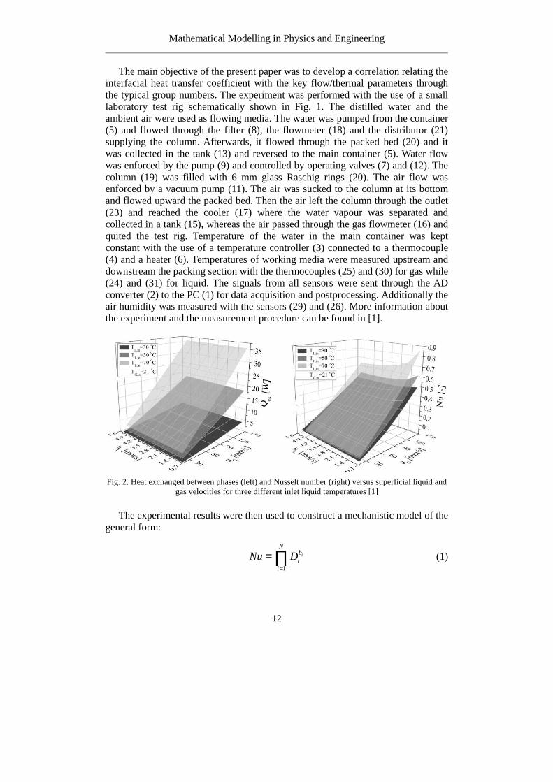
Fig. 2. Heat exchanged between phases (left) and Nusselt number (right) versus superficial liquid and
gas velocities for three different inlet liquid temperatures [1]
The experimental results were then used to construct a mechanistic model of the general form:
1
i
Nbi
i
Nu D=
= ∏ (1)

Mathematical Modelling in Physics and Engineering
13
where Di stands for a set of group numbers and bi (i=1, …, N) is the matrix corresponding to their exponents to be found by fitting experimental data. According to [3] the Reynolds, Galileo, Prandtl, Eötvös and Grashof numbers are regarded as the most relevant group numbers to describe the heat transfer processes in a 2-phase flow system. In this way viscous, inertial, gravity, surface tension and buoyancy effects can be taken into account. After detailed and multi-step regression analysis the correlation of the following form was proposed:
1.169 0.8399 0.7176ReG GNu Ga Eo−= ⋅ ⋅ ɺɺ (2)
characterised by the correlation coefficient R = 0.992 indicating very good correspondence between experimental and modelled Nu values. Index "G" in the above formula stands for the gas phase.
The regression analysis is summarised in graphical form in Fig. 3 presenting the parity plot of the modelled Nusselt number (formula (2)) against the experimental data. In order to make it easier to interpret the results the solid lines corresponding to ±10% errors are plotted in the graph. As can be seen the proposed correlation fits the measured data with very high accuracy characterised by the correlation coefficient equal to 0.992. Very few data points lie outside the ±10% limit and they correspond to the lowest liquid load range where the increased measurement uncertainty may be expected.
Fig. 3. Parity plot for experimental and modelled Nusselt number values [2]
It should be remarked that the correlation was developed for the limited range of gas and liquid loads and for particular type and size of catalyst elements. Thus, there is a need of further research work, including much wider gas and liquid loads as well as different random packing element types and sizes, to provide better

Mathematical Modelling in Physics and Engineering
14
understanding of the heat transfer processes in complex geometrical constraints. The wetting efficiency of the packed bed seems to be one of the most important factors governing the interfacial heat transfer. The existing correlations need further development to provide better precision and thus to allow accurate estimation of the interface contact area. The correlation developed in the present paper is planned to be used in the forthcoming numerical research devoted to the 2-phase gas-liquid flow in a porous media. It will be incorporated to an existing CFD (computational fluid dynamics) model allowing for adequate modelling of such complex physio-chemical processes as carbon dioxide chemical absorption in packed beds.
Keywords: porous media, 2-phase flows, interfacial heat transfer, regression analysis
References
[1] Niegodajew P., Asendrych D., An Interfacial Heat Transfer In a Countercurrent Gas-Liquid Flow in a Trickle Bed Reactor, Int. J. of Heat & Mass Transfer, 108A, 2017, 703-711.
[2] Niegodajew P., Asendrych D.: Experimental Study of Gas-Liquid Heat Transfer in a 2-phase Flow in a Packed Bed, Journal of Physics: Conference Series 745, 2016, 032139.
[3] Ghajar A.J., Non-boiling Heat Transfer in Gas-Liquid Flow in Pipes: A Tutorial, J. Brazilian Soc. Mech. Sci. Eng. 27, 2005, 46-73.

Mathematical Modelling in Physics and Engineering
15
MODELLING OF QUASI-COHERENT DISPLACEMENT IN CHAIN-LIKE BODIES’ MOVEMENT
Kamila Bartłomiejczyk
Institute of Mathematics, Czestochowa University of Technology, Czestochowa, Poland
The article concerns the extension of the sequential algorithm which has been previously described e.g. in [1-3]. This algorithm can be used for simulation of the chain-like bodies’ movement. One of the most widely studied phenomenon which is associated with the chain motion is the chain translocation through the pore in membrane (see e.g. [4-11]). The translocation process plays a crucial role in many processes. It is applied inter alia in DNA and RNA sequencing techniques [10-14], controlled drug delivery process [15-17] or gene therapy [18, 19].
Many different algorithms are used in literature for the analysis of the chain-like structures movement (see e.g. [4-9, 20, 21]). Therefore, it seems to be reasonable to create an efficient algorithm which can reflect the chain behaviour as good as it possible. In this paper the following extensions of the sequential algorithm for the simulation of the chain-like bodies’ motion are described: compression propagation mechanism and movement-direction preference mechanism. The former is the extension of the tension propagation which has been described in [2]. It can be said that the compression propagation mechanism allows for ‘pushing’ of the segment which is moving by the previously moved segment. In [2] only ‘pulling’ of moving segment is possible. Implementation of the movement-direction preference mechanism causes that the direction of the moving segment step depends on the position of the segment which has been moved previously. In other words, the moving segment is pulled (or pushed) in the direction of the previously moved segment. In the article the implementation of these mechanisms is described, the parameters associated with them are defined and the influence of these parameters on the translocation time is analysed.
Keywords: algorithm, chain-like structure, compression propagation, movement-direction preference, translocation time
References
[1] Grzybowski A.Z., Domanski Z., A sequential algorithm for modeling random movements of chain-like structures, Sci. Res. Inst. Math. 2011, 10(1), 5-10.
[2] Grzybowski A. Z., Domański Z., A sequential algorithm with built in tension-propagation mechanism for modeling the chain-like bodies dynamics, arXiv:1312.4206 [cond-mat.soft].
Mathematical Modelling in Physics and Engineering
16
[3] Grzybowski A.Z., Domański Z., Bartłomiejczyk K., Algorithmization and simulation of the chain-like structures' dynamics-interrelations between movement characteristics, Acta Eletrotechnica et Informatica, 2013, Vol 13 (4).
[4] van Leeuwen J.M., Drzewiński A., Stochastic lattice models for the dynamics of linear polymers, arXiv:1004.2370 [cond-mat.stat-mech].
[5] Żurek S., Kośmider M., Drzewiński A., J. M. J. van Leeuwen, Translocation of polymers in a lattice model, The European Phys. J. E: Soft Matter and Biological Physics. 2012, 35: 47.
[6] Luo K., Huopaniemi I., Ala-Nissila T., Ying S.C., Polymer translocation through a nanopore under an applied external field, The Journal of chemical physics, 2006, 124 (11), 114704.
[7] Luo K., Ala-Nissila T., Ying S.C., Polymer translocation through a nanopore: A two-dimensional Monte Carlo Study, The Journal of chemical physics, 2006, 124 (3), 034714.
[8] Chuang J., Kantor Y., Kardar M., Anomalous dynamics of translocation, Physical Review E, 2001, 65, 011802.
[9] Gauthier M.G. Slater G.W., A Monte Carlo algorithm to study polymer translocation through nanopores. I. Theory and numerical approach, The Journal of Chemical Physics, 2008, 128, 065103.
[10] Meller A., Nivon L., Branton D., Voltage-Driven DNA Translocation through a Nanopore, Physical Review Letters, 2001, 86, 3435.
[11] Muthukumar M., Mechanism of DNA transport through pores, Annual Reviews Biophysics and Biomolecular Structure, 2007, 36, p. 435-50.
[12] Feng Y., Zhang Y., Ying C., Wang D., Du C., Nanopore-based Fourth-generation DNA Sequencing Technology, Genomic Proteomics Bioinformatics, 2015, 13, p. 4-16.
[13] Wanunu M., Nanopores: A journey toward DNA sequencing, Physics of Life Reviews, 2012, 9 (2), p. 125-158.
[14] Haque F., Li J., Wu H., Liang X., Guo P., Solid-state and biological nanopore for Real-time sensing of single chemical and sequencing of DNA, Nano Today, 2013, 8, p 56-74.
[15] Tsutsui J.M.., Xie F., Porter R.T., The use of microbubbles to target drug delivery, Cardiovascular Ultrasound, 2004, 2:23-30.
[16] Tseng YL., Liu JJ., Hong RL, Translocation of Liposomes into Cancer Cells by Cell-Penetrating Peptides Penetratin and Tat: A Kinetic and Efficacy Study, Molecular Parmacology, 2002, 62:864-872.
[17] Merkle H.P., Drug delivery’s quest for polymers: Where are the frontiers?, European Journal of Pharmaceutics and Biopharmaceutics, 2015, 97, p. 293-303.
[18] Jeong J.H., Kim S.W., Park T.G., Molecular design of functional polymers for gene therapy, Progress in Polymer Science, 2007, 32, p. 1239-1274.
[19] Wong S.Y., Pelet J.M., Putnam D., Polymer systems for gene delivery – Past, present and Future, Progress in Polymer Science, 2007, 32, p. 799-837.
[20] Drzewiński A., van Leeuwen J.M., Crossover from Reptation to Rouse dynamics in the Extended Rubinstein-Duke Model, Phys. Rev. E, 2007, 77, 03 1802.
[21] D’Adamo G., Pelissetto A., Pierleoni C., Polymers as compressible soft spheres, arXiv: 1205.5654v1, [cons-matt.soft].

Mathematical Modelling in Physics and Engineering
17
THE PROOF OF REMARK ON THE JACOBIAN CONJECTURE
Grzegorz Biernat
Institute of Mathematics, Czestochowa University of Technology, Czestochowa, Poland
Let ( ) 2 2, :f h →ℂ ℂ be the polynomial mapping having two zeros at infinity.
Remark. Let
( ) 2 1 2 2 2 3 1...p
p p pf XY f f f f− − −= + + + + + (1)
( ) 2 1 2 2 2 3 1...q
q q qh XY h h h h− − −= + + + + + (2)
where 1p q≥ ≥ and fi, hj be the complex forms of variables X, Y of degrees i, j respectively. If ( ) ( )1 1Jac , Jac ,f h const f h= = then
2 1
1 1
q
k kX Y h−
− − and
1
1 12 11 2 11 2 11
1 1 1...
p p
pq q qf X Y h A X Y h A X Y hq q q
−
−− − −
= + + + + + +
(3)
1
1 12 11 2 11 2 11
1 1 1...
q q
qq q qh X Y h B X Y h B X Y hq q q
−
−− − −
= + + + + + +
(4)
for some constants 1 1 1 1,..., , ,...,p qA A B B− − . The form 2 11qh − is defined by the
formula 2 1
1 12 11q
q qqh X Y h
−
− −−= .
Sketch of the proof.
For q = 1 the remark is true. Let 2p ≥ . We assume that the formula (3) and (4) are true for exponents q = 1, ..., p – 1. We will prove that for q = p the formulas are also true. Let's save again the formulas (1) and (2) for q = p
( ) 1) 2) 3)
2 1 2 2 2 3 1...p
p p pf XY f f f f− − −= + + + + + (5)
and

Mathematical Modelling in Physics and Engineering
18
( ) 1) 2) 3)
2 1 2 2 2 3 1...p
p p ph XY h h h h− − −= + + + + + (6)
Consecutively we have
2 1 2 1p ph f− −= (7)
( ) 1
2 2 1 2 2
p
p ph A XY f−
− −+ = (8)
We obtain
( ) ( ) 1
2 1 2 2 1 2 3 1...p p
p p pf XY h h A XY f f−
− − −= + + + + + + (9)
and
( ) 2 1 2 2 2 3 1...p
p p ph XY h h h h− − −= + + + + + (10)
Let 1 0A ≠ . We assume
( ) ( ) ( ) ( )
( )
1
2 3 2 3 1 11 1 1
1
2 3 1
1 1 1...
....
p
p p
p
p
f f h XY f h f hA A A
XY f f
−− −
−−
= − = + − + + − =
= + + +
ɶ
ɶ ɶ
(11)
Then
( ) ( )1
1Jac , Jac ,h f f h const
A= − =ɶ (12)
Now we convert f to h and h for fɶ and apply the induction assumption for
exponent p – 1,. Therefore ( ) 2
2 3
p
pXY f−
−ɶ , which allows to determine the form
2 3 1pf −ɶ . We have
1
1 12 3 1 2 3 1 2 3 1
1 1 1...
1 1 1
p p
pp p ph XY f B XY f B XY fp p p
−
−− − −
= + + + + + + − − −
ɶ ɶ ɶ
(13) and
1 1
1 22 3 1 2 3 1 2 3 1
1 1 1...
1 1 1
p p
pp p pf XY f A XY f A XY fp p p
− −
−− − −
= + + + + + + − − −
ɶ ɶ ɶ ɶɶ ɶ
(14)

Mathematical Modelling in Physics and Engineering
19
for some constants 1B , …, 1pB − ; 1Aɶ , …, 2pA −ɶ . Moreover
( ) 1
2 1 2 3 11p
p p
ph XY f
p
−− −=
−ɶ (15)
so ( ) 1
2 1
p
pXY h−
− . From the formula (15) we obtain
2 1 1 2 3 1
1 1
1p ph fp p− −=
−ɶ (16)
So
1 2
1 22 1 1 2 1 1 2 1 1
1 1 1...
p p
pp p pf XY h A XY h A XY hp p p
− −
−− − −
= + + + + + +
ɶ ɶ ɶ (17)
and
1
1 12 1 1 2 1 1 2 1 1
1 1 1...
p p
pp p ph XY h B XY h B XY hp p p
−
−− − −
= + + + + + +
(18)
Therefore
1
1 2
1 1 22 1 1 2 1 1 2 1 1
1 2
1 22 1 1 2 1 1 2 1 1
1 2 1 1
1 1 1...
1 1 1...
1
p p
pp p p
p p p
p p p
p p
f h A f
h A XY h A XY h A XY hp p p
XY h A XY h A XY hp p p
A XY hp
− −
−− − −
− −
− − −
− −
= + =
= + + + + + + +
= + + + + + + +
+ +
ɶ
ɶ ɶ
(19)
If A1= 0 we have analogously
( ) 2
2 4 2 2 4
p
p ph A XY f−
− −+ = (20)
and with the constant A2 we proceed in the same way as the constant A1.
Keywords: Jacobian, zeros at infinity, Jacobian Conjecture

Mathematical Modelling in Physics and Engineering
20
References
[1] Abhyankar S.S., Expansion techniques in algebraic geometry, Tata Inst. Fundamental Research, Bombay, 1977.
[2] Charzyński Z., Chądzyński J., Skibinski P., A contribution to Keller’s Jacobian Conjecture, Lecture Notes In Math. 1165, Springer-Verlag, Berlin Heidelberg N. York, 36-51, 1985.
[3] Bass H., Connell E.H., Wright D., The Jacobian conjecture: reduction of degree and formal expansion of the inverse, American Mathematical Society. Bulletin. New Series 7 (2): 287–330, 1982.
.

Mathematical Modelling in Physics and Engineering
21
A REVIEW OF NUMERICAL METHODS FOR FRACTIONAL ORDINARY DIFFERENTIAL EQUATIONS
Marek Błasik
Institute of Mathematics, Czestochowa University of Technology, Czestochowa, Poland
In recent years there has been an increase in the number of publications devoted to differential equations of fractional order, which are widely applied in modeling many problems in: physics, control theory, bioengineering and mechanics [1,2,3].
In many cases, obtaining an analytical solution for fractional differential equations is very difficult, or even impossible, then we apply numerical methods.
Consider a one-term fractional differential equation including the left-sided Caputo derivative:
( ]1,0)),(,()(0 ∈=+ αψα tfttfDC , (1)
with initial condition
0)0( ff = . (2)
The starting point for the all numerical methods discussed in the paper is transformation of the initial value problem (1-2) into an equivalent integral equation:
).0())(,()( 0 ftftItf += +ψα (3)
We compare numerical results obtained by Euler method [4] and two variants of Adams-Bashforth-Moulton (A-B-M) method [4,5]. In Euler method we apply rectangle rule to calculate integral in formula (3). First variant of (A-B-M) method requires trapezoidal rule to calculate corrector. The second one requires two methods to determine the corrector: Simpson's rule or trapezoidal rule depending on an odd or even number of nodes in the integration interval.

Mathematical Modelling in Physics and Engineering
22
Fig. 1. Exact and numerical solutions of equation (1) where )())(,( tftft =ψ , 1)0( =f ,
75.0=α .
Fig. 2. The absolute error generated by numerical methods.
Keywords: fractional calculus, fractional differential equations, fractional integral equations, numerical methods
References
[1] Magin R.L., Fractional Calculus in Bioengineering, Begell House Publisher, Redding, 2006. [2] Kosztołowicz T. Zastosowanie Równań Różniczkowych z Pochodnymi Ułamkowymi do Opisu
Subdyfuzji. Wydawnictwo Uniwersytetu Humanistyczno-Przyrodniczego Jana Kochanowskiego, Kielce, 2008.
[3] Ostalczyk P. Zarys Rachunku Różniczkowo-Całkowego Ułamkowego Rzędu, Wydawnictwo Politechniki Łódzkiej, Łódź, 2008.
[4] Diethelm K. The Analysis of Fractional Differential Equations. Springer-Verlag, Berlin, 2010. [5] Błasik M. A new variant of Adams-Bashforth-Moulton method to solve sequential fractional
ordinary differential equation. 21th International Conference on Methods and Models in Automation and Robotics (MMAR), Międzyzdroje, Poland, 2016, 854-858.
Mathematical Modelling in Physics and Engineering
23
APPROXIMATION OF FRACTIONAL INTEGRALS BASED ON B-SPLINE INTERPOLATION
Tomasz Błaszczyk, Jarosław Siedlecki
Institute of Mathematics, Czestochowa University of Technology, Czestochowa, Poland
[email protected], [email protected]
In this paper, we propose a new approach to the numerical evaluation of the fractional integral operators. The presented methodology is performed by utilizing the well-known B-spline interpolation [1].
We introduce definitions of fractional integral operators. The left and right fractional Riemann-Liouville integrals of order Rα +∈ are defined respectively
(see [2])
( ) ( )( )
( )1
1: d , for
x
aa
fI f x
xx a+
α−α
τ= τ >
Γ α − τ∫ (1)
( ) ( )( )
( )1
1: d , for
bx
b fI f x b
xx−
α−α
τ= τ <
Γ α τ −∫ (2)
where Γ denotes the Gamma function. The interval [ , ]a b is divided into N sub-
intervals 1[ , ]i ix x+ with a constant step ( ) /h b a N= − . Next, we replace the function f by the following expression
( ) ( )1
1
N
j jj
S K xx B+
=−
= ∑ (3)
where the B-splines are defined in the following way
( )
( )( ) ( ) ( )( ) ( ) ( )
( )
3
2 2 1
2 33 21 1 1 1
2 33 23
1 1 1 1
3
2 1 2
3 3 31
3 3 3
othe is0 rw e
j j j
j j j j j
jj j j j j
j j j
x x x x x
h h x x h x x x x x x x
B h h x x h x x x x x x xh
x x x x
x
x
− − −
− − − −
+ + + +
+ + +
− ≤ < + − + − − − ≤ <= + − + − − − ≤ < − ≤ <
(5)
and coefficients 1 0 1, , , NK K K− +… are obtained by solving the matrix equation

Mathematical Modelling in Physics and Engineering
24
( )( )( )
( )( )( )
1 0
0 0
1
1
1
3 30 0 0 0 '
1 4 1 0 0 0
0 1 4 1 0 0
0 0 1 4 1 0
0 0 0 1 4 1
'3 30 0 0 0
N
N N
N N
K f xh hK f x
f x
f x
K f x
K f x
h h
−
−
+
− =
−
⋯
⋯
⋯
⋮ ⋮⋱
⋯
⋯
⋯
(4)
In Figure 1 we present numerical evaluation of ( )3
11I x−
α − for 5N =
Fig. 1. Numerical (points) and analytical (lines) results for different values of α .
Keywords: fractional integrals, B-spline interpolation
References
[1] Majchrzak E., Mochnacki B., Metody numeryczne. Podstawy teoretyczne, aspekty praktyczne i algorytmy, Wyd. Pol. Śl., Wydanie IV rozszerzone, Gliwice 2004.
[2] Podlubny I., Fractional Differential Equations, Academic Press, San Diego 1999.

Mathematical Modelling in Physics and Engineering
25
THE SIMPSON'S RULE FOR FRACTIONAL INTEGRAL OPERATORS
Tomasz Błaszczyk, Jarosław Siedlecki
Institute of Mathematics, Czestochowa University of Technology, Czestochowa, Poland
[email protected], [email protected]
In this paper, we propose an approach based on quadratic interpolation to the numerical evaluation of the composition of the left and right Riemann-Liouville integrals. The presented methodology is a fractional equivalent to the classical Simpson's rule [1]. We calculate errors and determine the experimental rate of convergence for the described approach.
First, we will introduce definitions of fractional integral operators. The left and right fractional Riemann-Liouville integrals of order Rα +∈ are defined respectively (see [2])
( ) ( )( )
( )1
1: d , for
t
aa
fI f t t a
t+
α−α
τ= τ >
Γ α − τ∫ (1)
( ) ( )( )
( )1
1: d , for
b
bt
fI f t t b
t−
α−α
τ= τ <
Γ α τ −∫ (2)
where Γ denotes the Gamma function. Fractional integral operators, which are a composition of the left and right fractional Riemann-Liouville integrals, look as follows (see [3])
( ) ( ) [ ],1
,: , for ,
a b a bf t I I f t t a b+ − + −
α α α= ∈I (3)
( ) ( ) [ ],1
,: , for ,
b a b af t I I f t t a b− + − +
α α α= ∈I (4)
The interval [ , ]a b is divided into N (even) sub-intervals 1[ , ]i it t + , for
0,1,., 1i N= − with a constant step ( ) /t b a N∆ = − by using nodes it a i t= + ∆ . Next, we replace function f by the quadratic polynomial, which takes the same
values as f at the end points 2 jt and 2 2jt + , and the midpoint 2 1jt +
Mathematical Modelling in Physics and Engineering
26
( ) ( )( )( )
( ) ( )( )( )
( )
( )( )( )
( )
2 1 2 2 2 2 2
2 2 12 2
2 2 1
2 22
2
2
j j j j
j j
j j
j
t t t tf f t f t
t t
t tf t
t
+ + ++
++
τ − τ − τ − τ −τ ≈ −
∆ ∆
τ − τ −+
∆
(5)
We put the interpolation (5) into expressions (1)-(4) and by the additivity of integration we get the approximations of analysed fractional operators.
In Figure 1 we present numerical results for ,1
,( )
a bf tα
+ −I for 0, 1a b= = ,
0.4,0.6,0.8,1,1.5,2α ∈ and the function ( )f t tα= .
Fig. 1. Numerical evaluation of ,1
,10( )f tα
+ −I for different values of α .
Keywords: fractional integrals, Simpson's rule
References
[1] Blaszczyk T., Siedlecki J., An approximation of the fractional integrals using quadratic interpolation, Journal of Applied Mathematics and Computational Mechanics 2014, 13(4), 13-18.
[2] Podlubny I., Fractional Differential Equations, Academic Press, San Diego 1999. [3] Blaszczyk T., Ciesielski M., Fractional oscillator equation - analytical solution and algorithm
for its approximate computation, Journal of Vibration and Control 2016, 22(8), 2045-2052.

Mathematical Modelling in Physics and Engineering
27
FACIAL ASYMMETRY IN 3D FACE RECOGNITION
Janusz Bobulski
Institute of Information and Computer Science, Czestochowa University of Technology, Czestochowa, Poland [email protected]
Introduction
Biometrics systems use individual and unique biological features of person for user identification. The most popular features are: fingerprint, iris, voice, palm print, face image et al. Most of them are not accepted by users, because they feel under surveillance or as criminals. Others, in turn, are characterized by problems with the acquisition of biometric pattern and require closeness to the reader. Among the biometric methods popular technique is to identify people on the basis of the face image, the advantage is the ease of obtaining a biometric pattern. Low prices of cameras have caused their commonness and they are everywhere. Moreover, the quality of the images captured from modern cameras are so good that they may be used to retrieve biometric patterns, and then for identification. The advantage of the identification with the face image is the ease acquiring pattern and a high acceptance level of this method by users. There are many works on 2D face recognition [1], and made great progress in this field. Among these works there are also techniques that use the asymmetry of the face, and the efficiency of this technique is confirmed in articles [2-5]. With the development of 3D technology appeared methods of 3D face recognition. In last years, some of the new face recognition strategies tend to overcome face recognition problem from a 3D perspective. The 3D data points proper to the surface of the face give us other kind of information for recognition, and solve the problem of pose and lighting variations in case of 2D data. However, 3D images have their own problems, e.g. normalization, devices for acquiring faces, time and cost of faces getting [6]. In the literature, we may find a lot of useful reviews of 3D face recognition problem such as [7].
Many works are dedicated to the 3D face recognition problem. There is the method presented by Riccio et al. [8] among them, that uses predefined key points. These points are used to indicate the several geometric invariants on the basis of which is made identification. Other method, Rama et al. present in article [9]. They propose Partial Principle Component Analysis (P2CA) for feature extraction and dimensionality reduction by projection 3D data into cylindrical coordinate. In [10], researchers use the iterative closest point (ICP) to adjust the 3D surface points of a face and then realize the recognition based on the minimum distance between the two faces . These methods have high recognition rate, but their main problem is speed and computational complexity.
Mathematical Modelling in Physics and Engineering
28
Using of 3D images for the identification was in a field of the interest of many researchers which developed a few methods offering good results [11]. However, there are few techniques exploiting the 3D asymmetry amongst these methods. The reason for this is, among others, the problem of obtaining 3D images. The cost 3D camera is still higher than traditional camera and therefore their popularity and prevalence is lower. The second major problem in the processing of 3D images is their quality. Imperfection devices for image acquisition cause errors in the measurements and data discontinuity, that is a significant problem in the further processing of the data. At the present moment, however, we need to use the data in the quality of such is, and try to eliminate the disadvantages of these data and develop more effective methods of asymmetry measurement and face recognition based on asymmetry.
Few papers in the literature are dedicated to the 3D asymmetry face recognition task so far. Huang et al. [12] propose method based on Local Binary Pattern (LBP). Their approach splits the face recognition task into two steps: (1) a matching step respectively processed in 2D/2D; (2) 3D/2D a fusion step combining two matching scores. Canonical Correlation Analysis (CCA) is applied in method propose by Yang et al. [13]. They apply CCA to learn the mapping between the 2D face image and 3D face data, and only 3D data is used for enrolment and recognition. This article presents face recognition method based on 3D face asymmetry. We propose fast algorithm for rough extraction face asymmetry that is used to 3D face recognition with hidden Markov models (HMM) [14].
PROPOSED METHOD
The pre-processing procedure of the system consists of the following steps: selection of face area, scaling image, rotation. The main area of the face selected and rejected areas that contain little useful information on the outskirts of face. The selection of face area made based on key points, and the coordinates of these points are obtained from database. Based on inner corners of the eyes, the face image is scaled so that the distance between them was equal to 120 pixels. Next, the angle of rotation is calculated from the mentioned coordinates, and face image is rotated by an angle alpha. This operation is aimed at establishing the identical position for all faces.
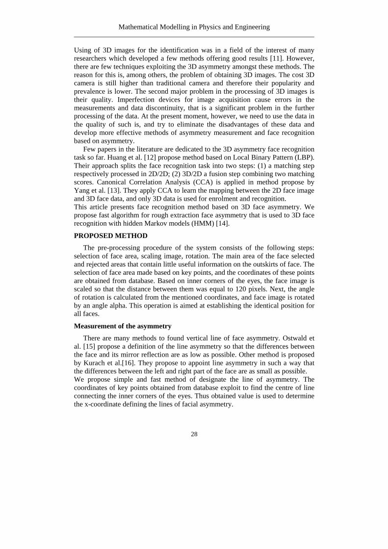
Measurement of the asymmetry
There are many methods to found vertical line of face asymmetry. Ostwald et al. [15] propose a definition of the line asymmetry so that the differences between the face and its mirror reflection are as low as possible. Other method is proposed by Kurach et al.[16]. They propose to appoint line asymmetry in such a way that the differences between the left and right part of the face are as small as possible. We propose simple and fast method of designate the line of asymmetry. The coordinates of key points obtained from database exploit to find the centre of line connecting the inner corners of the eyes. Thus obtained value is used to determine the x-coordinate defining the lines of facial asymmetry.

Mathematical Modelling in Physics and Engineering
29
In this way we are dividing the face into the right and left part. Through the mirror vertically they are rising from these parts right face (RF) and left face (LF). From z-coordinate of these two elements and the normal face (NF) the measurement of the asymmetry is being made. In this way, the three metrics are formed that are differences between the RF, LF and NF (eq.1-3).
LN= |LF - NF| (1)
RN= |RF - NF| (2)
LR= |LF - RF| (3)
Fig. 1. Results of the measurement of the face asymmetry
Mathematical Modelling in Physics and Engineering
30
Recognition system
We have two basic tasks in face recognition application: learning and testing. In case of HMM [17], first task is made with Baum-Welch algorithm, that is based on the forward-backward algorithm. Second task may be made in some ways, but we chose forward algorithm.\\ Forward Algorithm [18]: Define forward variable ( )tjα as:
( ) ( ) ( )rtj
N
jijij obatt
−= ∑
−
=
1
2
1αα (4)
Backward Algorithm [18]: Define backward variable ( )tiβ as:
( ) ( ) ( )∑−
=+ +=
1
21 1
N
jj
rtjiji tobat ββ (5)
Baum-Welch Algorithm [18]:
( ) ( ) ( ) ( )( )
( ) ( ) ( )( ) ( ) ( )
1 1 1 1
1 11 1
,|
ij j t t ij j t t
N N
t ij j t ti j
i a b o j i a b o ji j
P Oi a b o j
α β α βξ
λ α β
+ + + +
+ += =
= =∑∑
(6)
Experiments
In experiments we used the image database UMB-DB. The University of Milano Bicocca 3D face database is a collection of multimodal (3D + 2D colour images) facial acquisitions. The database is available to universities and research centres interested in face detection or face recognition. They recorded 1473 images of 143 subjects (98 male, 45 female). The images show the faces in variable condition, lighting, rotation and size [19]. We chose three datasets, each consist of 50 persons in order to verify the method, and for each individual chose two images for learning and two for testing. The HMM implemented with parameters N = 10, O = 20. Table 1 presents the results of experiments.

Mathematical Modelling in Physics and Engineering
31
Table 1. Results of experiments
Type of asymetry No. of test set Recognition rate [%] LN 1 58 LN 2 62 LN 3 60
Average 60 RN 1 58 RN 2 60 RN 3 62
Average 60 LR 1 68 LR 2 70 LR 3 72
Average 70
Table 2. Comparison to other methods
Method Recognition rate [%] LBP 82 CCA 68 Our 70
Conclusion
This paper presented conception of fast and rough method for determines 3D face asymmetry. Presented method allows for faster 3D face processing and recognition because they do not use complex calculation for features extraction. The obtained results are satisfactory in comparison to other method and proposed method may be the alternative solution to the others. Experiments confirmed the validity of the concept of 3D face asymmetry, and it is a faster method in comparison to another. The research results indicate that face recognition with 3D face asymmetry may be used in biometrics systems.
Keywords: face 3D, facial asymmetry, face recognition
References
[1] Zhao W., Chellappa R., Phillips P., Rosenfeld A. (2003) Face recognition: A literature survey, ACM Computing Surveys 35 (4): 399–458.
[2] Mitra S, Lazar NA, Liu Y. (2007) Understanding the Role of Facial Asymmetry in Human Face Identification, Journal Statistics and Computing 17 (1): 57–70.
[3] Kubanek M, Rydzek S. (2008) A Hybrid Method of User Identification with Use Independent Speech and Facial Asymmetry, Lecture Notes in Artificial Intelligence, 5097: 818–827.
[4] Zhang G, Wang Y. (2009) Asymmetry Based Quality Assessment of Face Images. Lecture Notes in Computer Science, 5876, 499–508.
[5] Kompanets L. (2004) Biometrics of Asymmetrical Face, Biometric Authentication. Lecture Notes in Computer Science 2004, 3072: 67–73.
Mathematical Modelling in Physics and Engineering
32
[6] Mahoor M., Abdel-Mottaleb M. (2009) Face recognition based on 3d ridge images obtained from range data, Pattern Recognition 42 (3): 445–451.
[7] Abate A., Nappi M., Riccio D., Sabatino G. (2007) 2d and 3d face recognition: A survey, Pattern Recognition Letters 28(14): 1885–1906.
[8] Riccio D., Dugelay J.L. (2005) Asymmetric 3D/2D Processing: A Novel Approach for Face Recognition, Image Analysis and Processing ICIAP 2005, Vol. 3617, Lecture Notes in Computer Science: 986–993.
[9] Rama A., Tarres F., Onofrio D., Tubaro S. (2006) Mixed 2D-3D information for pose estimation and face recognition, ICASSP, II: 361–368.
[10] Beumier C., Acheroy M. (2000) Automatic 3D face authentication, Image and Vision Computing, 18(4): 315 – 321.
[11] K. Bowyer, K. Chang, P. Flynn (2006) A survey of approaches and challenges in 3d and multimodal 3d+2d face recognition, Comput. Vision Image Understanding 101: 1–15.
[12] Huang D., Ardabilian M., Wang Y., Chen L. (2009) Asymmetric 3d/2d face recognition based on lbp facial representation and canonical correlation analysis, International Conference on Image Processing: 3325–3328.
[13] Yang W., Yi D., Lei Z., Sang J., Li S. (2008) 2D-3D face matching using CCA, 8th IEEE International Conference on Automatic Face & Gesture Recognition, 2008. FG ’08: 1–6.
[14] Bobulski J. (2016) 2DHMM-Based Face Recognition Method, Image Processing and Communications Challenges 7, Advances in Intelligent Systems and Computing, Vol. 389: 11–18.
[15] Ostwald J., Berssenbrggea P., Dirksena D., Runtea Ch., Wermkerb K., Kleinheinzc J., Jungc S. (2015) Measured symmetry of facial 3D shape and perceived facial symmetry and attractiveness before and after orthognathic surgery, Journal of Cranio-Maxillofacial Surgery, Vol. 43 (4): 521–527
[16] Kurach D., Rutkowska D. (2012) Influence of Facial Asymmetry on Human Recognition, Artificial Intelligence and Soft Computing: 11th International Conference, ICAISC 2012, Zakopane, Poland, April 29-May 3, 2012, Proceedings, Part II, Springer Berlin Heidelberg: 276–283.
[17] Samaria F., Young S. (1994) HMM-based Architecture for Face Identification, Image and Vision Computing, Vol. 12 No 8 October: 537–583.
[18] Kanungo T. (1999) Hidden Markov Model Tutorial, http://www.kanungo.com/software/hmmtut.pdf
[19] Colombo A., Cusano C., Schettini R. (2011) UMB-DB: A Database of Partially Occluded 3D Faces, Proc. ICCV 2011 Workshops: 2113–2119.

Mathematical Modelling in Physics and Engineering
33
TRIDIAGONAL TOEPLITZ SYSTEMS: APPROACH BASED ON LINEAR RECURRENCES VERSUS THOMAS METHOD
Jolanta Borowska
Institute of Mathematics, Czestochowa University of Technology, Czestochowa, Poland
The subject of considerations are linear systems of algebraic equations of a tridiagonal Toeplitz type. The subsequent analysis will be restricted to the systems which have the unique solutions. We are to compare the two methods: approach based on linear recurrences and Thomas algorithm. First of them was proposed for the general tridiagonal system in [1] where the corresponding recurrence equations are shown. Thomas algorithm is well known in literature, [2,3]. A linear algebraic tridiagonal Toeplitz system for n unknowns has the form
1 2 1
1 1
1
, 2,..., 1k k k k
n n n
ax cx d
bx ax cx d k n
bx ax d− +
−
+ = + + = = − + =
(1)
We start with approach based on linear recurrences which is given in [1]. In order to apply this method it is convenient to represent system (1) by the corresponding matrix equation
dxA =⋅n (2)
where
=
ab
cab
cab
cab
ca
n
00
0
0
00
……
⋱⋮
⋱⋱⋱⋱⋮
⋮⋱
⋮⋱
……
A ,
=
−
n
n
x
x
x
x
x
1
3
2
1
⋮x ,
=
−
n
n
d
d
d
d
d
1
3
2
1
⋮d
Let us denote by nW the determinant of the matrix nA . As we consider the system
which has the unique solution, we must to assume that 0≠nW . It can be pointed out that first of the presented methods doesn’t impose any additional conditions on

Mathematical Modelling in Physics and Engineering
34
elements of matrix nA . Bearing in mind [1] we conclude that in order to obtain solution to system (1) we need to solve three linear recurrence equations. We start with determinant nW which satisfy second order homogeneous recurrence equation
2,021 >=+− −− nbcWaWW nnn (3)
together with initial conditions
−=
=
bcaW
aW2
2
1 , (4)
Afterwards we calculate 1xnW which is the determinant of the matrix obtained from
matrix nA by replacing elements of its first column by the corresponding elements
of the vector d . Determinant 1xnW satisfies second order nonhomogeneous linear
recurrence equation of the form
( ) 2,121
111 >−=+− −−− ndcbcWaWW n
nxn
xn
xn (5)
together with initial conditions
−=
=
212
11
1
1 ,
cdadW
dWx
x
(6)
At the end we come to the algebraic linear system of equations (1). Unknowns kx , k=1,2,…,n of this system satisfy the second order nonhomogeneous linear recurrence equation of the form
121 −−− =++ kkkk dbxaxcx (7)
together with initial conditions
( )
−=
=
112
1
1
,1
axdc
x
W
Wx
n
xn
(8)
Now, we go on Thomas method. Bearing in mind [2] we conclude that solution to system of linear equations (1) can be obtained in two steps. Firstly we calculate coefficients kk βα , from the system of recurrence equations

Mathematical Modelling in Physics and Engineering
35
+−=
+−=
−
−
−
ab
bd
ab
c
i
iii
ii
1
1
1
αββ
αα
, ni ,...,2= (9)
with initial conditions
=
−=
a
da
c
11
1 ,
β
α (10)
Secondly, we calculate unknown kx of the system (1). It can be proved that kx , nk ,...,2,1= , satisfies the recurrence relation of the form
−−=+==
+ 1,...,2,1,1 nnkxx
x
kkkk
nn
βαβ
(11)
It can be underline that Thomas algorithm is not stable in general. It can be successfully used when the matrix nA is diagonally dominant or symmetric positive definite, [2]. The characterization of stability of this algorithm can be found in [3].
Now, let as illustrate the two above presented approaches by a certain special case. To this end let as assume that 3=a , 1=b , 2=c , kdk = , nk ,...,1= . So, we consider the system of the form
=+−==++
=+
−
+−
nxx
nkkxxx
xx
nn
kkk
3
1,...,2,23
123
1
11
21
(12)
Solution to the system (12) by using of approach based on linear recurrences was presented in [1]. There was obtained the closed form for unknowns nkxk ,...,2,1, =
( ) ( ) ( ) ( ) ( ) ( ) ( )1 1 1
1
1 11 2 6 5 1 6 1 2 1 1 2 1
236 2 1
kk n kn n n k
k nx n k
+ + + − ++
= − + − + − − + − − −
(13)
Now, let us apply the Thomas algorithm in order to solve system (12). It can be seen that this approach doesn’t enable to obtain the closed form of solution. We are to implement the Thomas algorithm to the proper computer program, for example to Maple. Let us assume that the number of unknowns in system (12) is equal 1000. We write in Maple the following syntax

Mathematical Modelling in Physics and Engineering
36
:1000:=n :)])..1,3(([: niseqArraya ==
:)])..2,1(,0([: niseqArrayb == :])0),1..1,2(([: −== niseqArrayc
:)])..1,(([: nijseqArrayd == : ([ (0, 1.. )]) :Array seq i nα = =
:)])..1,0(([: niseqArray ==β
:]1[
]1[:]1[:
]1[
]1[:]1[
a
d
a
c =−= βα
2
[ ][ ] : :
[ ] [ 1] [ ]
[ ] [ ] [ 1][ ] : :
[ ] [ 1] [ ]
:
i n
c ii
b i i a i
d i b i ii
b i i a i
αα
ββα
= −⋅ − +
− ⋅ −=⋅ − +
for from to do
end do
:)])..1,0(([: niseqArrayx == :][:][ nnx β=
:
][]1[][:][
11
doend
dotofromfor
jnjnxjnjnx
nj
−+−+⋅−=−−
βα
print )(x
It can be pointed out that we have obtained the same values of kx , 1,2,...,1000k =when we have used the formula (13). The advantage of first of the proposed methods is that it enables us to obtain solution in the compact form.
Keywords: tridiagonal linear system of equations, Toeplitz matrix, recurrence equation
References
[1] Borowska J., Łacińska L., Application of second order inhomogeneous linear recurrences to solving a tridiagonal system, Journal of Applied Mathematics and Computational Mechanics, 2016, 15(2), 5-10.
[2] Datta B., N., Numerical Linear Algebra and Applications: Second Edition, SIAM 2010. [3] Higham N., J., Accuracy and Stability of Numerical Algorithms: Second Edition, SIAM, 2002.

Mathematical Modelling in Physics and Engineering
37
THE EIGENFACES METHOD
Lena Caban
Institute of Mathematics, Czestochowa University of Technology, Czestochowa, Poland
The paper presents one of the algorithm for facial detection and recognition called the Eigenfaces method. Face recognition systems are based on the assumption that each person has a specific face structure, meaning any faces possess characteristic features. These characteristic features are called eigenfaces because they are the eigenvectors (principal components) of the set of faces. We can extract them from the original face image using mathematical tool called Principal Component Analysis (PCA). The idea of using PCA to represent human faces was developed by Sirovich and Kirby in [1] and used by Turk and Pentland to detection and recognition of faces (see [2] and [3]).
The Eigenfaces method uses the PCA in regard to image processing but requires much more calculation than the processing of statistical data. Therefore the Eigenfaces method includes a number of modifications that adapt the PCA algorithm to efficiently processing such large data sets. Using PCA technique we can transform any original face image from the training set into a corresponding eigenface. Recognition occurs by projecting a new unknown face image into the subspace spanned by the eigenfaces. This subspace is called "face space". Then we can classify the face by comparing its position in face space with the faces position of the training set.
We assume that any face image consists of pixels. So we can present any image as an array of × . We may also consider that the face image is a vector (or point) of dimension . We can reconstruct each original face image of the training set as the linear combination of eigenfaces. So we can say that the original face image can be reconstructed from eigenfaces if we add all the eigenfaces (features) in the right proportion. Any eigenface represent only some features of the face, which may or may not be present in the original face image. If the particular feature is present in the original face image to a higher degree, the eigenface has greater coefficient in the linear combination. Otherwise, if the feature is not (or almost not) present in the original face image, the corresponding coefficient should be smaller (or be equal zero). This means that the original face image is the weighted sum of all eigenfaces. We can reconstruct the original image face from the eigenfaces exactly, using all the eigenfaces extracted from the original image. But we can also use only a part of the eigenfaces. Then we get an approximation of the original face image. Due to the shortage of computional resources, it is necessary to omit some eigenfaces.

Mathematical Modelling in Physics and Engineering
38
The algorithm of the facial recognition presented in [4] by Pissarenko is as follow:
1. Transform the original images from the training set into a set of eigenfaces . 2. Calculate the weights for each image from the training set and store in the set . 3. Input the new unknown face image . 4. Calculate the weights for new face image and store in the vector . 5. Compare with the weights of the training set , calculating an average distance between and (the Euclidean distance). 6. If the average distance exceeds a certain threshold value , we can assume that the unknown face image X is not a face. 7. Otherwise, the unknown face image X is actually a face. Then weight vector and the face image are stored for later classification.
Fig. 1. Face recognition algorithm. Source: [4].

Mathematical Modelling in Physics and Engineering
39
Keywords: PCA, face detection, face recognition, eigenvalues, eigenvectors, covariance matrix, Euclidean distance
References
[1] Sirovich L., Kirby M., Low-dimensional procedure for the characterization of human faces, Journal of the Optical Society of America A., 1987, 519–524.
[2] Turk M., Pentland A., Eigenfaces for recognition, Journal of Cognitive Neuroscience, 1991, 71–86.
[3] Turk M., Pentland A., Face recognition using eigenfaces, Proc. IEEE Conference on Computer Vision and Pattern Recognition, 1991, 586–591.
[4] Pissarenko D., Eigenface-based facial recognition, 2002.

Mathematical Modelling in Physics and Engineering
40

Mathematical Modelling in Physics and Engineering
41
THE POLYNOMIAL INTERPOLATION BY THE KRONECKER TENSOR PRODUCT
Anita Ciekot
Institute of Mathematics, Czestochowa University of Technology, Czestochowa, Poland [email protected]
The interpolation formulas by polynomials are a basic and fundamental topic in approximation theory with many application. The main aim of this paper is a new formula of tensor interpolation by polynomial of two variables. The formulas for interpolating polynomial coefficients are obtained by using the Kronecker tensor product of matrices. We consider the quadratic matrices j
iX X = and lkY Y = , 0 ,i j p≤ ≤ and
0 ,k l q≤ ≤ , then the polynomial tensor interpolation formula can be formulated as follows
0 ,0
( , ) i kiki p k q
W X Y a X Y≤ ≤ ≤ ≤
=∑ (1)
where the coefficients ika and the cofactors jiX
D
of the matrix jiX are given
by the formulas
( )
( )( ) ( )( ) ( )
0 ,0
0 1
0 ,01 1 0
det det
ˆ,... ,... ( 1)
... ...
j li k
X Yij klik jl j lj p l q
i k
p i j pI Jjlj p l q
p j j j j j j
q
D Da w
X Y
X X Xw
X X X X X X X X
+ +
≤ ≤ ≤ ≤
− −+≤ ≤ ≤ ≤
+ −
−
= =
τ= − ⋅
− ⋅ ⋅ − − ⋅ ⋅ −
τ⋅
∑
∑
( )( ) ( )( ) ( )
0 1
1 1 0
ˆ,... ,...
... ...
k j q
q l l l l l l
Y Y Y
Y Y Y Y Y Y Y Y
−
+ −− ⋅ ⋅ − − ⋅ ⋅ −
( )0 1ˆ( 1) ,... ,...j
i
i jp j j pX
D X X X+− −
= − τ (2)
and , I j l J i k+ += + = + .

Mathematical Modelling in Physics and Engineering
42
The symbol ( )0 1ˆ,... ,...p i j pX X X− −τ describes the fundamental symmetric
polynomial of rank 1p − of the variables 0 1ˆ,... ,...j pX X X − , and ˆ
jX means
omitting the variable jX . We assume 0 1τ = .
Keywords: tensor polynomial interpolation, Kronecker product
References
[1] Graham A., Kronecker Products and Matrix Calculus with Applications, Ellis Horwood LTD., 1981.
[2] Kincaid D., Chnej W., Numerical Analysis, Mathematics of Scientific Computing, The University of Texas at Austin, 2002.
[3] Biernat G., Ciekot A., The Polynomial Tensor Interpolation, Scientific Research of the Institute of Mathematics and Computer Science, 2008, 1, 5-9.
Mathematical Modelling in Physics and Engineering
43
ANALYTICAL AND NUMERICAL SOLUTIONS OF DIFFERENT TYPES OF EQUATIONS USED FOR MODELING HEAT
CONDUCTION UNDER LASER PULSE HEATING
Mariusz Ciesielski
Institute of Computer and Information Sciences, Czestochowa University of Technology, Czestochowa, Poland
Heat transfer processes can be described using the Fourier and non-Fourier heat conduction models. The application of the Fourier heat transfer model is not recommended when the thermal processes proceed in the micro-domain of thin metal film subjected to a strong laser pulse. During heating of the thin metal film occur the extreme temperature gradients in the domain and the extremely short duration of the processes. In this case, the non-Fourier models, i.e. the dual phase lag model (DPLM), are proposed [1].
In the paper, the following heat transfer equation (a general form) in the finite 1D domain oriented in the Cartesian co-ordinate system is considered [1]
( ) ( ) ( ) ( ) ( ) ( )2 2 3
2 2 2
, , , , ,,q T q
T x t T x t T x t T x t Q x tc Q x t
t t x t x t
∂ ∂ ∂ ∂ ∂ρ + τ = λ + τ + + τ ∂ ∂ ∂ ∂ ∂ ∂
(1)
where T is a temperature, c, ρ, λ denote the specific heat, mass density and thermal conductivity, τq is a relaxation time (the phase lag of the heat flux), while τT is a thermalization time (the phase lag of the temperature gradient), x, t are the geometrical co-ordinate and time. The function Q(x, t) is the internal heat source which is generated inside the domain, as the effects of the femtosecond laser pulse irradiation on the metal film surface (the energy is fed into the domain interior and its absorption takes place) and is defined by
( )2
0
21, exp p
p p
t tR xQ x t I
t t
−β − = − − β π δ δ
(2)
where I0 is a laser intensity, R is a reflectivity of an irradiated surface, δ is an optical penetration depth, β = 4 ln2 and tp is a characteristic time of laser pulse.
Depending on the parameters τq and τT, three types of Eq. (1) are derived and discussed in this work:
1. τq = 0, τT = 0 (the case corresponding to the Fourier-type heat conduction), 2. τq > 0, τT = 0 (the case corresponding to the hyperbolic Cattaneo-Vernotte model
for heat conduction),

Mathematical Modelling in Physics and Engineering
44
3. 0 < τq < τT (the case corresponding to DPLM and the assumption that τq < τT is quite acceptable in the case of metals).
Eq. (1) is supplemented by the appropriate boundary and initial conditions. The initial conditions are given as
( ) ( ) ( ) ( )0 100
,, and for the case of 0 : qt
t
T x tT x t T x T x
t==
∂= τ > =
∂ (3)
while on the boundaries of the domain of thickness L, the adiabatic conditions are assumed
( ) ( ) ( ) ( )2 2
0
, , , ,0, 0T T
x x L
T x t T x t T x t T x t
x t x x t x= =
∂ ∂ ∂ ∂λ + τ = − λ + τ = ∂ ∂ ∂ ∂ ∂ ∂
(4)
In paper, the considerations concerning the exact analytical solutions of three types of above equations will be presented and discussed. To obtain these solutions, the combination of the variables separation method and the Green’s function is used [2, 3]. Also, for all types of equations, the numerical solutions based on the control volume method (CVM) (the implicit, explicit and the Crank-Nicolson schemes) will be presented. From a practical point of view, the interesting thing is the comparison of the numerical results obtained for different sizes of meshes with the results of the analytical solutions of these equations. In the final part of the paper, the examples of computations (the results obtained using analytical as well as numerical solutions) will be shown. The solution results for different types of equations and for different thermophysical parameters of the considered metals will be compared. Also, the errors between the exact and numerical solutions will be presented and analysed.
Keywords: dual phase lag equation, laser heating process, analytical solution, numerical solution
References
[1] Tzou D.Y., Macro- to microscale Heat Transfer. The Lagging Behavior, John Wiley & Sons Ltd, 2015.
[2] Polyanin A.D., Nazaikinskii V.E., Handbook of Linear Partial Differential Equations for Engineers and Scientists, Second Edition, CRC Press, Boca Raton-London, 2016.
[3] Wang L, Zhou X, Wei X., Heat Conduction: Mathematical Models and Analytical Solutions. Berlin, Heidelberg: Springer, 2008.
Mathematical Modelling in Physics and Engineering
45
UNCERTAINLY MEASUREMENT
Jan Čapek, Martin Ibl
Institute of System Engineering and Informatics, University of Pardubice, Pardubice, Czech Republic
[email protected], [email protected]
In recent years, a series of metrics began to develop that allow the quantification of specific properties of process models. These characteristics are, for example, complexity, comprehensibility, maintainability, cohesion and uncertainty. This work is focused on defining a method that allows to measure the uncertainty of process models that was modelled by Stochastic Petri Nets (SPN). Principle of this method consists in mapping the set of all reachable marking of SPN into the continuous-time Markov chain and then calculating its steady-state probabilities. The uncertainty is then measured as the Shannon entropy of the Markov chain (it is possible to calculate the uncertainty of the specific subset of places as well as whole Petri net). Alternatively, the uncertainty is quantified as a percentage of the calculated entropy against maximum entropy.
1. Introduction and related works
It has been known for long time that within development, the change of processes are uncertain and interconnected (Hirschman, 1967; Simon, 1972; Brinkerhoff and Ingle, 1989). Complexity and uncertainty have become critical issue for modelling applications, opening new ways for the use and development of models. Increasingly models are being recognised as essential tools to learn, communicate, explore and resolve the particulars of complex, for example environmental, problems (Sterman, 2002; Van den Belt, 2004, Brugnach 2008). However, this shift in the way in which models are use has not always been accompanied by a concomitant shift in the way in which models are conceived and implemented. Too often, models are conceived and built as predictive devices, aimed at capturing single, best, objective explanations. Considerations of uncertainty are often downplay and even eliminated because it interfered with the modelling goals. When modelling and analysing business processes, the main emphasis is usually on the validity and accuracy of the model, that means, the model meets the formal specification and also models the correct system. In recent years, a number of measures have begun to develop, enabling quantification of the specific features of process models. These characteristics are, for example, complexity, comprehensibility, maintainability, coherence, and uncertainty. The work is aimed at defining a method that allows to measure the uncertainty of process models that was modelled using the stochastic Petri nets (SPN). The principle of this method consists of mapping the reachable SPN markings into a continuous Markov chain, and then calculating the stationary probabilities of

Mathematical Modelling in Physics and Engineering
46
markings. Uncertainty is then measured as the entropy of the Markov chain (it is possible to calculate the uncertainty of a specific subset of sites as well as the entire network). Alternatively, the uncertainty index is quantified as a percentage of the calculated entropy versus the maximum entropy (the resulting value is normalized to the interval <0.1>). Calculated entropy can also be used as a measure of model complexity (Ibl and Čapek 2016).
Uncertainty A realistic modelling and simulation of complex systems must include the
nondeterministic features of the system and the environment. By 'nondeterministic' we mean that the response of the system is not precisely predictable because of the existence of uncertainty in the system or the environment, or human interactions with the system (Oberman 2001). Fig.1 shows relationship between uncertainty, data and model.
Fig.1 Uncertainties, Data and Models (according Carpertner (2006))
In a measurement, the uncertainty is quantified as a doubt about the result of the measurement. Measurement device outputs are data displaying information about the measured quantity. Entropy (or uncertainty) and information, are perhaps the most fundamental quantitative measures in cybernetics, extending the more qualitative concepts of variety and constraint to the probabilistic domain. Variety and constraint, the basic concepts of cybernetics, can be measured in a more general form by introducing probabilities. Assume that we do not know the precise states of a system, but only the probability distribution P(s). Variety V can be then expressed as the Shannon entropy H:
( ) ( ).log ( )s S
H P P s P s∈
= −∑
Mathematical Modelling in Physics and Engineering
47
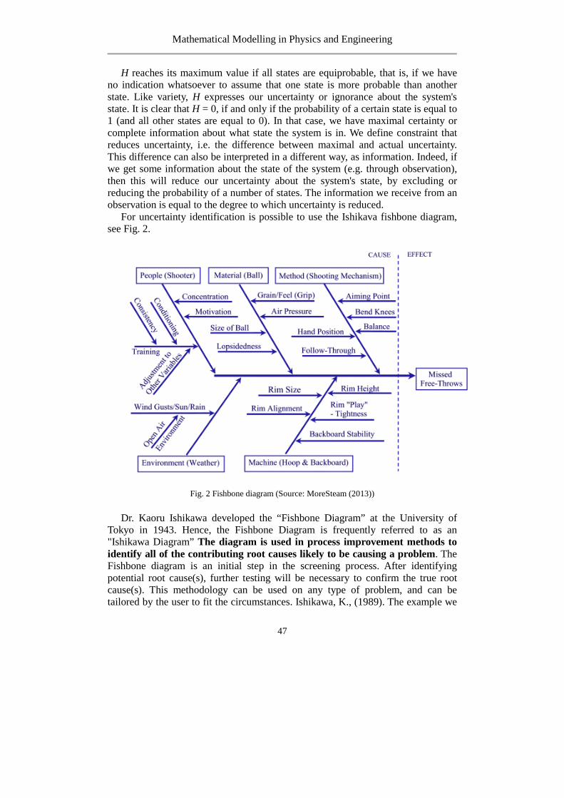
H reaches its maximum value if all states are equiprobable, that is, if we have no indication whatsoever to assume that one state is more probable than another state. Like variety, H expresses our uncertainty or ignorance about the system's state. It is clear that H = 0, if and only if the probability of a certain state is equal to 1 (and all other states are equal to 0). In that case, we have maximal certainty or complete information about what state the system is in. We define constraint that reduces uncertainty, i.e. the difference between maximal and actual uncertainty. This difference can also be interpreted in a different way, as information. Indeed, if we get some information about the state of the system (e.g. through observation), then this will reduce our uncertainty about the system's state, by excluding or reducing the probability of a number of states. The information we receive from an observation is equal to the degree to which uncertainty is reduced.
For uncertainty identification is possible to use the Ishikava fishbone diagram, see Fig. 2.
Fig. 2 Fishbone diagram (Source: MoreSteam (2013))
Dr. Kaoru Ishikawa developed the “Fishbone Diagram” at the University of Tokyo in 1943. Hence, the Fishbone Diagram is frequently referred to as an "Ishikawa Diagram” The diagram is used in process improvement methods to identify all of the contributing root causes likely to be causing a problem. The Fishbone diagram is an initial step in the screening process. After identifying potential root cause(s), further testing will be necessary to confirm the true root cause(s). This methodology can be used on any type of problem, and can be tailored by the user to fit the circumstances. Ishikawa, K., (1989). The example we
Mathematical Modelling in Physics and Engineering
48
have chosen to illustrate is "Missed Free Throws" (the one team lost an outdoor three-on-three basketball tournament due to missed free throws) MoreSteam (2013). In manufacturing settings, the categories are often: Machine, Method, Materials, Measurement, People, and Environment. In service settings, Machine and Method are often replaced by Policies (high-level decision rules), and Procedures (specific tasks).
2. Petri net
A gentle introduction into Petri nets modelling approach is made for example by WoPeD (WoPeD 2005) where Petri nets are described as follows: “Petri Nets are a graphical and mathematical modelling notation first introduced by Carl Adam Petri's dissertation published in 1962 at the Technical University Darmstadt (Germany). A Petri Net consists of places, transitions, and arcs that connect them. Places are drawn as circles, transitions as rectangles and arcs as arrows. Input arcs connect places with transitions, output arcs connect transitions with places. Places are passive components and model the system state. They can contain tokens, depicted as black dots or numbers. The current state of the Petri Net (also called the marking ) is given by the number of tokens at each place. Transitions are active components that model activities that can occur and cause a change of the state by a new assignment of tokens to places. Transitions are only allowed to occur if they are enabled, which means that there is at least one token on each input place. By occurring, the transition removes a token from each input place and adds a token to each output place. Due to their graphical nature, Petri Nets can be used as a visualization technique like flow charts or block diagrams but with much more scope on concurrency aspects. As a strict mathematical notation, it is possible to apply formal concepts like linear algebraic equations or probability theory for investigating the behaviour of the modelled system. A large number of software tools were developed to apply these techniques.
Examples of properties that are widely verified on Petri's networks are liveness, boundedness, reachability, fairness, and others. Verification of individual properties may be analytical (for basic classes of Petri nets) or have simulation character (for higher classes of Petri nets). The other way of development was to broaden the basic definition of the Petri nets so that their modelling power complies with specific requirements. Examples include timed and stochastic Petri nets, which allow refinement of individual states changes with deterministic (Dorda 2008, Zuberek, 1991, Holliday and Vernon, 1987) or stochastic (Ajmone Marsan, 1990)time considerations.
3. Example
As an example,according (Ibl and Čapek 2016), is presented a stochastic Petri net consists of 5 places and 5 transitions, see Fig. 3. The model contains the essential characteristic features that are included in the process model. These elements are, for example, the sequence (e.g., transition T4), AND-split (transition T1), AND-join (transition T6), XOR (transitions T6 and T5 or T6 and T3).
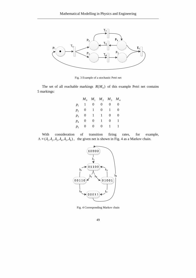
Mathematical Modelling in Physics and Engineering
49
Fig. 3 Example of a stochastic Petri net
The set of all reachable markings 0( )R M of this example Petri net contains 5 markings:
0 1 2 3 4
1
2
3
4
5
1 0 0 0 0
0 1 0 1 0
0 1 1 0 0
0 0 1 0 1
0 0 0 1 1
M M M M M
p
p
p
p
p
With consideration of transition firing rates, for example,
1 2 3 4 5 6Λ ( , , , , , )λ λ λ λ λ λ= , the given net is shown in Fig. 4 as a Markov chain.
Fig. 4 Corresponding Markov chain

Mathematical Modelling in Physics and Engineering
50
The solution of this chain, for ( )Λ 5,2,3,3,2,1= is stationary probability vector:
0.0385
0.2692
0.1538
0.3462
0.1923
η
=
The entropy of the example network can then be expressed by:
( ) 2
2 2
2 2
(0.0385log .0385
0.2692log 0.2692 0.1538log 0.1538
0.3462log 0.3462 0.1923log 0.1923) 2.093
0H SPN = −+ ++ + =
Reference limit (maximum entropy) is in this case is 2log 5 2.3219= − . The uncertainty for this particular case is determined by the relation
2 0( ) / log ( )H SPN R M− , i.e. 2.093 / 2.3219 0.9015= . This result can be loosely
interpreted as the fact that the uncertainty of the example stochastic Petri net (SPN) reaches 90.15%. Uncertainty can be then analysed as a response to changes in a parameter of SPN, for example, the number of tokens in the initial marking or an adjustment of a specific parameter λ ∈Λ . In the following is presented an example that shows the development of the uncertainty with a different initial marking. Fig. 5 indicates that the increasing number of tokens in the initial marking (in the place p1) decreases the uncertainty of SPN.
Fig. 5 Uncertainty vs. number of tokens
Unc
erta
inty
(SP
N)
M0(p1)
Mathematical Modelling in Physics and Engineering
51
4. Conclusion
Measurement of uncertainty can be an appropriate tool for assessing the relevance and the predictability of process models, and thus serve to more effective managerial decision making. The degree of uncertainty in the process model is directly dependent on two main indicators. The first is the number, the ratio and the distribution of specific elements (OR, XOR, AND, and LOOP) in the model. These elements provide branching, synchronization and cycles in the model, and thus are the main building blocks of process models that shape its specific structure. One of other approaches to the measurement of uncertainty in the process model (Jung et al., 2011)is based on quantifying the entropy of partial substructures of the model at different levels of abstraction. However, this approach takes into account only static structure of the model and does not take into account dynamic component, which can be expressed in Petri nets using tokens.
Keywords: uncertainty, entropy, modelling, stochastic Petri nets
References
[1] Ajmone Marsan M., Stochastic Petri nets: an elementary introduction. [in:] Advances in Petri nets, ed. Rozenberg G., Springer-Verlag, New York 1989.
[2] Brinkerhoff D., Ingle M., Integrating blueprint and process: a structured flexibility approach to development management, Public Administration and Development, 9(5), 1989, 487-503.
[3] Brugnach M., et al., Complexity and uncertainty: rethinking the modelling activity. [in:] Environmental modelling, software and decision support: state of the art and new perspectives, ed. A. J. Jakeman A. J., Voinov A. A., Rizzoli A. E., Chen S. H. Elsevier, Amsterdam 2008.
[4] Carpenter S. R., et al., Ecosystems and human well-being: scenarios‚ Millennium Ecosystem Assessment - MA (2005) project (eds.)‚ Island Press‚ Washington 2006.
[5] Dorda M., Introduction into Petri nets Retrieved from http://homel.vsb.cz/~dor028/Nekonvencni_metody_1.pdf, 2008.
[6] Hirschman A., The principle of the hiding hand, National Affairs, Issue 6, 1967. [7] Holliday M. A., Vernon M. K., A Generalized Timed Petri Net Model for Performance
Analysis. IEEE Transactions on Software Engineering, SE-13, 1987, 1297-1310. [8] Ibl M., Čapek J., Measure of Uncertainty in Process Models Using Stochastic Petri Nets and
Shannon Entropy. Entropy, 2016, 18, 33. [9] Ishikawa K., Introduction to Quality Control. Published by JUSE Press Ltd. Softcover reprint of
the hardcover 1st edition 1989 Distributed outside Japan and North America by: Chapman & Hall 2 -6 Boundary Row, London.
[10] Jung Y.-Y., Chin C.-H., Cardoso J., An entropy-based uncertainty measure of process models. Information Processing Letters, 2011, 111, 135-141.
[11] Moresteam, Retrived from https://www.moresteam.com/toolbox/fishbone-diagram.cfm, 2013. [12] Morgan D., Retrived from http://bvcentre.ca/files/research_reports/09-12-Morgan-Complexity-
Uncertainty.pdf, 2010. [13] Oberman W.L., et al., Error and uncertainty in modeling and simulation. Reliability
Engineering and System Safety 75, 2002, 333-357. [14] Root H., et al., Managing complexity and uncertainty in development policy. Retrieved from
https://www.researchgate.net/profile/Hilton_Root/publication/280884255_Managing_

Mathematical Modelling in Physics and Engineering
52
Complexity_and_Uncertainty_in_Development_Policy_and_Practice/links/55ca8b3d08aebc967dfbe5ca/Managing-Complexity-and-Uncertainty-in-Development-Policy-and-Practice.pdf, 2015.
[15] Simon H. A., Theories of bounded rationality [in:] Decision and organization, ed. McGuire C. B., Radner R., North-Holland Publishing Company, Amsterdam 1972.
[16] Sterman J. D., All models are wrong: Reflections on becoming a system scientist, [in:] Jay Wright Forrester Prize Lecture. Syst. Dyn. Rev. 18, 2002, 501-531.
[17] Van Den Belt M., Mediated Modeling: A System Dynamics Approach to Environmental Consensus Building. Island press, 339 pp., 2004.
[18] WoPeD, http://193.196.7.195:8080/woped/PetriNets, 2005. [19] Zuberek W. M., Timed Petri nets definitions, properties, and applications. Microelectronics
Reliability, 1991, 31, 627-644.

Mathematical Modelling in Physics and Engineering
53
MIXED-MODE LOAD TRANSFER IN THE FIBRE BUNDLE MODEL OF NANOPILLAR ARRAYS
Tomasz Derda
Institute of Mathematics, Czestochowa University of Technology, Czestochowa, Poland
The phenomena of failure and fracture of materials are a complex collection of phenomena in science and engineering. For the reason of the disorder in materials and their inherent nonuniformity, the failure processes of real materials usually cannot be described by simple linear equations. Therefore, statistical models are widely used to study the fracture and breakdown processes. One of the most important theoretical approaches is the fibre bundle model (FBM) [1-2], which illustrates a stochastic fracture-failure process in disordered materials subjected to external load. The crucial aspect of the FBM is a load transfer rule which is responsible for the mechanism of redistribution of load carried by the broken fibres (elements) to the intact ones. The load sharing rules can be divided into two extreme classes: global load sharing (GLS) and local load sharing (LLS). In the GLS model, long-range interactions are assumed as all the intact elements equally share a load of a failed element. The LLS model represents short-range interactions – the load from the destroyed element is redistributed only to its nearest intact neighbours. Both of these rules are idealised cases, hence Pradhan et al.[3] proposed mixed-mode load sharing rule and explored it for one-dimensional case.
In this work, using the mixed-mode FBM, we analyse damage processes in arrays of vertical nanopillars distributed on a flat substrate. Pillars are located at sites of two-dimensional lattices. Only regular arrangements are analysed.
Consider an array of N longitudinal pillars subjected to an axial external load. The existence of defects in actual materials plays a key role in the mechanical response of materials under load. Hence, pillar-strength-thresholds i
thσ , Ni ,..,2,1= are quenched random variables distributed according to Weibull distribution:
( )
−−=ρ
λσσ th
thP exp1 . (1)
The mixed-mode load transfer is as follows. When a pillar fails, fraction g of its
load is transferred locally and the rest (g−1 fraction) is distributed globally. Therefore, the mixed-mode load sharing is an interpolation mechanism between the GLS and LLS – 0=g corresponds to the GLS rule and 1=g represents pure LLS rule.

Mathematical Modelling in Physics and Engineering
54
Loading process is realized by two different (but also equivalent) procedures: sudden loading (application of finite force) and quasi-static loading. These two loading ways allows us to find crossover between GLS regime and LLS regime. In order to find crossover we study critical loads NFcc /=σ and probability of
breakdown bP under given load.
It is known that for the GLS rule cσ follows normal distribution, while for the
LLS rule the distribution of cσ can be well fitted by the skew normal distribution
(SND) with cumulative distribution function:
( ) 1erfc 2T ,
2 2cP
σ ξ σ ξσ αωω
− − = − −
. (2)
SND is a generalization of normal distribution for non-zero skewness. Distributions of cσ have been fitted to SND for different values of g . We have
observed that values of α are significantly closer to zero for 6.0≤g than for
7.0≥g . In addition, for 7.0≥g all values of α are negative. This suggest that
for the 6.0≤g the GLS mode dominates and for the 7.0≥g short range
interactions dominate, while ( )7.0,6.0∈g constitutes crossover.
Keywords: array of pillars, load transfer rule, probability a nd statistics, crossover, critical load
References
[1] Hansen A., Hemmer P. C., Pradhan S., The Fiber Bundle Model: Modeling Failure in Materials, Wiley 2015.
[2] Alava M.J., Nukala P.K.V.V., Zapperi S., Statistical models of fracture, Adv. Phys. 2006, 55, 349–476.
[3] Pradhan S., Chakrabarti B.K., Hansen A., Crossover behavior in a mixed-mode fiber bundle model, Phys. Rev. E 2005, 71, 036149.

Mathematical Modelling in Physics and Engineering
55
QUANTUM ENTANGLEMENT IN AVIAN NAVIGATION
Andrzej Drzewiński
Institute of Physics, University of Zielona Góra, Zielona Góra, Poland
The mechanism of in-flight navigation during the seasonal movement of migratory birds has been puzzling researchers for a long time. Since the early 1970s, there is evidence that birds are able to use the Earth’s magnetic field as their compass [1]. At present, there is a prevailing opinion that there are two types of magnetodetection: based on iron-containing structures in the beaks like for a homing pigeon or based on a chemical sensor in the bird’s eye like for the European Robin [2]. In the latter case, there is a hypothesis that these birds exploit the quantum correlations to navigate in Earth magnetic field. This phenomena could be based on magnetically sensitive chemical reactions in a bird eye. But how can it be reconciled with the facts that quantum effects, like superposition and entanglement, are easily destroyed by interaction with the environment? Generally, quantum phenomena have been observed at low temperatures in both microscopic and macroscopic systems. Presently, it seems that the effects can also occur at high temperatures if the systems are not in thermal equilibrium [3]. Decoherence due to contact with a hot environment typically restricts quantum phenomena to the low temperature limit, kBT/gμBB≪ 1 (gμBB is the single particle Zeeman energy where μB is the Bohr magneton, kB is the Boltzmann constant, and g is the Landé g-factor). But when a system is not in thermal equilibrium, the temperature no longer provides the relevant energy scale! The main parameters of the Earth’s magnetic field are inclination, declination and total intensity. The intensity is relatively very weak varying from about 30 μT near the equator to about 60 μT at the poles. But the avian magnetic compass was found to be an inclination compass based on the inclination of the Earth’s magnetic field lines instead of pointing to north or south. In 2000 Ritz et al. proposed a comprehensive model of chemical magnetoreception, so called, the Radical Pair Model [4]. European Robins are supposed to have a (blue) light-dependent magnetic compass based on the photochemical creation of radical pairs (two electrons located on different molecules) in photoactive pigment. It was proposed that the retinal cells of the bird eye seem to be the most suitable locations for the radical pair mechanism. Chemical reactivity of the radical pair is determined by the relative alignment of the two electron spins at any given time. Before radical pair of electrons recombines their correlated spins are in the superposition of singlet (SI) or triplet (TR) states. While both electron spins interact with the Earth’s magnetic field, one of them additionally interacts with a nuclear spin which leads to different local spin environments. Due to it coherent quantum oscillations between entangled singlet
Mathematical Modelling in Physics and Engineering
56
and triplet states appear and, moreover, their time evolution is very sensitive to the inclination of the molecule with respect to the Earth’s magnetic field. Therefore, one can expect that the rate constants kSI and kTR related do the decay of both states into a singlet or triplet state have different values, leading to different relative concentration of product states. In turn, a different concentration of both chemical products may modulate either sensitivity of photoreceptors or affect the light response of some cells. As a result light responses from different parts of the retina would be different depending on alignment of a photoactive cell relative to the magnetic field vector. In this way a visual pattern of light and shade, appearing in the bird's field of view, provides orientation information. The predictions of the radical-pair mechanism are consistent with many theoretical [5,6,7] and experimental results. For example, it has been verified that a very small oscillating magnetic field can disrupt the bird’s ability to orientate [8]. The duration of quantum entanglement in the bird’s eye is surprisingly long. It demonstrates that the evolution has preserved quantum effects to ensure optimization of some biological functions critical for survival [9]. It is also believed that the quantum avian compass can provide the foundation for a new generation of selective magnetic-sensing nano-devices.
Keywords: quantum mechanics, biological systems, model of avian magnetoreception
References
[1] Wiltschko W., Wiltschko R., Magnetic compass of European Robins, Science, 1972, 176, 62-64.
[2] Kishkinev D.A., and Chernetsov N.S., Magnetoreception Systems in Birds: A Review of Current Research, Biology Bulletin Reviews, 2015, 5, 46–62.
[3] Ball P., Physics of life: The dawn of quantum biology, Nature, 2011, 474, 272-274. [4] Ritz, T., Adem, S., & Schulten, K., A model for photoreceptor-based magnetoreception in birds,
Biophys J, 2000, 78, 707–718. [5] Pedersen J.B., Nielsen C., Solov’yov I.A., Multiscale description of avian migration: from
chemical compass to behaviour modeling, Sci. Rep., 2016, 6, 36709-1-12. [6] Hiscock H.G., Worster S., Kattnig D.R., Steers Ch., Jin Y., Manolopoulos D.E., Mouritsen H.,
and Hore P.J., The quantum needle of the avian magnetic compass, Proc. Natl. Acad. Sci. USA, 2016, 113, 4634–4639.
[7] Poonia V.S., Kondabagil K., Saha D., and Ganguly S., Functional window of the avian compass, Phys. Rev. E, 2017, 95, 052417-1-8.
[8] Zapka M., Heyers D., Hein Ch.M., Engels S., Schneider N-L., Hans J., Weiler S., Dreyer D., Kishkinev D., Wild J.M., and Mouritsen H., Visual but not trigeminal mediation of magnetic compass information in a migratory bird, Nature, 2009, 461, 1274–1277.
[9] Gauger E.M., Rieper E., Morton J.J.L., Benjamin S.C., Vedral V., Sustained Quantum Coherence and Entanglement in the Avian Compass, Phys. Rev. Lett. 2011, 106, 040503-1-4.

Mathematical Modelling in Physics and Engineering
57
FUNCTIONS OF BOUNDED VARIATION AND THEIR PROPERTIES
Oliwia Fertacz, Agata Paluszewska
Institute of Mathematics, Czestochowa University of Technology, Czestochowa, Poland
[email protected], [email protected]
In this paper we present the definition of total variation and show the most important properties and applications of bounded variation functions. The concept of bounded variation functions was first introduced by Camille Jordan (1838-1922). Many other mathematicians expanded this issue and showed a lot of applications of bounded variation functions in different fields of mathematics, i.a. calculus of variations, geometric measure theory, mathematical physics. Moreover, functions of bounded variation have a wide range of applications in calculus, particularly in Riemann–Stieltjes integral.
Definition 1
Let be a function defined on an interval [, ]. Let us part the given interval as follows: = < < ⋯ < = and determine the quantity
= sup !| # − #%|
#&,
where the supremum runs over all finite partitions ( of the interval [, ]. The quantity is called the total variation of on the interval [, ]. Definition 2
If < ∞, then the function is said to be of bounded variation on [, ]. Properties of bounded variation functions:
1. For any BV function we have
| b − a| ≤ .
2. A function of bounded variation on an interval [, ] is bounded on the given interval.
3. A sum, a difference and a product of bounded variation functions is a function of bounded variation.
4. Let : [, ] → / be a function of bounded variation and let 0 ∈ /. Then a function 0 is a function of bounded variation too. Furthermore
0 = |0| .
Mathematical Modelling in Physics and Engineering
58
5. A total variation is an additive function of the interval [, ], i.e.:
= 2 + 2 , where < 4 < .
6. If a function is bounded variation function on an interval [, ], then for any ≤ ≤ a total variation
5 = 6 7
is a bounded and increasing function of variable x.
In the further part of this work there are criteria for existence and uniqueness of bounded variation functions, relationship between functions of bounded variation and the other classes of functions (continuous functions, monotonic functions, lipschitz functions) and applications of bounded variation functions.
Keywords: mathematics, functions of bounded variation, total variation
References
[1] Fichtenholz G.M., Rachunek różniczkowy i całkowy, tom III, PWN, Warszawa 1963. [2] Kaczor W.J. Nowak M.T. , Zadania z analizy matematycznej 3, PWN, Warszawa 2006 [3] Natanson I.P, Theory of functions of a real variable, Frederick Ungar Publishing Company,
New York 1955. [4] http://www.theinfolist.com/php/SummaryGet.php?FindGo=bounded_variation

Mathematical Modelling in Physics and Engineering
59
ALGORITHM OF REBUILDING A BOUNDARY OF DOMAIN DURING CREATION OF AN OPTIMAL SHAPE
Katarzyna Freus1, Sebastian Freus2
1 Institute of Mathematics, Czestochowa University of Technology 2 Institute of Computer and Information Science, Czestochowa University of Technology
Czestochowa, Poland [email protected], [email protected]
In order to achieve the desired topology we often have to remove material of the area considered. This work presents the author's algorithm which can be used in the reconstruction of the boundary of domain after elimination of a certain amount of material. The paper presents some details concerning creating holes inside the area and removing the nodes. The topological-shape sensitivity method for the Laplace equation is used to obtain an optimal topology, whereas numerical methodology utilizes the boundary element method [1-4]. The topological derivative gives the information on the opportunity to create a small hole in the domain of interest. Wherever the value of topological derivative is low enough, the material can be eliminated. On the holes created via topological derivative, the Neumann boundary condition is prescribed. In order to find the desired optimal topology of the domain considered, the iterative procedure is used.
To check the effectiveness of the proposed algorithm, the example of computations is presented. The Laplace equation supplemented by the boundary conditions is taken into account (Fig. 1). The square domain of dimensions 0.1×0.1m is considered. Thermal conductivity equals λ=1 W/(mK). The boundary conditions are marked in Figure 1.
Fig. 1. Domain considered
The final result is obtained at iteration i=21, as can be seen in Figure 2.
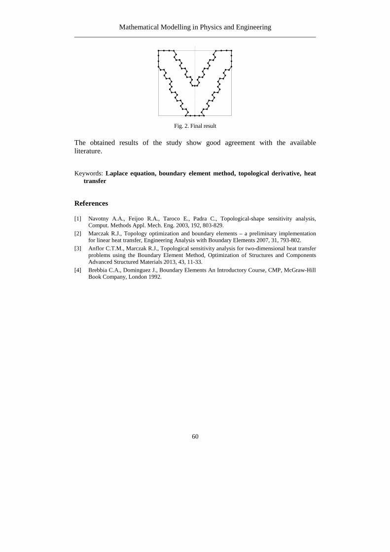
Mathematical Modelling in Physics and Engineering
60
Fig. 2. Final result
The obtained results of the study show good agreement with the available literature.
Keywords: Laplace equation, boundary element method, topological derivative, heat transfer
References
[1] Navotny A.A., Feijoo R.A., Taroco E., Padra C., Topological-shape sensitivity analysis, Comput. Methods Appl. Mech. Eng. 2003, 192, 803-829.
[2] Marczak R.J., Topology optimization and boundary elements – a preliminary implementation for linear heat transfer, Engineering Analysis with Boundary Elements 2007, 31, 793-802.
[3] Anflor C.T.M., Marczak R.J., Topological sensitivity analysis for two-dimensional heat transfer problems using the Boundary Element Method, Optimization of Structures and Components Advanced Structured Materials 2013, 43, 11-33.
[4] Brebbia C.A., Dominguez J., Boundary Elements An Introductory Course, CMP, McGraw-Hill Book Company, London 1992.

Mathematical Modelling in Physics and Engineering
61
A DESIGN OF AN OPTIMAL SHAPE OF DOMAIN DESCRIBED BY NURBS CURVES USING THE TOPOLOGICAL DERIVATIVE
AND BOUNDARY ELEMENT METHOD
Katarzyna Freus1, Sebastian Freus2
1 Institute of Mathematics, Czestochowa University of Technology 2 Institute of Computer and Information Science, Czestochowa University of Technology
Czestochowa, Poland [email protected], [email protected]
The goal of this paper is to create an optimal shape of the 2D domain that is described by the Non-Uniform Rational B-Splines (NURBS) curves. This work presents a method based on the topological derivative for the Laplace equation that determines the sensitivity of a given cost function (the total potential energy) to the change of its topology. The local value of the DT is defined as follows
0
( ) ( )( ) lim
( )TD xf
εε
ψ ψε→
Ω − Ω= (1)
where ( )ψ Ω and ( )εψ Ω are the cost functions calculated for the original Ω and the
new domain εΩ , respectively, and f is a regularizing function. In this work, the definition called the topological – shape sensitivity method is adopted
00
( ) ( )( ) lim
( ) ( )TD xf f
ε δε εεδε
ψ ψε δε ε
+
→→
Ω − Ω=
+ − (2)
where δε is a small perturbation on the radius of the hole. Topological optimization is a mathematical method that allows one to find an
optimal material layout of a domain, such that a cost function gives its optimum value after optimization under given constraints. Material is removed by creating a small hole that appears in the optimization process. The topological derivative (DT) indicates the position in the domain of interest where a hole should be formed. Wherever DT is low enough, a hole is created [1-4]. In the opening, the Neumann condition is taken into account. As a numerical approach, the boundary element method is considered in its direct version [5,6]. The boundary of the domain is described by the NURBS curves which are commonly used for representing and designing a shape in numerical implementation [7].
The following numerical example is considered
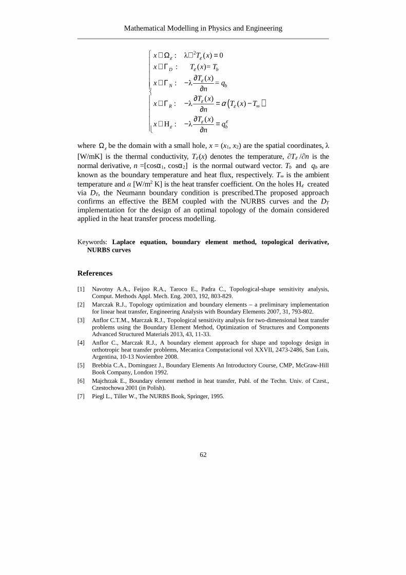
Mathematical Modelling in Physics and Engineering
62
( )
2: λ ( ) 0
: ( )=
( ): λ =
( )
: λ ( )
( )H : λ
D b
N b
R
b
x T x
x T x T
T xx q
nT x
x T x Tn
T xx q
n
ε ε
ε
ε
εε
εεε
α ∞
∈Ω ∇ = ∈Γ ∂∈Γ − ∂
∂ ∈Γ − = − ∂
∂ ∈ − = ∂
where εΩ be the domain with a small hole, x = (x1, x2) are the spatial coordinates, λ
[W/mK] is the thermal conductivity, Tε (x) denotes the temperature, ∂Tε /∂n is the normal derivative, n =[cosα1, cosα2] is the normal outward vector. Tb and qb are known as the boundary temperature and heat flux, respectively. T∞ is the ambient temperature and α [W/m2 K] is the heat transfer coefficient. On the holes Hε created via DT, the Neumann boundary condition is prescribed.The proposed approach confirms an effective the BEM coupled with the NURBS curves and the DT implementation for the design of an optimal topology of the domain considered applied in the heat transfer process modelling.
Keywords: Laplace equation, boundary element method, topological derivative, NURBS curves
References
[1] Navotny A.A., Feijoo R.A., Taroco E., Padra C., Topological-shape sensitivity analysis, Comput. Methods Appl. Mech. Eng. 2003, 192, 803-829.
[2] Marczak R.J., Topology optimization and boundary elements – a preliminary implementation for linear heat transfer, Engineering Analysis with Boundary Elements 2007, 31, 793-802.
[3] Anflor C.T.M., Marczak R.J., Topological sensitivity analysis for two-dimensional heat transfer problems using the Boundary Element Method, Optimization of Structures and Components Advanced Structured Materials 2013, 43, 11-33.
[4] Anflor C., Marczak R.J., A boundary element approach for shape and topology design in orthotropic heat transfer problems, Mecanica Computacional vol XXVII, 2473-2486, San Luis, Argentina, 10-13 Noviembre 2008.
[5] Brebbia C.A., Dominguez J., Boundary Elements An Introductory Course, CMP, McGraw-Hill Book Company, London 1992.
[6] Majchrzak E., Boundary element method in heat transfer, Publ. of the Techn. Univ. of Czest., Czestochowa 2001 (in Polish).
[7] Piegl L., Tiller W., The NURBS Book, Springer, 1995.

Mathematical Modelling in Physics and Engineering
63
THE USE OF THE IMAGE PROCESSING AND ANALYSIS METHODS FOR OPTIMIZATION OF EQUATIONS OF MOTION
FOR A QUADRUPED ROBOT
Katarzyna Gospodarek
Institute of Computer and Information Science, Czestochowa University of Technology, Czestochowa, Poland
This paper discusses some of the issues related to the implementation of the software which is responsible for the gait generation process for simple four-legged walking machine. It has been suggested to use additional software elements, include those which allow to track the position of the key points of the structure during its movement and to use of collected data to implement the appropriate correction factors. The analysed quadruped walking machine is shown in Fig. 1. The main functionality of the additional software module was based on methods and algorithms related to image processing and analysis. The vision analysis was conducted in two steps. The first step was focused on the study of the correctness of transfer of motion by the system of links used in the limbs of the robot. While the second one was responsible for verifying the movement of the whole machine.
Fig. 1. Design of the analysed quadruped robot
The gait generation process of the any walking machine is closely related to its type. The parameters that allow its appropriate movement are selected depending on the number of limbs and the type of gait. In the case of simple walking constructions, the basic gait type is creep, also referred to as mechatronic walking. In general, these names refer to the gait of each device, whose construction is always supported by min. N-1 limbs during its motion [1].
During the integration of software responsible for gait generation process with the real model of robot often discloses the influences other factors such as uncertainty in robot construction or the complicated geometry of the limbs [2]. One of the key factors that can interfere with the robot gait generation process is for example, type of connection of the control motors with degrees of freedom [1].

Mathematical Modelling in Physics and Engineering
64
The methods and algorithms provided by the OpenCV video library were used to identify the motion parameters and the irregularities that occurred during it. Software module that was implemented allows cooperation with both the already registered video material and that the intercepted in real-time. Its basic functionality is primarily associated to finding the current position of the specific points of the construction. The additional elements are responsible for the transmission of data information and the factors calculated on the basis of their value to control system of machine. The schematic representation of this process is illustrated in fig. 2.
Fig.2 The schematic representation of additional software
In order to simplify the process of identifying the selected points, each of them was accompanied by additional marker with a unique color. During the work on the implementation of software it was decided to use the CAMShift (Continuously Adaptive Meanshift ) algorithm as a method that is responsible for tracking the displacement of the key elements. Due to the fact that the CAMShift algorithm is based on the definition on finding of local extreme in the density distribution of the data set, the basis for object detection is its color, and more specifically, the histogram that was built for its color space [3, 4]. An accurate theoretical description of the algorithm, its mathematical dependencies, and assumptions about the use of the histogram as one of the simplest density estimators have been fully explained in many publications, see [3, 4, 5, 6].
In the first phase of the tests the correctness of the angles obtained by the joints of the robot was verified. At this step, the values of the angles given by the software which was controlled the movement of the limb were compared to the values obtained by the joints in fact. The results of the tests are shown in Fig. 3a. In order to eliminate any discrepancies, the software that was used has been extended to communicate with the control system of walking machine. Its functionality was based on the feedback loop mechanism, which allowed a significant correction of the results, as shown in Fig. 3b.

Mathematical Modelling in Physics and Engineering
65
Fig. 3. The relationship between the pre-set and read value for joint variable θ2 (knee joint of the structure), a) before correction, b) after correction
Further analyzes was related to video feedback used to correct movement of the whole structure. The research was based on the use of appropriate correction factors to ensure the maintenance of the specified motion by the quadruped robot. In this case, the specific points which were tracking were located on the back of the construction.
Keywords: image processing, CAMShift, quadruped robot
References
[1] Zielińska T.: Maszyny kroczące. Warszawa: Wydawnictwa Komunikacji i Łączności, 2005. [2] Tchoń K., Mazur A., Dulęba I.: Manipulatory i roboty mobilne. Modele, planowanie ruchu,
sterowanie. Warszawa: Akademicka Oficyna Wydawnicza PLJ, 2000. [3] Bradski G., Kaehler A.: Learning OpenCV. Computer Vision with the OpenCV Library.
Sebastopol, CA: O'Reilly Media, 2008. [4] Joshi S., Gujarathi S., Mirgemoving A.: Moving Object Tracking Method Using Improved
Camshift With Surf Algorithm. „International Journal of Advances in Science Engineering and Technology”, 2014, 2, 2.
[5] Allen J. G., Xu R. Y. D., Jesse S. J.: Object Tracking Using CAMShift Algorithm and Multiple Quantized Feature Spaces. „Proceedings of the Pan-Sydney area workshop on Visual information processing”, 2004, 3-7.
[6] Comaniciu D., Ramesh V., Meer P.: Kernel-Based Object Tracking. „IEEE Transactions on Pattern Analysis and Machine Intelligence”, IEEE Transactions on, 2003, 564-577.

Mathematical Modelling in Physics and Engineering
66

Mathematical Modelling in Physics and Engineering
67
PEGCPP: AN EFFICIENT IMPLEMENTATION OF PARSER GENERATOR IN C++
Andrzej Grosser, Grzegorz Michalski
Institute of Computer and Information Sciences, Czestochowa University of Technology, Czestochowa, Poland
[email protected], [email protected]
Parsing expression grammars (pegs) is an alternative notation to BNF [1]. The basic difference between these notations results from the way, in which the alternative is implemented. In the case of the parsing expression grammar alternatives are ordered. Prior alternatives have a higher priority in choosing from later ones. In this way, the description of language using pegs is always unambiguous. By using pegs it is possible describing all the context-free languages and even some context-sensitive languages.
The parsing expression grammar can easily be translated into a parser by using the recursive descent method. However, there is a problem with backtracking. When one of the alternatives fails, it is necessary to consider the next one, which may require a recalculation. It is possible to apply memoization of previous calculations, thus reducing the computational complexity to linear [2]. It is also possible to make pegs using a parser machine [3].
Translators using parsing expressions have been implemented in many programming languages, including C++ [4,5,6]. C++ implementations use templates and overloading operators. In this way, the description of the language are implemented directly in the code of the translator program. However, there is a problem with the understanding of the description, since it needs an adaptation the notation of parsing expressions to C++ syntax. In addition, the compiler messages associated with advanced metaprogramming can be obscure.
The implementation described in this article is based on converting the specification language script to the C ++ source code. This way, the language description is clear and can be build high performance parser. By separating the description of the parser from its executable form is possible to support the language designer with the tools built into the specification language translator. The generated parser code is syntactically correct, so the language designer does not need to look C++ compiler error messages. The generated code can include optimizations related to the advanced capabilities of C++.
Keywords: parser generator, parsing expression grammar, high performance, C++

Mathematical Modelling in Physics and Engineering
68
References
[1] Ford, B: Parsing Expression Grammars: A Recognition-Based Syntactic Foundation, Proceedings of the 31st ACM SIGPLAN-SIGACT Symposium on Principles of Programming Languages, POPL 2004, ACM, Venice, Italy, 14–16 January 2004.
[2] Ford, B: Packrat Parsing: Simple, Powerful, Lazy, Linear Time, International Conference on Functional Programming, October 4-6, 2002, Pittsburgh
[3] Medeiros, S., Ierusalimschy, R.. A parsing machine for PEGs. In: DLS ’08: Dynamic languages Symposium. New York, USA: ACM.
[4] Spirit http://www.boost.org/doc/libs/1_64_0/libs/spirit/doc/html/index.html [5] Cpp-peglib https://github.com/yhirose/cpp-peglib [6] Pegtl https://github.com/taocpp/PEGTL

Mathematical Modelling in Physics and Engineering
69
REPRESENTATIONS OF RIGHT HEREDITARY TENSOR ALGEBRAS OF BIMODULES
Nadiya Gubareni
Institute of Mathematics, Czestochowa University of Technology, Czestochowa, Poland
In this talk we present some results from representation theory of right hereditary tensor algebras of bimodules. The methods of representation theory of such algebras allows to classify right hereditary semiperfect semidistributive (SPSD) rings of bounded representation type.
We consider O-species that are a special case of species as was introduced by Yu.A. Drozd [3]. Let Oi be a family of discrete valuation rings (not necessarily commutative) with Jacobson radical Ri and skew fields of fractions Di for i = 1,2,...,k oraz Dj a family of skew fields for j = k+1, ...,n. Then we can form an O-species Ω = (Ai, iMj), where all Ai = )( in OH
iare prime hereditary Noetherian
semiperfect rings or Ai, and all iMj are )~~
( ji AA − -bimodules, as shown in [4]. If
all skew fields Di (for i =1,2,...,n) are the same skew field D an O-species is said to be (D,O)-species.
With an O-species Ω we can associate the quiver Γ(Ω) as the directed graph whose vertices are indexed by the numbers i = 1, 2,..., n and there is an arrow from the vertex i to the vertex j if and only if iMj ≠ 0. We also associate a tensor
algebra Τ(Ω) to an O-species Ω = (Ai, iMj) in the following way. Let ∏=
=n
iiAB
1
,
and ji
n
jiMM
1, =⊕= . Then B is a ring and M is a (B,B)-bimodule. Then the ring
,)(0
ii
B TMT∞
=⊕=
where T0 = B, and Ti+1 = Ti ⊗B M ( i > 0) with component-wise addition and the multiplication induced by taking tensor products, is called the tensor algebra of the species Ω. We study the connections between the representations of O-species and modules over the corresponding tensor algebra. We give the conditions on (D, O)-species and right hereditary tensor algebra Τ(Ω) to be of bounded representation type in the sense of R.B. Warfield Jr. [6] and V. Dlab, C.M. Ringel [1], [2]. We give the description of such (D,O)-species in terms of Dynkin diagrams and diagram with weights similar to [4]. We also study the connections of
Mathematical Modelling in Physics and Engineering
70
such (D,O)-species and tensor algebras with right hereditary SPSD-rings and give the description of these rings of bounded representation type.
In this talk we discuss the solving matrix problems over discrete valuation rings and skew fields, which are a generalization of matrix problems considered in [7]. These matrix problems, i.e. the problems of reducing a family of matrices by some family of admissible transformations, arise in the natural way as in linear algebra in studying the representations of (D,O)-species and modules over tensor algebras. The solving such matrix problems considered in [5] is the main method to obtain the results of our talk.
Keywords: representation theory, tensor algebra of bimodule, species, hereditary rings, mixed matrix problems, discrete valuation rings, rings of bounded representation type
References
[1] Dlab V. and Ringel C.M., On algebras of finite representation type, J. Algebra, 1975, 33(2), 306-394.
[2] Dlab V. and Ringel C.M., Indecomposable representations of graphs and algebras, Mem. Amer. Math. Soc., 1976, 173.
[3] Drozd Yu.A., The structure of hereditary rings, Math. USSR Sbornik, 1982, 41(1), 139-148. [4] Gubareni N., Tensor algebras of bimodules and their representations, Sarajevo Journal of
Math., 2016, 12 (25), 2, 357-372, Suppl. [5] Gubareni N., Some mixed matrix problems over several discrete valuation rings, J. Appl. Math.
Comput. Mech., 2013, 4(12), 47-58. [6] Warfield R.B., Serial rings and finitely presented modules, J. Algebra, 1975, 37(2), 187-222. [7] Zavadskij A.G., Revitskaya U.S., A matrix problem over a discrete valuation ring, Sbornik:
Mathematics, 1999, 190(6), 835-858.

Mathematical Modelling in Physics and Engineering
71
MODELING OF MECHANICAL PHENOMENA IN THE PLATINUM-CHROMIUM CORONARY STENTS
Aneta Idziak-Jabłońska 1, Karolina Karczewska 2,Olga Kuberska2
1 Institute of Mechanical Technology, Czestochowa University of Technology, 2 Student Scientific Society of Biomedical Engineering, Institute of Mechanical Technology,
Czestochowa University of Technology, Czestochowa, Poland
[email protected], [email protected], [email protected]
This study discusses the geometrical model of a coronary stent with known design and strength analysis using the finite element method. The coronary stent model was made of platinum and chromium alloy. Static analysis based on compression of the coronary stent was also performed. The aim of the analysis was to examine strength of the stent structure. The study analyzed stresses, displacements and plastic strains after applying a constant load to the stent walls. The mechanical phenomena such as percentage degree of shortening (foreshortening), relative narrowing and area of stent covering were also determined.
One of the biggest successes in the field of invasive cardiology was to use endovascular implants termed stents. These implants are designed as small metal wirings with cylindrical design. They are implanted in the location of the narrowed coronary artery in order to expand it and support the arterial walls [1].
Compared to stainless steel (surgical steel 316L), platinum-chromium alloy used in this study allows for a reduction in bending resistance and has better fit. The PtCr alloy is characterized by greater density compared to surgical steel 316L. Therefore, it is more visible in X-ray images despite smaller components in the stent. Studies have also shown that stents made of platinum-chromium alloys are faster covered by the neointima. Its flexibility allows for easier movement through the arteries without causing damages.
Conditions that characterize endovascular implants are: - longitudinal shortening after expansion of the stent is presented as a percentage
degree of shortening. The dimensions of the stents can be modified (shortened) during stent implantation, which has an effect on the final stent length. Knowledge of the shortening parameters is useful in choosing the adequate stent length and using it in the right position in human body [2].
89:;<ℎ9:7;>?>5 = @%@ABCD@ ∙ 100% (1)
where: L – initial stent length, IJK – stent length at the highest loaded. - relative narrowing (normal strain) - narrowing of the stent diameter caused by
compression related to its initial diameter. It is defined as:

Mathematical Modelling in Physics and Engineering
72
/;L7?M; >::9N?>5 = OP%OOP (2)
where: – initial stent diameter before compression, D - the smallest stent diameter after compression.
The geometrical model of the stent was developed using the SolidWorks 2014 software. With regard to its shape, the stent is numbered among net stents. A solid grid composed of 91052 nodes and 35711 elements was created for the stent model. The coronary stent model was made of platinum and chromium alloy. In order to perform numerical analysis, apart from the adopted material properties, it is also important to define boundary conditions. For this purposes, the stent model was fixed at its two ends. It is necessary to reduce the initial diameter of the implant in order to ensure proper implantation of the stent in the position of the artery narrowing. Furthermore, an insignificant diameter reduction protects from the possibility of removing from the catheter surface. The aim of the study is to evaluate the stent compression strength. It was adopted that the surgeon acts with a specific force on the external stent surface. Therefore, the stent model was loaded on both ends with the force of 10 N on four external walls. Stent model with applied forces and fixation is presented in Fig. 1.
Fig. 1. Stent model with applied forces and fixation
The statistical analysis performed using the finite element method allowed for evaluation of stent strength. The stent structures which are the most exposed to risk of damage during model compression were demonstrated. The study showed that an important aspect of stent design is adequate choice of material and model geometry.
Keywords: computational mechanics, FEM, mathematics, PtCr stent, SolidWorks
References
[1] Paszenda Z., Stenty w kardiologii interwencyjnej. Wybrane Zagadnienia, Wydawnictwo Politechniki Śląskiej, Gliwice, 2013.
[2] Idziak-Jabłońska A., Modelowanie zjawisk mechanicznych w stentach wieńcowych na podstawie analizy numerycznej, Mechanik, vol. 7, 2015, str. 303-310

Mathematical Modelling in Physics and Engineering
73
AN INFLUENCE OF A ROD OF A VARIABLE CROSS-SECTION AS A PART OF GEOMETRICALLY NONLINEAR COLUMN
SUBJECTED TO THE SPECIFIC LOAD ON A VALUE OF BIFURCATION LOAD
Anna Jurczyńska, Janusz Szmidla
Institute of Mechanics and Machine Design Fundamentals, Czestochowa University of Technology, Czestochowa, Poland
[email protected], [email protected]
Presented paper includes a theoretical considerations and a results of a numerical simulations concerning the issue of stability of slender geometrically nonlinear column with an element of variable cross-section subjected to the follower force directed towards the positive pole. The study focused on the influence of rod of variable cross-section on the value of bifurcation load corresponding to the loss of rectilinear form of static equilibrium of the considered system. Within the framework of the numerical simulations a phenomenon of local loss of rectilinear form of static equilibrium was analysed.
Geometrically nonlinear column is built of three prismatic rods [1] connected by an element ensuring an equality of deflections and angles of deflection at the free end of the system. Giving the assumption of known and constant total flexural stiffness of the column, a distribution of flexural stiffness is described by the coefficient of asymmetry of the flexural stiffness µ defined as follow:
( )
( )∑=
= III
Ikk
II
EJ
EJµ (1)
In a target system of the geometrically nonlinear column with the nonprismatic element analysed in this paper, the rod of lower flexural stiffness was replaced by the rod of variable cross-section and the same total volume resulting from the value of coefficient of asymmetry of the flexural stiffness µ. The variable cross-section was modelled by division of the rod into n prismatic segments of identical length and variable width, whereas an approximation of the shape by means the of linear function and a polynomial of degree 2 is considered. The columns were subjected to the follower force directed towards the positive pole which is one of the cases of specific load defined by L. Tomski [2].
O the basis of a such defined physical model of the geometrically nonlinear system with the element of variable cross-section, a total potential energy was determined. Taking into account known a priori the geometrical boundary conditions and the geometrical continuity conditions, a differential equations of displacement were determined as well as missing natural boundary conditions and

Mathematical Modelling in Physics and Engineering
74
continuity conditions. Due to the existing in the system geometrical nonlinearity, the boundary problem was solved using the small parameter method [3]. Taking into consideration the determined equations describing the analysed system, a numerical programmes enabling the analysis of the stability of the column were developed.
Fig. 1. The physical model of the system under the follower force directed towards the positive pole a) the geometrically nonlinear column, b) the geometrically nonlinear
column with the element of variable cross-section c) the model of the nonprismatic rod
Within the numerical calculations, an influence of rod of variable cross-section as a component of the geometrically nonlinear column with the nonprismatic element on the value of the bifurcation load corresponding to the loss of rectilinear form of static equilibrium. The phenomenon of an ‘exit’ from the region of the local loss of rectilinear form of static equilibrium was also analysed.
Keywords: slender system, specific load, nonprismatic, stability
References
[1] Tomski L., Uzny S., Drgania swobodne i stateczność wspornikowych kolumn geometrycznie nieliniowych poddanych obciążeniu swoistemu, rozdz. 6: Drgania swobodne i stateczność obiektów smukłych jako układów liniowych lub nieliniowych, praca zbiorowa pod kierunkiem naukowym i redakcją Lecha Tomskiego, Wydawnictwa Naukowo-Techniczne, Warszawa, 2007, pp. 173-218.
[2] Tomski L., Układy smukłe w aspekcie konserwatywnego i niekonserwatywnego obciążenia czynnego I biernego, rozdz. 1: Drgania swobodne i stateczność obiektów smukłych jako układów liniowych lub nieliniowych, praca zbiorowa pod kierunkiem naukowym i redakcją Lecha Tomskiego, Wydawnictwa Naukowo-Techniczne, Warszawa 2007, pp. 17-46.
[3] Szmidla J., Drgania swobodne i stateczność układów smukłych poddanych obciążeniu swoistemu, Wydawnictwo Politechniki Częstochowskiej, Seria Monografie, nr 165, Częstochowa 2009.

Mathematical Modelling in Physics and Engineering
75
ON TWO-PARAMETER FELLER SEMIGROUP WITH NONLOCAL CONDITION FOR ONE-DIMENSIONAL DIFFUSION
PROCESS
Bohdan Kopytko 1, Roman Shevchuk 2 1Institute of Mathematics, Czestochowa University of Technology,
Czestochowa, Poland 2Vasyl Stefanyk Precarpathian National University,
Ivano-Frankivsk, Ukraine [email protected], [email protected]
We consider the problem of construction of Feller semigroup associated with one-dimensional inhomogeneous diffusion process with membrane placed at the point, which location on real line is determined by the given function that depends on time variable. It is assumed that at the interior points of half-lines separated by membrane the desired process coincides with the ordinary diffusion processes given there and its behavior at the common boundary of these domains is described by the nonlocal Feller-Wentzell conjugation condition of non-transversal type [1-3]. This problem is often called the problem of pasting together two diffusion processes on a line [4, 5].
The study of the problem is performed by analytical methods. Such an approach allows to determine the desired semigroup by means of the solution of the corresponding problem of conjugation for a linear parabolic equation of the second order (backward Kolmogorov equation) with discontinuous coefficients [4-6]. A classical solvability of this problem is established under the assumption that the equation coefficients satisfy the Holder condition with nonzero exponent, the initial function is bounded and continuous on the whole real line and the parameter which characterize Feller-Wentzell conjugation condition and curve which determines the common boundary of domains where the equation is given satisfy Holder condition with exponent bigger than ½. In the course of investigation of the problem we use the fundamental solutions of parabolic equations and heat potentials associated with them [4-9]. As a result of their application the problem formulated above is being reduced to the system of two integral singular equations of Volterra of the second kind which solution is obtained by the method of successive approximations.
Note that the similar problem was considered earlier in work [6] in case the membrane was placed at a fixed point of the real line. We also mention works [10, 11] where the results concerning the problem of construction of diffusion processes with jumps at points of the boundary of the domain were obtained by the methods of functional [10] and stochastic [11] analysis.
Mathematical Modelling in Physics and Engineering
76
Keywords: diffusion process, nonlocal conjugation condition, parabolic potential
References
[1] Feller W., The parabolic differential equations and associated semigroups of transformations, Ann. of Math. Soc. 1952, 55, 468-519.
[2] Wentzell A.D., Semigroups of operators that correspond to a generalized differential operator of second order, Dokl. AN SSSR 1956, 111, 2, 269-272.
[3] Langer H., Schenk W., Knotting of one-dimensional Feller process, Math. Nachr. 1983, 113, 151-161.
[4] Portenko M.I., Diffusion Processes in Media with Membranes, Institute of Mathematics of the NAS of Ukraine, Kyiv 1995.
[5] Kopytko B.I., Sewing two nonhomogeneous diffusion processes on a straight line, Ukrainian Math. Journal 1983, 35, 2, 135-141.
[6] Shevchuk R.V., Pasting of two one-dimensional diffusion processes, Annales Mathematicae et Informaticae 2012, 39, 225-239.
[7] Pogorzelski W., Etude de la solution fondamentale de l’équation parabolique, Richerce Matem. 1956, 5, 25-57.
[8] Ladyzhenskaya O.A., Solonnikov V.A., Ural’tseva N.N., Linear and Quasilinear Equations of Parabolic Type, Nauka, Moscow 1967.
[9] Kamynin L.I., A boundary value problem in the theory of heat conduction with a nonclassical boundary condition, Comput. Math. Math. Phys. 1964, 4, 6, 33-59.
[10] Skubachevskii A.L., On Feller semigroups for multidimensional diffusion processes, Dokl. AN 1995, 341, 2, 173-176.
[11] Pilipenko A.Yu., On the Skorokhod mapping for equations with reflection and possible jumplike exit from a boundary, Ukrainian Math. J. 2012, 63, 9, 1415-1432.

Mathematical Modelling in Physics and Engineering
77
MODELLING OF HEAT CONDUCTION IN A COMPOSITE SPHERE USING FRACTIONAL CALCULUS
Stanisław Kukla, Urszula Siedlecka
Institute of Mathematics, Czestochowa University of Technology, Czestochowa, Poland
[email protected], [email protected]
The subject of this consideration is an analysis of the effect of fractional order of time-derivatives occurring in fractional heat conduction models on the temperature distribution in a composite consisting of inner solid sphere and a spherical layer (Fig. 1) [1]. The time-fractional heat conduction is governed by the following differential equation
22
1 1, 1,2
i
i
i i
i
T Tr i
r r r a t
α
α∂ ∂∂ = = ∂ ∂ ∂
(1)
where iλ is thermal conductivity, ia is thermal diffusivity and iα denotes the fractional order of the left-sided Caputo derivative with respect to time t .
Fig. 1. A cross-section of the sphere under consideration
We assume the condition at the centre of the solid sphere, the continuity conditions at the interface, the Robin boundary condition on the outer surface and the initial condition in the following form
( )0,T t < ∞ (2)
( ) ( )1 1 2 1, ,T r t T r t= (3)
( ) ( )1 21 11 21 1 2 1, ,RL RL
T TD r t D r t
r rβ βλ λ− −∂ ∂=
∂ ∂ (4)
( ) ( ) ( )( )21 22 2, ,RL
TD b t a T t T b t
rβλ −
∞ ∞∂ = −∂
(5)
r1
b
Mathematical Modelling in Physics and Engineering
78
( ) ( ),0 iT r F r= (6)
where T∞ is the ambient temperature, a∞ is the outer heat transfer coefficient and
iβ denotes the fractional order of the left-sided Riemann-Liouville derivative. To obtain the fractional equation with a constant coefficient, we introduce new
functions ( ),iU r t given by the formula
( ) ( ) ( )( ), , , 1,2i iU r t r T r t T t i∞= − = (7)
The boundary-initial problem (1-6) for functions ( ),iU r t was solved under so
called mathematical formulation - 1 2 1β β= = and physical formulation - 1 1β α= ,
2 2β α= [2]. An analytical solution of the time-fractional heat conduction problem under
mathematical conditions for 1 2α α α= = was determined by using the method of variables separation, in the form of appropriate eigenfuction series.
A solution of the considered problem under physical boundary and continuity conditions was determined by using the Laplace transform method, using of the Gaver algorithm to numerical inversion of the Laplace transform. The effect of the order of the fractional derivative on the temperature distribution in the sphere has been determined numerically.
Keywords: fractional heat conduction, Caputo and Riemann-Liouville derivatives
References
[1] Kukla S., Siedlecka U., Fractional heat conduction in a sphere under mathematical and physical Robin conditions, submitted to Journal of Theoretical and Applied Mechanics.
[2] Povstenko Y., Time-fractional heat conduction in an infinite medium with a spherical hole under Robin boundary condition, Fractional Calculus and Applied Analysis, 16(2), 2013, 354-369.

Mathematical Modelling in Physics and Engineering
79
COMPARISON OF FREAK AND SURF ALGORITHMS FOR RECOGNIZING KEY ELEMENTS FOR TIME-VARYING IMAGES
Joanna Kulawik
Institute of Computer and Information Sciences, Czestochowa University of Technology, Czestochowa, Poland
Object recognition in time-varying images is now a rapidly evolving field of image processing. Detection of reference objects in a complex image is thought to be the basis of modern autonomous systems, especially in the automotive and military industries. Such a operations are complex and difficult to perform, and at the same time they require a high degree of reliability, which is often associated with the life and health of the person. Unfortunately, quality of the examined images are have high impact on detection efficiency [1, 2]. The conditions under which the pictures were taken are very significant [3]. Particularly important elements are included difficult lighting conditions, changing resolution (image accuracy), and image scaling and rotation. These elements are always present in time-varying images being analyzed in real time. Therefore, the purpose of the work was to investigated how big influence they had the mentioned difficulties on detect key elements in subsequent frames of the film are. Because of the need for real-time image analysis (e.g., motion detection in a moving mechanical vehicle), the complexity of time algorithms is also shown. Due to the large number of complicated numerical calculations, it is often a critical element of recognition systems.
In order to carry out the research, a reference image with the object of interest and images containing the sought object was prepared. The set of search images were consisted: images with photometric deformation - different luminance, images of different resolutions, images with geometric deformations - rotation, offset and scaling.
The analysis involves is of algorithms for constructing descriptors used: Fast Retina Key point (FREAK) algorithm [4] and SPEEDED-UP ROBUST FEATURES (SURF) algorithm [5, 6]. These are fairly new and effective algorithms in relation to older solutions such as SIFT [7]. Both methods are characteristic descriptors built for key elements. Positions of key points must be to set in advance. That's why, the FREAK algorithm is based on the characteristic points defined by the Harris & Stephens method [8], while the SURF algorithm has its own method. For both methods the input images were prepared in the same way - they were converted into monochrome [9], and next were them normalized to the scope 0-255 [9].
The last step was to carry out the proper detection based on the obtained descriptors in the first method and second method. For a built base was done

Mathematical Modelling in Physics and Engineering
80
comparison: detection of points of interest, sensitivity to changes in perspective, sensitivity to lighting conditions, influence of background texture and object sought on search precision were compared. For the analyzed cases, graphs of the dependence of the search efficiency on the scale change, and extraction time on the number of characteristic points were also determined.
Keywords: corner detection, object detection, feature detection, descriptors
References
[1] Forczmański P., Dziurzański P., System-level hardware implementation of simplified Low-Level color image descriptor, Proceedings 8th International Conference On Computer Recognition Systems CORES 2013, Advances in Intelligent Systems and Computing, vol. 226 (2013), pp. 461-468.
[2] Forczmański P., Markiewicz A., Two-stage approach to extracting visual objects from paper documents, Machine Vision and Applications, Volume 27 (2016), Issue 8, pp 1243–1257.
[3] Forczmański P., Kukharev G., Shchegoleva N., 2012, An algorithm of face recognition under difficult lighting conditions, Przegląd Elektrotechniczny (Electrical Review), r. 88 No. 10b/2012, pp. 201-204.
[4] Alahi A., Ortiz R., and Vandergheynst P.. Freak: Fast retina key point. In CVPR, 2012. 2. [5] Bay H., Tuytelaars T., Van Gool L., SURF: Speeded-up robust features, [w:] Lecture Notes in
Computer Science, t. 3951 (2006), pp. 404-417. [6] Bay H., Ess A., Tuytelaars T., Van Gool L., SURF: Speeded-Up Robust Features, [w:]
Computer Vision and Image Understanding (CVIU), t. 110 (2008), pp. 346-359. [7] Lowe, David G. (1999). "Object recognition from local scale-invariant features". Proceedings of
the International Conference on Computer Vision. 2. pp.1150-1157. doi:10.1109/ICCV.1999.790410.
[8] Harris C. and Stephens M., "A combined corner and edge detector" . Proceedings of the 4th Alvey Vision Conference, 1988. pp. 147–151.
[9] Tadeusiewicz R., Korohoda P., "Komputerowa analiza i przetwarzanie obrazów". Wydawnictwo Fundacji Postępu Telekomunikacji Kraków, 1997.

Mathematical Modelling in Physics and Engineering
81
DIRECT SAT-BASED CRYPTANALYSIS OF SOME SYMMETRIC CIPHERS
Mirosław Kurkowski
Institute of Computer Science, Cardinal St. Wyszynski University, Warsaw, Poland
Boolean, propositional satisfiability is one of most important NP-complete problems [2]. It is well known that there is no algorithm that efficiently can solve all formula valuations instances. Generally it is believed that there is no such algorithm at all. However a lot of rather big propositional formula can be solved surprisingly efficiently. This is because a number of specially designed algorithms-programs in this area have been proposed and developed. These algorithms are called SAT-solvers. Most of them are some versions of the DPLL algorithm [4].
In this paper we investigate an approach to SAT-based cryptanalysis for some, distinguished symmetric cryptographic algorithms. The main idea of this approach is translating the whole given cipher directly into a boolean formula. Some, distinguished propositional variables in this formula represent a plaintext, a cryptographic key and the corresponding ciphertext, respectively. We can take a randomly chosen plaintext and a key, and using SAT-solver compute the corresponding them ciphertext. Now, if we have a plaintext and its ciphertext, we can use a SAT-solver to search for the valuation of variables that represents a secret key. This method can be optimized and computations can be parallelized [1]. In this work we show what three well known symmetric-key block ciphers: the Feistel Network, the DES algorithm and the Blowfish can be encoded and investigated.
The simplest example of used ciphers is a Feistel Network. It is a symmetric-key block algorithm widely used as a design principle of many symmetric ciphers, including the famous DES. Its algorithm has the advantage that its encryption and decryption procedures are very similar, requiring only a reversal of the key schedule. FN is an iterated algorithm which is executed many times on the same input.
A given ciphertext (Rn+1,Ln+1) is decrypted by the following computations Ln+1 = Rn , Rn+1 = Ln ⊕ Rn ⊕ Kn ,where ⊕ denote a well known XOR operation. It is easy to observe that the following equations shows that Feistel cipher can be easily decrypted: Rn = Ln+1 , Ln = Rn+1 ⊕ Ln+1 ⊕ Kn .
The second equation can be proved from the following properties:
Rn+1 ⊕ Ln+1 ⊕ Kn = Ln ⊕ Rn ⊕ Kn ⊕ Ln+1 ⊕ Kn = Ln ⊕ Rn ⊕ Kn ⊕ Rn ⊕ Kn = = Ln ⊕ [(Rn ⊕ Kn) ⊕ (Rn ⊕ Kn)] = Ln ⊕ Θ = Ln ,
where Θ denote a string consisting only 0 bit.

Mathematical Modelling in Physics and Engineering
82
In the following example we show how we can encode t rounds of Feistel
Cipher into a propositional boolean formula. We consider the Feistel Network with a 64-bit block of a plaintext and a 32-bit key. Let p1, ..., p64, k1, ..., k32 and c1, ..., c64 are the propositional variables representing a plaintext, a key, and the ciphertext, respectively. We have the following formula:
( ) ( )[ ] ( )si
si
t
sii
si
si
si
t
si
si
si
t
si
tFeistel cpkppcpc ⇔∀∀∧⊕⊕⇔∀∀∧⇔∀∀Φ +
−
==++==+==
11
1
64
13232
1
32
132
1
32
1:
Having these we can encode any given number of rounds of mentioned before ciphers.
The cryptanalysis procedure we propose is the following [1]:
1. encode a single round of the cipher considered as a Boolean propositional formula;
2. automatic generation of the formula encoding a desired number of iteration rounds (or the whole cipher);
3. convert the formula obtained into its CNF; 4. (randomly) choose a plaintext and the key vector as a $0, 1$-valuation of the
variables representing them in the formula; 5. insert the chosen valuation into the formula; 6. calculate the corresponding ciphertext using an appropriate key and insert it
into the formula; 7. run your favourite SAT-solver with the plaintext and its ciphertext bits inserted,
to find a satisfying valuation of the key variables. This procedure can compute secret key for some, interested parameters of cipher.
Keywords: SAT-cryptanalysis, symmetric ciphers, DES, Blowfish
References
[1] Dudek P., Kurkowski M., Srebrny M., Towards Parallel Direct SAT-based Cryptanalysis, in PPAM'11 Proc., vol. 7203, pp. 266-275, LNCS, Springer Verlag, 2012.
[2] Biere A., Heule M., van Maaren H., Walsh T., editors. Handbook of Satisfiability, vol. 185 of Frontiers in Artificial Intelligence and Applications. IOS Press, February 2009.
[3] Menezes, P. van Oorschot C., Vanstone S. A.. Handbook of Applied Cryptography. CRC Press, 1996.
[4] Davis M., Logemann G., D. W. Loveland. A machine program for theoremproving. Commun. ACM, 5(7):394-397, 1962.

Mathematical Modelling in Physics and Engineering
83
ALGEBRAIC DEPENDENCE OF POLYNOMIAL MAPPINGS HAVING TWO ZEROS AT INFINITY
Sylwia Lara-Dziembek
Institute of Mathematics, Czestochowa University of Technology, Czestochowa, Poland [email protected]
We present explicit formulas that give the algebraic dependence of coordinates of polynomial mapping with the constant Jacobian. Depending on the form of the leading forms of these mappings, we consider two groups of them. Therefore, the formulas indicate, that there are no polynomial which have two zeros at infinity.
Let fi, hj be the complex forms of variables X, Y of degrees i, j respectively and , 1i j ≥ .
Remark 1. Let
( )2 1 2 2 2 3 1...
p p p
pf XY f f f f
− − −= + + + + + (1)
( )2 1 2 2 2 3 1...
q q q
qh XY h h h h
− − −= + + + + + (2)
where 1p q≥ ≥ . If ( ) ( )1 1Jac , Jac ,f h const f h= = then 2 1
1 1
q
k kX Y h−
− − and
1
1 12 11 2 11 2 11
1 1 1...
p p
pq q qf X Y h A X Y h A X Y hq q q
−
−− − −
= + + + + + +
(3)
1
1 12 11 2 11 2 11
1 1 1...
q q
qk q qh X Y h B X Y h B X Y hq q q
−
−− − −
= + + + + + +
(4)
for some constants 1 1 1 1,..., , ,...,p qA A B B− − . The form 2 11qh − is defined by the
formula 2 1
1 12 11q
k kqh X Y h
−
− −−= .
Remark 2. Let
( ) ( ) ( ) ( )( ) 11 2 1 1... ...pk l
k l p k l p k l pf X Y f f f f+ − + − + − += + + + + + + (5)
( ) ( ) ( ) ( )( ) 11 2 1 1... ...qk l
k l q k l q k l qh X Y h h h h+ − + − + − += + + + + + + (6)
Mathematical Modelling in Physics and Engineering
84
where k l> (k and l are relativity prim) and 1p q≥ ≥ .
If ( ) ( )1 1Jac , Jac ,f h const f h= = then ( ) ( )1
1
qk lk l qX Y h
−
+ − and exist the forms
2 1ˆ ˆ,...,k lh h+ − for which
( )
( )
( )
2 11 1
1
1 2 11 1
1 2 11 1
1 1 1ˆ ˆ...
1 1 1ˆ ˆ... ...
1 1 1ˆ ˆ...
p
k lk lk l q k l
p
k lp k lk l q k l
k lk lk l q k l
f X Y h h hq q q
A X Y h h hq q q
A X Y h h hq q q
+ −+ − + −
−
− + −+ − + −
+ −+ − + −
= + + + + +
+ + + + + + +
+ + + + +
(7)
( )
( )
( )
2 11 1
1
1 2 11 1
1 2 11 1
1 1 1ˆ ˆ...
1 1 1ˆ ˆ... ...
1 1 1ˆ ˆ...
q
k lk lk l q k l
q
k lq k lk l q k l
k lk lk l q k l
h X Y h h hq q q
B X Y h h hq q q
B X Y h h hq q q
+ −+ − + −
−
− + −+ − + −
+ −+ − + −
= + + + + +
+ + + + + + +
+ + + + +
(8)
for some constants 1 1 1 1,..., , ,...,p qA A B B− − . The form ( ) 1 1k l q k lh + − + − of degree
1k l+ − is defined by the formula ( ) ( ) ( )1
1 1 1
qk lk l q k l q k l
h X Y h−
+ − + − + −= .
Corollary . In all of these possible cases the polynomials f, h are algebraically dependent and so ( )Jac , 0f h = .
Keywords: Jacobian, zero at infinity, Jacobian Conjecture
References
[1] Abhyankar S.S., Expansion techniques in algebraic geometry, Tata Inst. Fundamental Research,Bombay, 1977.
[2] Charzyński Z., Chądzyński J., Skibinski P., A contribution to Keller’s Jacobian Conjecture, Lecture Notes In Math. 1165, Springer-Verlag, Berlin Heidelberg N. York, 36-51, 1985.
[3] Wright D., On the Jacobian conjecture, no. 3, 423-440, Illinois J. Math. 25, 1981. [4] Bass H., Connell E.H., Wright D., The Jacobian conjecture: reduction of degree and formal
expansion of the inverse, American Mathematical Society. Bulletin. New Series 7 (2): 287–330, 1982.
Mathematical Modelling in Physics and Engineering
85
EDGE ELECTRONIC PROPERTIES OF NANO-MATERIALS BASED ON LARGE-SCALE FIRST-PRINCIPLE COMPUTATIONS
Zhibing Li
Institute of MathematicsStaet Key Laboratory of Optoelectronic Materials and Technologies, School of Physics, San Yat-sen University,
Guangzhou, P.R. China [email protected],
There has been considerable progress in large-scale first-principle calculations of nano-material in last decade. For some relatively simple structures, such as the carbon nano-tubes and the graphene, first-principle calculations can provide reliable quantitative results. We will review our large scale first-principle calculations for the edge electronic structures of carbon nano-tube and graphene. However up to date, only few, if any, results of first-principle calculation for nanostructures could be compared with experiments directly. We will address a number of difficulties and introduce a multi-scale algorithm that enable us to overcome the specific difficulty induced by a large number of degrees of freedom. On the other hand, computational modeling assisted with first-principle calculation is important. Model for graphene edge energy potential based on the first principle calculation will be given as example.

Mathematical Modelling in Physics and Engineering
86

Mathematical Modelling in Physics and Engineering
87
SOLUTIONS OF SOME FUNCTIONAL EQUATIONS IN A CLASS OF GENERALIZED HOLDER FUNCTIONS
Maria Lupa
Institute of Mathematics, Czestochowa University of Technology, Czestochowa, Poland [email protected]
Consider non-linear functional equation
( ) ( )[ ]( ) ( )xgxfhx += ϕϕ (1)
where hgf ,, are given and ϕ is a unknown function.
We accept the following notation: [ ]baI ,= , Rba ∈, , ,: abd −= ( )IWγ - is the
Banach space of the r -time differentiable functions defined on the interval I with values in R , such that, for some 0≥M ; its r -th derivative satisfies the following γ -Hölder condition
( )( ) ( )( ) ( )xxMxx rr −≤− γϕϕ , Ixx ∈,
where a fixed function γ satisfies the following condition:
(Γ) [ ] [ )∞→ ,0,0: dγ is increasing and concave, ( ) 00 =γ , ( ) ( )0lim0
γγ =+→
tt
,
( ) ( )dtdt
γγ =−→
lim , ( ) +∞=′+ 0γ
We assume that
(i) IIf →: , ( )IWf γ∈ , 1sup ≤′f
(ii) RIg →: , ( )IWg γ∈
(iii) RRh →: , rCh∈ , ( )rh fulfils the Lipschitz condition in R . (iv) there exists I∈ξ , such that ( ) ξ=
∞→xf n
nlim , Ix∈ , where nf is the n-
th iteration function
(v) h is analityc function at 0η , where 0η is the solution of equation
( ) ( )ξηη gh += 00
We define functions RRIh kk →× +1: , 1,...,1,0 −= rk by the formula

Mathematical Modelling in Physics and Engineering
88
( ) ( ) ( )
( ) ( )
∂∂++
∂∂′+
∂∂=
+=
+++ 110
101
000
...:,...,,
:,
kk
kkkkk y
y
hy
y
hxf
x
hyyxh
xgyhyxh
Theorem 1.
If assumptions (i)-(iii) are fulfilled, f is a monotone function in the interval I , the
conditions (iv) and (v) are fulfilled for 0=ξ , 00 =η and
( ) 00,...,0 =kh , rk ,...,1= ;
( ) ( )( ) 100 <′′ rfh
then equation (1) has exactly one solution ( )IWγϕ ∈ satisfying the condition
( )( ) 00 =kϕ , rk ,...,0= . (2)
Moreover, there exists a neighbourhood U of the point 0=ξ and the number 0r
such that for a function ( )UWγϕ ∈0 , satisfying the condition (2) and the inequality
00 r≤ϕ , a sequence of functions
( ) ( )[ ]( ) ( )xgxfhx nn += −1ϕϕ , Ux∈ ,
converges to a solution of (1) according to the norm in the space ( )UWγ .
Keywords: iterative functional equation, generalized Hölder condition
References
[1] Kuczma M., Functional Equations in a Single Variable, PWN, Warszawa 1968. [2] Kuczma M., Choczewski b., Ger R., Iterative Functional Equations, Cambridge University
Press, Cambridge-New York-Port Chester-Melbourne-Sydney 1990. [3] Lupa M., A special case of generalized Hölder functions, Journal of Applied Mathematics and
Computational Mechanics, V 13, Issue 4(2014) pp.81-89. [4] Matkowski J., On the Existence of Differentiable Solutions of a Functional Equation, Bulle tin
de l’Academie des Sciences, Serie des sciences math., astr. et phys., Vol. XIX, No.1, 1971, pp.19-21

Mathematical Modelling in Physics and Engineering
89
LINEAR RECURRENCES ALGORITHM FOR SOLVING TRIDIAGONAL SYSTEMS WITH IMPLEMENTATION IN MAPLE
Lena Łacińska
Institute of Mathematics,Czestochowa University of Technology, Czestochowa, Poland
In this paper we consider tridiagonal linear systems of algebraic equations. We are to use Maple system to implement an algorithm which is based on results presented in [1]. A linear algebraic tridiagonal system for n unknowns can be represented by a matrix equation of the form
dxA =⋅n (1)
where
=
−−−
nn
nnn
n
ab
cab
cab
cab
ca
00
0
0
00
111
333
222
11
……
⋱⋮
⋱⋱⋱⋱⋮
⋮⋱
⋮⋱
……
A ,
=
−
n
n
x
x
x
x
x
1
3
2
1
⋮x ,
=
−
n
n
d
d
d
d
d
1
3
2
1
⋮d (2)
We assume that the matrix nA is not singular, it means that equation (1) has the unique solution. Bearing in mind the considerations presented in [1] we conclude that solution to (1) can be obtained in 3 steps.
Step 1. Calculation of the determinant nW of the matrix nA .
>−=−==
−−− 2,
,,
211
1221211
nWcbWaW
cbaaWaW
nnnnnn
(3)
Step 2. Calculation of 1xnW which is the determinant of the matrix obtained from
matrix nA by replacing its first column by the vector d . In order to obtain
determinant 1xnW we must take into account the second order nonhomogeneous
linear recurrence equation

Mathematical Modelling in Physics and Engineering
90
( ) ∏−
=−−− >−−−=
1
1211 2,1111
n
iin
nxnnn
xnn
xn ncdWbcWaW (4)
together with initial conditions
111 dW x = , 12212
1 cdadW x −= (5)
Step 3. Solution to the linear algebraic tridiagonal system (1). Bearing in mind [1] we conclude that this problem comes down to resolving the linear recurrence equation
( )112111
1−−−−−
−−−= kkkkk
kk xaxbd
cx (6)
with initial conditions
n
xn
W
Wx
1
1 = , ( )1111
21
xadc
x −= (7)
Now, we are to implement these three steps into Maple system, [2]. To this end let us consider the tridiagonal linear system of algebraic equations which has 2-Toeplitz structure and consists of 100 unknowns with main matrix of the form
−
−
−
=
2100
1
013
221
1130
221
0011
100
⋯⋯⋯
⋱⋱⋱⋮
⋱⋱⋮
⋮⋱⋱⋮
⋮⋱
⋮⋱
⋯⋯⋯
A
and the vector of right-hand-sides of the equations has the form [ ] 1001×= idd ,
1+= idi , 100,..,2,1=i . In order to solve this system of equations using the above presented recurrence
method we implement the proper syntax to Maple. We start with declaration of all data

Mathematical Modelling in Physics and Engineering
91
100:=n
:
:2:][
:1:][
12
1
)])..1,0(([:
doend
ifend
else
thenmodif
dotofromfor
=
==
==
ia
ia
i
ni
niseqArraya
:
:2:][
:3:][
12
2
)])..1,0(([:
doend
ifend
else
thenmodif
dotofromfor
=
==
==
ib
ib
i
ni
niseqArrayb
:
:2:][
:1:][
12
11
)])..1,0(([:
doend
ifend
else
thenmodif
dotofromfor
=
−==
−==
ic
ic
i
ni
niseqArrayc
:)])..1,1(([: niiseqArrayd =+=
Subsequently we implement steps 1-3. Step 1.
:
:]2[]1[][]1[][:][
3
:]1[]2[]2[]1[:]2[
:]1[:]1[
)])..1,0(([:
doend
dotofromfor
−⋅−⋅−−⋅=
⋅−⋅==
==
iWicibiWiaiW
ni
cbaaW
aW
niseqArrayW

Mathematical Modelling in Physics and Engineering
92
Step 2.
( ) [ ]:
:)1..1,(][1]2[1]1[][]1[1][:][1
3
:]1[]2[]2[]1[:]2[1
:]1[:]1[1
)])..1,0(([:1
doend
dotofromfor
−=⋅⋅−−−⋅−⋅−−⋅=
⋅−⋅==
==
ikkcmulidiWicibiWiaiW
ni
cdadW
dW
niseqArrayW
i
Step 3.
( )
[ ] [ ] [ ]( )
:
:]1[]1[]2[111
1:][
3
:]1[]1[]1[]1[
1:]2[
:][
][1:]1[
)])..1,0(([:
doend
dotofromfor
−⋅−−−⋅−−−⋅−
=
⋅−=
=
==
ixiaixibidic
ix
ni
xadc
x
nW
nWx
niseqArrayx
print )(x
It has to be emphasized that the presented algorithm can be used without necessity to impose any conditions on elements of main matrix of the analyzed linear system of equations.
Keywords: tridiagonal 2-Toeplitz matrix, linear system of algebraic equations
References
[1] Borowska J., Łacińska L., Application of second order inhomogeneous linear recurrences to solving a tridiagonal system, Journal of Applied Mathematics and Computational Mechanics, 2016, 15(2), 5-10.
[2] Adams P., Smith K., Vyborny R., Introduction to Mathematics with Maple, World Scientific 2004.

Mathematical Modelling in Physics and Engineering
93
PROBLEM OF THE CONFLICTING AIMS IN THE PRODUCER-CONSUMER MODEL
Marek Ładyga
Institute of Mathematics, Czestochowa University of Technology, Czestochowa, Poland
In every society there are producers who must produce in order to obtain profits, and consumers who must buy in order to satisfy their needs. Due to the fact that the production in Polish economy is limited by resources, one may often observe conflicting situations that occur between producers and consumers. The problem of conflicting aims between producers and consumers is discussed in the model [1]. The expert method of balancing the unsustainable production and consumption model is presented in the work [2]. This method pertains to:
a) the establishment of criteria and importance thereof on the basis of which compromise will be achieved,
b) the establishment of a mutual link between particular contractors and criteria,
c) the calculation of the scope of the concession of each contractor carried out on the basis of the aforesaid data.
The work [3] discusses the method of balancing the model in the case of indivisible goods, where the entire burden of model balancing is borne only by consumers.
The work [4] presents the method of balancing the model in the case of indivisible goods, where the entire burden of model balancing is borne only by producers. In my paper, I will present the generalization of the methods discussed in [3] and [4]. The results of the work allow us to formulate the following conclusions:
a) it is possible to present the problem of conflicting aims between producers and consumers in an economic-mathematical model,
b) the task of balancing the model is undertaken by all contractors, c) the compromise achieved is clearly determined with accuracy to the
requirements of the policymaker.
Keywords: iteration process, production and consumption model

Mathematical Modelling in Physics and Engineering
94
References
[1] Ładyga M., Tkacz M., “The Properties of Method Balancing the Unsustainable Production and Consumption Model” Scientific Research of the Institute of Mathematics and Computer Science 2012, 3 (11), 105-109.
[2] Ładyga M., Tkacz M., “The Basic Property of Iteriative Process of Balancing the Unsustainable Production and Consumption Model”, Polish Journal of Management Studies, 2013, vol. 8, 175-178.
[3] Bajdor P., Lis T., Ładyga M., “Employee`s development as a factor of company`s success at dynamic market”, Polish Journal of Management Studies, 2014, vol. 10, 85-93.
[4] Ładyga M., Lovasova R., “The method of balancing the production and consumption model in the case of indivisible goods”, Polish Journal of Management Studies, 2015, vol.11, 83 – 90.
Mathematical Modelling in Physics and Engineering
95
COMPARISON OF PARAMETERS CO-FERMENTATION PROCESS OF MUNICIPAL SEWAGE SLUDGE WITH EXCESS
SEWAGE SLUDGE FROM TREATED COKING WASTEWATER *
Bartłomiej Macherzyński 1, Maria Włodarczyk-Makuła 2, Ewa Ładyga 3, Władysław Pękała 4
1Institute of Business Management, Czestochowa University of Technology, 2Department of Chemistry, Water and Wastewater Technology, Czestochowa University of
Technology, 3Institute of Mathematics, Czestochowa University of Technology,
4Department of Management Engineering, Czestochowa University of Technology, Czestochowa, Poland
[email protected], [email protected], [email protected], [email protected]
The anaerobic biological stabilization is currently the most common process of neutralizing sewage sludge in large wastewater treatment plants. Mineralization of biodegradable organic substrates is followed by an improvement of the drainage efficiency and a decrease of pathogenic organisms. The composition of fermented substrate depends on the quantity of the produced biogas and its composition. The content of methane in biogas varies from 50 up to 80% and depends on the content of proteins, carbohydrates and fats in sewage sludge subjected to the fermentation. In addition to the type of substrate, the fermentation process also depends on temperature, pH, process duration, presence of toxic substances, substratum load chambers, concentration of easily digestible components for micro-organisms and appropriate conditions of their development [1, 2]. Combustion of biogas allows for energy recovery. Therefore, produced biogas is used above all for the needs of covering demand for thermal energy and electricity. It is used for the needs of sewage treatment plants, such as heating digesters or powering devices for mixing and aerating [3, 4]. Taking into account the need to develop effective treatment methods of excess sewage sludge from treated coking wastewater, studies on the co-fermentation of this sewage sludge with municipal sewage sludge were conducted. An aim of these studies was to assess the effect of excess sewage sludge from treated coking wastewater on the technological parameters of fermentation, mineralization degree of organic compounds and biogas production.
Sewage sludge coming from municipal sewage treatment plant and sewage sludge from coking sewer plant were used in the study. The anaerobic digestion (fermentation) tests were conducted in bioreactors fitted with nozzles intended for measuring biogas pressure. The following mixtures were prepared for the fermentation studies:
• municipal sewage sludge — control sample (K); • municipal sewage sludge amended with excess sewage sludge from treated
coking wastewater — sample (B).

Mathematical Modelling in Physics and Engineering
96
The sewage sludge mixtures were incubated for 16 days with no access to light. After 4, 8, 12 and 16 days, one reactor was eliminated and a necessary analysis was conducted.
In order to determine the follow of the digestion process, the selected physical-chemical properties of the sewage sludge were determined. The determinations were made in accordance with the methodology specified by Hermanowicz [5].
The results of the physical-chemical analysis of sewage sludge during 16 days of stabilization are shown in Table 1.
Table 1. Changes in the physico-chemical properties of sewage sludge during the fermentation process – control sample
Ratio Unit Process time, day
0 4 8 12 16 pH — 7,0 7,6 7,6 7,7 7,8
DCOD mg O2/L 970 660 320 241 110 Total suspended solids
(TSS) g/L 18,9 17,6 16,9 16,2 15,0
Fixed suspended solids (FSS)
g/L 7,5 7,2 7,1 7,1 6,9 % 40 41 42 44 46
Volatile suspended solids (VSS)
g/L 11,4 10,4 9,7 9,1 8,1 % 60 59 58 56 54
In a mixture of municipal sewage sludge with industrial, the contents of dry
matter before co-digestion process was 18.4 g/L. After the co-digestion process, there was a decrease in dry matter content by 18% (Table 2).
Table 2. Changes in the physico-chemical properties of sewage sludge during the co-fermentation process
Ratio Unit Process time, day
0 4 8 12 16 pH — 7,3 7,6 7,7 7,8 7,6
DCOD mg O2/L 1300 940 400 390 240 Total suspended solids
(TSS) g/L 18,4 16,4 16,2 16,0 15,1
Fixed suspended solids (FSS)
g/L 7,9 7,5 7,4 7,2 7,0 % 43 46 46 45 46
Volatile suspended solids (VSS)
g/L 10,5 8,9 8,8 8,8 8,1 % 57 54 54 55 54
The amount of biogas produced during each day of fermentation and basic co-
digestion parameters of municipal sewage sludge with excess sewage sludge from treated coking wastewater were determined as well (Table 3).

Mathematical Modelling in Physics and Engineering
97
Table 3. Parameters and the energy balance of the co-fermentation process
Parameters Unit K B Load of organic compounds in the fermentation chambers
g VSS/L d 0,55 0,40
Percentage of the organic substance decomposition % 29 23
Production of biogas during digestion process L 11,7 10,0
L/g TSS 0,62 0,54 L/g VSS 1,03 0,94
Content of methane in biogas on average % 61 63
Production of methane during digestion process L 8,1 5,9
L/g TSS 0,43 0,39 L/g VSS 0,71 0,68
The maximal (theoretical) methane production L 9,1 7,4
L/g TSS 0,48 0,40 L/g VSS 0,80 0,70
The potential of methane remaining in sewage sludge % 10 20 Constant rate of the methane production d-1 0,147 0,111 Nonlinear estimation error L 0,14 0,16 Coefficient of determination — 0,995 0,975
In the assumed test conditions of technological parameters of sewage sludge
fermentation and its mixtures with sewage sludge, cokes did not differ from each other by more than 25%.
Based on the conducted studies, it is possible to present the following conclusions:
1. Co-digestion of sewage sludge with excess sewage sludge from treated coking wastewater cannot exceed the mixing ratio of 10:1. While maintaining the above proportions, the technological parameters of sewage sludge fermentation and its mixtures with sewage sludge coke did not differ from each other by more than 25% (total biogas productions, decomposition degree of organic matter, changes in the content of organic compounds expressed with DCOD, loss of dry matter and methane content in biogas).
2. Excess sewage sludge from treated coking wastewater can be neutralized in the fermentation process along with municipal sewage sludge provided that there is a constant quality-quantitative control of the sewage sludge and technological parameters. However, in order to confirm the above, it is necessary to conduct the study in a flow system.
Keywords: biogas, co-fermentation, sewage sludge, sewage sludge from treated coking wastewater

Mathematical Modelling in Physics and Engineering
98
References
[1] Sadecka Z., Toksyczność w procesie beztlenowej stabilizacji komunalnych osadów ściekowych, Monografie nr 105, Polska Akademia Nauk, Komitet Inżynierii Środowiska, Zielona Góra 2013.
[2] Podedworna J., Umiejewska K., Technologia osadów ściekowych, Oficyna Wydawnicza Politechniki Warszawskiej, Warszawa 2008.
[3] Bień J., Wystalska K., Osady ściekowe. Teoria i praktyka, Wydawnictwo Politechniki Częstochowskiej, Częstochowa 2011.
[4] Sidełko R., Chmielińska-Bernacka A., Zastosowanie reaktora kompaktowego do fermentacji metanowej odpadów komunalnych, Annual Set The Environment Protection 15, 2013, 683–693.
[5] Hermanowicz W., Dojlido J., Dożańska W., Koziorowski B., Zerbe J., Fizyczno-chemiczne badanie wody i ścieków, Arkady, Warszawa 1999.
* This is summary of paper has been published in: Technical Transactions 4/2017.
Mathematical Modelling in Physics and Engineering
99
IMPROVE COMPUTATIONAL EFFICIENCY WITH THE LATEST PROGRAMMING LANGUAGES
Grzegorz Michalski, Andrzej Grosser
Institute of Computer and Information Sciences, Czestochowa University of Technology, Czestochowa, Poland
[email protected], [email protected]
Issues appear before engineers currently, require often perform very complex computer simulations on the basis of which can be introduced various kinds of changes to the analyzed object (its geometric model). In a significant part of these simulations are calculated distributions of various physical quantities such as stresses, deformations, displacements and temperature. The computation of such distributions for a continuous object in the real space it is only possible in the approximate, by using of the numerical model contemplated phenomenon or physical processes. The numerical model is obtained by solving partial differential equations. These equations make up the mathematical model of the problem being studied. Analytical solution of the generated equations for the problems faced before the engineers in this time is in practice impossible. This is due to the fact that analyzed objects usually have complex shapes and are imposed on them complicated boundary conditions.
The most widely used in engineering simulations is discretization of the analyzed area, that is, its division into smaller, geometrically simple areas. Discretization of the considered area is used to transform a mathematical model of the issues on its numerical model [1,2]. The final result of this is a system of algebraic equations (usually linear) with a finite numbers of unknowns.
Most frequently for solving of the resulting equations are used modern multicore architectures such as a graphics processors. Programming graphics devices is not easy and requires from the programmer to additionally knowledge about the hardware architecture. An effort associated with the adaptation of the algorithm to a multi-core architectures are not always profitable.
The new standard of the C ++ x11 language is introduced of many facilities [3,4]. To the language was introduced build-in threads to perform computations in parallel on multiple cores. Furthermore, the r-references and a move semantics increased productivity programs. The language has also become easier to learn and use.
They also support the implementation of numerical algorithms for general purpose processors while maintaining an expected high performance of the computation.
The authors of the work has focused on the new elements of the C ++ language that can be used in the implementation of the computer simulations of the physical processes based on PCs.

Mathematical Modelling in Physics and Engineering
100
Keywords: numerical computing, numerical modelling, high performance, C++x14, parallel computing
References
[1] Kleiber M. (red.), Komputerowe metody mechaniki ciał stałych, Wydawnictwa Naukowe PWN, Warszawa 1995
[2] Michalski G., Sczygiol N., Budowa globalnej macierzy sztywności w metodzie elementów skończonych z zastosowaniem procesorów wielordzeniowych, Metody Informatyki Stosowanej, nr 2/2010 (23), p. 92-104
[3] Stroustrup B., Język C++. Kompendium wiedzy, Helion 2014 [4] Meyers S., Effective Modern C++42 Specific Ways to Improve Your Use of C++11 and
C++14, O’Reilly 2014

Mathematical Modelling in Physics and Engineering
101
COALGEBRAS FOR MODELLING BEHAVIOUR
Valerie Novitzká, William Steingartner
Faculty of Electrical Engineering and Informatics, Technical University of Košice, Košice, Slovakia
[email protected], [email protected]
Abstract. In the last decades the categorical structures have become very useful for modelling the program systems. Categories are mathematical structures consisting of objects and morphisms between them. They enable to work with more complex structures as the sets that are frequently used in computer science. Their another advantage is that their properties can be represented also graphically.
1. Introduction
In the last decades the categorical structures have become very useful for modeling the program systems. Categories [1] are mathematical structures consisting of objects and morphisms between them. They enable to work with more complex structures as the sets that are frequently used in computer science. Their another advantage is that their properties can be represented also graphically [2].
When we are interested in modelling behaviour of programs and program systems, the special categorical structures called coalgebras [3,4] are suitable. A coalgebra is constructed over a base category R of states, where the objects represent a state space and the morphisms are transition relations, i.e. mappings representing destructor operations. States are keep back from an observer. A relation which can be observed externally and what is actually inside is the foundation of coalgebras. A coalgebra is indicated by a polynomial endofunctor S [5] over a given category and therefore a coalgebra is called also S-coalgebra. Formally, a coalgebra is a pair R, T , where T is a coalgebraic map and it is a tuple of destructor operations. A S-coalgebra is often written as
T: U → SU, (1)
where U stands for a state space. The behaviour is then observed as a sequence of observable output values during the execution of a system.
In this paper we sketch how the coalgebras can be used for modelling operational semantics of programs written in imperative language. Then we show the principles of coalgebraic approach for object oriented programs. Finally, we try to design how component based program systems can be modelled coalgebraically.
2. Coalgebra for Imperative Language
Firstly, we construct a coalgebra for simple imperative language Jane consisting of five traditional Dijkstra’s statements: assignment, empty statement, sequence of

Mathematical Modelling in Physics and Engineering
102
statements, conditional statement and while cycle, together with arithmetic and Boolean expressions. Constructed coalgebra for this language can be considered as its operational semantics.
Operational semantics expresses execution of a program step by step using transition relations. It provides not only a meaning of a program but also its observable behaviour. This method requires medial knowledge of mathematics, therefore it is understandable and popular also for practical programmers. Structural operational semantics was formulated by Gordon Plotkin in [6] and the main ideas and motivations are explained in [7].
We introduce the syntactic domain Statm for statements. The elements S of it are the statements constructed in the sense of the following syntax:
V ∷= ≔ ; | <Y?Z | V; V | ? 7ℎ;> V ;L<; V | Nℎ?L; \9 V, (2)
where x is a variable, e is an arithmetic expression, b is a Boolean one, and skip is the empty statement. To construct a base category R we need to define the semantic domain State of states. The elements (states) are the function <: ]^_ → ]^`ab that we define as the sequences of the ordered pairs:
< = ⟨, M, … , , M⟩, (3)
where # are the variables from the countable set Var and M# are their values from the set Value. A state is an abstraction, a snapshot of a computer memory and the execution of a statement can modify some values of program variables, i.e. a state can be changed. We define two special states: an initial state < before a programm execution and the undefined state for abnormal ending of execution:
<f = ⟨⊥, ⊥⟩. (4)
Now we construct the category R of states as follows: states < are the category objects and morphisms are the state changes that we define as a transition a mapping >;7
>;7: hi^ij → hi^ib → hi^ib. (5)
defined below. Before its definition we need to verify that R is a category. Transition function is obviously partially defined what is a problem when we use it as category morphism. Therefore we introduced the undefined state and extend its definition to total function. The undefined state is also the terminal object of R. Another problem arises in the case when infinite cycle is executed. Then the composition of morphisms is infinite. We solve this situation in such manner that any infinite composition of morphisms (category diagram) has to have a colimit [8]. That means we state a new request on a category R that it has colimits. It is true, because our category of state is a category of sets that has colimits. Now we can define polynomial endofunctor S: R → R by
S< = 1 + < (6)
Mathematical Modelling in Physics and Engineering
103
where 1 serves for abnormal or infinite execution. It is clear that it is the terminal object of R, the undefined state <f. Then the coalgebra for the language Jane is the pair hi^ib, >;7, where >;7 is defined for a statement V by the following definition, where 9:7< = <f:
>;7kVl< = (7)
mnnnonnnp
<q = <[ ⟼ k;l<] if V = ≔ ;;< if V = skip or V = while do V and kl< = y^`zb;>;7kVq ; Vl<′ if V = V; V and ⟨V; V, <⟩ ⇒ ⟨Vq; V, <′⟩;>;7kVl<′ if V = V; V and ⟨V; V, <⟩ ⇒ ⟨V, <′⟩;>;7kVl< if V = if then V else V and kl< = i_ab;>;7kVl< if V = if then V else V and kl< = y^`zb;>;7kV;while do Vl< if V = while do V and kl< = i_ab; 9:7< otherwise.
3. Coalgebra for Objects and Classes
In object oriented paradigm a program consists of a collection of entities called objects. These entities are autonomous and each of them serves for a specific task. The communication between them is obviously by message sending. Objects can be characterized informally as the entities
• with local state accessible by the object methods
• combining data structure with behaviour.
Another concept in object oriented paradigm is a class. A class consists of two parts: class specification and class implementation. Class specification contains methods together with the constraints affecting their behaviour. Class implementation is not visible for users. The essentials are put in the class specification, and the particulars in the class implementation. Only a few formal foundations exist for object oriented paradigm and we try to sketch a modelling of objects and classes coalgebraically. We follow the approach published in [9].
We assume a category R of which objects we call state spaces. The methods of a class are of the form
4#: × # → # + # × , (8)
where X is a local state space, # are the types of input values and # , # are the types of output values, for ? = 1, … >. These methods can produce either observable elements of a type # or an observable output of the type # together with a changed, new state . Some of types can be empty. For instance, if # is empty, such method is called an attribute, because it does not change the local state space. In coalgebraic approach no binary methods of the form × → +
Mathematical Modelling in Physics and Engineering
104
× are allowed, because they lead to the contravariant functors. Such methods also present typing problems in combination with inheritance [10].
The methods of a class generate a corresponding polynomial endofunctor. We use here the following general form constructed using categorical products, coproducts and exponentials. We define a polynomial endofuctor S: R → R over state category by
S = ∏ # + # × #& , (9)
i.e. as a finite product of polynomials. This functor is constructed according of methods 4, … 4 defined in (8) above that work on local states . A S-coalgebra is then the pair , ⟨ 4, … , 4⟩, where
T = ⟨4, … 4⟩: → S. (10)
Now we can summarize a formal behavioural model of a class specification. It is constructed as a S −coalgebra defined above together with
• an initial state < ∈ that need to satisfy the condition in the creation section of the class specification; and
• assertions, which are optional and they put the constraints affecting behaviour.
An object belonging to the class modelled by this coalgebra T: → S is simply an elements of a state space, i.e. an object in a category 9 ∈ RJ of states. When a method 4# is sending with an input ∈ # to the object 9, we can write
9. 4# = 4#9, ∈ # + # × . (11)
To initialize a class, we apply the operation >;N to a class T: → S, < and it provides an object of the class the initial state <.
We may also consider an object 9 together with its class T: → S, < as a particular kind of automaton, where 9 is its current state and coalgebra is its transition function. In object oriented paradigm there is some kind of non determinism, because the transition function is a tuple of the methods. An object itself does not know which of these ones is selected by a client, and with which input value. This situation is solved by using coproducts in outputs.
4. Coalgebra for Components
Programming in present can be characterized as a composition of some prepared components. The main difference between component oriented programming and object oriented programming is that the first places importance on the interfaces and composition, while the latter on classes and objects. A component is an independent deployable entity. It interacts with the environment by typed ports in interface. They has no externally observable state, its initial state is established after its deployment. Typed ports are very important part of any interface because cooperation between components can be performed only through

Mathematical Modelling in Physics and Engineering
105
ports of corresponding types. Ports serve as end points of interactions, they enable transfer of data of some type in required direction. Components can be generic, i.e. substituting parameters (of proper types) by appropriate arguments enable their using for different purposes [11]. To formulate coalgebras for components we follow the ideas in [12,13].
We denote by and the sets of typed input and output ports, respectively. Then we can denote an interface as a pair , and a component 49Z as an arrow
49Z: → . (12)
The behaviour of a component is determined by its input and observed by its output. In real life, components do not need to have such deterministic behaviour, therefore we need to express also non deterministic case. Another problem is request on their genericity. It can be solved by using a strong monad as a behavioural model. It is identity functor for deterministic case, whereas powerset is used for non determinism and coproduct for partiality. A component 49Z is modelled as a coalgebra
⟨2J, T2J⟩ , (13)
T2J: 2J × → 2J × (14)
together with an initial state <. For each state < ∈ 2J the behaviour of a component at this state is organized as a tree, because it depends on the sequences of input values. In tree nodes are from and edges are labelled with values from .
Because the components are arrows, we need to construct a base category as a category with interfaces as objects and 2-cells (arrows between arrows) as morphisms. These morphisms are the corresponding coalgebra morphisms. It can be proved that such structure is a category. It means, that this category covers components interfaces together with interactions modelled by coalgebraic mappings.
5. Conclusion
Coalgebras seem to be a very useful formal tool for modelling observable behaviour of programs and program systems. In this paper we present only a basic principles that can be elaborated in the future research in details.
Acknowledgments
This work has been supported by Grant No. 002TUKE-4/2017: Innovative didactic methods of education process at university and their importance in increasing education mastership of teachers and development of students competences.

Mathematical Modelling in Physics and Engineering
106
References
[1] Barr M., Wells C.: Category Theory for Computing Science, Prentice-Hall, 1990. [2] Steingartner W., Novitzká V.: A New Approach to Operational Semantics by Categories,
Proceedings of the 26th Central European Conference on Information and Intelligent Systems, CECIIS 2015, Varaždin, 2015, pp. 247-254.
[3] Jacobs B.: Introduction to Coalgebra, Toward Mathematics of States and Observations, Cambridge University Press, 2016.
[4] Novitzká V., Mihályi D., Verbová A.: Coalgebras as Models of Program Behavior, Proceedongs of the Int.Conf. Applied Electrical Engineering and Informatics, AEI 2008, Athene, pp.31-36.
[5] Kock J.: Data Types with Symmetries and Polynomial Functors over Grupoids, Proceedings of the 28th Conference on the Mathematical Foundations of Programming Semantics, Bath, 2012, Electronic Notes in Theoretical Computer Science, Vol.286, 2012, pp.351-365.
[6] Plotkin G.D.: A Structural Approach to Operational Semantics, Technical Report DAIMI FN-19, University of Aarhus, 1981.
[7] Plotkin G.D.: The Origins of Structural Operational Semantics, Journal of Logical and Algebraic Methods of Programming, Vol.60-61, 2004, pp.3-15.
[8] Jay B.: Fixpoint and Loop Constructions as Colimits, Lecture Notes in Mathematics, Vol.1488, 1991, pp.187-192.
[9] Jacobs B.: Objects and Classes, Coalgebraically, In: B. Freitag, C.B. Jones, C. Lengauer, and H.-J. Schek (eds): Object-Orientation with Parallelism and Persistence, Kluwer Acad. Publ., 1996, p. 83-103.
[10] Bruce K., Cardelli L., Castagna G.: On Binary Methods, Journal Theory and Practice of Object Systems, Vol.1, 1995 pp.221-242.
[11] Steingartner W. et al: Considerations and Ideas in Component Programming – Towards to Formal Specification, Proceedings of the 25th Central European Conference on Information and Intelligent Systems, CECIIS 2014, Varaždin, 2014, pp. 332-339.
[12] Barbosa L.: Components as Coalgebras, PhD.Thesis Iniversidade do Minho, 2001. [13] Meng S., Aichering B.K.: Component-Based Coalgebraic Specification and Verification in
RSL, UNU/IIST Report No.267, The United Nation University, 2002.

Mathematical Modelling in Physics and Engineering
107
THE JACOBIAN HAVING NON - GENERIC DEGREES
Edyta Pawlak
Institute of Mathematics, Czestochowa University of Technology, Czestochowa, Poland
We give the decomposition of the leading forms of the polynomial mapping of two complex variables when the Jacobian of this mapping doesn't the maximum degree. We consider the mapping having two zeroes at infinity. Let fm, hn be the forms of variables X, Y degrees m and n respectively, for
2m n≥ ≥ . The Jacobian of these forms vanishes and we represent the structure of the forms fm, hn.
Lemma. Let ( )Jac , 0m nf h = . Therefore
( ) ( )1
1 1 ...k
mp p
m k kf a X Y X Yα β α β = + +
ɶ
(1)
and
( ) ( )1
1 1 ...k
np p
n k kh b X Y X Yα β α β = + +
ɶ
(2)
where: ( ) ( ), , ,m m m n n n m n= =ɶ ɶ and ( )1 ... ,kp p m n+ + = , , , ,i ia b Cα β ∈ ,
det 0i i
j j
α βα β
≠
for i j≠ , where ( ),m n means the greatest common divisor of
the numbers m and n.
Remark 1. We can assume that 1 ... kp p≥ ≥ .
Corollary 1. Let = ,m nf f f h h h+ = +ɶ ɶ , where det ,detf m h n< <ɶ ɶ .
If ( )Jac , 0m nf h = , then only zeros at infinity of the mapping (f, h) are the factors of
the form fm or hn.
Corollary 2. If the numbers m and n are relatively prime and ( )Jac , 0m nf h = ,
then ( ) m
mf a X Yα β= + and ( ) n
nh b X Yα β= + . This means that the mapping
(f, h) has only one zero at infinity.

Mathematical Modelling in Physics and Engineering
108
Corollary 3. Let = ,m nf f f h h h+ = +ɶ ɶ , where det and detf m h n< <ɶ ɶ . Let
( )Jac , 0m nf h = . If the mapping (f, h) have two zeros at infinity, then
( ) ( ) =p qk l k lf X Y f and h X Y h+ = +ɶ ɶ (3)
where k l≥ , (k >l when k and l are relatively prime) and 1p q> ≥ .
Remark 2. In particular can be 1 1 = k kf X Y f and+ + + ɶ k kh X Y h= + ɶ for
k = l = 1, p = k +1, q = k.
Keywords: Jacobian, zeros at infinity
References
[1] Mostowski A., Stark M., Elementy algebry wyższej, PWN, Warszawa, 1997. [2] Biernat G., The Jacobians of Lower Degree, Scientific Research of the Institute of Mathematics
and Computer Science, 2(1), 19-24, 2003.
Mathematical Modelling in Physics and Engineering
109
DIFFERANTIAL OPERATORS: THE ELLIPTICITY AND ITS APPLICATIONS
Antoni Pierzchalski
Faculty of Mathematics and Computer Science, University of Lodz, Lodz, Poland
Many important analytic or geometric objects like classes of functions or mappings or more generally sections of bundles are defined by the property of belonging to the kernel of some differentials operators. For example, holomorphic functions constitute the kernel of the Cauchy-Riemann operator, conformal vector fields are in the kernel of the Cauchy-Ahlfors or conformal Killing operator [2], harmonic functions are the in kernel of the Laplace operator etc. It curious that the three mentioned operators are or gradients (the first two) or a composition of gradients (the third one).
Gradients (in the sense of Stein and Weiss [9]) form an important class of linear differential operators. They are, by the definition, irreducible summands of the covariant derivative (differential). Many natural differential operators in geometry are or gradients or their linear combinations or at last their compositions. They depend on the geometric structure of the domain (manifold) in which they are considered. But their importance comes also from the fact that they can encode (e.g. in their spectra) some geometric data. From this point of view the most interesting seems to be the class of elliptic operators.
We are going to define the ellipticity and give examples of a wide class of natural elliptic operators. Some simple rules for constricting such operators will be given. The talk will also be a review of the history of the problem of a characterization of the ellipticity [3], [4] and [1]. Some important consequences of the ellipticity (e.g. the existence of a discrete spectrum) will be given [7]. Some applications of these consequences will be reviewed [6],[8], and [5]. The results with a contribution of the author and his colleagues will be enlighten primarily.
Keywords: differential operator, ellipticity, discrete spectrum, complete orthonormal system
References
[1] Branson T. P., Stein-Weiss operators and ellipticity, J. Funct. Anal. 151 (1997), 334-383. [2] Heil K., Moroianu A., Semmelmann U., Killing and conformal Killing tensors. J. Geom. Phys.
106 (2016), 383-400. [3] Kalina J., Pierzchalski A., Walczak P., Only one of the generalized gradients can be elliptic,
Ann. Polon. Math., 1997, 111-120.

Mathematical Modelling in Physics and Engineering
110
[4] Kalina J., Ørsted B., Pierzchalski A, Walczak P, Zang G., Elliptic gradients and highest weights, Bull. Polon. Acad. Sci. Ser. Math., 1996, 511-519.
[5] Kimaczyńska A., Pierzchalski A., Elliptic operators in the bundle of symmetric tensors, to appear in Banach Center Publ.
[6] Kozłowski W., Pierzchalski A., Natural boundary value problems for weighted form Laplacians, Ann. Sc. Norm. Sup. Pisa, 2008, 343-367.
[7] Ørsted B., Pierzchalski A., The Ahlfors Laplacian on a Riemannian manifold, Constantin Caratheodory: An International Tribute, 2, World Scientific, Teaneck, NJ, 1991, 1021-1049.
[8] Ørsted B., Pierzchalski A., The Ahlfors Laplacian on a Riemannian manifold with boundary , Michigan Math. J., 1996, 1, 99-122.
[9] Stein E., Weiss G., Generalization of the Cauchy-Riemann equations and representations of the rotation group, Amer. J. Math. 1968, 163-196.

Mathematical Modelling in Physics and Engineering
111
THE DIRICHLET PROBLEM FOR THE TIME-FRACTIONAL HEAT CONDUCTION EQUATION WITH HEAT ABSORPTION
IN A MEDIUM WITH SPHERICAL CAVITY
Yuriy Povstenko 1, Joanna Klekot 2 1Institute of Mathematics and Computer Science, Jan Długosz University in Częstochowa,
2Institute of Mathematics, Częstochowa University of Technology, Częstochowa, Poland
[email protected], [email protected]
The classical heat conduction is based on the Fourier law, which relates the heat flux vector to the temperature gradient. In combination with a law of conservation of energy, the Fourier law leads to the parabolic heat conduction equation
Tat
T ∆=∂∂
(1)
with a being the heat diffusivity coefficient. In the medium with the volume heat absorption proportional to the temperature
we have
,bTTat
T −∆=∂∂
(2)
where 0>b and 0<b correspond to absorption and release of heat, respectively. The time-nonlocal dependence between the heat flux and the temperature
gradient with the “long-tail” power kernel [1-4] can be interpreted in terms of fractional integrals and derivatives and results in the time-fractional heat conduction equation
.20, ≤<∆=∂∂ αα
αTa
t
T (3)
The time fractional counterpart of equation (2) has the form
20, ≤<−∆=∂∂ αα
αbTTa
t
T (4)
with the Caputo fractional derivative [5-7]
( ) ( ) ( ),1,
1
0
1 nndd
Tdt
ntd
Tdt
n
nn <<−−
−Γ= ∫
−− αττ
ττα
αα
α (5)
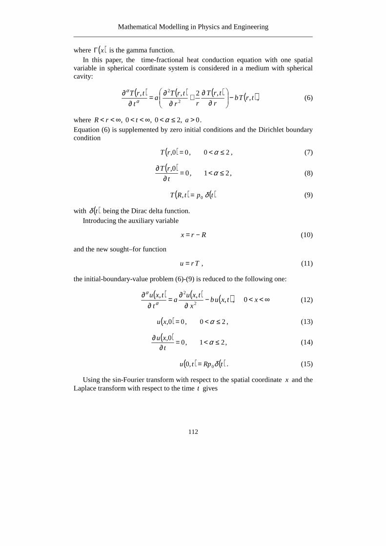
Mathematical Modelling in Physics and Engineering
112
where ( )xΓ is the gamma function. In this paper, the time-fractional heat conduction equation with one spatial
variable in spherical coordinate system is considered in a medium with spherical cavity:
( ) ( ) ( ) ( )trTb
r
trT
rr
trTa
t
trT,
,2,,2
2
−
∂∂+
∂∂=
∂∂
α
α, (6)
where .0,20,0, >≤<∞<<∞<< atrR α Equation (6) is supplemented by zero initial conditions and the Dirichlet boundary condition
( ) 20,00, ≤<= αrT , (7)
( ),21,0
0, ≤<=∂
∂ αt
rT (8)
( ) ( )tptRT δ0, = (9)
with ( )tδ being the Dirac delta function. Introducing the auxiliary variable
Rrx −= (10)
and the new sought–for function
Tru = , (11)
the initial-boundary-value problem (6)-(9) is reduced to the following one:
( ) ( ) ( ) ∞<<−∂
∂=∂
∂xtxub
x
txua
t
txu0,,
,,2
2
α
α (12)
( ) 20,00, ≤<= αxu , (13)
( ),21,0
0, ≤<=∂
∂ αt
xu (14)
( ) ( )tRptu δ0,0 = . (15)
Using the sin-Fourier transform with respect to the spatial coordinate x and the Laplace transform with respect to the time t gives
Mathematical Modelling in Physics and Engineering
113
( )bas
pRasu
++=
2
0* ,~ξ
ξξ α . (16)
Inversion of the integral transforms results in the solution
( ) ( )[ ] ( ) ξξξξπ
ααα
α dsin2
,0
2,
10 xtbaEtRpa
txu ∫∞
− +−= , (17)
where ( )zE βα , is the Mittag – Leffler function in two parameters βα , [5-7]
( ) ( ) Czn
zzE
n
n
∈>>+Γ
=∑∞
=,0,0,
0, βα
βαβα . (18)
Returning to the quantity ( )trT , according to (9), we get
( ) ( )[ ] ( )[ ] ξξξξπ
ααα
α dsin2
,0
2,
10 RrtbaEtr
RpatrT −+−= ∫
∞− . (19)
The results of numerical calculations are shown in Figs. 1-2. In calculations we have used the nondimensional quantities
Tp
tTbtb
R
taR
R
rr
0
2/
,,,, ===== αα
κξξ . (20)
When 0=b , the solution (19) coincides with the corresponding solution to the time-fractional diffusion-wave equation [4, 8].
Fig. 1. The fundamental solution to the Dirichlet problem for 0,5, 0,25α κ= = .
b 0
b 1
b 2
b 3
1.5 2.0 2.5 3.0 3.5 4.0r
0.02
0.04
0.06
0.08
T

Mathematical Modelling in Physics and Engineering
114
Fig. 2. The fundamental solution to the Dirichlet problem for 0 1,5α≤ ≤ ( 0,5, 0,25b κ= = ).
Keywords: heat conduction equation, Caputo fractional derivative, Laplace integral transform, sin-Fourier transform, Mittag – Leffler function
References
[1] Povstenko Y., Fractional heat conduction equation and associated thermal stresses, J. Thermal Stresses 2005, 28, 83-102.
[2] Povstenko Y., Thermoelasticity which uses fractional heat conduction equation, J. Math. Sci. 2009, 162, 296-305.
[3] Povstenko Y., Non-axisymmetric solutions to time-fractional diffusion-wave equation in an infinite cylinder, Fract. Calc. Appl. Anal. 2011, 14, 418-435.
[4] Povstenko Y., Linear Fractional Diffusion-Wave Equation for Scientists and Engineers, Birkhäuser, New York 2015.
[5] Gorenflo R., Mainardi F., Fractional calculus: integral and differential equations of fractional order. In: A. Carpinteri, F. Mainardi (Eds.), Fractals and Fractional Calculus in Continuum Mechanics, pp. 223-276, Springer, Wien 1997.
[6] Podlubny I., Fractional Differential Equations, Academic Press, San Diego 1999. [7] Kilbas A., Srivastava H., Trujillo J., Theory and Applications of Fractional Differential
Equations, Elsevier, Amsterdam 2006. [8] Povstenko Y., Fractional Heat Conduction Equation And Associated Thermal Stresses In An
Infinite Solid With Spherical Cavity, Quart. J. Mech. Appl. Math. 208, 61, 523-547.

Mathematical Modelling in Physics and Engineering
115
NUMERICAL ANALYSIS OF SANDWICH PANELS SUBJECTED TO TORSION
Zbigniew Pozorski
Institute of Structural Engineering, Poznan University of Technology, Poland [email protected]
The problem of torsion of sandwich panels with a shear deformable core is known in the literature. We can distinguish at least 3 theoretical approaches to this issue [1, 2, 3]. It is also worth noting that, in the analysis of torsion, it is important to distinguish the St. Venant torsion and the warping torsion. The problem of torsion was also analyzed experimentally and numerically, even in the papers [4, 5, 6].
In most typical cases, which concern the sandwich panels and take place in civil engineering, the effect of torsion is rightly ignored. Even if there are some load eccentricities, the torsion and the induced forces are very small (in practice negligible. For some time, with the tendency to enlarge the thickness of the core, this situation is changing. Even more drastic example, in which torsion is important, is the installation of an additional façade layer to the existing walls made of sandwich panels. The heavier and more distant the additional layer, the larger the torsion of the sandwich panel to which it is mounted.
In this paper, the influence of load and support boundary conditions on the internal forces and stresses in the sandwich structure subjected to torsion is mainly analyzed. The analyzes started with the schemes most close to the theoretically ideal conditions. Subsequently, the conditions to reflect the actual conditions were gradually sought. Although apparently the load and support boundary conditions of the wall panels seem to be fairly straightforward, in fact they are very difficult to reflect in a simple theoretical model. For this reason, it was decided to perform the appropriate numerical analysis.
The 3-D model consists of two thin steel facings and a thick but flexible core is considered in the paper. The sandwich structure is mounted to the steel substructure by means of mechanical fasteners. The easiest conditions imitating such a fixation were tried in the created models. A slightly different issue is a method of loading the sandwich panel. Various cases were considered, including concentrated force or load spreading in a certain area. The important question is whether, besides torsion, the applied load causes yet another force. The action of the force applied to the external facing induces additionally bending of the facing (in-plane) as well as shearing of the core resulting from the transmission of the load towards the supports. This transmission is one of the most interesting and, to date, poorly recognized phenomena. In-plane bending of the facings in also hides many unknowns. First of all, it is a question of uniformity of the load distribution on both facings. Second, there is some uncertainty about the proportions of the “sandwich

Mathematical Modelling in Physics and Engineering
116
beam” dimensions. A 3-D layered structure is often treated simply as a beam, although in the case in question it is closer to the slab structure. Finally, the effect of the local instability of thin facings should also be taken into account. So far, in engineering practice, the impact of in-plane bending of the facings (including the influence of this bending on local instability of facings) was simply neglected.
All of the above described aspects make the full interpretation of even the best performed numerical simulations very difficult. Despite this, this paper attempts to gradually organize the above described mechanical effects and parameters into the mechanics of layered structures, generated stresses and the safety of use of sandwich panels.
Keywords: sandwich panels, torsion, numerical simulations, finite element method, boundary conditions
References
[1] Stamm, K., Witte, H., Sandwichkonstruktionen. Springer Verlag, Wien, (in German) 1974. [2] Höglund, T., Load bearing strength of sandwich panel walls with window openings.
Proceedings of the IABSE Colloquium, Stockholm 1986, IABSE Report Vol. 49, 349-356. [3] Zenkert, D., The handbook of sandwich construction, EMAS Ltd., 1997. [4] Whitney, J.M., Analysis of anisotropic laminated plates subjected to torsional loading.
Composites Engineering 1993, 3 (6), 567–582. [5] Whitney, J.M., Kurtz, R.D., Analysis of orthotropic laminated plates subjected to torsional
loading. Composites Engineering 1993, 3 (1), 83–97. [6] Qiao, P., Xu, X.F., Refined analysis of torsion and in-plane shear of honeycomb sandwich
structures. Journal of Sandwich Structures & Materials 2005, 289 (7), 290–305.
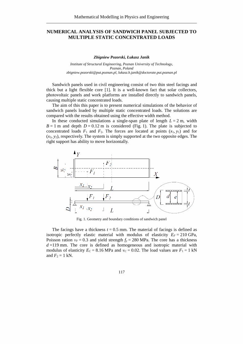
Mathematical Modelling in Physics and Engineering
117
NUMERICAL ANALYSIS OF SANDWICH PANEL SUBJECTED TO MULTIPLE STATIC CONCENTRATED LOADS
Zbigniew Pozorski, Łukasz Janik
Institute of Structural Engineering, Poznan University of Technology, Poznan, Poland
[email protected], [email protected]
Sandwich panels used in civil engineering consist of two thin steel facings and thick but a light flexible core [1]. It is a well-known fact that solar collectors, photovoltaic panels and work platforms are installed directly to sandwich panels, causing multiple static concentrated loads.
The aim of this this paper is to present numerical simulations of the behavior of sandwich panels loaded by multiple static concentrated loads. The solutions are compared with the results obtained using the effective width method.
In these conducted simulations a single-span plate of length L = 2 m, width B = 1 m and depth D = 0.12 m is considered (Fig. 1). The plate is subjected to concentrated loads F1 and F2. The forces are located at points (x1, y1) and for (x2, y2), respectively. The system is simply supported at the two opposite edges. The right support has ability to move horizontally.
Fig. 1. Geometry and boundary conditions of sandwich panel
The facings have a thickness t = 0.5 mm. The material of facings is defined as isotropic perfectly elastic material with modulus of elasticity EF = 210 GPa, Poisson ration νF = 0.3 and yield strength fy = 280 MPa. The core has a thickness d =119 mm. The core is defined as homogeneous and isotropic material with modulus of elasticity EC = 8.16 MPa and νC = 0.02. The load values are F1 = 1 kN and F2 = 1 kN.

Mathematical Modelling in Physics and Engineering
118
Numerical model was created as a 2D composite shell (three-layered shell). The model was discretized using four-node, conventional shell elements S4R, the mesh size was constant and equal to 0.10 m. This model was presented in [2]. The loads F1 = 1 kN and F2 = 1 kN were applied to single nodes.
The solutions obtained for numerical model were compared with the results obtained using the effective width method [3]. To get results from effective width method a superposition principle was used.
Comparing solution specified by EWD method and 2D numerical model, some discrepancies can be seen. To juxtapose it with work [4], it is observed that engineering EWD method is relatively safe but there are seem to be introduced some improvements in case of subjecting panels to multiple static loads. The obtained results encourage to conduct further analysis into the behaviour of sandwich panels subjected to multiple concentrated loads.
Keywords: sandwich panels, concentrated loads, numerical simulations, finite element method, the effective width method
References
[1] Davies J. M., (Ed.). Lightweight sandwich construction. John Wiley & Sons 2008. [2] Pozorski Z., Janik Ł., Analiza płyt warstwowych poddanych obciążeniom skupionym. W:
Budownictwo a środowisko : projektowanie i modernizacja obiektów budowlanych, red. Bromberek Z., Wydawnictwo Zarządu Oddziału PZITB w Poznaniu, Poznań 2017, 149-161 (in Polish).
[3] European Convention for Constructional Steelwork, European Recommendations for the Design of Sandwich Panels with Point or Line Loads, 2013.
[4] Pozorska J., Pozorski Z., Janik Ł., Numerical simulations of structural behavior of sandwich panels subjected to concentrated static loads. Journal of Applied Mathematics and Computational Mechanics 2017, 16(2), 113-121.

Mathematical Modelling in Physics and Engineering
119
ON A WEAK CONVERGENCE OF DENSITIES OF HOMOGENEOUS YOUNG MEASURES
Piotr Puchała
Institute of Mathematics, Czestochowa University of Technology, Czestochowa, Poland
Young measures appear in many engineering problems. In nonlinear elasticity, for example, we minimize the energy functional of the form
M = , M, ∇M \, (1)
where: - Ω is elastic body under consideration; - M is its displacement; it is usually an element of a suitable Sobolev
space ; - is the density of the internal energy.
The so called direct method is a widely used method of minimizing such functionals.
However, energy functionals of certain materials, as laminates or various types of alloys, do not attain their infima. It is connected with what engineers call ‘microstructure’ and is caused by the fact, that the density of the internal energy is not quasiconvex with respect to the third variable. The minimizing sequences M are functions of a highly oscillatory nature and are divergent in the strong topology of , but they are weakly∗convergent. It has been discovered by Laurence Chisholm Young in [4], that the weak* limits of the sequences of the form
, M, ∇M are in general not ‘common’ functions with domain of
definition being points in an appropriate space, but families of countably additive regular set functions. The members of these families are probability measures, nowadays called the Young measures. The existence of a Young measure associated with a measurable function (or with a sequence of oscillating functions) relies on the Riesz representation theorem. However, calculating an explicit form of a Young measure is in general a very difficult task.
The simplest form of a Young measure is a ‘homogeneous Young measure’. It is in fact a ‘one parameter family’, i.e. it does not depend on points of Ω. It serves as a source of examples and in many real world cases it is the generalized minimizer of the considered integral functional, see for example [1] and [4].
In [2] a relatively simple method of deriving an explicit form of a homogeneous Young measure is proposed. It avoids using complicated functional

Mathematical Modelling in Physics and Engineering
120
analytic machinery. Instead, a change of variable theorem for multiple integrals is used. The theoretical foundations making this method possible is described in detail in [4]. It turns out that following this approach it is relatively simply to characterize weak convergence of the densities of homogeneous Young measures. Moreover, this convergence appears to be equivalent to the weak convergence of the sequence of the Young measures under consideration, understood as elements of a Banach space of regular countable additive scalar measures (with a total variation norm). An application of the results to the Lebesgue-Stieltjes type integrals is also given.
Keywords: homogeneous Young measures, weak convergence of functions, weak convergence of measures
References
[1] Müller S., Variational models for microstructure and phase transitions, in Calculus of Variations and Geometric Evolution Problems, S. Hildebrandt and M. Struwe, editors, Lecture Notes in Mathematics, Vol. 1713, Springer Verlag, Berlin, Heidelberg, Germany, 1999, 85-210.
[2] Puchała P., An elementary method of calculating an explicit form of Young measures in some special cases, Optimization 2014, vol. 63 No.9, 1419-1430.
[3] Puchała, P., A simple characterization of homogeneous Young measures and weak convergence of their densities, Optimization 2017, vol. 66 No.2, 197-203.
[4] Roubíček T., Relaxation in Optimization Theory and Variational Calculus, Walter de Gruyter, Berlin, New York, 1997.
[5] Young L.C., Generalized curves and the existence of an attained absolute minimum in the calculus of variations, C. R. Soc. Sci. Lett. Varsovie, Classe III, 1937, 30, 212-234.

Mathematical Modelling in Physics and Engineering
121
FREE VIBRATION OF EULER-BERNOULLI BEAMS MADE OF AXIALLY FUNCTIONALLY GRADED MATERIALS
Jowita Rychlewska
Institute of Mathematics, Czestochowa University of Technology, Czestochowa, Poland
In the paper free vibration of axially functionally graded (FG) beams is analyzed within the framework of the Euler-Bernoulli beam theory. The proposed method relies on replacing functions characterizing FG beams by piecewise exponential functions. The analytical solution of the problem is used for numerical analysis. The effect of selected parameters characterized the system on the free vibration frequencies for different boundary conditions is investigated.
Functionally graded beams are composites characterized by the volume fraction of different materials which is varied continuously with the thickness and/or the length of the beam. Through an appropriate selection of the volume fraction the FG beam with expected thermal and mechanical properties can be obtained. Therefore, the FG beams can be used in various engineering applications.
The literature on vibration analysis for axially graded beams is very extensive. For example, Wu et al. [1] applied the semi-inverse method to find the solutions to the dynamic equation of axially functionally graded simply supported beams. Huang and Li [2] studied free vibration of axially functionally graded beams by using the Fredholm integral equations. Hein and Feklistova [3] applied the Haar wavelet approach to analyse free vibration of axially functionally graded beams. The differential transform element method and differential quadrature element method of lowest order were used to solve free vibration and stability problems of FG beams by Shahba and Rajasekaran [4]. The exact solution to free vibration of exponentially axially graded beams was presented by Li et al. [5]. Explicit frequency equations of free vibration of exponentially FG Timoshenko beams were derived by Tang et al. [6]. Huang et al. [7] presented a new approach for investigating the free vibration of axially functionally graded Timoshenko beams. By applying auxiliary functions they transformed the coupled governing equations into a single governing equation. Moreover, there are some studies related with the problem of free vibration of FG beams, where the gradation of material is assumed to be along any of the possible Cartesian coordinates, see Alshorbagy et al. [8], Shahba et al. [9]. A review of researches on FG beam type structures can be found in Chauhan and Khan [10].
In this contribution a new approach to free vibration analysis of FG beams with arbitrary axial inhomogeneity. The main idea presented here is to approximate FG beam by an equivalent beam with piecewise exponentially varying material and

Mathematical Modelling in Physics and Engineering
122
geometrical properties. The proposed method is a certain generalization of the approach presented in Kukla and Rychlewska [11].
Keywords: axially graded beam, free vibration, Euler-Bernoulli beam theory
References
[1] Wu L., Wang Q., Elishakoff I., Semi-inverse method for axially functionally graded beams with an anti-symmetric vibration mode, Journal of Sound and Vibration, 2005, 284, 1190-1202.
[2] Huang Y., Li X.-F., A new approach for free vibration of axially functionally graded beams with non-uniform cross-section, Journal of Sound and Vibration, 2010, 329, 2291-2303.
[3] Hein H., Feklistova L., Free vibrations of non-uniform and axially functionally graded beams using Haar wavelets, Engineering Structures, 2011, 33, 3696-3701.
[4] Shahba A., Rajasekaran S., Free vibration and stability of tapered Euler-Bernoulli beams made of axially functionally graded materials, Applied Mathematical Modelling, 2012, 36, 3094-3111.
[5] Li X.-F., Kang Y.-A., Wu J.-X., Exact frequency equations of free vibration of exponentially functionally graded beams, Applied Acoustics, 2013, 74, 413-420.
[6] Tang A.-Y., Wu J.-X., Li X.-F., Lee K.Y., Exact frequency equations of free vibration of exponentially non-uniform functionally graded Timoshenko beams, International Journal of Mechanical Sciences, 2014, 89, 1-11.
[7] Huang Y., Yang L.-E., Luo Q.-Z., Free vibration of axially functionally graded Timoshenko beams with non-uniform cross-section, Composites: Part B, 2013, 45, 1493-1498.
[8] Alshorbagy A.E., Eltaher M.A., Mahmoud F.F., Free vibration characteristics of a functionally graded beam by finite element method, Applied Mathematical Modelling, 2011, 35, 412-425.
[9] Shahba A., Attarnejad R., Zarrinzadeh H., Free vibration analysis of centrifugally stiffened tapered functionally graded beams, Mechanics of Advanced Materials and Structures, 2013, 20, 331-338.
[10] Chauhan P.K., Khan I.A., Review on analysis of functionally graded material beam type structure, International Journal of Advanced Mechanical Engineering, 2014, 4, 3, 299-306.
[11] Kukla S., Rychlewska J., Free vibration of axially functionally graded Euler-Bernoulli beams, Journal of Applied Mathematics and Computational Mechanics, 2014, 13, 1, 39-44.

Mathematical Modelling in Physics and Engineering
123
MULTI-LAYER NEURAL NETWORKS FOR SALES FORECASTING
Magdalena Scherer
Department of engineering management, Czestochowa University of Technology, Czestochowa, Poland [email protected]
Forecasting and the ability to assess future events play a key role in business operations. The uncertainty of the future and the time interval from the moment of the decision to its result, makes it necessary to find appropriate prognostic methods, which are burdened with the smallest error and are simple and inexpensive to use. With accurate and accurate forecasting, decision making becomes much easier, making enterprise management easier. Forecasts should be the basis for creating business action plans. Still, new methods of forecasting are being sought, where the results will be as small as possible, and the methods will be simple and cheap to use.
Neural networks are mathematical structures and their software or hardware models. The inspiration for their construction was the natural neurons connected by synapses and the entire nervous system, and in particular its central point – the brain. Artificial neural networks can be used in a broad spectrum of data processing issues, such as pattern classification, prediction, denoising, compression and image and sound recognition, or automation.
Neural networks have the ability to process incomplete data and to provide approximate results. They enable fast and efficient processing of large amounts of data. They are resistant to errors and damage.
Fig. 1. Artificial neuron model

Mathematical Modelling in Physics and Engineering
124
The basic element of the neural network is the neuron [4]. Figure 1 shows the neuron model, where > is the number of inputs to the neuron, , … , are input signals, N, … , N are synaptic weights, is the output value, N is bias and is activation function. The operation of the neuron can be described using the formula
= <, (1) where < = ∑ ##& N# (2)
The input signals , … , are multiplied by the corresponding weights N, … , N. The resulting values are summed to produce a signal s. The signal is then subjected to an activation function that is usually nonlinear to create many layers. There are many models of neural networks. The neural network division can be made taking into account the following factors: learning method, direction of signal propagation in the network, type of activation function, type of input data and method of interconnection between neurons.
Neural networks consist of interconnected neurons. Depending on how these connections are made, three types of neural networks are distinguished: feedforward, feedback networks, convolutional and cellular networks. In feedforward, one-way networks, the flow of signals is always in one direction, from the input to the output. Neuron outputs from one layer are neuron inputs in the next layer. On feedback networks, also known as recursive, some of the output signals are simultaneously input signals. In networks of this type, the activation of the network by the input signal causes the activation of some or all of the neurons in the, so-called, network relaxation process. Therefore, in order to validate the operation of the network, a stability condition should be added. The stimulated network must reach a stable state where the baseline values of the neurons remain constant, this process should take place at finite time. On the other hand, in cellular neural networks, each neuron is connected to neighboring neurons.
Most commonly used neural architecture, both in research and commercial models, are perceptron networks. These are unidirectional networks where neurons are grouped in at least two layers. The first layer is called the input layer and the last layer is the output layer. There may be one or more hidden layers between these layers. Signals are passed from the input layer to the output layer, without feedback to the previous layers. The diagram of the three-layer neural network is shown in Figure 2, where , … , denote input signals and , … , as output signals.
The number of neurons in each layer is important in the operation of the network. Too many neurons increase the learning process. In addition, if the number of learning samples in relation to network size is small, the network can be "learned" and thus lose the ability to generalize knowledge. In this case, the network will learn the learning sequence "by heart" and will probably only correctly map the samples that were included in it. Therefore, after learning the network, we should check the correctness of its operation. For this purpose, a test dataset consisting of samples that were not present in the network learning process
Mathematical Modelling in Physics and Engineering
125
is used. Only after testing it is possible to tell whether the network has been properly trained and is working properly.
There are two methods of learning neural networks: supervised learning and unsupervised learning. Network learning involves enforcing a specific neural network response to the input signals. That is why a very important moment in research is the right choice of learning method. Supervised teaching, also called learning with a teacher, involves modifying weights so that the output signals are as close as possible to the desired values. Training data includes both input signal groups and desired values for responding to these signals. A special case of supervised learning is reinforcement learning, where the network is trained not to give exact values of the desired output signals, only the information or whether it responds correctly. Unattended learning, called non-teacher learning, is a self-parsing study of dependence in a test set by a neural network. During learning, the network receives no information about the desired response. Training data contains only a set of input signals. Networks with such action are called self-organizing or self-associative.
Neural networks can, on the basis of data, learn a broad spectrum of problems. They are better than traditional computer architectures in tasks that people perform naturally, such as image recognition or generalization of knowledge. Advances in computer technology and network learning algorithms have resulted in a steady increase in the complexity of tasks solved by neural networks. New architectures are also emerging, such as convolutional neural networks being able to classify hundreds of image classes.
Neural networks are used to solve different problems [2][3]. However, every problem requires a proper network adaptation. An appropriate network topology, the number of neurons in layers, and the number of network layers must be selected. Next, we need to prepare a training and testing set. The network must be trained learn first and then the correct operation of the network must be verified.
This paper concerns forecasting sales volume in monthly intervals in a medium Polish company. The data from previous months were used to train feedforward neural network (full-connected) with the backpropagation algorithm [1]. We achieved a good prediction accuracy what allows to use the outcome to increase the effectiveness of the company management.
Keywords: data forecasting, machine learning, artificial neural networks
References
[1] Rumelhart, David E.; Hinton, Geoffrey E.; Williams, Ronald J. (8 October 1986). Learning representations by back-propagating errors, Nature. 323 (6088): 533–536.
[2] Ke Y., Hagiwara M., An English Neural Network that Learns Texts, Finds Hidden Knowledge, and Answers Questions, Journal of Artificial Intelligence and Soft Computing Research, Volume 7, Issue 4, pp. 229-242.

Mathematical Modelling in Physics and Engineering
126
[3] Bologna G., Hayashi Y., Characterization of Symbolic Rules Embedded in Deep DIMLP Networks: a Challenge to Transparency of Deep Learning, Journal of Artificial Intelligence and Soft Computing Research, Volume 7, Issue 4, pp. 265-286.
[4] Bishop, Christopher M. Neural networks for pattern recognition. Oxford university press, 1995.

Mathematical Modelling in Physics and Engineering
127
FEATURE EXTRACTION OF FOREARM-VEIN PATTERNS BASED ON REPEATED LINE TRACKING
Dorota Smorawa , Mariusz Kubanek
Institute of Computer and Information Sciences, Czestochowa University of Technology, Czestochowa, Poland
[email protected], [email protected]
A biometrics system for identifying individuals using the pattern of veins in a forearm was proposed. The system has the advantage of being resistant to forgery because the pattern is inside a forearm. Infrared light is used to capture an image of a forearm that shows the vein patterns, which have various widths and brightness that change temporally as a result of fluctuations in the amount of blood in the vein, depending on temperature, physical conditions, etc. The proposed method extracts the finger-vein pattern from the unclear image by using line tracking that starts from various positions. The proposed method extracts the forearm-vein pattern from the unclear image by using line tracking that starts from various positions. The algorithm described is a component of the whole system, which is based on the pattern of the veins of the palm and forearm.
Image processing techniques can be used to enhance blood vein portion of captured image of the forearm. Image enhancement is one among the most widely researched area of digital image processing. The primary purpose is to produce image of better quality and interpretability from the original image. Various techniques in image processing have been widely used in divergent applications, such as biomedical, biometrics and many others. There are different approaches introduced for blood vein identification and enhancement. In work [1] they proposed a method for real-time blood vein enhancement by capturing an infrared image of blood vein. But a costly camera and processing equipment are used to capture and process vein images. In work [2], authors used background reduction filter for vein contrast enhancement of finger vein patterns captured in near-infrared regions for personal identification. A Method for Hand Vein Recognition Based on Curvelet Transform Phase Feature used Curvelet transform of the region of interest and encoded the Curvelet coefficients phase variance, and evaluate the Chi-square distance of coding histogram for vein recognition [3]. Image Restoration and Enhancement for Finger-Vein Recognition by authors of work [4] followed image processing by using Gabor filters. In above cases they took images using transmitted IR rays by placing IR sources below hand and took images of top part of hand. The literature [5], discusses hand vein pattern recognition using an image descriptor for biometric applications. For the biometric application, only the statistical structure of the vein is required, rather than the exact contours of the vein. In most of the studies, blood vein pattern of fingers or palm is extracted as an alternative to fingerprints used in biometry [6-11]. In such cases the exact structure

Mathematical Modelling in Physics and Engineering
128
need not be extracted as only the pattern is necessary for biometric applications. Apart from this, infra-red imaging commonly utilises transmitted infra-red images which has a higher visibility of veins. Hence, better results can be obtained from simple thresholding and normal enhancement techniques. In antecubital fossa, taking transmitted IR images are not possible. Hence reflected near infrared images, which has very low visibility of veins, are used in this research. The proposed algorithm follows a different approach for blood vein identification and enhancement efficiently. The method is mainly based on analysis of contrast and thresholding.
In this paper, an efficient method for enhancement of blood vein on the forearm is devised with the help of contrast limited adaptive histogram equalisation. The image captured in near-infrared region is converted into grey scale and made to undergo to achieve an amplification limited contrast enhancement [12] of all the objects in the image. The blood vein is extracted from the image using thresholding method. Erosion is performed for better accuracy of vein segments identified, and region of interest (ROI) is identified to increase the efficiency of the blood-vein detection.
Infrared image acquisition of forearm
NIR image acquisition is done with the help of a modified digital camera. The modification is done in by replacing IR filter of the camera placed in front of charge coupled device with a visible light filter. IR flash is used for uniform illumination of hand and took images with the help of reflected IR signals from the forearm. The image stored in JPEG format is shown in Figure 1.
Fig. 1. Image captured using modified camera
This captured image is processed for blood vein enhancement. Initially, the image was pre-processed and then converted RGB image to greyscale. The intensity level is expressed within the range 0 to 255 in the case of 8-bit image. The blood vein part in forearm image is not distinctly visible compared to body skin part. For vein image enhancement and extraction it is needed to distinguish blood vein from other skin. Histogram equalization process will help to enhance the contrast of each object in particular images separately. This process will stretch out intensity ranges [12]. It is done by mapping of intensity distribution (given histogram) to another distribution with a wide range of intensity values. Blood-vein

Mathematical Modelling in Physics and Engineering
129
images, which are low contrast dark locales, global histogram equalization, won't work viable. Even if the forearm blood vein images are enhanced by using adaptive histogram equalization, vein edges are might not be properly visible in most of the cases. Additional imaging techniques are needed to extract the shape of the veins. Binarization and morphological denoising create a clearer picture of the veins. For proper extraction of blood veins from the surrounding skin, selection of threshold levels is crucial. Thresholding algorithm helps for finding suitable threshold level that efficiently extracts blood veins from the image. This algorithm performs image thresholding based on clustering [13]. By assuming the image consists of two classes of pixels, this algorithm calculates an optimal threshold value to separate the classes such that their intra-class variance is minimum and inter-class variance is maximum. Figure 2 shows the original loaded image. The binary image is shown in Figure 3.
Fig. 2. Loaded original image
Fig. 3. Image after binarization
Morphological operations have included closure operations and the removal of minor disturbances. It is needed to perform morphological operations on the vein part extracted to get a more precise shape of the vein. Dilation and Erosion are mainly carried out in the post-processing for this purpose. Dilation adds pixels to the boundaries of objects in an image, while erosion removes pixels on object boundaries. Here erosion is performed, as the operation helps to remove the

Mathematical Modelling in Physics and Engineering
130
unwanted sections which may get extracted with the vein. The result of the morphological transformations is shown in Figure 4.
Fig. 4. Image after morphological transformations
The captured images for processing may contain portions other than forearm part which is not the region of interest. To find region of interest (ROI), the captured image is thresholded with a median pixel value around 100. This is the separating pixel value between skin and background surface. The portion of the skin where the vein is present is needed to be processed. Hence, surface part is discarded, and the region of interest is extracted.
Lines are determined by the yellow-green or blue-red markers. Different colors represent different directions of veins. The result of this operation is shown in Figure 5.
Fig. 5. Designated veins, marked by colorful crosses
The next operation involves removing lines for which the number of markers in one string is too small. Such processing leaves only the main vein patterns that have the greatest impact on the quality of recognition. The image after removing the small lines is shown in Figure 6.

Mathematical Modelling in Physics and Engineering
131
Fig. 6. Final processing effect
Forearm blood vein identification is quite difficult. This proposed algorithm extracted and enhanced blood vein from forearm hence providing more visibility apart from skin. The algorithm tested infrared forearm images and result shows the efficiency of this algorithm. It is an element of the entire system that uses the palm vein and forearm to identify and verify users.
Keywords: user identification, user verification, palm vein forearm vein
References
[1] Zeman H.D., Lovhoiden G., Vrancken C.. The Clinical Evaluation of Vein Contrast Enhancement. Proc of the 26th annual international conference of IEEE EMBS, San Francisco, CA, USA, 2004.
[2] Kono M., Ueki H., Umemura S.I., Near-infrared finger vein patterns for personal identification. Appl Optics 2002, 41, 7429-7436.
[3] Shangqing W., Gu X., A method for hand vein recognition based on curvelet transform phase feature. Transport, Mechanical, and Electrical Engineering (TMEE), 2011 International Conference on IEEE, 2011.
[4] Yihua S., Yang J., Image restoration and enhancement for finger-vein recognition. IEEE 11th International Conference on Signal Processing (ICSP), 2012.
[5] Premalatha K., Natarajan A.M., Hand Vein Pattern Recognition using Natural Image Statistics. Defence Scientific Journal, 2015, 65, 150.
[6] Wang J., Wang G., Li M., Du W., Hand vein recognition based on PCET. Optik – International Journal Light Electron Optics 2016, 127, 7663-7669.
[7] Lingyu W., Leedham G., A thermal hand vein pattern verification system. International Conference on Pattern Recognition and Image Analysis, Springer, Berlin, Heidelberg, 2005.
[8] Qiu S., Liu Y., Zhou Y., Huang J., Nie Y., Finger-vein recognition based on dual-sliding window localization and pseudo-elliptical transformer. Expert Systems Application 2016, 64, 618-632.
[9] Smorawa D., Kubanek M., Biometric Systems Based of Palm Vein Patterns. Journal of Telecommunications and Information Technology, 2015, 2, 18-22.

Mathematical Modelling in Physics and Engineering
132
[10] Kubanek M., Smorawa D., Verification of Identity Based on Palm Vein and Palm-Print. Advances in Intelligent Systems and Computing, Soft Computing in Computer and Information Science, 2015, 342, 139-146.
[11] Kubanek M., Smorawa D., Holotyak T., Feature Extraction of Palm Vein Pattern Based on Two-Dimensional Density Function. Lecture Notes in Artificial Intelligence, Part II, 2015, 9120, 101-111.
[12] Smorawa D., Kubanek M., Comparison of Global Methods for the Image Contrast Enhancement Based on Biometric Images. Journal of Applied Mathematics and Computational Mechanics, 2016, 15(2), 137-146.
[13] Mehmet S., Survey over image thresholding techniques and quantitative performance evaluation. J Electronic Imaging, 2004, 13, 146-168.

Mathematical Modelling in Physics and Engineering
133
AN INFLUENCE OF THE PARAMETERS OF LOADING HEADS ON THE LOADING CAPACITY OF A DAMAGED COLUMN
SUBJECTED TO A SPECIFIC LOAD
Krzysztof Sokół
Institute of Mechanics and Machine Design Foundation, Czestochowa University of Technology, Czestochowa, Poland [email protected]
The studies on an influence of the parameters of the loading heads on the loading capacity of the cracked column subjected the specific load realized by the circular elements of heads are presented in this paper. The crack is simulated by means of the rotational spring. The boundary problem is formulated with the use of the minimum total potential energy principle on the basis of which the differential equations as well as natural boundary conditions are obtained. The main scope of investigations is to estimate whereas it is possible to increase the loading capacity of the cracked system by means of proper selection of the parameters of the loading heads.
In the figure 1 the investigated system is presented. The external load is realized by means of the loading heads with circular outline. The presence of the crack divides a column into two elements. During numerical calculations the crack is always opened and is simulated by the rotational spring of C stiffness which is calculated with consideration of [1]. The continuity of transversal and longitudinal displacements as well as bending moments and deflection angles is satisfied by natural boundary conditions in the point of crack presence. The total length of the structure is l=l1+l2. The loading head of radius R can move smoothly in the vertical direction. The radius R has a center in the point localized below the loaded end of the column on its undeformed axis through which passes the line of P force action (pole point). The radius of the receiving head is r and the distance between the end of the column and the contact point of both heads is l0. The adequate combination of the parameters of the loading heads may lead to the systems subjected to Euler’s load – comp. [2].

Mathematical Modelling in Physics and Engineering
134
W2(x2,t)
C
P
Rod (1) E, ρ, J1, A1
l2
W1(x1,t)
x2
x1 l1
Rod (2) E, ρ, J2, A2
Loading head
Receiving head
Loading head
R
r
Column’s top end
lk
Receiving head
l0 = lk+r
Fig. 1 The investigated column and shapes of heads
Keywords: computational mechanics, stability, crack, loading capacity
References
[1] Ostachowicz W.M., Krawczuk M., Analysis of the effect of cracks o the natural frequencies of cantilever beam, Journal of Sound and Vibration, 1991, 150(2),191–201.
[2] Tomski L. Uzny S., Vibrations and stability of a column subjected to the specific load realized by circular elements of heads, Mechanics and Mechanical Engineering, 2013, 17(2) ,197–206.
Mathematical Modelling in Physics and Engineering
135
REMARKS ON THE IMPACT OF THE ADOPTED SCALE ON QUALITY OF PRIORITY ESTIMATION
Tomasz Starczewski
Institute of Mathematics, Czestochowa University of Technology, Czestochowa, Poland
Analytic Hierarchy Process (AHP) is the method which supports people decisions, which consists on the best choice from the possible alternatives. In the AHP the decision maker (DM) answers the question in order to comparing every two among all possible alternatives in respect to any criterion. In this way the pairwise comparison matrix (PCM) arises. In this matrix, element in i-th raw and j-th column says how much more (or less) DM prefer i-th over j-th alternative [1].
PCM consists of numbers which correspond to DM answers about his judgment of preference. However DM answers are expressed in "linguistic values" not directly in numerical values. So we need convert the answers in common language to numbers. For this purpose priority scales are used. T. Saaty introduce such a scale, called Fundamental Scale (FS) [1], which consists of 9 natural numbers and its reciprocals which are connected with certain linguistic expressions:
FS = ¢ ,
£ , ¤ ,
¥ , ¦ ,
§ , ¨ ,
, 1, 2, 3, 4, 5, 6, 7, 8, 9 (1)
Despite of some negative opinions of using FS [2],[3], it is the most popular scale in AHP practice.
Apart of FS we investigate any other scale. The extension of FS to the set of 50 natural numbers scale is called in our presentation Extension Scale ES50:
ES50 = ³ ¦ ,
§¢ , §£ , ⋯ ,
¨ , , 1, 2, 3, … , 49, 50´ (2)
The ES50 is similar to the FS but allows comparing more different alternatives without dividing alternatives on classes (idea of Saaty [1]).
A little less popular than FS but also often encountered in literature is the Geometric Scale (GS) [4]. In difference to the previous scales, GS consists of numbers which create geometric sequence. We adopted GS1.2,10, it is GS consists of 10 succeeding natural powers of 1.2 and theirs reciprocals:
GS1.2, 10 = 1.2%, … , 1.2 (3)
The numbers in GS, in difference to FS, can be interpreted as actual ratios between related linguistic expressions.

Mathematical Modelling in Physics and Engineering
136
Interesting case for us is without rounded to scale PCM. Obviously, this case is not observed in practice but it help us to find out more information about impact of assumed scales on the final decisions quality.
In common AHP practice DM compares every pair of alternatives with respect to any criterion only one time (if you would compared A to B you do not have to compare B to A). It seems quite logical that reliable DMs to the same extent prefer alternative A to B as do not prefer B to A. However in practice when DMs compare A to B and B to A, they often give no reciprocal answers so in our paper we consider both cases: reciprocal and no reciprocal matrices [2],[4],[6].
The purpose of AHP is ordering the alternatives. In order to that the vector of numbers which indicates relative importance of alternatives is calculated. Such a vector which consists of indicating importance numbers we called priority vector (PV). We use in our research the Raw Geometric Mean Procedure to obtain PV from PCM [8].
The issue which we investigate is impact of the adopted scales for quality of decision in AHP. The natural indicators of scale properties are values of errors appearing in PVE when we use particular scales. For calculate values of relative errors in PV and frequency of appearing errors in ordering PV we run Monte Carlo experiments, which are based on A. Grzybowski experiments [2]. We observe an explicit impact of the adopted scales and PCM reciprocity to amount of errors in PV. When we look at obtained in our experiments results, it seems obvious, that adopted certain scales give better results with less amount of errors than the other.
Keywords: Analytic Hierarchy Process, Priority Scales, Pairwise Comparison
References
[1] Saaty T., Decision making – the analytic hierarchy and network processes (AHP/ANP), Journal Of Systems Science And Systems Engineering, Vol. 13, No. 1, pp1-35, March, 2004
[2] Grzybowski A.Z., New results on inconsistency indices and their relationship with the quality of priority vector estimation, Expert Systems With Applications 43 (2016) 197–212
[3] Franek J., Kresta A., Judgment Scales and Consistency Measure in AHP, Procedia Economics and Finance 12 (2014) 164 – 173
[4] Lootsma, F., Conflict Resolution via Pairwise Comparison of Concessions. European Journal of Operational Research. Elsevier, Amsterdam, 1989, 40(1), 109–116
[5] Dijkstra T. K., On the extraction of weights from pairwise comparison matrices, Central European Journal of Operations Research, January 2013, Volume 21, Issue 1, pp 103–123
[6] Crawford G., Williams C.A., A note on the analysis of subjective judgment matrices, Journal of Mathematical Psychology, 1985, 29, 387–405.
[7] Grzybowski, A. Z. Note on a new optimization based approach for estimating priority weights and related consistency index. Expert Systems with Applications, 39 (2012) 11699–11708.

Mathematical Modelling in Physics and Engineering
137
LEARNING TOOLS IN COURSE ON SEMANTICS OF PRORGAMMING LANGUAGES
William Steingartner, Valerie Novitzká
Faculty of Electrical Engineering and Informatics, Technical University of Košice, Košice, Slovakia
[email protected], [email protected]
Abstract. Formal methods are intended to systematize and introduce rigor into all the phases of software development. The semantics of programming languages is important for software engineers and IT experts to understand the meaning of programs and/or behaviour of them. The programming language used for software development furnishes precise syntax and semantics for the implementation phase. Based on our experience with teaching formal semantics of programming languages we have prepared a packet of modules, that helps us and to students to understand the most popular semantic method - structural operational semantics. The first module translates a program written in a programming language to abstract machine code, the second module makes reverse translation from code to program source text and the third one emulates stepwise execution of abstract machine code. Our packet can be easily extended for other semantic methods.
1. Introduction
Software engineering is a young engineering discipline that is different in many respects from the classical engineering fields. One of preconditions for efficient implementation of software development methods is understanding the formalism without which these methods could not be developed [1]. On the present the computer science increases making use of formal models to help the understanding of complex software systems and to reason about their behaviour, in particular to verify the correctness of the system (or at least some desired aspects of its behaviour) with respect to a formal specification. Then more and more tools support software development on the basis of formal methods. All of these tools and techniques are well grounded in formal models of system execution which are rooted in the formal semantics of the underlying programming languages. The term formal methods pertains to a broad collection of formalisms and abstractions intended to support a comparable level of precision for other phases of software development. While this includes issues currently under active development, several methodologies have reached a level of maturity that can be of benefit to practitioners. The necessity of formal methods education has developed from its increasing assimilation into systems development within industry [2]. By providing precise and unambiguous description mechanisms, formal methods facilitate the understanding required to coalesce the various phases of software development into a successful endeavour. To help future generations of software developers and

Mathematical Modelling in Physics and Engineering
138
engineers profit from these exciting developments, however, it is necessary to adequately educate and train them in the basics of formal logic and formal language semantics.
Semantics is an integral part of formal definition of a programming language. Semantics provides a meaning of a program and can help during its design and implementation. Now several semantic methods are known, e.g. denotational semantics, operational semantics, action semantics, axiomatic semantics, categorical semantics and others. In this paper we concern with software which could help to understand an operational semantics, a very popular semantic method which provides meaning of the execution steps of a program and it is better understandable for those who are not familiar with mathematics.
Operational semantics was introduced by Gordon Plotkin in [3]. It is widely used also by practical programmers. This method defines a meaning of every step of program execution by transition relations between states before and after a given statement execution. In contrast with other semantic methods we have quite positive experience in teaching this method, because it is understandable for students and software engineers as it requires minimal knowledge of mathematics. Operational semantics incorporates abstract implementation on an abstract machine that enables partial verification of programs [4]. An important tool for explanation this method and for easy understanding by students seems to be a packet of programs illustrating translation from program text to the code of abstract machine and vice versa together with step by step execution.
The aim of our paper follows from the ideas mentioned above. We present our packet consisting of three modules. Each of modules behaves as separated program and can be run independently. The first one translates a program text written in the simple language Jane to a code (sequence of instructions) of abstract machine, the second one performs the reverse process, i.e. it provides a program text in Jane from a code of abstract machine and the third one is an emulator of the stepwise execution of a code on abstract machine. These three programs afforce in significant measure the appreciation of this method by students and help them to achieve skills in defining operational semantics of programming languages.
Sections 2, 3 and 4 concern with the design and implementation of three programs: from program text to code, from code to program text and the stepwise execution of AM code. This integrated packet has intermediate output that is intended to the extension for other semantic methods.
2. Compiler from Jane to AM code
We briefly describe in this section the specification and implementation of the first module - a compiler from language Jane to Abstract Machine (AM) code and algorithms of its primary and secondary functions.
This program is designed as an application, that provides the translation of a program written in Jane language into the code of AM.
An input is a source text, that represents a program in Jane. We do not consider variables' declarations here, so the program consists only of a body. An output is
Mathematical Modelling in Physics and Engineering
139
a final code which is either a sequence of AM instructions or XML form. The machine comprises only a program store.
The module consists of the standard compiler phases according to [5]. The main function of lexical analysis in this application is tokenization, i.e. dividing the program into valid tokens, elimination of all unnecessary white characters and checking of the number of brackets. In the syntax analysis we use the top-down parsing method with error recovery which consists of a set of recursive procedures that gradually examine the syntax in more and more detail. A recursive descent parser contains a possibly recursive procedure for each syntactic construct. Then each statement is checked if it matches the appropriate regular expressions. For each statement of Jane language an unique regular expression is defined. If the cycle statement (while-do) or conditional statement (if-then-else) are found, they are matched recursively with appropriate regular expressions. After the syntax analysis, a very simple semantic analysis is performed: the type mismatch control in assignments and Boolean conditions in statement constructs.
The compiler is able to generate two kinds of output, based on a user's choice. The first kind of output is a sequence of instructions in AM code. This function of compiler is the default one. The AM instructions are generated according to the translation rules (listed in [6]). The second kind of output is an XML document developed for future extension of the teaching software. It could allow to take an XML form of an input program and to use it as an input for the other semantic methods, e.g. a construction of the derivation trees in natural semantics [7] or a graphical representation of program in categorical semantics [8] etc.
The module consists of the classes. The main class GenerateJPJtoAM_UI provides communication and interaction with user. The class InputTokenizer represents a lexical analysis. The class RegexPatterns is used in syntax analysis and it provides the regular expressions for matching the keywords of the Jane language and expressions. Class Generator is used as generator of instructions. Particular classes for generating the instructions for each statement are derived from the main generator class. These classes define the following translation rules:
• class StoreGenerator - for the assignment; • class SkipGenerator - for the empty statement;
• class IfGenerator - for the conditional statement;
• class WhileGenerator - for the logical prefix cycle; • class BooleanGenerator - for the Boolean expressions.
The class XmlGenerator is used for generating the XML format of a source program. The general class diagram is depicted in Fig. 1.

Mathematical Modelling in Physics and Engineering
140
Fig. 1 Class diagram
3. Reverse compilation from AM code to Jane
The second module is a decompiler from AM code into Jane source. This program allows to reconstruct code in Jane when a sequence of instructions in AM code is given. Decompilation is the reverse process of compilation i.e. creating higher level language code from machine/assembly language code used mainly in refactoring. At the basic level, it just requires to understand the machine/assembly code and rewrite it into a high level language. Although there are many questions about ethics of decompilation, we use in education simple decompilation from AM code to Jane only for teaching purposes.
The program loads an input and starts with splitting the input sequence into particular instructions storing them in a data structure list. The compound instructions BRANCH and LOOP are considered also as separate instructions together with their contents, where other recursive splitting to the sequences of instructions are applied and new instruction lists are built up.
The next step is recognizing the instructions in the list and reconstructing the Jane code. Each instruction is matched with patterns. If an instruction representing an arithmetic or Boolean operation or instruction representing a value is found, an appropriate symbol or a value is stored in a stack until the end of expression is being reached. The correct ending of any well-formed expression is either the instruction STORE (assignment statement), or the instruction BRANCH (conditional statement), or the empty string (LOOP instruction). At the end the expression is built up from the stack.
If the expression is ended by the instruction STORE, then the arithmetic expression is constructed from stack as right-hand side of the statement, after that the content of the stack is released. If the expression is ended by the instruction
Mathematical Modelling in Physics and Engineering
141
BRANCH, then Boolean expression is constructed from the stack and included into if-then construction, then two other recursive instruction parsing runs are executed: the first one for then-branch, the second one for the else-branch. If the instruction LOOP is found, then also two other recursive code constructions are executed: the first for the Boolean expression, the second one for the body of cycle. Then both strings are included into while-do construction. If the instruction EMPTYOP is found, an empty statement skip is provided as the output. Finally, when the code reconstruction is finished with success, the code in Jane can be stored in a text file.
4. Emulator of AM
The last module in our packet is an emulator of AM code. The program is implemented in Java programming language, too.
The program loads an input code in the form of AM instructions. By their processing and splitting into several steps, the output is produced by illustrating the changes performed in an expression stack and states after execution of particular instructions.
At the beginning, an input sequence of instructions is read from the file or is typed manually. After that, the code is analysed by matching the patterns of instructions. The sequence is split into separate instructions. Compound instructions BRANCH and LOOP are considered as separate instructions together with the other sequences of instructions. During this analysis all variables in an input source are found and written into table of variables. In this phase, if a syntax error is found, the user is notified about the problematic part of the code. If the syntax checking is completed without errors, then variables can be initialized by user and the analysed AM source is ready to be executed.
The execution of code provides a complete code processing respecting the semantics of instructions listed in [6]. During the stepwise execution the new states on a stack and in memory state are computed. The program displays an actual AM configuration before and after the execution of an actual instruction.
Although the program is syntactically correct, it can contain unknown (hidden) fault [9]. For example, during the program execution an infinite cycle can occur. The emulator identifies the number of loops and if this number is greater or equal to the upper limit of using the virtual machine stack, then the cycle is considered and marked as infinite. At the end of program execution, emulator allows to save the actual state of AM into file, which contains each step of execution together with a state of the stack and memory state – trace record and memory snapshots.
5. Conclusion
We presented in this paper a packet of three modules. Our software packet is devoted to course on Semantics of programming languages. The main motivation for its preparation was to increase an understandability of formal semantic methods, namely structural operational semantics. All three modules are implemented in Java, in an object-oriented manner and they are ready to be used

Mathematical Modelling in Physics and Engineering
142
during the lectures, laboratory exercises and also for individual studying. The design of this packet enables also its future extensions for dealing with other semantic methods. This software can be useful also for practical programmers in the development process of program systems.
Keywords: abstract machine, compiler, learning software, structural operational semantics
Acknowledgments This work has been supported by Grant No. 002TUKE-4/2017: Innovative didactic methods of education process at university and their importance in increasing education mastership of teachers and development of students competences.
References
[1] Dobrović Z., Lovrenčić A., Application of Formal Methods in Development of Information Systems, In: Proceedings of the 24th Central European Conference on Information and Intelligent Systems, CECIIS 2013, Sept 18 – 20, 2013, University of Zagreb, Varaždin, Croatia.
[2] Sobel A. E. K., Saiedian H., Stavely A., Henderson P., Teaching Formal Methods Early In the Software Engineering Curriculum, In: Proceedings of the 13th Conference on Software Engineering Education & Training, March 06 - 08, 2000, IEEE Computer Society Washington, DC, USA, 2000.
[3] Plotkin G.D., A Structural Approach to Operational Semantics, University of Aarhus, 1981. [4] Johansen C., Owe O., Dynamic Structural Operational Semantics, CoRR abs/1612.00666, 2016. [5] Aho A., Ullman J., Lam M.S., Sethi R., Compilers: Principles, Techniques and Tools, Pearson,
UK, 1986. [6] Nielson H.R., Nielson F., Semantics with applications. Springer-Verlag London, UK, 2007. [7] Kahn G., Natural Semantics, In: Proceedings of the 4th Annual Symposium on Theoretical
Aspects of Computer Science, Feb 19 – 21, 1987, Springer-Verlag London, UK, 1987. [8] Steingartner W., Novitzká V., Categorical model of structural operational semantics for
imperative language, Journal of Information and Organizational Sciences, University of Zagreb, Varaždin, Coratia, 2016, pp. 203-219.
[9] Herout P. Testování pro programátory, Kopp, České Budějovice, Czech Republic, 2016 (in Czech).

Mathematical Modelling in Physics and Engineering
143
EXTENDED THE TEMPERATURE ACTIVATION OF CARBON SATURATION STEEL PROCESS
Katarzyna Szota
Institute of Mathematics, Czestochowa University of Technology, Czestochowa, Poland
Due to its complexity and parallel changes of many parameters in time, the carburizing process, which has been used for years, is very difficult to be described mathematically in universal terms [1,2]. Carburizing is understood to mean a thermo-chemical process of diffusion saturation of the surface layer of the material. Saturation of a surface layer of steel with carbon atoms is aimed improving the tribological and corrosion resistance and strength [3].
The most popular technique today is carburizing using the gas phase, on carburizing and liquid carburizing [4]. All the above types of carburizing are diffusion-based processes. A prerequisite for diffusion is the generation of carburizing atmosphere, with its carbon potential being higher than unity i.e. the atmosphere should be saturated with carbon atoms higher than carbon content present in the carburized material. The thickness of the carburized layer is determined chiefly by carburizing time and temperature of the carburized material [5-7]. For most steels, gas carburizing is carried out at the temperature of 880 - 920oC [6]. Apart from temperature and time, the results of this process are also determined by carbon potential and the flow of medium gases termed the diffusion stream, which is formed by the particles of a solid (e.g. sand or Al2O3) maintained in a suspension by a hot saturating gas flowing through a bed from the bottom upwards.The carbon saturation process is dependent on temperature, time and a concentration of the atoms gradients. These factors have big influence on material properties such as thickness and structure of the surface layer, which is obtained by carrying out the carburizing process.
The diffusion processes are described by Fick's laws, because in this process, the stream of atoms diffusion is variable at the time, in this case is suitable using Fick's second law:
¶∅¶¸ = ¶¹∅
¶6¹ (1)
where Φ - concentration x - distance from the source to the diffusing substance t - time

Mathematical Modelling in Physics and Engineering
144
D - is a proportionality coefficient (diffusion constant, this coefficient is connected with the probability of atom jumping in a crystal lattice)
= ;%º»¼½ (2)
where EA - activation energy k - gas constantdistance from the source to the diffusing substance T - temperature In practice, diffusion is not a one-direction, mass flow should be considered in three perpendicular directions, then the equation (1) takes the form
¶∅¶¸ = ¶
¶6 6 ¶∅¶6 + ¶
¶¾ ¾ ¶∅¶¾ + ¶
¶¿ ¿ ¶∅¶¿ (3)
where Dx ,Dy ,Dz- directional diffusion coefficients.
Keywords: steel carbonizing process , diffusional saturation, mathematical description
References
[1] Szota M, Jasiński J., Modeling of carbonizing process, Inżynieria Materiałowa, 2010,Vol 31, 27-29 .
[2] Szota M, Jasiński J., Modeling the carbonized steel 20 HM in fluized bed by means of neutral networks, 4-th Youth Imeko Symposium On Experimental Solid Mechanics, Castocaro Therme, Italy, 2005,109-111
[3] Szota M, Jasiński J., Modeling carbonizing of steel 19 HM in fluized bed by means neutral networks, Conf. Mat. 4th International Conference Coatings and Layers, Roznow pod Radhostem, 2005,119-121
[4] Banaszkiewicz J., Kamiński M., Podstawy korozji materiałów, Oficyna Wydawnicza Politechniki Warszawskiej, Warszawa 1997
[5] Blicharski M, Przemiany fazowe, 1990, AGH, Kraków [6] Blicharski M, Inżynieria materiałowa: stal, Wydawnictwa Naukowo Techniczne,
Warszawa,2004 [7] Dobrzański L. A., Podstawy nauki o materiałach i metaloznawstwo, Wydawnictwa Naukowo
Techniczne, Warszawa 2003

Mathematical Modelling in Physics and Engineering
145
SAT-BASED VERIFICTION OF NSPKT PROTOCOL INCLUDING DELAYS IN THE NETWORK
Sabina Szymoniak 1, Olga Siedlecka-Lamch 1,Miroslaw Kurkowski 2
1Institute of Computer and Information Sciences, Czestochowa University of Technology, Czestochowa, Poland
2Institute of Computer Science, Cardinal St. Wyszynski University, Warsaw, Poland
[email protected], [email protected], [email protected]
Contemporary servers, terminals or other network communication devices use specially designed protocols to achieve important security objectives. Time analysis for those security protocols plays an important role. So far it has mainly been used in the form of time stamps without detailed analysis of time parameters.
Every conscious network user realizes that inside such protocols safeguards are included to ensure that data transmission will be safe - data will reach the destination and will not be decoded, or taken over. On the other hand, administrators have an increasingly difficult task, because there are more and more users and data. The data often contain more and more sensitive information. The number of necessary encryption keys is growing. New protocols appear. Many parameters should be competently chosen: type of network protocol, level of security, and users' roles so that secure communication is available within a reasonable time.
So far, the analysis of the security protocols focused mainly on one issue – whether the Intruder can carry out the attack upon some honest user or the whole network. Using different verification methods: simulation or formal modeling (inductive [9], deductive [2] and model checking [4]), it was proven whether the considered protocol is correct and resistant to the attack. There are several high-profile projects linked with model checking of security protocols such as Avispa [1], SCYTHER [3] or native VerICS [7].
However, the mentioned methods and tools usually ignore one extremely important parameter in their analysis - the time. Suppose that we have a simple protocol consisting of three steps, and it was discovered that the attack upon this protocol can be executed in ten steps. It can be concluded that the protocol is not safe. However, the protocol can be secure using a time limit calculated for three correct steps. Many protocols designers intuitively began to add timestamps and IDs to protocols. But in fact, maybe it is sufficient that the administrator possesses the knowledge: at what time or interval the protocol will be safe.
In [8] a new formal model of the protocols executions was proposed through which it is possible to test time-dependent security protocols correctness. This model is used by authors to study the authentication parameters. In Penczek and Jakubowska papers [5], [6] the network delays were taken into account. Their method was associated with the communication session proper time calculation.

Mathematical Modelling in Physics and Engineering
146
Tested time constraints allow the indication of the time influence on the protocol security. Mentioned studies of Penczek and Jakubowska involved only a single session and have not been continued. Our previous studies with use of a synchronized network of automata and SAT techniques have been extended with the temporal aspect and time parameters. A model was developed showing the strengths and weaknesses of the tested protocol depending on the known parameters of time. It has been shown that even potentially weak protocols can be used with appropriate time constraints. We can also find a way to make it safer by strengthening the critical points. As part of the work we have implemented a tool that helps us in the mentioned work and allows to present some experimental results.
Keywords: security protocols, modeling and verification, time analysis
References
[1] Armando, A., et. al.: The AVISPA tool for the automated validation of internet security protocols and applications. In: Proc. of 17th Int. Conf. on Computer Aided Verification (CAV’05), vol. 3576 of LNCS, pp. 281–285, Springer (2005)
[2] Burrows, M., Abadi, M., and Needham, R. M.: A logic of authentication. ACM Trans. Comput.Syst., 8(1):18–36 (1990)
[3] Cremers, C.: The Scyther Tool: Verification, Falsification, and Analysis of Security Protocols, In: Proceedings of the 20th International Conference on Computer Aided Verification, Princeton, USA, pp 414–418 (2008)
[4] Dolev, D. and Yao, A.: On the security of public key protocols. IEEE Transactions on Information Theory, 29(2):198–207 (1983)
[5] Jakubowska G., Penczek W.: Modeling and Checking Timed Authentication Security Protocols. Proc. of the Int. Workshop on Concurrency, Specification and Programming (CS&P’Z06), Informatik-Berichte 206(2), str. 280-291, Humboldt University (2006)
[6] Jakubowska, G., and Penczek, W.: Is your security protocol on time? In Proc. of FSEN’07, volume 4767 of LNCS, pages 65–80. Springer-Verlag (2007)
[7] Kurkowski M., Penczek W.: Applying Timed Automata to Model Checking of Security Protocols, in ed. J. Wang, Handbook of Finite State Based Models and Applications, pp. 223–254, CRC Press, Boca Raton, USA (2012)
[8] Kurkowski M.: Formalne metody weryfikacji własności protokołów zabezpieczających w sieciach komputerowych, wyd. Exit, Warszawa (2013)
[9] Paulson L.: Inductive Analysis of the Internet Protocol TLS, TR440, University of Cambridge, Computer Laboratory (1998)

Mathematical Modelling in Physics and Engineering
147
THE PROBLEM OF FDM EXPLICIT SCHEME STABILITY
Wioletta Tuzikiewicz
Institute of Mathematics, Czestochowa University of Technology, Czestochowa, Poland
The problem of numerical schemes stability is closely associated with a numerical error. The FDM scheme is stable when the errors made at one time step of the calculation do not cause the errors to increase as the computations are continued [1]. If, on the contrary, the errors grow with time the numerical scheme is said to be unstable. The stability of numerical schemes can be investigated by performing von Neumann stability analysis. According to this theory, the
approximation error carried by ,θ fi j (2D problem) at every node of space (i, j) and
time f is assumed to have a wave form with the wave numbers denoted by s1, s2 and the amplitude by δ:
( ), 1 2θ δ exp , 1f fi j i jI s x s y I = + = − (1)
As time progresses, to assure convergence, the amplitude of approximation
error must be less than unity, i.e. ,θ 1fi j < [2].
As an example the well-known 2D Fourier equation in the form
( ) ( ) 2, ,, : ( , , )
T x y tx y a T x y t
t
∂∈Ω = ∇
∂ (2)
is considered. In this equation a = λ/c is a thermal diffusion coefficient (c is a volumetric specific heat, λ is a thermal conductivity), T, x, y, t denote the temperature, spatial co-ordinates and time.
On the external surface of the system the boundary conditions in a general form
( ) ( ), ,, : ( , , ), 0
T x y tx y T x y t
n
∂∈Γ Φ = ∂
(3)
is given ( / n∂ ∂ denotes a normal derivative). The initial condition is also given
00 : ( ,0)t T x T= = (4)
Let us consider the domain oriented in Cartesian co-ordinate system covered by the rectangular differential mesh with steps h and k. Additionally f-1 and f denote
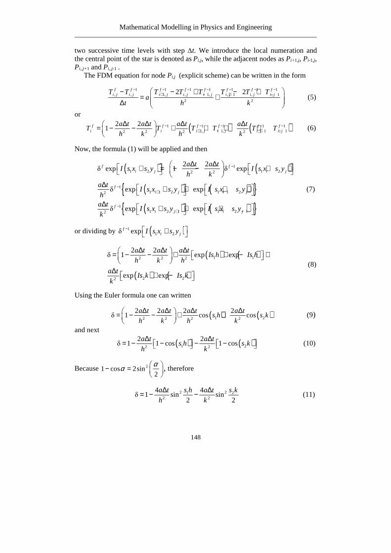
Mathematical Modelling in Physics and Engineering
148
two successive time levels with step ∆t. We introduce the local numeration and the central point of the star is denoted as Pi,j, while the adjacent nodes as Pi+ 1,j, Pi-1,j, Pi,,j+1 and Pi,,j-1 .
The FDM equation for node Pi,j (explicit scheme) can be written in the form
1 1 1 1 1 1 1, , 1, , 1, , 1 , , 1
2 2
2 2f f f f f f f fi j i j i j i j i j i j i j i jT T T T T T T T
at h k
− − − − − − −+ − + − − − + − +
= + ∆ (5)
or
( ) ( )1 1 1 1 11, 1, , 1 , 12 2 2 2
2 21f f f f f f
i i i j i j i j i j
a t a t a t a tT T T T T T
h k h k− − − − −
+ − + −∆ ∆ ∆ ∆ = − − + + + +
(6)
Now, the formula (1) will be applied and then
( ) ( )
( ) ( ) ( ) ( )
11 2 1 22 2
11 1 2 1 1 22
11 2 1 1 2 12
2 2δ exp 1 δ exp
δ exp exp
δ exp exp
f fi j i j
fi j i j
fi j i j
a t a tI s x s y I s x s y
h k
a tI s x s y I s x s y
ha t
I s x s y I s x s yk
−
−+ −
−+ −
∆ ∆ + = − − + +
∆ + + + +
∆ + + +
(7)
or dividing by ( )11 2δ expf
i jI s x s y− +
( ) ( )
( ) ( )
1 12 2 2
2 22
2 2δ 1 exp exp
exp exp
a t a t a tIs h Is h
h k h
a tIs k Is k
k
∆ ∆ ∆ = − − + + − +
∆ + −
(8)
Using the Euler formula one can written
( ) ( )1 22 2 2 2
2 2 2 2δ 1 cos cos
a t a t a t a ts h s k
h k h k
∆ ∆ ∆ ∆ = − − + +
(9)
and next
( ) ( )1 22 2
2 2δ 1 1 cos 1 cos
a t a ts h s k
h k
∆ ∆= − − − − (10)
Because 21 cos 2sin2
− =
αα , therefore
2 21 22 2
4 4δ 1 sin sin
2 2
s h s ka t a t
h k
∆ ∆= − − (11)

Mathematical Modelling in Physics and Engineering
149
The condition ,θ 1fi j < leads to the system of inequalities
2 21 22 2
4 4sin sin 0
2 2
s h s ka t a t
h k
∆ ∆+ > (12)
and
2 21 22 2
2 21 sin sin 0
2 2
s h s ka t a t
h k
∆ ∆− − > (13)
The first of them is the unconditional inequality, while the worst situation in the
case of the second inequality takes place when 2 21 2sin 1 , sin 12 2
s h s k= = and then
2 2
2 21 0
a t a t
h k
∆ ∆− − > (14)
In this way the well-known stability condition for the linear parabolic equations is found. The physical interpretation of the last formula can be found in [3].
Keywords: finite difference method, stability condition, Von Neumann method
References
[1] Tzou D. Y., Macro- to microscale heat transfer: The lagging behaviour, John Wiley & Sons, Ltd., 2015.
[2] Anderson J.D., Computational fluid dynamics. The basics with applications, McGrawHill, 1994.
[3] Mochnacki B., Suchy J.S., Numerical methods in computations of foundry processes, PFTA, Cracow, 1995.

Mathematical Modelling in Physics and Engineering
150

Mathematical Modelling in Physics and Engineering
151
EFFECT OF TORSIONAL RIGIDITY BETWEEN ELEMENTS ON FREE VIBRATIONS OF A TELESCOPIC HYDRAULIC CYLINDER
SUBJECTED TO EULER’S LOAD
Sebastian Uzny, Łukasz Kutrowski
Institute of Mechanics and Machine Design Fundamentals, Czestochowa University of Technology, Czestochowa, Poland
[email protected], [email protected]
Hydraulic cylinders are certain kinds of motors, which converts the energy of pressurized hydraulic fluid to mechanical energy. For different number of stages, one-stage and multi-stage (telescopic) hydraulic cylinders can be found. This paper revolves around boundary problem of free vibrations of a hydraulic telescopic cylinder, subjected to Euler’s load. The computational model, formulated by Tomski, which refers to free transversal vibrations and static stability of cylinders were taken into account during the calculations [1]. Effect of torsional rigidity between following elements on characteristic curves was taken into analysis in this work.
Scheme of hydraulic telescopic cylinder is presented in Fig. 1. The analysed system consist of n cylinders and piston rod. Hydraulic cylinder is analysed as a fully extended and simply supported on both ends. Overall length of the structure is defined as lC. Torsional rigidity of following elements (sealing and guiding) was modelled by rotational springs of CRi stiffness. Stiffness of rotational springs are as follows: CR1 = CR2 = CR3 = CR4 = CR5 = CR.
Diameter of the cylinders (outer dzi and inner dwi) were defined as:
2( ) 2( ) ; 2( ) 2( 1)zi t U R wi t U Rd d n i g n i g d d n i g n i g= + − + − = + − + − − (1a,b)
where gU - thickness of sealing element; gR thickness of cylinder. Each element of the hydraulic cylinder is characterized by adequate flexural
rigidity (EJ)i and mass per length unit (ρA)i. Mass of the hydraulic fluid, which fills the cylinders is (ρA)ci ((ρA)cn = 0), masses of sealing and guiding elements mi were taken into consideration. Elements of the structure marked as i = 1,2,…,n-1 correspond to cylinders and the n-element correspond to piston rod.
Results of numerical simulations, of free vibrations of the considered telescopic hydraulic cylinder were presented in the non-dimensional form , defined as:
( ) ( )( )( )
2 42*; ; ; ; CU R C C nR
GU GRt t n n n
A lg C l Plgc
d d EI EI EI
ω ρζ ζ λ= = = = Ω = (2a-e)

Mathematical Modelling in Physics and Engineering
152
Fig. 1. Scheme of n-stage telescopic hydraulic cylinder subjected to Euler’s load
Fig. 2. Characteristic curves on non-dimensional plane for different parameters of stiffness between elements
On the basis of the obtained results it can be concluded that stiffness of the sealing and guiding elements has great influence on vibration frequency and critical load. The smaller rotational node stiffness the greater its influence on vibration frequency and critical load. On the basis of the proposed non-dimensional parameters the obtained relation load – vibration frequency is linear. The characteristic curves are parallel to each other at considered configuration of the system.
Keywords: free vibrations, hydraulic telescopic cylinder, slender system
References
[1] Tomski L., Elastic Carrying Capacity of a Hydraulic Prop, Engineering Transactions 1977, 25(2), pp. 247-263.

Mathematical Modelling in Physics and Engineering
153
ANALITICAL AND NUMERICAL SOLUTION OF THE HEAT CONDUCTION PROBLEM IN THE ROD
Ewa Węgrzyn-Skrzypczak 1, Tomasz Skrzypczak 2
1Institute of Mathematics, Czestochowa University of Technology, 2 Institute of Mechanics and Machine Design Fundamentals, Czestochowa University of Technology,
Czestochowa, Poland [email protected], [email protected]
In this paper the problem of heat flow in the finite rod of length l lying on the x-axis is presented. The ends of the rod are located respectively in points 0=Ax
and lxB = . The beginning A of the rod is thermally insulated, while at its end B is
kept constant temperature 0T . It was assumed that the cross-sectional dimensions of the rod are small enough, that at all its points temperature at any given time is the same. At the initial time 0=t temperature distribution T along the rod is defined by the function )(xf , where ( )lx ,0∈ . Changing the temperature in the rod is a function of position and time ),( txTT = [1]. The scheme of the problem is presented in Fig. 1.
T
Fig. 1. Scheme of the problem
The transient heat transfer in the rod is described by the equation of heat conduction in the form [2, 3]:
2
22
T Ta
t x
∂ ∂=∂ ∂
(1)
in which
T
x xA= 0 xB= l
T0
T(x,0)

Mathematical Modelling in Physics and Engineering
154
ρλc
a =2 (2)
where: T ]K[ – temperature, t ]s[ – time, λ
msK
J – the coefficient of thermal
conductivity, c
kgKJ
– specific heat, ρ
3m
kg– density.
Equation (1) is supplemented by the boundary conditions of the first and second kind [2, 3]:
0),( TtlT = , (3)
( )
0,0 =
∂∂
x
tT (4)
The initial condition is also defined:
( ) )(0, xfxT = (5)
In order to determine an analytical solution of equation (1), under such the boundary conditions (3), the new function ( )txs , is introduced:
sTT += 0 (6)
Consequently, the boundary conditions (3)-(4) take the form:
( ) 0, =tls (7)
( )
0,0 =
∂∂
x
ts (8)
while the initial condition:(5)
( ) 0)(, Txftxs −= (9)
To obtain an analytical solution of equation (1) of form:
2
22
x
sa
t
s
∂∂=
∂∂
(10)
Fourier method is used [4]. A particular solution of the equation (10) in the form of the function of two variables is sought, where the first depends on x while the second is the function of t . When the function ( )txs , is found then condition (9) is
Mathematical Modelling in Physics and Engineering
155
used. Assuming that 0)( =xf the following analytical solution of equation (1) is obtained:
( ) 1
1
00 1cos
12
14 22 +∞
=
− −−
−= ∑ n
nn
ta xen
TTT n γ
πγ (11)
where: ( )l
nn 212
πγ −= for ,...2,1=n .
To obtain a numerical solution of equation (1) the finite element method is used. Equation (1) is multiplied by the weighting function w and integrated over the length of the rod:
02
2
=∂∂−
∂∂
∫∫B
A
B
A
x
x
x
x
dxt
Twcdx
x
Tw ρλ (12)
Using integration by parts (13)-(14) the first term in equation (12) may be written in the form (15).
B
A
B
A
B
A
x
x
x
x
x
x
uvdxvuvdxu +′−=′ ∫∫ (13)
.,
,,2
2
dx
dwv
x
Tu
wvx
Tu
=′∂∂=
=∂∂=′
λ
λ (14)
∫∫ ∂∂+
∂∂−=
∂∂ B
A
B
A
B
A
x
x
x
x
x
xx
Twdx
x
T
dx
dwdx
x
Tw λλλ
2
2
(15)
Heat flux at the points Ax and Bx is defined as follows:
b
a
B
A
x
x
x
x
qdx
dT =− λ (16)
Finally the weak form of the equation of heat conduction takes the following form:
b
a
x
xqwdx
t
Twcdx
x
T
x
w −=∂∂+
∂∂
∂∂
∫∫ΩΩ
ρλ (17)
Equation (17) is discretized over the space with the use of the Galerkin method where the weighting functions w are the same as the shape functions N of the
Mathematical Modelling in Physics and Engineering
156
finite elements. Then the implicit time integration scheme is used to obtain global set of equations. The final form of the global FEM equation is shown below:
ff
ttMTBTMK
∆+=
∆+ + 11 1 (18)
where: K is the global thermal conductivity matrix, M – global heat capacity matrix, B – right hand side vector, t∆ – time step, f – time level.
In this paper results of analytical solution obtained using the Fourier series and numerical model based on the Finite Element Method for selected time moments are presented. In addition, distributions of the temperature obtained as a result of both solutions, are compared to check their compatibility. The solutions of equation (1) are obtained using the boundary conditions (3)-(4) and the initial condition (5) for certain material properties.
Keywords: heat conduction equation, Fourier’s method, Finite Element Method
References
[1] Zaporożec G., Metody rozwiązywania zadań z analizy matematycznej, WNT, Warszawa, 1967. [2] Longa W., Krzepnięcie odlewów w formach piaskowych, Wydawnictwo „Śląsk”, 1973. [3] Mochnacki B., Suchy J., Modelowanie i symulacja krzepnięcia odlewów, PWN, Warszawa,
1993. [4] Fichtenholz G. M., Rachunek różniczkowy i całkowy, PWN, Warszawa 1999.

Mathematical Modelling in Physics and Engineering
157
INFLUENCE OF GROOVE WELD ON RESIDUAL STRESSES IN SINGLE-PASS BUTT WELDED JOINTS WITH THOROUGH
PENETRATION
Jerzy Winczek, Krzysztof Makles
Institute of Mechanical Technologies, Czestochowa University of Technology, Czestochowa, Poland
[email protected], [email protected]
A chamfering of the joining sheet edges is often used in welding practice. In work, the analysis of groove weld influence on residual stress distribution in single-pass butt welded joints with thorough penetration, is presented.
Welding is characterised by an application of the movable, concentrated heat source which action causes temperature field movable in time and space. The point of departure in the description of the temperature field in a homogeneous and isotropic body is a basic differential equation of heat conduction based on the law of conservation of energy [1]. Analytical method, proposed by Geissler and Bergmann [2], was chosen to solve this differential equation. Three-dimensional temporary field for butt welding with thorough penetration was determined on the basis of analytical methods of an integral transformation and Green’s function.
Heating processes of steel leads to the transformation of primary structure into austenite, while cooling leads to the transformation of austenite into ferrite, pearlite, bainite and martensite. Structural changes of welded joint, connected with its cooling (also with hardening), develop heterogeneous picture of material structure, which influences the state of stress after welding. Kinetics of phase transformations during heating is limited by temperature values at the beginning and at the end of austenitic transformation. The quantitative progress of phase transformations during welding is determined on the Johnson-Mehl-Avrami and Kolomogorov law for diffusive transformations [3], and the Koistinen-Marburger law for martensitic transformation [4]. The description of the dependence of material’s structure, temperature and transformation time of over-cooled austenite during surfacing is made in accordance with the TTT (time-temperature-transformation) welding diagram during continuous cooling.
The structural strains resulting from different densities of individual structures are related to phase transformations, which in conjunction with the thermal strains leads to complicated history of strains during welding thermal cycle. In strain calculations there was assumed a linear expansion coefficient of particular structural elements and structural strains. Total strain during single-pass welding represents the sum of thermal strains caused by phase transformation during heating and cooling. Heating leads to the increase in material’s volume, while transformation of the initial structure (ferritic, pearlitic or bainitic) in austenite causes shrinkage connected with different density of given structures. Cooling of

Mathematical Modelling in Physics and Engineering
158
material causes its shrinkage, while transformation of austenite in cooling structures causes in turn the increase of its volume. It leads to complicated changes of strains dependent not only on the current temperature of material during cooling but also on the initial and final temperature of transformation of austenite into ferrite, pearlite, bainite or martensite as well as on volumetric shares of given structural constituents (including austenite).
Analytical model of temporary and residual stresses for butt welding with thorough penetration was described assuming planar section hypothesis and using integral equations of stress equilibrium of the bar and simple Hooke’s law. In solution the effect of temperature and phase transformations (structure changes and structural strains) has been taken into account.
Computations of temporary temperature field, phase transformations, strains and stresses have been conducted for one-side butt welded of two flats made from S235 steel. Numerical simulations were made for joint with welding groove and for joint without chamfering of flats. For calculations are used authors’ programs made in Borland Delphi. The results are presented in the form of temperature, volume phase fraction and stress distributions in the element’s cross section as well as stress history at selected points.
The analysis of residual stress distribution after welding of flats for joint with welding groove and for join without chamfering of sheets, did not show significant differences. The tensile stress values in the weld and the heat affected zone are similar, as is the stress distribution in the area of the parent material. This is due to a complete melting of the joint area (liquid area), and the final stress state arises after the weld solidification. It follows that the weld groove in the geometric model of an welded object for the stress state calculation during butt welded joints with thorough penetration, can be omitted.
Keywords: mathematical modelling, butt welded joint, groove weld, stresses
References
[1] Carslaw H.S, Jaeger J.C., Conduction of heat in solids. Oxford University Press 1973. [2] Geissler E., H.W. Bergmann H.W., Calculation of temperature profiles heating and quenching
rates during laser processing, Optoelektronik Magazin, 1987, 3(4), 430 – 434. [3] Piekarska W, Kubiak M, Bokota A. Numerical simulation of thermal phenomena and phase
transformations in laser-arc hybrid welded joint. Archiv Metall Materials. 2011;56:409-421. [4] Domański T., A. Bokota A., Numerical models of hardening phenomena of tools steel base on
the TTT and CCT diagrams, Archiv. Metall. Mater. 2011, 56, 325 – 344. [5] Winczek J., The analysis of stress states in steel rods surfaced by welding, Archiv. Metall.
Mater., 2013, 58, 1243 – 1252.
Mathematical Modelling in Physics and Engineering
159
QUEUEING SYSTEMS WITH LIMITED BUFFER SPACE AND LIMITED QUEUEING TIME
Paweł Zając 1, Oleg Tikhonenko 2 1Institute of Mathematics, Czestochowa University of Technology,
Czestochowa, Poland 2Faculty of Mathematics and Natural Sciences, College of Sciences,
Cardinal Stefan Wyszyński University in Warsaw Warszawa, Poland
[email protected], [email protected]
We investigate queueing systems with demands of random space requirements and limited buffer space, in which queueing or sojourn time are limited by some constant value. For such systems, in the case of exponentially distributed service time and Poisson entry, we obtain the steady-state demands number distribution and probability of demands losing. In our work, we study queueing systems in which demands are also “impatient”. In other words, they can leave the system during their waiting in the queue, or even during their servicing. Such systems are the models of some real processes. E.g., systems of information transmission often deal with the process of messages information reduction.
Consider the / / /M M n m≤ ∞ - type queueing system with identical servers and FIFO service discipline. Let a be the intensity of demands entrance flow, µ be
the parameter of service time. Each demand has some random volume ζ which does not depend on the volumes of other demands nor on the demand arriving epoch. Let ( ) P <xL x ζ= be the demand volume distribution function and ( )tσ be the sum of volumes of all demands present in the system at time instant t . The values of the process ( )tσ are limited by the constant value V (buffer space
capacity). Let us denote by )(tη the number of demands present in the system at time t. Let a demand having the volume x arrive to the system at epoch t. Then, it will be accepted to the system if ( )t n mη − < + and ( )t x Vσ − + ≤ . In this case, we
have ( ) ( ) 1t tη η −= + , ( ) ( )t t xσ σ −= + . In opposite case, the demand will be lost and
( ) ( )t tσ σ −= , ( ) ( )t tη η −= . If t is the epoch when a demand of volume x leaves the
system, we have ( ) ( ) 1t tη η −= − , ( ) ( )t t xσ σ −= − .
We will assume that the system load = a ([n( + )]) ρ µ α is finite (ρ < ∞ ). Our goal is to determine the distribution of the stationary number of entries that are present in the system and the probability of reporting loss due to these restrictions.
Let A be the event that the request that came to the system stationary will not be lost at the time of its arrival and will continue to be completely served, K - average number of occupied service devices (positions). It is clear that

Mathematical Modelling in Physics and Engineering
160
∑ ∑=
+
+=
+=n
k
mn
nkkk pnkpK
1 1
.
Then the probability that the requests will be lost at the time of arrival or not fully served is
ρµ
µµ)(
111an
K
a
KAPloss +
−=−=Ρ−= .
For example, when the volume of the requests has a uniform distribution on the interval ]2,1[ , then the probability of its loss is given by the graph (figure 1).
Fig. 1. Loss probability for ]10,0[=V
Keywords: queueing system, buffer space capacity, demand volume, queueing time
References
[1] Gnedenko B.V., Kovalenko I.N., Introduction to Queueing Theory, Birkhäuser, Boston 1989. [2] Tikhonenko O., Computer Systems Probability Analysis, Akademicka Oficyna Wydawnicza
EXIT, Warsaw 2006 (in Polish). [3] Tikhonenko O., Zajac P.: Queueing Systems with Demands of Random Space Requirement and
Limited Queueing or Sojourn Time. In: Gaj P., Kwiecień A., Sawicki M. (eds) Computer Networks. CN 2017. Communications in Computer and Information Science, vol. 718, pp. 380-391. Springer, Cham 2017. doi: 10.1007/978-3-319-59767-6_30