Mathematical modelling of concrete - Simon Fraser …people.math.sfu.ca/~stockie/papers/Talks/caims10.pdfIntroduction Mathematical model Numerical simulations Mathematical modelling

IntroductionMathematical model

Numerical simulations

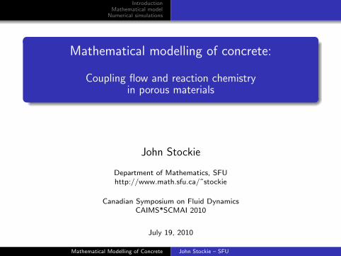
Mathematical modelling of concrete:

Coupling flow and reaction chemistryin porous materials

John Stockie

Department of Mathematics, SFUhttp://www.math.sfu.ca/˜stockie

Canadian Symposium on Fluid DynamicsCAIMS*SCMAI 2010

July 19, 2010

Mathematical Modelling of Concrete John Stockie – SFU



Acknowledgments

Michael Chapwanya

Postdoctoral fellow

Currently an Assistant Professor at Universityof Pretoria

Wentao Liu

Summer undergraduate research assistant

Currently a PhD student at University ofWaterloo

Funded by:




Outline

1 IntroductionWhat is concrete?Concrete composition and chemistryMotivation: Re-wetting experiments

2 Mathematical modelPhysical set-upGoverning equations

3 Numerical simulationsClogging simulationSensitivity study




What is concrete?Concrete composition and chemistryMotivation: Re-wetting experiments

Outline








Why study concrete?

Concrete has a reputation as a “low tech” material, but it isactually very complex and worthy of study! Furthermore . . .

It’s the most widely used construction material in the world.In 1997, 6.4B m3 was produced – that’s 2.5 T per person!Of any material, only water has a higher consumption rate.It’s a climate change villain: the cement industry produces5–10% of man-made CO2 globally.





Cement versus concrete?

The words “cement” and “concrete” are frequentlymisused/confused.

Cement:Is a binding agent that hardens andholds other materials together.Ingredients: limestone, clay, gypsum,and other additives.

Concrete:Is a mixture of cement, aggregate(gravel or crushed stone), sand, andwater.Concrete hardens after mixing withwater through a process calledhydration.





Concrete composition

A typical concrete mix: cement (11%), gravel (41%),sand (26%), water (16%) and air voids (6%).

This composition changes over time as the cement hydratesand concrete hardens.





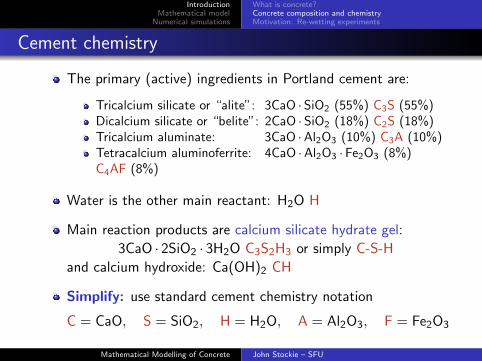
Cement chemistry

The primary (active) ingredients in Portland cement are:

Tricalcium silicate or “alite”: 3CaO ·SiO2 (55%) C3S (55%)Dicalcium silicate or “belite”: 2CaO ·SiO2 (18%) C2S (18%)Tricalcium aluminate: 3CaO ·Al2O3 (10%) C3A (10%)Tetracalcium aluminoferrite: 4CaO ·Al2O3 ·Fe2O3 (8%)C4AF (8%)

Water is the other main reactant: H2O H

Main reaction products are calcium silicate hydrate gel:

3CaO · 2SiO2 · 3H2O C3S2H3 or simply C-S-H

and calcium hydroxide: Ca(OH)2 CH

Simplify: use standard cement chemistry notation

C = CaO, S = SiO2, H = H2O, A = Al2O3, F = Fe2O3





Cement chemistry 2

Main reactions for alite and belite:

2C3S + 6Hra−→ C-S-H (aq) + 3CH

2C2S + 4Hrb−→ C-S-H (aq) + CH

Note: Alite reaction is much faster than belite: ra � rb

Precipitation/dissolution: gel forms from aqueous C-S-H

C-S-H (aq)kprec−−⇀↽−−kdiss

C-S-H (gel)





Cement chemistry 3

Initial hydration: formationof crystalline “fingers” onsilicate grains.

Setting: over a period ofhours, C-S-H gel matrixforms rapidly.

Clogging: C-S-H gel causesporosity to decrease.

Hardening/curing:hydration continues for daysand even months.





Concrete structure

Hardened concrete has a complex, multi-scale porous structure with

gel pores (10–100 nm) � capillary pores (10 µm) � air voids (1 mm)





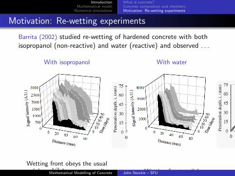
Motivation: Re-wetting experiments

Barrita (2002) studied re-wetting of hardened concrete with bothisopropanol (non-reactive) and water (reactive) and observed . . .

With isopropanol With water

Wetting front obeys the usualxf (t) ∝ t1/2 for porous media

flow.Wetting front stalls!

Wetting front penetrates sample at a rate that decreases with timeAND water behaves differently from isopropanol.





Main hypothesis

Hypothesis (from experimentalists):

Re-hydration of residual (unreacted) silicates leads to C-S-H gelformation that in turn clogs capillary pores.

Note:

Initial hydration and setting phases have been modelledextensively, e.g. Bentz et al. (1994), Tzschichholz et al. (1995),Preece et al. (2001), etc.

Hall et al. (1995) present experimental evidence that re-wettingleads to “anomalously low absorption rates.”

However, re-wetting has not been modelled to date.




Physical set-upGoverning equations

Outline








Barrita’s re-wetting experiment

Barrita, Bremner & Balcom (2003):

A long, thin, cylindricalsample of dry concrete.

Sides are sealed.

Bottom is placed in a liquidreservoir.

Wetting front movesupwards due to capillaryaction.

Use magnetic resonanceimaging to determine frontlocation.

��

��

wetting front

reservoir

( << 1 )θ

saturated medium( = 1 )

dry medium

θ





Main assumptions

1 Problem is one-dimensional (sample is long and thin).

2 Liquid transport obeys Darcy’s law (capillary pore scale only).

3 No temperature variations (reactions are slow).

4 Gravity is negligible (pores are small, low Bo = ρgL2

γ ).

5 Consider only silicate reactions (C3S and C2S make up70–80% of active ingredients).

6 Neglect individual ionic species.

7 Ignore chemical shrinkage.





Variables

Define the following dependent variables:

θ(x , t) = liquid saturation

Ca(x , t) = C3S (alite) concentration

Cb(x , t) = C2S (belite) concentration

Cq(x , t) = aqueous C-S-H concentration

Cg (x , t) = solid C-S-H gel concentration

An important supplementary variable is porosity:

ε(x , t) = εo −Cg (x , t)

ρg





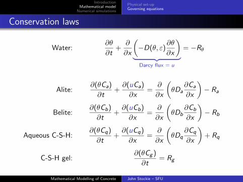
Conservation laws

Water:∂θ

∂t+

∂

∂x

(−D(θ, ε)

∂θ

∂x

)︸︷︷︸

Darcy flux = u

= −Rθ

Alite:∂(θCa)

∂t+

∂(uCa)

∂x=

∂

∂x

(θDa

∂Ca

∂x

)− Ra

Belite:∂(θCb)

∂t+

∂(uCb)

∂x=

∂

∂x

(θDb

∂Cb

∂x

)− Rb

Aqueous C-S-H:∂(θCq)

∂t+

∂(uCq)

∂x=

∂

∂x

(θDq

∂Cq

∂x

)+ Rq

C-S-H gel:∂(θCg )

∂t= Rg





Reaction termsConsumption of alite: Ra = kaC

naa (θ − θmin)+︸︷︷︸

= min(θ−θmin,0)(“shut-off”)

Consumption of belite: Rb = kbCnbb (θ − θmin)+

Generation of C-S-H (aq + gel):(weighted by molar masses)

Rcsh =mcsh

2

(Ra

ma+

Rb

mb

)

Generation of water: Rθ = kθRcsh

Generation of C-S-H (aq): Rq = Rcsh − Rg

Generation of C-S-H (gel):(precipitation and dissolution)

Rg = (kprecCq − kdissCg )(θ − θmin)+





Water diffusion coefficient

D(θ, ε) = AeBθ

(ε− θmin

εo − θmin

)19/6 (ε− θmin

εo − θmin

)19/6

︸︷︷︸clogging

0 0.2 0.4 0.6 0.8 10

0.5

1

1.5

2

! = ("!"min)/("max!"min)

D(!

) [c

m2 /d

ay]

Exponential dependence on θ is fit to concrete experiments,with B ≈ 6 and A ≈ 0.003.

Saturation is governed by a nearly degenerate diffusionequation with some interesting mathematical properties. . . later . . .

The second factor represents clogging, and is commonlyemployed for biofilms in soil (Clement et al., 1996).





Parameter values

Typical values of a few of the most important parameters:

Sample length: L = 10 cm.

Diffusivity: B = 6 and A = 0.003.

Narrow range of saturation: θmin = 0.04, θmax = εo = 0.067.

Reaction exponents: na = 2.65, nb = 3.10.

Reaction rates: ka = 22.2 d−1, kb = 3.04 d−1.

Precipitation/dissolution rates: kprec = 32.2 d−1, kdiss = 0.

Refs: Papadakis et al. (1989), Bentz (2006).




Clogging simulationSensitivity study

Outline








Solution algorithm

Employ a method of lines approach with a second-ordercentered finite volume discretization in space.

Use N = 100 grid points in space, which yields a couplednonlinear system of 5N ODEs in time.

Solve using Matlab’s stiff solver ode15s.

Requires less than 1 min. on a Mac PowerBook.





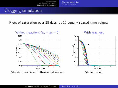
Clogging simulation

Plots of saturation over 28 days, at 10 equally-spaced time values:

Without reactions (ka = kb = 0) With reactions

Standard nonlinear diffusive behaviour. Stalled front.





Clogging simulation 2

Discrepancy between initial slopes for water/isopropanol datais likely due to variations in samples used.Results are fit to water data using two parameters:

Choose A = 0.003 cm2/day to match wetting front speed.Scale reaction rates to match stalling location.





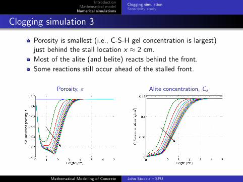
Clogging simulation 3

Porosity is smallest (i.e., C-S-H gel concentration is largest)just behind the stall location x ≈ 2 cm.

Most of the alite (and belite) reacts behind the front.

Some reactions still occur ahead of the stalled front.

Porosity, ε Alite concentration, Ca





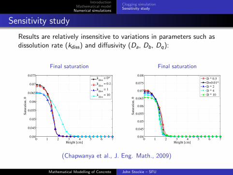
Sensitivity study

Results are relatively insensitive to variations in parameters such asdissolution rate (kdiss) and diffusivity (Da, Db, Dq):

Final saturation Final saturation

0 1 2 3 4 5 6 70.04

0.045

0.05

0.055

0.06

0.065

0.07

0.075

Height [cm]

Satu

ratio

n, !

kdiss = 0*kdiss = 0.1kdiss = 1kdiss = 10

0 1 2 3 4 5 6 70.04

0.045

0.05

0.055

0.06

0.065

0.07

0.075

0.08

Height [cm]

Satu

ratio

n, !

D * 0.5D=0.01*D * 2D * 4D * 10

(Chapwanya et al., J. Eng. Math., 2009)





Sensitivity study 2

Results much more sensitive to changes in reaction rates (kα, kβ):

Final saturation Wetting front position

0 1 2 3 4 5 6 7

0.04

0.045

0.05

0.055

0.06

0.065

0.07

Height [cm]

Satu

ratio

n, !

k"

= 0k"

= 2.22k"

= 22.2*k"

= 222

0 1 2 3 4 50

1

2

3

4

5

6

7

Time [day1/2]Fr

ont p

ositi

on [c

m]

k!

= 0k!

= 2.22k!

= 22.2*k!

= 222

(Chapwanya et al., J. Eng. Math., 2009)




Summary & Conclusions

Developed a model for transport and reaction of water andsilicates in hardened concrete.

Calibration and comparison to a very detailed set ofexperiments.

Numerical simulations support the hypothesis that hydrationof residual silicates is responsible for anomalous watertransport observed in re-wetting experiments.

Sensitivity studies identify the most important physicalparameters.




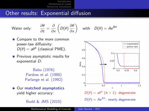
Other results: Exponential diffusion

Water only:∂θ

∂t=

∂

∂x

(D(θ)

∂θ

∂x

)with D(θ) = AeBθ

Compare to the more commonpower-law diffusivity:D(θ) = aθb (classical PME).

Previous asymptotic results forexponential D:

Babu (1976)Parslow et al. (1988)Parlange et al. (1992)

Our matched asymptoticsyield higher accuracy:

Budd & JMS (2010)

0 0.5 1 1.50

0.2

0.4

0.6

0.8

1

x

thet

a

exponentialpower!law

0.5 0.55 0.60

0.05

0.1

D(θ) = aθb (b > 1): degenerate

D(θ) = AeBθ: nearly degenerate




Future work

Further experiments are necessary to confirm our hypothesisabout hydration of residual silicates (work with Barrita).

Incorporate transport and reaction kinetics of individual ionicspecies, similar to other models of initial hydration,carbonation (Meier et al., 2007), and chlorination (Papadakis et

al., 1992).

Derive analytical results on wetting front motion and stalllocation, a la Muntean & Bohm (2006).

Numerical studies of the related phenomenon ofself-desiccation and associated shrinkage effects.

Applications: high-performance concrete, monumentdegradation and restoration, etc.




References I

D. K. Babu.

Infiltration analysis and perturbation methods. 1. Absorption withexponential diffusivity.

Water Resour. Res., 12(1):89–93, 1976.

P. Barrita.

Curing of high-performance concrete in hot dry climates studied usingmagnetic resonance imaging.

PhD thesis, University of New Brunswick, Fredericton, NB, Nov. 2002.

P. Barrita, T. W. Bremner, and B. J. Balcom.

Effects of curing temperature on moisture distribution, drying and waterabsorption in self-compacting concrete.

Mag. Concr. Res., 55(6):517–524, 2003.




References II

D. P. Bentz.

Influence of water-to-cement ratio on hydration kinetics: Simple modelsbased on spatial considerations.

Cement Conc. Res., 36(2):238–244, 2006.

D. P. Bentz, P. V. Coveney, E. J. Garboczi, M. F. Kleyn, and P. E.Stutzman.

Cellular automaton simulations of cement hydration and microstructuredevelopment.

Modelling Simul. Mater. Sci. Eng., 2:783–808, 1994.

C. J. Budd and J. M. Stockie.

Asymptotic behaviour of wetting fronts in porous media with exponentialmoisture diffusivity.

In preparation, 2010.




References III

M. Chapwanya, W. Liu, and J. M. Stockie.

A model for reactive porous transport during re-wetting of hardenedconcrete.

J. Eng. Math., 65(1):53–73, 2009.

T. P. Clement, B. S. Hooker, and R. S. Skeen.

Macroscopic models for predicting changes in saturated porous mediaproperties cause by microbial growth.

Ground Water, 34(5):934–942, 1996.

C. Hall, W. D. Hoff, S. C. Taylor, M. A. Wilson, B.-G. Yoon, H.-W.Reinhardt, M. Sosoro, P. Meredith, and A. M. Donald.

Water anomaly in capillary liquid absorption by cement-based materials.

J. Mater. Sci. Lett., 14:1178–1181, 1995.




References IV

S. A. Meier, M. A. Peter, A. Muntean, and M. Bohm.

Dynamics of the internal reaction layer arising during carbonation ofconcrete.

Chem. Eng. Sci., 62:1125–1137, 2007.

A. Muntean and M. Bohm.

Length scales in the concrete carbonation process and water barrier effect:A matched asymptotics approach.

Report No. 06-07, Zentrum fur Technomathematik, Universitat Bremen,Sept. 2006.

V. G. Papadakis, M. N. Fardis, and C. G. Vayenas.

Hydration and carbonation of pozzolanic cements.

ACI Mater. J., 89(2):119–130, 1992.




References V

V. G. Papadakis, C. G. Vayenas, and M. N. Fardis.

A reaction engineering approach to the problem of concrete carbonation.

AIChE J., 35(10):1639–1650, 1989.

M. B. Parlange, S. N. Prasad, J.-Y. Parlange, and M. J. M. Romkens.

Extension of the Heaslet-Alksne technique to arbitrary soil waterdiffusivities.

Water Resour. Res., 28(10):2793–2797, 1992.

J. Parslow, D. Lockington, and J.-Y. Parlange.

A new perturbation expansion for horizontal infiltration and sorptivityestimates.

Transp. Porous Media, 3:133–144, 1988.

S. J. Preece, J. Billingham, and A. C. King.

On the initial stages of cement hydration.

J. Eng. Math., 40:43–58, 2001.




References VI

F. Tzschichholz, H. J. Herrmann, and H. Zanni.

A reaction-diffusion model for the hydration/setting of cement.

arXiv:cond-mat/9508016v1, 4 August 1995.


Documents

Mathematical modelling of concrete - Simon Fraser …people.math.sfu.ca/~stockie/papers/Talks/caims10.pdfIntroduction Mathematical model Numerical simulations Mathematical modelling