Mathematical Modelling for Synthetic Biology

aGEM Workshop on Mathematical ModellingJuly 22, 2012, Lethbridge, AB

Brian IngallsDepartment of Applied Mathematics

University of WaterlooWaterloo, ON

Workshop Outline

• Introduction to mathematical modelling of biochemical reaction networks

• Modelling of gene regulatory networks

• Lab I: simulation of kinetic models• Tools for model analysis • Lab II: model-based design of gene

regulatory networks

Models in Science and Engineering

• Models are abstractions of reality

Models in Science and Engineering

• Models are abstractions of reality• Models can be physical

Ball-and-stick model of molecular structure

http://mariovalle.name/ChemViz/representations/index.html http://srxawordonhealth.com/2012/04/

Mouse model of obesity

Models in Science and Engineering

• Models are abstractions of reality• Models can be physical or conceptual

http://www.nature.com/scitable/topicpage/gpcr-14047471

Interaction diagram model of G-protein signalling

Kinetic model of bacterial chemotaxis signalling pathway

Models in Science and Engineering

• Models are abstractions of reality• Models can be physical or conceptual • Mathematical models are

mechanistic (based on physico-chemical laws) and predictive (allow inferences beyond the data used for their construction)

How are mathematical models used in molecular biology?

• Models summarize data• Models allow of falsification of

hypotheses• Models allow exploration of system

behaviour (in silico experiments) • Model-based design allows easy

exploration of design space

Model Construction

Modelling Chemical Reaction Networks

Chemical reaction:

Rate constant:

Law of mass action:

Using derivatives to describe rates of change

Ex: decay reaction:

rate of change of [A] at time t

rate of reaction at time t

differentialequation model

Solution of the differential equation model

Model simulation = in silico experiment

Model Simulation

Numerical simulation of differential equation models

Approximate derivative by a difference quotient

Rearrange to yield an update rule:

Implemented in MATLAB, XPPAUT, Copasi, Mathematica, Maple, …

Tutorials in notes for XPPAUT (freeware, simulation and analysis of differential equation models) MATLAB (licensed, general-use computational software)

Repeated application of the update rule (starting from known initial concentration):

Example network model

network

simulationmodel

Model Analysis

Separation of time-scales

Every model is formulated around a specific time-scale

Processes occurring on a slower time-scale are treated as frozen in time

Processes occurring on a faster time-scale are presumed to occur instantaneously

Treating rapid processes

Rapid equilibrium approximation: presume at all times.

Quasi-steady-state approximation: presume [A] is in steady-state with respect to [B] at all times.

Sensitivity analysisMeasure sensitivity of steady-state species concentrations to changes in model parameters

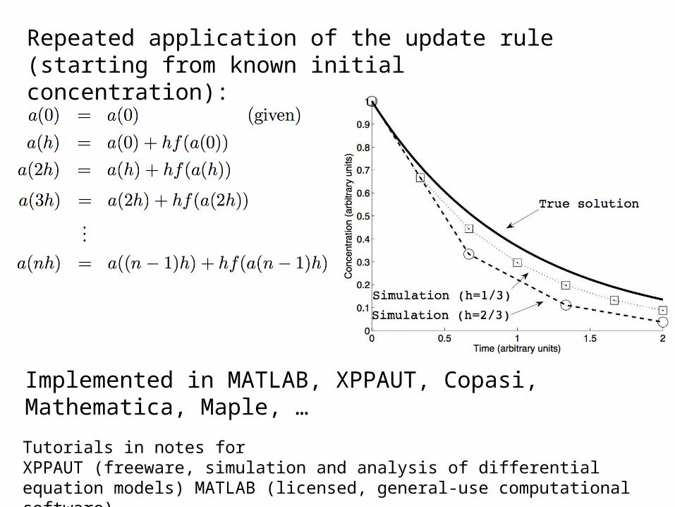
Applications of Sensitivity analysis

Identification of optimal drug targets (steps with high sensitivities)

Bakker et al. 1999, ‘What controls glycolysis in bloodstream form Trypanosoma brucei? JBC 274.

Applications of Sensitivity analysis

Interpretation of regulation schemes: role of negative feedback

Biochemical Kinetics

Saturation: Michaelis-Menten kinetics

Rates of enzyme-catalysed reactions exhibit saturation:

Michaelis-Menten kinetics

Cooperativity: Hill function kinetics

Processes involving multiple interacting components can exhibit sigmoidal activity (e.g. cooperative binding of O2 to hemoglobin)

Hill function (empirical fit)

Gene Regulatory Networks

Modelling constitutive gene expression

mRNA dynamics:

protein dynamics:

Modelling constitutive gene expression

If mRNA dynamics are fast (compared to protein dynamics): Treat mRNA in ‘quasi-steady-state’

Reduced model only describes protein concentration :

Regulated gene expression

Constitutive expression

Repressed expression

Regulated gene expression

Constitutive expression

Activated expression

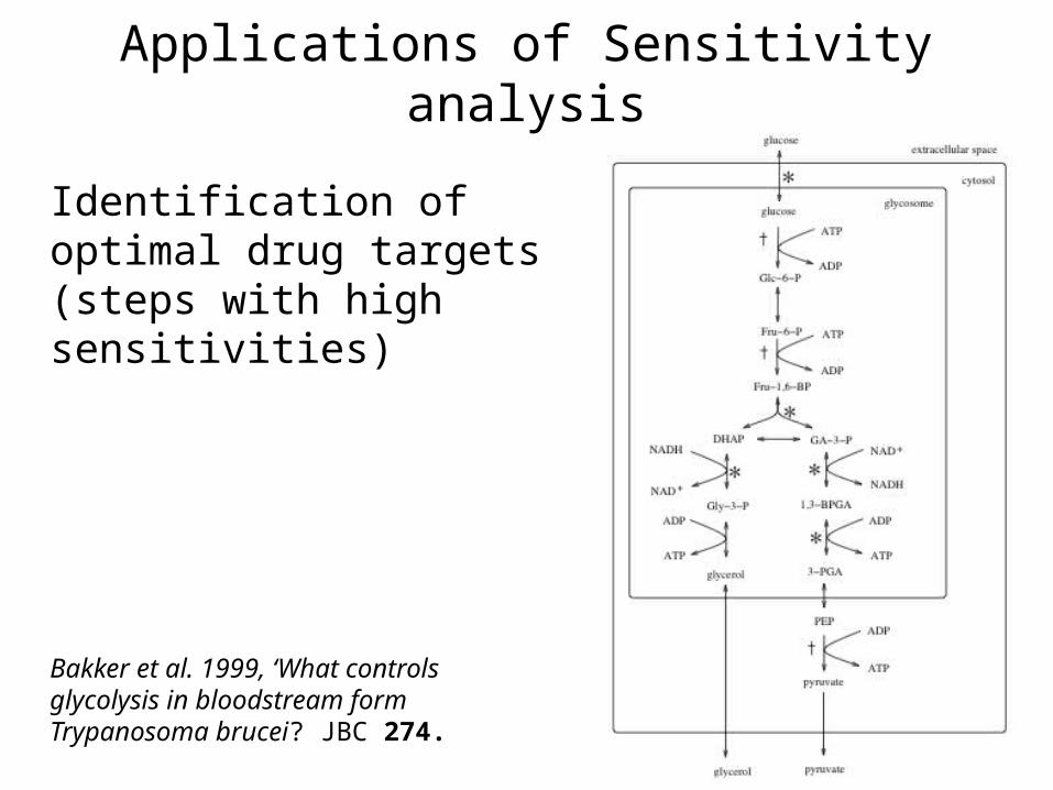
Modelling regulated expression

Modelling regulated expression

Regulation by multiple transcription factors

Distribution of states: If A=B=P, with cooperative binding:

Natural Gene Regulatory Networks

Autoregulating genes

Autorepressor: (regulation enhances robustness and response timing)

Autoactivator: (bistable ON/OFF switching behaviour)

Gene switch: lac operon

Gene autoactivates in response to lactose

Gene switch: lysis/lysogeny decision in phage lambda

crocI

Double negative feedback locks in one of two states

Oscillatory gene network: the Goodwin oscillator

Delayed negative feedback leads to sustained oscillations

Oscillatory gene network: circadian rhythm generator

Delayed negative feedback leads to sustained oscillations

Model: Goldbeter, 1996

Developmental gene networks

Endomesoderm specification in purple sea urchin (Davidson, Bolouri et al.)

Segmentation in Drosophila

Engineered Gene Circuits

The Collins Toggle SwitchGardner, Cantor, and Collins, Nature, 2000

Double repression locks in one of two possible states.

Inducers allow transitions

Collins toggle switch: implementation

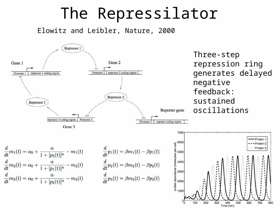
The RepressilatorElowitz and Leibler, Nature, 2000

Three-step repression ring generates delayed negative feedback: sustained oscillations

Repressilator: Implementation

pro

gen

ysi

ngle

cell

Improved oscillator design: relaxation oscillator

Interplay of positive and negative feedback lead to robust sustained rise-and-crash oscillations

Stricker/Hasty oscillatorStricker et al., Nature, 2008

Interplay of positive and

negative feedback lead to robust sustained

oscillations

Stricker/Hasty oscillator implementation

Lab I

Goals:1) Simulate a differential equation

model in XPPAUT2) Determine sensitivity coefficients for

a simple network model3) Explore system behaviour in models

of gene regulatory networks: the Collins toggle switch, the repressilator, the Hasty/Stricker oscillator

Lab I1) Simulate a differential equation model in XPPAUTa) Open XPPAUT with file Lab1.ode or generate your own file, content is simply:par k=1x’=-k*xinit x=1doneb) Select Initialconds|Go (I|G). Resize the window with Window/zoom|Fit (W|F). Then choose Initialconds|New (I|N) and run a simulation with initial value of x set to 0.5. c) Open the param window, change the value of k to 1. Re-run your simulations from x(0)=1 and x(0)=0.5. How has the behaviour changed?

2) Determine sensitivity coefficients for a simple network modela) Open XPPAUT with file Lab2.odeb) Select Initialconds|Go (I|G). Use the Data window to view all four species concentrations. Select Graphic stuff|

Add curve (G|A) to add additional time-series to the plot.c) Open the param window. Explore the effect of changing the parameter values. Consider the sensitivities of the

steady state of [A] with respect to (i) k1; (ii) k2; and (ii) k3.

3) Explore system behaviour in models of gene regulatory networks: the Collins toggle switch, the repressilator, the Hasty/Stricker oscillatora) Open XPPAUT with one of the files Lab_toggle.ode, Lab_repressilator.ode, or Lab_hastyosc.odeb) Select Initialconds|Go (I|G). Verify the system’s desired behaviour: oscillations or bistability (for bistability, modify the initial conditions).c) Explore the effect of modifying the model parameters (param window) on the desired behaviour

Tools for analysis of dynamic mathematical

models

The phase plane

Example network:

Time series: species concentrations plotted against time

Phase portrait: species concentrations plotted against one another

The phase plane

The phase plane

Time series: multiple simulations (range of initial concentrations)

Phase portrait: multiple simulations reveal system behaviour

The phase plane

Direction field Nullclines (turning points)

Intersection of nullclines: steady state.

Stability

Stability

Example: symmetric antagonistic network:

Case I: Non-symmetric inhibition strengths: unique long-time (steady-state) behaviour

Stability

Example: symmetric antagonistic network:

Case II: Symmetric inhibition strengths: two potential long-time (steady-state) behaviours

Stability

Nullclines intersect three times.

Intermediate steady-state is unstable, other two are stable.

Stability

A bistable system

Stability

monostability bistability

saddle point

Linearized Stability Analysis

Evaluate Jacobian at steady state:

Model:

Determine eigenvalues of Jacobian:

If all eigenvalues have negative real part, then the steady state is stable

Oscillations

Oscillatory behavior

Example: autocatalytic pathway:

Case I: weak autocatalysis: damped oscillations (settling to steady state)

Oscillatory behavior

Example: autocatalytic pathway:

Case II: strong autocatalysis: sustained (limit cycle) oscillations

Limit cycle

Bifurcation analysis

Bifurcation diagramsThe location of steady states depends on model parametersPlot of steady-state concentration against parameter value: continuation diagram

Bifurcation diagram: bistability

Parameter values at which the number or stability of steady states change are called bifurcation points

nullclines vary with parameter values

Bistable network

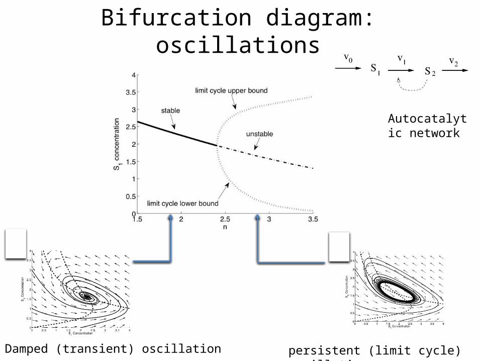
Bifurcation diagram: oscillations

Autocatalytic network

Damped (transient) oscillation persistent (limit cycle) oscillation

Model-based design

The Collins Toggle Switch

repression

repression

Network:

Goal: bistability

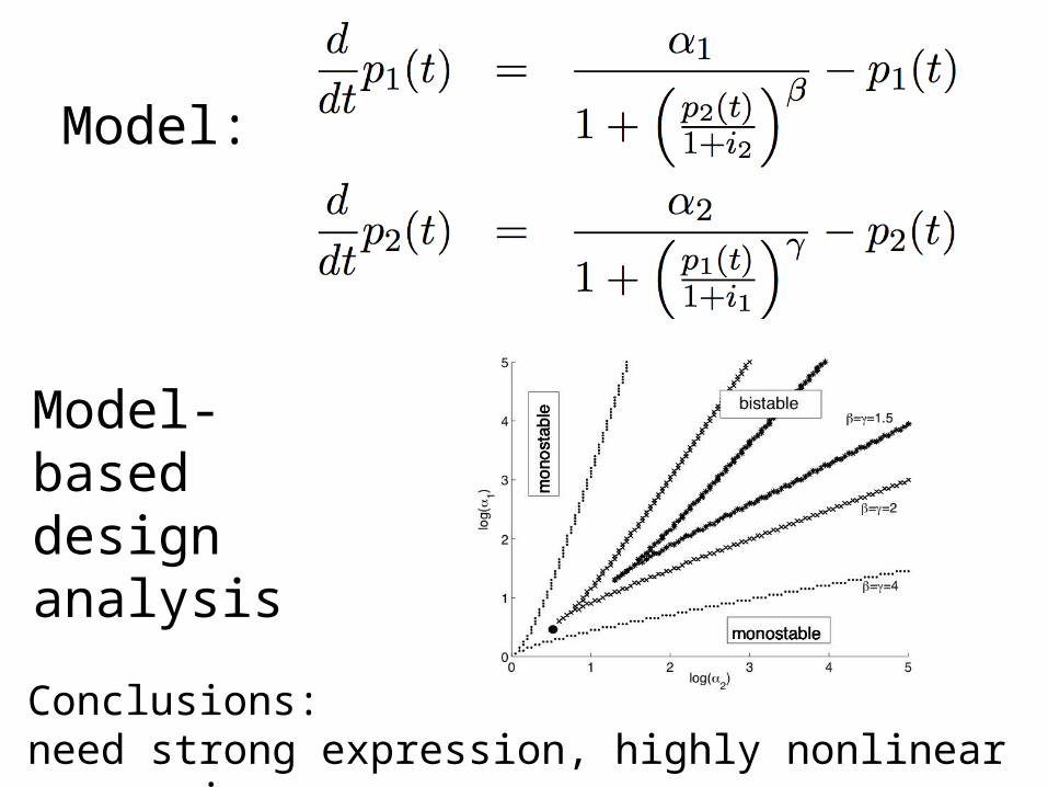
Model:

Model-based design analysis

Conclusions: need strong expression, highly nonlinear repression

The Repressilator

Network:

Goal: sustained oscillations

Conclusions: need low leak, strong non-linearity, short-lived proteins/long-lived mRNA

Model:

Model-based design analysis

Alternative Modelling Frameworks

Alternative modelling frameworks

Stochastic modelling

Compartmental modelling

Boolean modelling

SpatialModelling (PDEs)

Lab II

Goal: Model-based design analysis of the Collins toggle switch and the Hasty/Stricker oscillator

Lab II1) Model-based design analysis of the Collins toggle switch a) Open XPPAUT with Lab_toggle.ode.b) Generate a phase plane (Viewaxis|2D -- select P1 and P2 for the axes, set the window to [0,4]x[0,4]). Select

Initialconds|mIce (I|I) and generate multiple trajectoriesc) Generate the nullclines: Nullclines|New (N|N)d) Open the param window and change b to b=1. Reconstruct trajectories and nullclines. (Erase the previous phase

portrait.) How has the behaviour changed?e) Explore a range of values for each parameter. What changes improve the robustness of the bistability? Which

changes eliminate it? What design choices can you recommend?

2) Model-based design analysis of the Hasty/Stricker oscillator relaxation a) Open XPPAUT with Lab_hastyosc.odeb) Repeat (b) and (c) above. (Set the window to X,Y [0,4]x[0,4]).c) Open the param window and change alpha to alpha=5. Reconstruct trajectories and nullclines. (Erase the previous

phase portrait.) How has the behaviour changed?d) Explore a range of values for each parameter. What changes eliminate the oscillations? What design choices can

you recommend?

3) Stability analysisDetermine the robustness of steady-state stability by determining the eigenvalues of the system Jacobian: select Sing. pts.|Mouse, click near an equilibrium, print eigenvalues (negative real part signifies stability)

4) Bifurcation analysis Generate a bifurcation diagram. Set parameters to their default values. Run a trajectory to steady state. Hit (I|L) a few times to ensure steady state has been reached. Open AUTO: F|A. Set the parameter of interest to Par1 in the Parameter window. Set the window size in the Axes window. Set the parameter value range (Par Min and Par Max) in the Numerics window. Tap Run.