Embed Size (px)
Citation preview

Massive MIMO Channel Modelling
for 5G Wireless Communication
Systems
by
Shangbin Wu
Submitted for the degree of Doctor of Philosophyat
Heriot-Watt University
School of Engineering and Physical Sciences
October 2015
The copyright in this thesis is owned by the author. Any quotation from the thesis
or use of any of the information contained in it must acknowledge this thesis as the
source of the quotation or information.

Abstract
Massive Multiple-Input Multiple-Output (MIMO) wireless communication systems,
equipped with tens or even hundreds of antennas, emerge as a promising technology
for the Fifth Generation (5G) wireless communication networks. To design and evalu-
ate the performance of massive MIMO wireless communication systems, it is essential
to develop accurate, flexible, and efficient channel models which fully reflect the char-
acteristics of massive MIMO channels. In this thesis, four massive MIMO channel
models have been proposed.
First, a novel non-stationary wideband multi-confocal ellipse Two-Dimensional (2-D)
Geometry Based Stochastic Model (GBSM) for massive MIMO channels is proposed.
Spherical wavefront is assumed in the proposed channel model, instead of the plane
wavefront assumption used in conventional MIMO channel models. In addition, the
Birth-Death (BD) process is incorporated into the proposed model to capture the
dynamic properties of clusters on both the array and time axes.
Second, we propose a novel theoretical non-stationary Three-Dimensional (3-D) wide-
band twin-cluster channel model for massive MIMO communication systems with
carrier frequencies in the order of gigahertz (GHz). As the dimension of antenna ar-
rays cannot be ignored for massive MIMO, nearfield effects instead of farfield effects
are considered in the proposed model. These include the spherical wavefront assump-
tion and a BD process to model non-stationary properties of clusters such as cluster
appearance and disappearance on both the array and time axes.
Third, a novel Kronecker Based Stochastic Model (KBSM) for massive MIMO chan-
nels is proposed. The proposed KBSM can not only capture antenna correlations but
also the evolution of scatterer sets on the array axis. In addition, upper and lower
bounds of KBSM channel capacities in both the high and low Signal-to-Noise Ratio
(SNR) regimes are derived when the numbers of transmit and receive antennas are
increasing unboundedly with a constant ratio.
Finally, a novel unified framework of GBSMs for 5G wireless channels is proposed.
The proposed 5G channel model framework aims at capturing key channel character-
istics of certain 5G communication scenarios, such as massive MIMO systems, High
Speed Train (HST) communications, Machine-to-Machine (M2M) communications,
and Milli-meter Wave (mmWave) communications.

To my family and colleagues

Acknowledgments
I would like to express my special appreciation and thanks to my primary supervisor
Prof. Cheng-Xiang Wang for his guidance and support. I would like to thank you for
encouraging my research, for allowing me to grow as a researcher, and for providing
me this precious opportunity to pursue a Ph.D. I am also grateful to my second
supervisor, Prof. Harald Haas, from the University of Edinburgh, for his insightful
discussions.
It is my great privilege to work with my colleagues in the Advanced Wireless Tech-
nologies (AWiTec) Group, namely, Yi Yuan, Ammar Ghazal, Yu Fu, Fourat Haider,
Ahmed Al-Kinani, Piya Patcharamaneepakorn, Xianyue Wu, Yan Zhang, and Qianru
Zhou. Additionally, I would like to take this opportunity to thank members in the
Wireless Research Group at Shandong University, namely, Lu Bai, Yu Liu, Jie Huang,
Jiahua Song, Enqing Li, Rui Feng, Yanxin Wang, Weilun Qin, Andong Zhou, Wenzhe
Qi, Yapei Zhang, Jisheng Sun, and Xiaoqing Zhang. I really enjoy the time we spent
together. I thank all of you for sharing wonderful moments. I hope our friendship will
last eternally.
I would also like to thank two teachers from School of Mathematical and Computer
Sciences at Heriot-Watt University, including Dr. Martin Youngson for his functional
analysis course and Dr. Seva Shneer for his advice on combinatorial mathematics.
Last, my special gratitude goes to my family for their unconditional love and infinite
encouragement. Thank you all for supporting me in all my pursuits.
Shangbin Wu
Edinburgh, September 2015.
iii

Declaration of Authorship
I, Shangbin Wu, declare that this thesis titled, ‘Massive MIMO Channel Modelling
for 5G Wireless Communication Systems’ and the work presented in it are my own.
I confirm that:
This work was done wholly while in candidature for a research degree at Heriot-
Watt University.
Where I have consulted the published work of others, this is always clearly
attributed.
Where I have quoted from the work of others, the source is always given. With
the exception of such quotations, this thesis is entirely my own work.
I have acknowledged all main sources of help.
Where the thesis is based on work done by myself jointly with others, I have
made clear exactly what was done by others and what I have contributed myself.
Signed:
Date:
iv

Contents
Abstract i
Acknowledgments iii
Declaration of Authorship iv
List of Figures ix
List of Tables xiii
Abbreviations xiv
Symbols xviii
1 Introduction 1
1.1 Background . . . . . . . . . . . . . . . . . . . . . . . . . . . . . . . . . 1
1.1.1 The 5G wireless communication systems . . . . . . . . . . . . . 1
1.1.2 The role of massive MIMO in 5G . . . . . . . . . . . . . . . . . 3
1.2 Motivation . . . . . . . . . . . . . . . . . . . . . . . . . . . . . . . . . . 5
1.3 Contributions . . . . . . . . . . . . . . . . . . . . . . . . . . . . . . . . 6
1.4 Original Publications . . . . . . . . . . . . . . . . . . . . . . . . . . . . 7
1.5 Thesis Organisation . . . . . . . . . . . . . . . . . . . . . . . . . . . . . 9
2 MIMO Channel Modelling: Literature Review 11
2.1 Introduction . . . . . . . . . . . . . . . . . . . . . . . . . . . . . . . . . 11
2.2 GBSMs . . . . . . . . . . . . . . . . . . . . . . . . . . . . . . . . . . . 12
2.2.1 2-D GBSMs . . . . . . . . . . . . . . . . . . . . . . . . . . . . . 12
2.2.2 3-D GBSMs . . . . . . . . . . . . . . . . . . . . . . . . . . . . . 14
2.3 CBSMs . . . . . . . . . . . . . . . . . . . . . . . . . . . . . . . . . . . 16
2.3.1 i.i.d. Rayleigh fading channel model . . . . . . . . . . . . . . . . 16
v
Contents
2.3.2 KBSM . . . . . . . . . . . . . . . . . . . . . . . . . . . . . . . . 16
2.3.3 Weichselberger channel model . . . . . . . . . . . . . . . . . . . 17
2.3.4 VCR . . . . . . . . . . . . . . . . . . . . . . . . . . . . . . . . . 17
2.4 Channel Measurements for Massive MIMO . . . . . . . . . . . . . . . . 18
2.4.1 Capacity . . . . . . . . . . . . . . . . . . . . . . . . . . . . . . . 18
2.4.2 Spherical wavefront and non-stationarities . . . . . . . . . . . . 19
2.4.3 Eigenvalue properties . . . . . . . . . . . . . . . . . . . . . . . . 20
2.4.4 Other channel characteristics . . . . . . . . . . . . . . . . . . . 21
2.4.5 Challenges on massive MIMO channel measurements . . . . . . 21
2.5 Research Gap . . . . . . . . . . . . . . . . . . . . . . . . . . . . . . . . 22
2.6 Summary . . . . . . . . . . . . . . . . . . . . . . . . . . . . . . . . . . 23
3 A Non-Stationary 2-D Ellipse Model for Massive MIMO Channels 24
3.1 Introduction . . . . . . . . . . . . . . . . . . . . . . . . . . . . . . . . . 24
3.2 A Wideband Ellipse Model for Massive MIMO Systems . . . . . . . . . 27
3.2.1 Array axis evolution—generation of cluster sets CTl and CR
k . . 32
3.2.2 Space CCF analysis . . . . . . . . . . . . . . . . . . . . . . . . . 36
3.3 Array-Time Evolution Model . . . . . . . . . . . . . . . . . . . . . . . 37
3.4 A Wideband Ellipse Simulation Model for Massive MIMO . . . . . . . 44
3.5 Numerical Analysis . . . . . . . . . . . . . . . . . . . . . . . . . . . . . 45
3.6 Summary . . . . . . . . . . . . . . . . . . . . . . . . . . . . . . . . . . 52
4 A Non-Stationary 3-D Twin-Cluster Model for Massive MIMO Chan-nels 53
4.1 Introduction . . . . . . . . . . . . . . . . . . . . . . . . . . . . . . . . . 53
4.2 A Theoretical Non-Stationary 3-D Wideband Twin-Cluster MassiveMIMO Channel Model . . . . . . . . . . . . . . . . . . . . . . . . . . . 55
4.2.1 Channel impulse response . . . . . . . . . . . . . . . . . . . . . 57
4.2.1.1 For NLOS components . . . . . . . . . . . . . . . . . . 58
4.2.1.2 For LOS component . . . . . . . . . . . . . . . . . . . 60
4.2.2 Non-stationary properties . . . . . . . . . . . . . . . . . . . . . 60
4.2.2.1 Survived clusters . . . . . . . . . . . . . . . . . . . . . 65
4.2.2.2 Newly generated clusters . . . . . . . . . . . . . . . . . 66
4.3 Statistical Properties of the Theoretical Massive MIMO Channel Model 66
4.3.1 STCF . . . . . . . . . . . . . . . . . . . . . . . . . . . . . . . . 66
4.3.2 Space CCF . . . . . . . . . . . . . . . . . . . . . . . . . . . . . 67
4.3.3 Time ACF . . . . . . . . . . . . . . . . . . . . . . . . . . . . . . 68
4.3.4 Doppler PSD . . . . . . . . . . . . . . . . . . . . . . . . . . . . 69
4.3.5 Doppler frequency standard deviation on the antenna array . . . 69
4.3.6 Condition number . . . . . . . . . . . . . . . . . . . . . . . . . . 70
4.4 A Non-Stationary 3-D Wideband Twin-Cluster Simulation Model forMassive MIMO Channels . . . . . . . . . . . . . . . . . . . . . . . . . . 70
4.5 Numerical Results and Analysis . . . . . . . . . . . . . . . . . . . . . . 72
4.6 Summary . . . . . . . . . . . . . . . . . . . . . . . . . . . . . . . . . . 78
vi

Contents
5 A Novel KBSM for 5G Massive MIMO Channels 80
5.1 Introduction . . . . . . . . . . . . . . . . . . . . . . . . . . . . . . . . . 80
5.2 System Model . . . . . . . . . . . . . . . . . . . . . . . . . . . . . . . . 81
5.2.1 Conventional KBSM . . . . . . . . . . . . . . . . . . . . . . . . 82
5.2.2 Proposed KBSM–BD–AA . . . . . . . . . . . . . . . . . . . . . 83
5.2.3 Discussions . . . . . . . . . . . . . . . . . . . . . . . . . . . . . 85
5.3 Channel Capacity Analysis . . . . . . . . . . . . . . . . . . . . . . . . . 85
5.3.1 Low SNR approximation . . . . . . . . . . . . . . . . . . . . . . 86
5.3.1.1 Capacity upper bound (ρ→ 0) . . . . . . . . . . . . . 87
5.3.1.2 Capacity lower bound (ρ→ 0) . . . . . . . . . . . . . . 87
5.3.2 High SNR approximation . . . . . . . . . . . . . . . . . . . . . . 88
5.3.2.1 Capacity upper bound (ρ→∞) . . . . . . . . . . . . . 89
5.3.2.2 Capacity lower bound (ρ→∞) . . . . . . . . . . . . . 89
5.4 Results and Discussions . . . . . . . . . . . . . . . . . . . . . . . . . . 91
5.5 Summary . . . . . . . . . . . . . . . . . . . . . . . . . . . . . . . . . . 93
6 A Unified Framework for 5G Wireless Channel Models 95
6.1 Introduction . . . . . . . . . . . . . . . . . . . . . . . . . . . . . . . . . 95
6.1.1 Related work I: GBSMs for massive MIMO . . . . . . . . . . . . 96
6.1.2 Related work II: GBSMs for M2M and HST . . . . . . . . . . . 96
6.1.3 Related work III: GBSMs for mmWave . . . . . . . . . . . . . . 97
6.1.4 Contributions . . . . . . . . . . . . . . . . . . . . . . . . . . . . 97
6.2 A Unified Framework for 5G Wireless Channel Models . . . . . . . . . 98
6.2.1 Channel impulse response . . . . . . . . . . . . . . . . . . . . . 102
6.2.2 Array-time cluster evolution for the unified 5G GBSM framework105
6.2.3 Generation of new clusters . . . . . . . . . . . . . . . . . . . . . 106
6.2.4 Evolution of survived clusters . . . . . . . . . . . . . . . . . . . 108
6.2.5 Adaptation to scenarios . . . . . . . . . . . . . . . . . . . . . . 109
6.3 Statistical Property Analysis . . . . . . . . . . . . . . . . . . . . . . . . 111
6.3.1 Time-variant PDP . . . . . . . . . . . . . . . . . . . . . . . . . 111
6.3.2 Stationary interval . . . . . . . . . . . . . . . . . . . . . . . . . 111
6.3.3 Time-variant transfer function . . . . . . . . . . . . . . . . . . . 112
6.3.4 STFCF . . . . . . . . . . . . . . . . . . . . . . . . . . . . . . . 112
6.4 Results and Analysis . . . . . . . . . . . . . . . . . . . . . . . . . . . . 114
6.5 Summary . . . . . . . . . . . . . . . . . . . . . . . . . . . . . . . . . . 120
7 Conclusions and Future Work 121
7.1 Summary of Results . . . . . . . . . . . . . . . . . . . . . . . . . . . . 121
7.1.1 GBSMs for massive MIMO channels . . . . . . . . . . . . . . . 121
7.1.2 KBSM for massive MIMO channels . . . . . . . . . . . . . . . . 122
7.1.3 A unified framework for 5G channel models . . . . . . . . . . . 123
7.2 Future Research Directions . . . . . . . . . . . . . . . . . . . . . . . . . 123
7.2.1 COST 2100 model for massive MIMO channels . . . . . . . . . 123
7.2.2 Map-based massive MIMO channels . . . . . . . . . . . . . . . . 124
vii

Contents
7.2.3 Correlation-based massive MIMO channel model . . . . . . . . . 125
7.2.4 Standardised 5G channel model . . . . . . . . . . . . . . . . . . 125
A Antenna Pattern Calculation 126
B Time Evolution of Ray Mean Powers 128
References 130
viii

List of Figures
1.1 A diagram of massive MIMO systems. . . . . . . . . . . . . . . . . . . 4
2.1 Classification of MIMO stochastic channel models. . . . . . . . . . . . . 12
2.2 APS of massive MIMO [1, Fig. 6]. . . . . . . . . . . . . . . . . . . . . . 20
3.1 A wideband multi-confocal ellipse model for massive MIMO systems. . 27
3.2 Cluster generation algorithm flowchart. . . . . . . . . . . . . . . . . . 34
3.3 An example of random shuffling and pairing between the transmitterand receiver cluster indices. . . . . . . . . . . . . . . . . . . . . . . . . 35
3.4 Geometrical relationship evolution from t = tm to t = tm+1 of theellipse model. . . . . . . . . . . . . . . . . . . . . . . . . . . . . . . . . 38
3.5 Normalised Doppler PSD of the theoretical model, the simulation model,and simulations. (MR = 32,MT = 1, t = 1s, a1 = 100m, f = 80m,Dac = 30m, Ds
c = 50m, βR = βT = π/2, λ = 0.12m, fmax = 33.33Hz,αv = π/6, κ = 9, αRn = π/3, NLOS). . . . . . . . . . . . . . . . . . . . . 46
3.6 Absolute receiver space CCF |ρk1,k′1,1(0, δR; t)| of the ellipse model un-der von Mises assumption in terms of different values of (k′, k) pairswith |k′ − k| = 1. (MR = 32,MT = 1, t = 1s, a1 = 100m, f = 80m,Dac = 30m, Ds
c = 50m, βR = βT = π/2, λ = 0.12m, fmax = 33.33Hz,αv = π/6, κ = 5, αRn = π/3, NLOS). . . . . . . . . . . . . . . . . . . . . 46
3.7 Absolute space CCF |ρ11,22,1(δT , δR; t)| of the ellipse model. (MR =MT = 32, t = 1s, a1 = 100m, f = 80m, Da
c = 30m, Dsc = 50m,
βR = βT = π/2, λ = 0.15m, fmax = 33.33Hz, αv = π/6, κ = 5, NLOS). . 47
3.8 An example of cluster evolution on the receive antenna array. (A ’*’symbol in the two dimensional plane means its corresponding antennaelement (coordinate on the horizontal direction) is able to observe itscorresponding cluster (coordinate on the vertical direction).) . . . . . . 48
3.9 A snapshot example of the normalised angle power spectrum of AoA ofthe wideband ellipse model. (MR = 32,MT = 1, a1 = 100m, f = 80m,Dac = 30m, Ds
c = 50m, βR = βT = π/2, λ = 0.15m, δR = 0.5λ,fmax = 0Hz, NLOS, λG = 80/m, λR = 4/m, PF = 0.3). . . . . . . . . . 49
ix
List of Figures
3.10 A snapshot example of the normalised angle power spectrum of AoA ofthe wideband ellipse model. (MR = 32,MT = 1, a1 = 100m, f = 80m,Dac = 30m, Ds
c = 50m, βR = βT = π/2, λ = 0.15m, δR = 0.5λ,fmax = 0Hz, LOS K = 3dB, λG = 32/m, λR = 4/m, PF = 0.3). . . . . . 49
3.11 Cumulative distribution function of average life periods of clusters onthe array axis in terms of normalised antenna spacing. (Da
c = 30m,Dsc = 50m, λ = 0.15m, δR = 0.5λ, NLOS, λG = 80/m, λR = 4/m,
PF = 0.3). . . . . . . . . . . . . . . . . . . . . . . . . . . . . . . . . . . 50
3.12 Cumulative distribution function of the maximum power difference overthe antenna array under different LOS/NLOS conditions and correla-tion factors on array and space axes. (MR = 32,MT = 1, a1 = 100m,f = 80m, βR = βT = π/2, λ = 0.15m, δR = 0.5λ, fmax = 0Hz, vonMises distributed AoA). . . . . . . . . . . . . . . . . . . . . . . . . . . 50
3.13 Absolute receiver space CCF |ρ11,21,1(0, δR; t)| of the wideband ellipsemodel. (MR = 32,MT = 1, t = 1s, a1 = 100m, f = 80m, Da
c = 15m,Dsc = 50m, βR = βT = π/2, λ = 0.15m, δR = 0.5λ, fmax = 0Hz, NLOS,
λG = 80/m, λR = 4/m, PF = 0.3, κ = 5). . . . . . . . . . . . . . . . . . 51
3.14 Absolute time ACF of Cluster1 |ρ11,1(∆t; t)| in (3.56) comparison be-tween t = 1s and t = 4s with BD process. (MR = 32,MT = 32,a1 = 100m, f = 80m, Da
c = 15m, Dsc = 50m, βR = βT = π/2,
λ = 0.15m, δR = δT = 0.5λ, fmax = 33.33Hz, vc = 0.5m/s, NLOS,λG = 80/m, λR = 4/m, PF = 0.3, κ = 5). . . . . . . . . . . . . . . . . . 51
3.15 Absolute FCF |ρ11(∆ξ; t)| comparison between NLOS and LOS. (MR =32,MT = 32, a1 = 100m, f = 80m, Da
c = 15m, Dsc = 50m, βR = βT =
π/2, λ = 0.15m, δR = δT = 0.5λ, fmax = 33.33Hz, vc = 0.5m/s,λG = 80/m, λR = 4/m, PF = 0.3, κ = 5.) . . . . . . . . . . . . . . . . . 52
4.1 A 3-D wideband twin-cluster massive MIMO channel model. . . . . . . 57
4.2 Algorithm flowchart of the generation of the channel impulse response. 60
4.3 Algorithm flowchart of array-time evolution of the proposed 3-D twin-cluster model. . . . . . . . . . . . . . . . . . . . . . . . . . . . . . . . . 61
4.4 Absolute values of the space CCF |ρ11,22,1(δT , δR; t)| of the 3-D twin-cluster model. (MR = MT = 32, D = 200m, Da
c = 30m, Dsc = 50m,
υTA = π/3, υTE = π/6, υRA = π/4, υRE = π/4, θT1 = −1.03, ξT1 = 1.19,θR1 = 1.65, ξR1 = 0.16, t = 4s, λ = 0.15m, fmax = 33.33Hz, αv = π/6,κ = 5, NLOS). . . . . . . . . . . . . . . . . . . . . . . . . . . . . . . . . 73
4.5 Absolute values of the receiver space CCF |ρ11,12,1(0, δR; t)| in terms ofcluster elevation angles at the receiver side. (MR = 32, D = 200m,Dac = 30m, Ds
c = 50m, ς = 1s, υTA = π/3, υTE = π/6, υRA = π/4,υRE = π/4, θT1 = −1.03, ξT1 = 1.19, θR1 = 1.65, t = 4s, λ = 0.15m,fmax = 33.33Hz, αv = π/6, κ = 5, NLOS). . . . . . . . . . . . . . . . . 74
4.6 Absolute values of the time ACF |ρ11,1(∆t; t)| in terms of cluster eleva-tion angle at the receiver side (MR = 32, D = 200m, Da
c = 30m, Dsc =
50m, ς = 1s, υTA = π/3, υTE = π/6, υRA = π/4, υRE = π/4, θT1 = −1.03,ξT1 = 1.19, θR1 = 1.65, t = 4s, λ = 0.15m, ||vTn || = ||vRn || = 0.25m/s,PF = 0.3, fmax = 33.33Hz, αv = π/6, κ = 5, NLOS). . . . . . . . . . . . 75
x

List of Figures
4.7 The normalised Doppler PSD at different time instants (MR = 32, D =200m, Da
c = 30m, Dsc = 50m, ς = 1s, υTA = π/3, υTE = π/6, υRA = π/4,
υRE = π/4, θT1 = −1.03, ξT1 = 1.19, θR1 = 1.65, λ = 0.15m, λG = 80/m,λR = 4/m, ||vTn || = ||vRn || = 0.25m/s, PF = 0.3, fmax = 33.33Hz,αv = π/6, κ = 5, NLOS). . . . . . . . . . . . . . . . . . . . . . . . . . . 75
4.8 Standard deviation of the Doppler frequencies on the antenna array(D = 200m, Da
c = 30m, Dsc = 50m, ς = 1s, υTA = π/3, υTE = π/6,
υRA = π/4, υRE = π/4, θT1 = −1.03, ξT1 = 1.19, θR1 = 1.65, ξR1 = 0.16,λ = 0.15m, ||vTn || = ||vRn || = 0.25m/s, PF = 0.3, fmax = 33.33Hz,αv = π/6, κ = 5, NLOS). . . . . . . . . . . . . . . . . . . . . . . . . . . 76
4.9 Comparisons of CDFs of condition numbers between the 2-D and 3-D model (MT = 4, MR = 32, D = 200m, Da
c = 30m, Dsc = 50m,
ς = 1s, υTA = π/3, υTE = π/6, υRA = π/4, υRE = π/4, θT1 = −1.03,ξT1 = 1.19, θR1 = 1.65, t = 4s, λ = 0.15m, λG = 80/m, λR = 4/m,||vTn || = ||vRn || = 0.25m/s, PF = 0.3, fmax = 33.33Hz, αv = π/6, κ = 5,NLOS). . . . . . . . . . . . . . . . . . . . . . . . . . . . . . . . . . . . 76
4.10 A snap shot of the angular power spectrum of the receiver antennaarray (MT = 1, MR = 32, D = 200m, Da
c = 30m, Dsc = 50m, ς = 1s,
υTA = π/3, υTE = π/6, υRA = π/4, υRE = π/4, θT1 = −1.03, ξT1 = 1.19,θR1 = 1.65, t = 4s, λ = 0.15m, λG = 80/m, λR = 4/m, fmax = 0Hz,NLOS). . . . . . . . . . . . . . . . . . . . . . . . . . . . . . . . . . . . 77
4.11 Cluster evolution on the time axis (Dsc = 50m, ς = 1s, λ = 0.15m,
λG = 80/m, λR = 4/m, ||vTn || = ||vRn || = 0.25m/s, PF = 0.3, fmax =33.33Hz, NLOS). . . . . . . . . . . . . . . . . . . . . . . . . . . . . . . 78
5.1 Diagram of scatterer set evolution on the array axis for massive MIMO. 84
5.2 Number of scatterers shared with Antenna 1 in terms of antenna indices(100 initial scatterers in Antenna 1). . . . . . . . . . . . . . . . . . . . 91
5.3 Antenna spatial correlation for the KBSM–BD–AA (isotropic scatter-ing environment). . . . . . . . . . . . . . . . . . . . . . . . . . . . . . . 92
5.4 Capacity analysis in the low SNR regime for the KBSM–BD–AA (MR =MT = 64). . . . . . . . . . . . . . . . . . . . . . . . . . . . . . . . . . . 92
5.5 Capacity analysis in the high SNR regime for the KBSM–BD–AA(MR = MT = 64, half-wavelength ULAs, isotropic scattering envi-ronment). . . . . . . . . . . . . . . . . . . . . . . . . . . . . . . . . . . 93
5.6 CDFs of capacities of the KBSM–BD–AA with different values of β(SNR=25dB, MR = MT = 64, half-wavelength ULAs, isotropic scat-tering environment). . . . . . . . . . . . . . . . . . . . . . . . . . . . . 94
6.1 A unified framework of a 3-D 5G GBSM. . . . . . . . . . . . . . . . . . 100
6.2 Flowchart of the array-time cluster evolution for the proposed unified5G GBSM framework. . . . . . . . . . . . . . . . . . . . . . . . . . . . 105
6.3 Psuedo codes for the new cluster generation algorithm. . . . . . . . . . 108
6.4 Diagram of combinations of scenarios from the proposed unified 5GGBSM framework. . . . . . . . . . . . . . . . . . . . . . . . . . . . . . 110
xi

List of Figures
6.5 Comparison between the normalised ACFs of Cluster1 and Cluster2 ofthe normal wideband conventional MIMO channel model (fc = 2GHz,‖D‖ = 200m, MR = MT = 2, δR = δT = 0.5λ, ∆vR = ∆vT = 0m/s,|vT | = 0,|vR| = 5m/s, υTE = π
6, υTA = π
3, υRE = υRA = π
4, Da
c = 50m,M1 = M2 = 81, ς = 7s, NLOS). . . . . . . . . . . . . . . . . . . . . . . 115
6.6 Receiver normalised space CCFs of F2F normal wideband 3-D massiveMIMO channel model and measurement in [1] (fc = 2.6GHz, ‖D‖ =200m, MR = MT = 32, δR = δT = 0.5λ, ∆vR = ∆vT = 0m/s, |vT | =|vR| = 0, υTE = π
4, υTA = π
3, υRE = υRA = π
4, Da
c = 30m, κ = −8dB,polarised antennas, NLOS). . . . . . . . . . . . . . . . . . . . . . . . . 116
6.7 CCDFs of the HST normal wideband 3-D conventional MIMO channelmodel and measurement in [2] (fc = 932MHz, ‖D‖ = 200m, MR =MT = 2, ∆vR = ∆vT = 0.5m/s, ‖vR‖ = 60m/s, ‖vT‖ = 0m/s, υTE = π
4,
υTA = π3, υRE = υRA = π
4, Da
c = 100m, ς = 7s). . . . . . . . . . . . . . . . . 116
6.8 CDF of 90% coherence bandwidth of the M2M normal wideband 2-D conventional MIMO channel model and measurement (suburbandscenario) in [3] (fc = 5.9GHz, ‖D‖ = 400m, ∆vR = ∆vT = 0.5m/s,‖vT‖ = ‖vR‖ = 25m/s, υRA = υRE = π
4, υTA = π
3, υRE = π
4, Ds
c = 10m,ς = 5s). . . . . . . . . . . . . . . . . . . . . . . . . . . . . . . . . . . . 117
6.9 A snapshot of simulated normalized APS at the receiver of the mmWave2-D massive MIMO channel model (fc = 58GHz, MT = 2, MR = 32,‖D‖ = 6m, δR = δT = 0.5λ, ∆vR = ∆vT = 0m/s, |vT | = |vR| = 0,υTE = π
4, υTA = π
3, υRE = υRA = 0, Da
c = 30m, Dsc = 100m, NLOS). . . . . . 118
6.10 CCDFs of RMS delay spread of the F2F mmWave 3-D conventionalMIMO channel model and measurement in [4] (fc = 58GHz, ‖D‖ = 6m,∆vR = ∆vT = 0m/s, ‖vT‖ = ‖vR‖ = 0m/s, υRA = υRE = π
4, υTA = π
3,
υTE = π4, Ds
c = 100m, ς = 7s). . . . . . . . . . . . . . . . . . . . . . . . . 118
6.11 Comparison of normalized channel capacities of the unified GBSMframework for massive MIMO channel models with normal and polar-ized antennas (MR = 8, MT = 32, fc = 2GHz, ‖D‖ = 100m, υRA = π
4,
υTA = π3, Ds
c = 100m, ς = 7s, υRE = π4, υTE = π
4, κ = −8dB). . . . . . . . . 119
6.12 Comparison of normalized channel capacities of massive MIMO channelmodels (MR = 8, MT = 32, fc = 2GHz, ‖D‖ = 100m, υRA = π
4, υTA = π
3,
Dsc = 100m, ς = 7s, υRE = π
4(3-D models only), υTE = π
4(3-D models
only)). . . . . . . . . . . . . . . . . . . . . . . . . . . . . . . . . . . . . 120
A.1 Diagram of LCS and GCS in the 3-D space. . . . . . . . . . . . . . . . 126
xii

List of Tables
2.1 Recent advances in massive MIMO channel measurements . . . . . . . 19
3.1 Summary of key parameter definitions for the 2-D ellipse model. . . . . 29
4.1 Definitions of key geometry parameters for the 3-D twin-cluster model. 56
4.2 Distributions of key geometry parameters for the 3-D twin-cluster model. 63
6.1 Definitions of key geometry parameters for the 3-D 5G GBSM. . . . . . 100
6.2 Distributions of Parameters of Clusters for the 3-D 5G GBSM. . . . . . 107
6.3 Simulation parameters for different scenarios. . . . . . . . . . . . . . . . 114
xiii

Abbreviations
2-D Two-Dimensional
3-D Three-Dimensional
3GPP Third Generation Partnership Project
4G Fourth Generation
5G Fifth Generation
ACF Autocorrelation Function
AoA Angle of Arrival
AoD Angle of Departure
APS Angular Power Spectrum
ASA Authorized Shared Access
AWGN Additive White Gaussian Noise
BD Birth-Death
BER Bit Error Rate
BS Base Station
CBSM Correlation Based Stochastic Model
CCDF Complementary Cumulative Distribution Function
CCF Cross-Correlation Function
CDF Cumulative Distribution Function
COST European Cooperative in Science and Technology
xiv

Abbreviations
CP Cyclic Prefix
CSI Channel State Information
DFT Discrete Fourier Transform
E2E End-to-End
F2F Fixed-to-Fixed
F2M Fixed-to-Mobile
FBMC Filter Bank Multi-Carrier
FCF Frequency Correlation Function
FDD Frequency Division Duplex
FPGA Field-Programmable Gate Array
GBSM Geometry Based Stochastic Model
GCS Global Coordinate System
HST High Speed Train
i.i.d. Independent and Identically Distributed
ICI Inter-Channel Interference
IEEE Institute of Electrical and Electronics Engineers
IMT-A International Mobile Telecommunications Advanced
KBSM Kronecker Based Stochastic Model
KBSM-BD-AA KBSM with BD process on the array axis
KPIs Key Performance Indicators
LCS Local Coordinate System
LLN Law of Large Numbers
LLS Link Level Simulation
xv

Abbreviations
LOS Line-of-Sight
LTE Long Term Evolution
LTE-A LTE-Advanced
M2M Machine-to-Machine
MAC Medium-Access Control
MBCM Map-Based Channel Model
MCM Monte Carlo Method
MEA Method of Equal Area
MED Method of Equal Distances
MEDS Method of Exact Doppler Spread
METIS Mobile and wireless communications Enablers for
Twenty-twenty Information Society
MIMO Multiple-Input Multiple-Output
mmWave Milli-meter Wave
MS Mobile Station
MU-MIMO Multi-User MIMO
multi-RATs multiple Radio Access Technologies
MUSIC MUltiple SIgnal Classification
NLOS Non-LOS
OFDM Orthogonal Frequency Division Multiplexing
PAN Personal Area Network
PDF Probability Density Function
PDP Power Delay Profile
PSD Power Spectral Density
RF Radio Frequency
RMS Root Mean Square
xvi

Abbreviations
SCM Spatial Channel Model
SCME SCM-Extension
SLS System Level Simulation
SNR Signal-to-Noise Ratio
STCF Space-Time Correlation Function
STFCF Space-Time-Frequency Correlation Function
SV Saleh-Valenzuela
TDD Time Division Duplex
TVD Traffic Volume Density
UE User Equipment
ULAs Uniform Linear Arrays
US Uncorrelated Scattering
V2V Vehicle-to-Vehicle
VCR Virtual Channel Representation
VRs Visibility Regions
WiMAX Worldwide Interoperability for the Microwave Access
WINNER Wireless World Initiative New Radio
WINNER+ WINNER Phase +
WLAN Wireless Local Area Network
WSS Wide Sense Stationary
xvii
Symbols
(·)T transpose of a matrix/vector
(·)H Hermitian transpose of a matrix/vector
‖ · ‖ Euclidean norm
max · maximum value of a set
min · minimum value of a set
E [·] statistical expectation
J0(·) zeroth-order Bessel function of first kind
I0(·) zeroth-order modified Bessel function
⊗ Kronecker product of matrices
∪ union of sets
∩ intersection of sets∑summation
card (·) cardinality of a setE→ evolution on either the array or time axis
〈·, ·〉 inner product
trace (·) trace of a matrix
Pr probability measure
Hadamard product
det (·) determinant of a matrix
λmax (·) maximum eigenvalue of a matrix
λmin (·) minimum eigenvalue of a matrix
xviii

Symbols
ζ (·) dispersion of a matrix
MT number of transmit antennas
MR number of receive antennas
δT antenna spacing of transmit antennas
δR antenna spacing of receive antennas
AntTl the lth transmit antenna
AntRk the kth receive antenna
Clustern the nth cluster
fc carrier frequency
c speed of light
t time
τ delay
L dimension of an antenna array
f semi focal length in the 2-D ellipse model
an semi-major axis of the n-th ellipse
βT (βR) tilt angles of the transmit (receive) antenna array
fmax maximum Doppler frequency
λ carrier wavelength
κ width control parameter of the von Mises distribution
αv direction of the receiver movement
DLOSkl LOS distance between AntRk and AntTl in the 2-D ellipse model
DTln,i distance between Clustern and AntTl via the ith ray in the 2-D ellipse model
DRkn,i distance between Clustern and AntRk via the ith ray in the 2-D ellipse model
DTn,i distance between Clustern and the transmit array via the ith ray
in the 2-D ellipse model
DRn,i distance between Clustern and the receive array via the ith ray
in the 2-D ellipse model
fLOSkl Doppler frequency of the LOS component between AntRk and AntTl
fn,i Doppler frequency of Clustern via the ith ray
ϕLOSkl phase of the LOS component between AntRk and AntTl
xix

Symbols
ϕkl,n,i phase of Clustern between AntRk and AntTl via the ith ray
αTn,i AoD of the ith ray of Clustern to the transmit array center
αRn,i AoA of the ith ray of Clustern to the receive array center
CTl cluster set of AntTl
CRk cluster set of AntRk
Ntotal total number of clusters observable to at least one transmit and
one receive antenna
H channel coefficient matrix
ϕ0 initial signal phase
K LOS Rician factor
Pn mean power of Clustern
τn delay of Clustern
hkl complex gain between AntRk and AntTl
hkl,n complex gain of Clustern between AntRk and AntTl
ϕLOSkl phase of LOS component between AntRk and AntTl
DLOSl phase of LOS component between AntTl and the receive array center
αLOSl AoA of LOS component from AntTl and the receive array center
λG generation rate of new clusters
λR recombination rate of existing clusters
PF percentage of moving clusters
Dac scenario-dependent correlation factor on the array axis
Dsc scenario-dependent correlation factor on the space axis
P Tsurvival survival probabilities of the clusters on the array axis at the transmitter
PRsurvival survival probabilities of the clusters on the array axis at the receiver
NTnew number of newly generated clusters at the transmitter
NRnew number of newly generated clusters at the receiver
ϕc,n movement direction of Clustern in the 2-D ellipse model
vc velocity of Clustern in the 2-D ellipse model
v velocity of the receiver in the 2-D ellipse model
qm channel fluctuation measure at time instant tm in the 2-D ellipse model
Hkl transfer function of the channel in the 2-D ellipse model
xx

Symbols
∆ξ frequency difference
∆t time difference
∆pRmax maximum received power difference on the receive array axis
ClusterTn representative of Clustern at the transmitter in the 3-D twin-cluster model
ClusterRn representative of Clustern at the receiver in the 3-D twin-cluster model
D distance vector between the transmitter and receiver in
the 3-D twin-cluster model
υTE elevation angle of the transmit antenna array in the 3-D twin-cluster model
υRE elevation angle of the receive antenna array in the 3-D twin-cluster model
υTA azimuth angle of the transmit antenna array in the 3-D twin-cluster model
υRA azimuth angle of the receive antenna array in the 3-D twin-cluster model
ξRn,i1 elevation angle of the i1-th ray of Clustern at the receiver side in
the 3-D twin-cluster model
θRn,i1 azimuth angle of the i1-th ray of Clustern at the receiver side in
the 3-D twin-cluster model
ξTn,i2 elevation angle of the i2-th ray of Clustern at the transmitter side in
the 3-D twin-cluster model
θTn,i2 azimuth angles of the i2-th ray of Clustern at the transmitter side in
the 3-D twin-cluster model
DRn distance vector between Clustern and the receiver
DTn distance vectors between Clustern and the transmitter
DRn,i1
distance vector between Clustern and the receive array via the i1-th ray
DRkn,i1
distance vector between Clustern and AntRk via the i1-th ray
DTn,i2
distance vector between Clustern and the transmit array via the i2-th ray
DTln,i2
distance vector between Clustern and AntTl via the i2-th ray
DLOSkl distance vector between AntRk and AntTl
v velocity vector of the receive antenna array
vRn , vTn velocity vectors of Clustern at the receiver and transmitter side
ARk the kth receive antenna vector
ATl the lth transmit antenna vector
xxi

Symbols
τn virtual delay of Clustern
τmax maximum delay
ς coherence parameter of a virtual link in the 3-D twin-cluster model
y received signal vector in the KBSM-BD-AA
s symbol vector in the KBSM-BD-AA
n AWGN vector in the KBSM-BD-AA
RT overall spatial correlation matrix of the transmitter in the KBSM-BD-AA
RR overall spatial correlation matrix of the receiver in the KBSM-BD-AA
BT spatial correlation matrix of the transmitter in the KBSM-BD-AA
BR spatial correlation matrix of the receiver in the KBSM-BD-AA
ET survival probability matrix of the transmitter in the KBSM-BD-AA
ER survival probability matrix of the receiver in the KBSM-BD-AA
Hw zero mean unit variance i.i.d. Gaussian matrix in the KBSM-BD-AA
β parameter describing how fast a scatterer disappears on the array axis
in the KBSM-BD-AA
EbN0
energy per bit to noise ratio
S0 slope of channel capacity in the low SNR regime
ρ SNR in the KBSM-BD-AA
φEn central elevation angle between Clustern and the receive array
in the unified framework
φAn central azimuth angle between Clustern and the receive array
in the unified framework
ϕEn central elevation angle between Clustern and the transmit array
in the unified framework
ϕAn central azimuth angle between Clustern and the transmit array
in the unified framework
φEn,mn central elevation angle between the mnth ray of Clustern and the receive array
in the unified framework
φAn,mn central azimuth angle between the mnth ray of Clustern and the receive array
xxii
Symbols
in the unified framework
ϕEn,mn central elevation angle between the mnth ray of Clustern and the transmit array
in the unified framework
ϕAn,mn central azimuth angle between the mnth ray of Clustern and the transmit array
in the unified framework
fRqn,mn Doppler frequencies of AntRq via Clustern and the mnth ray
in the unified framework
fTpn,mn Doppler frequencies of AntTp via Clustern and the mnth ray
in the unified framework
vR 3-D velocity vector of the receive array in the unified framework
vT 3-D velocity vector of the transmit array in the unified framework
vRn 3-D velocity vector of the last bounce of Clustern in the unified framework
vTn 3-D velocity vector of the first bounce of Clustern in the unified framework
Pn,mn mean power of the mnth ray of Clustern in the unified framework
N(t) time variant number of clusters in the unified framework
Mn number of rays within Clustern in the unified framework
τmn relative delay of the mnth ray within Clustern in the unified framework
Φ0 initial phase in the unified framework
ΦLOSqp phase of the LOS component between AntTp and AntRq in the unified framework
τLOS phase of the LOS component in the unified framework
hqp,n,mn complex gain of the mnth ray in Clustern between AntRq and AntTp
in the unified framework
Φqp,n,mn phase of the mnth ray in Clustern between AntRq and AntTp
in the unified framework
xxiii

Chapter 1Introduction
1.1 Background
1.1.1 The 5G wireless communication systems
It is the demand for high-speed reliable communications with significantly improved
user experience that drives the development of the Fifth Generation (5G) wireless
communication networks. It has been widely accepted that the capacity of 5G wireless
communication systems should achieve 1000 times larger than the Fourth Generation
(4G) Long Term Evolution (LTE)/LTE-Advanced (LTE-A) wireless communication
system [5]–[7]. Also, spectral efficiency is required to reach 10 times with respect to
current 4G LTE-A, which is equivalent to 10 Gbps peak data rate for low mobility
users and 1 Gbps peak data rate for high mobility users. The Mobile and wireless
communications Enablers for Twenty-twenty Information Society (METIS) project
even expects 10 to 100 times higher data rates for typical users [7].
In addition to the conventional spectral efficiency requirements, other Key Perfor-
mance Indicators (KPIs) have been considered in the design of 5G wireless commu-
nication networks. To enable longer battery lifetime for devices, energy efficiency,
which measures the transmitted bit per Joule, needs to be improved by 10 times [5].
The Traffic Volume Density (TVD) describes data throughput per unit area. It was
1

Chapter 1: Introduction
reported in [7] and [8] that the goal for 5G is to increase the TVD by a factor of 1000.
The ability to process a massive number of devices will be compulsory as there will be
billions of connected devices in the 5G wireless communication network by 2020 [9].
The 5 times reduced End-to-End (E2E) latency will play an important role in im-
proving user experience [9]. It is also anticipated that coexistence of multiple Radio
Access Technologies (multi-RATs) is inevitable in 5G wireless communication net-
works [5]–[12]. In this case, the use of unlicensed spectrum will be more efficient [10].
Moreover, more scenarios such as High Speed Train (HST) communications, Machine-
to-Machine (M2M) communications, and low power massive machine communication
will be supported in 5G. In order to satisfy the above-mentioned requirements, ad-
vanced technologies such as advanced multiple access schemes, more spectrum, denser
small cells, and high-efficiency multiple antenna techniques will be key components of
5G wireless communication networks [9]–[11].
It was reported in [10] that the Filter Bank Multi-Carrier (FBMC), an enhanced ver-
sion of Orthogonal Frequency Division Multiplexing (OFDM), would be an enabling
technology for 5G air interface. Each subcarrier in FBMC will be filtered by a pulse
shaping filter, so that the overhead of guard band for FBMC can be reduced. Addi-
tionally, FBMC can operate without Cyclic Prefix (CP) to handle multi-path fading
channels [10].
The employment of more spectrum is three-fold. First, authors in [11] suggested that
underutilised allocated spectrum should be prevented. Second, spectrum flexibility
can be improved by Authorized Shared Access (ASA) which is optimal for small cells
and using unpaired spectrum allocations [9]. Third, higher frequency bands such
as Milli-meter Wave (mmWave) bands are able to provide large bandwidths for 5G
wireless communication systems [5], [10].
Denser smaller cells bring the network closer to every user. Therefore, the data rate of
the network can be boosted. The application of denser small cells is straightforward
and effective, which has attracted the attentions of many wireless vendors [5], [9]–[12].
Multiple antenna techniques have attracted researchers’ attention for its capability
of providing diversity gain, multiplexing gain, and beamforming gain without extra
2

Chapter 1: Introduction
spectral resources [13]. Advanced 4G wireless communication systems such as World-
wide Interoperability for the Microwave Access (WiMAX) [14] and LTE-A [15] have
incorporated multiple antenna techniques.
1.1.2 The role of massive MIMO in 5G
Multiple-Input Multiple-Output (MIMO) technology has been attracting researchers’
attention for its capability of providing improved link reliability and system capacity
without extra spectral resources [13], [16]–[18]. MIMO has been deployed in a number
of advanced wireless communication systems such as WiMAX [14] and LTE. The latest
LTE standard (Release-12) [19], for instance, can support up to 8-layer transmission
which is equivalent to at least 8 antennas at the Base Station (BS) and 8 antennas at
the mobile station Mobile Station (MS).
Recently, massive MIMO technology [20] has appealed to many researchers due to
its promising capability of greatly improving spectral efficiency, energy efficiency, and
robustness of the system. In a massive MIMO system, both the transmitter and
receiver are equipped with a large number of antenna elements (typically tens or
even hundreds) as illustrated in Fig. 1.1. It should be noticed that the transmit
antennas can be co-located or distributed in different applications. Also, the enormous
number of receive antennas can be possessed by one device or distributed to many
devices. A massive MIMO system can not only enjoy the benefits of conventional
MIMO systems, but also significantly enhance both spectral efficiency and energy
efficiency [21]–[23], because Inter-Channel Interference (ICI) is averaged in massive
MIMO when the number of antennas is sufficiently large according to the Law of
Large Numbers (LLN). Hence, channel capacity can be achieved even with simple
match filtering beamforming or receiver [23]. Furthermore, as reported in [22], a
massive MIMO system can be built with low-cost components because the linear
requirement of the antenna amplifiers is low when each antenna is assigned with
less power. By properly using Multi-User MIMO (MU-MIMO) in massive MIMO
systems, the Medium-Access Control (MAC) layer design can be simplified by avoiding
complicated scheduling algorithms. Consequently, these main advantages enable the
3

Chapter 1: Introduction
Channel
Tens or hundreds of transmit antennas
Tens or hundreds of receive antennas
Figure 1.1: A diagram of massive MIMO systems.
massive MIMO system to be a promising candidate for the 5G wireless communication
networks [24]–[27].
Although massive MIMO systems can offer many advantages, there are several major
challenges that have to be addressed before their practical deployment. First, it is
essential for the transmitter to acquire the Channel State Information (CSI) to fully
enjoy the capacity gain offered by massive MIMO systems, especially for multi-user
scenarios. However, as the number of antennas increases, the overhead of acquiring
CSI grows accordingly. This issue can be partially solved in a Time Division Duplex
(TDD) system which reduces the overhead of CSI by utilizing the reciprocity of the
channel [23]. On the other hand, applications of massive MIMO to Frequency Division
Duplex (FDD) systems is still an open problem under discussion. Second, in [23] it was
pointed out that the complexity of precoding and detection will rise with the number
of antennas. When the number of transmit antennas is much larger than the number
of receive antennas, simple linear precoders and detectors are sufficient to offer nearly
optimal performance. However, when the number of transmit antennas is comparable
to or less than the number of receive antennas, the design of precoders and detectors
with reasonable complexity becomes more challenging. Third, how we can squeeze
a large number of antennas into a limited area/volume while still maintaining low
4

Chapter 1: Introduction
correlations remains open. Cube arrays can save space to form compact transceivers
[28]. However, it was shown that only antennas on the surface of a cube array can
contribute to the channel capacity gain [29]. Finally, since the increase of antennas
at the transceivers introduces new phenomenon such as nearfield effects and non-
stationary effects [1], conventional MIMO channel models such as the Wireless World
Initiative New Radio (WINNER) II [30] and European Cooperative in Science and
Technology (COST) 2100 [31]–[33] channel models fail to capture these features and
therefore, cannot be directly used as massive MIMO channel models.
1.2 Motivation
To design and evaluate the performance of massive MIMO wireless communication
systems, accurate and efficient channel models capturing key characteristics of massive
MIMO channels are indispensable. However, certain key characteristics of massive
MIMO channels such as the nearfield effect and non-stationary behaviors of cluster
on the array axis are missing in existing conventional MIMO channel models. In
other words, these conventional MIMO channel models are not sufficiently accurate
for performance evaluation of massive MIMO wireless communication systems.
Wireless communication researchers may have diverse requirements on the wireless
channel models. More accurate channel models are required for practical wireless
system design and simulation. Efficient and mathematically tractable channels are
useful for theoretical analysis.
Therefore, the motivation of this Ph.D project is to develop massive MIMO chan-
nel models, which are able to extract key channel characteristics, to satisfy different
purposes, i.e., a more accurate channel model with the geometry-based approach
for wireless communication system simulations and a more mathematically tractable
channel model with the correlation-based approach for theoretical analysis.
5

Chapter 1: Introduction
1.3 Contributions
The key contributions of the thesis are summarised as follows:
• Review recent advances on channel measurements for massive MIMO, sum-
marise and classify recent advances on existing stochastic models for MIMO
channels.
Research on a non-stationary 2-D GBSM for massive MIMO channels
• Propose a novel non-stationary wideband Two-Dimensional (2-D) ellipse model
for massive MIMO channels. The Angle of Arrival (AoA) and Angle of Depar-
ture (AoD) of each cluster are assumed dependent. Spherical wavefront is con-
sidered in the proposed model. The impacts of spherical wavefront assumption
on both the Line-of-Sight (LOS) component and Non-LOS (NLOS) components
are studied.
• Apply the Birth-Death (BD) process to both the array and time axes. Array-
time evolution of clusters of the proposed wideband massive MIMO channel
model is proposed. A novel cluster evolution algorithm is developed based on
the BD process on both the array and time axes.
• Statistical properties of the proposed massive MIMO channel model such as
Space-Time-Frequency Correlation Function (STFCF) and Cumulative Distri-
bution Function (CDF) of survival probabilities of clusters and received power
imbalance on the antenna array are investigated.
Research on a non-stationary 3-D GBSM for massive MIMO channels
• Propose a novel non-stationary wideband Three-Dimensional (3-D) twin-cluster
model for massive MIMO channels. The impacts of elevation angles on statistical
properties are investigated.
6

Chapter 1: Introduction
• Study the standard deviation of Doppler frequencies on the large antenna array
as well as condition number of the proposed massive MIMO channel model.
Research on a novel KBSM for massive MIMO channels
• Propose a novel KBSM with BD process on the array axis (KBSM-BD-AA)
for massive MIMO channels. This model is able to capture the BD process of
clusters on the array axis.
• Perform channel capacity analysis of the proposed KBSM-BD-AA in both the
high and low Signal-to-Noise Ratio (SNR) regimes.
Research on a unified framework for 5G wireless channel modelling
• Propose a unified Geometry Based Stochastic Model (GBSM) framework for
5G wireless channels. The proposed unified framework is sufficiently flexible
to adapt to various typical scenarios in 5G wireless networks, such as HST
communications, M2M communications, and mmWave communications.
• Incorporate the WINNER II channel model, the Saleh-Valenzuela (SV) channel
model, and array-time evolution to establish the proposed unified framework.
• Fit statistical properties of the proposed unified framework to reported mea-
surements.
1.4 Original Publications
This Ph.D project has led to the following publications:
Refereed Journals Papers
1. S. Wu, C.-X. Wang, H. Haas, el-H. M. Aggoune, M. M. Alwakeel, and B. Ai,
“A non-stationary wideband channel model for massive MIMO communication
7
Chapter 1: Introduction
systems,” IEEE Trans. Wireless Commun., vol. 14, no. 3, pp. 1434–1446, Mar.
2015.
2. S. Wu, C.-X. Wang, el-H. M. Aggoune, M. M. Alwakeel, and Y. He, “A non-
stationary 3-D wideband twin-cluster model for 5G massive MIMO channels,”
IEEE J. Sel. Areas Commun., vol. 32, no. 6, pp. 1207–1218, June 2014.
3. S. Wu, C.-X. Wang, el-H. M. Aggoune, M. M. Alwakeel, and X. H. You, “A
unified framework for 5G wireless channel models,” IEEE Trans. Wireless Com-
mun., 2015, submitted for publication.
4. P. Patcharamaneepakorn, S. Wu, C.-X. Wang, el-H. M. Aggoune, M. M. Alwa-
keel, and M. Di Renzo, “Spectral, energy and economic efficiency of 5G multi-
cell massive MIMO systems with generalized spatial modulation,” IEEE Trans.
Veh. Technol., 2015, submitted for publication.
5. C.-X. Wang, S. Wu, L. Bai, X. H. You, J. Wang, and C. -L. I, “Recent advances
and future challenges on massive MIMO channel measurements and models,”
Science China Information Sciences., 2015, submitted for publication.
Refereed Conferences Papers
1. S. Wu, C.-X. Wang, el-H. M. Aggoune, M. M. Alwakeel, and Y. Yang, “A
novel Kronecker-based stochastic model for massive MIMO channels,” in Proc.
ICCC’15, Shenzhen, China, accepted for publication.
2. S. Wu, P. Patcharamaneepakorn, C. -X. Wang, el-H. M. Aggoune, M. M. Al-
wakeel, and Y. He, “A novel method for ergodic sum rate analysis of spatial
modulation systems with maximum likelihood receiver,” invited paper, in Proc.
IWCMC’15, Dubrovnik, Croatia, Aug. 2015, accepted for publication.
3. S. Wu, C.-X. Wang, A. Bo, and Y. He, “Capacity analysis of finite scatterer
MIMO wireless channels,” in Proc. ICC’14, Sydney, Australia, June 2014,
pp. 4559–4564.
8

Chapter 1: Introduction
4. S. Wu, C.-X. Wang, and el-H. M. Aggoune, “Non-stationary wideband channel
models for massive MIMO systems,” in Proc. WSCN’13, Jeddah, Saudi Arabia,
Dec. 2013, pp. 1–8.
5. S. Wu, C.-X. Wang, and Y. Yang, “Performance comparison of massive MIMO
channel models,” in Proc. ICC’16, Kuala Lumpur, Malaysia, submitted for
publication.
1.5 Thesis Organisation
The remainder of this thesis is organised as follows:
Chapter 2 provides literature review on stochastic models for wireless MIMO fading
channels. Two approaches known as GBSM and Correlation Based Stochastic Model
(CBSM) are discussed and classified. In this thesis, both GBSMs and CBSMs for mas-
sive MIMO channels will be developed, with focus on GBSMs. Also, recent advances
on massive MIMO channel measurements will be reviewed, showing key channel char-
acteristics of massive MIMO channels.
Chapter 3 investigates a non-stationary 2-D wideband ellipse model for massive MIMO
channels. The array-time evolution of clusters is introduced. Statistical properties of
the channel model such as AoA Angular Power Spectrum (APS), CDF of maximum
power difference over the antenna array, and Frequency Correlation Function (FCF)
are analysed.
Chapter 4 proposes a non-stationary 3-D wideband twin-cluster model for 5G mas-
sive MIMO channels. The array-time evolution of clusters is applied to the model.
The impacts of elevation angles on statistical properties are investigated. Standard
deviation of Doppler frequencies on the large antenna array and condition numbers
of the proposed 5G massive MIMO channel model are studied.
Chapter 5 presents a KBSM-BD-AA for massive MIMO channels. The proposed
KBSM-BD-AA abstracts the cluster evolution on the array axis by a cluster survival
probability matrix. Channel capacity analysis is performed in both the high and low
SNR regimes.
9
Chapter 1: Introduction
Chapter 6 introduces a unified framework for 5G wireless channels. Typical scenarios
such as massive MIMO communications, M2M communications, HST communica-
tions, and mmWave communications are included in the proposed unified framework.
Correlation functions, stationary intervals, APS of the proposed unified framework,
channel capacities of the proposed unified framework and the channel models in Chap-
ter 3–Chapter 5 are studied in this chapter.
Chapter 7 concludes the thesis and points out future directions of modelling methods
for 5G massive MIMO channels.
10

Chapter 2MIMO Channel Modelling: Literature
Review
2.1 Introduction
Two stochastic modelling approaches known as Geometry-Based Stochastic Models
(GBSMs) and Correlation-Based Stochastic Models (CBSMs) have been widely used
to simulate wireless channels. GBSMs are widely applied to Multiple-Input Multiple-
Output (MIMO) channel modelling as they are mathematically tractable and rela-
tively easy to fit measured data [34]. They are also independent to the layout of
antenna arrays. Namely, GBSMs can be used to model various antenna settings.
GBSMs model each cluster in the scattering environment based on its geometry rela-
tionships. Hence, GBSMs are able to model channel characteristics in a more accurate
manner. However, GBSMs are usually of higher computational complexity. On the
other hand, CBSMs are widely used to evaluate theoretical capacity and performance
of massive MIMO systems because they are of lower implementation complexity and
mathematically tractable. Distributions of eigenvalues of certain CBSMs were well-
known in the literature [35]–[37]. Hence, signal processing algorithm design and chan-
nel capacity analysis with CBSMs are convenient. However, the accuracy of CBSMs is
11

Chapter 2: MIMO Channel Modelling: Literature Review
MIMO stochastic channel
model
CBSMs
GBSMs
1
i.i.d Rayleigh fading
channel model
1
General correlated
model
Kronecker
modelWeichselberger
model
1
2-D model
3-D model
1
1Mutual coupling
channel modelVirtual channel
representation
Figure 2.1: Classification of MIMO stochastic channel models.
usually compromised as these models are oversimplified. The classification of MIMO
stochastic channel models is depicted in Fig. 2.1.
In this chapter, GBSMs and CBSMs for conventional MIMO channels will be intro-
duced. In addition, recent advances on massive MIMO channel measurements will be
reviewed, to show the research gap between massive MIMO channel characteristics
and conventional MIMO GBSMs and CBSMs.
2.2 GBSMs
2.2.1 2-D GBSMs
Regular shape Two-Dimensional (2-D) GBSMs for MIMO channels assume that effec-
tive scatterers locate on regular shapes such as rings, ellipses, and rectangles. Based
on the assumption that the Base Station (BS) is elevated and not surrounded by scat-
terers, the 2-D one-ring MIMO channel model was introduced in [34]. 2-D Two-ring
MIMO GBSMs, which assumed that effective scatterers located on two circles [34],
[38], [39], were particularly suitable for Machine-to-Machine (M2M) communications
when both the transmitter and receiver were moving on the same horizontal level.
Another key characteristic on the 2-D M2M two-ring MIMO channel is that Doppler
frequencies need to be considered at both the transmitter and receiver sides. Hav-
ing considered two scatter rings, a 2-D two-ring MIMO GBSM can conveniently be
adapted to model dual Doppler frequencies and scattering environments. On the other
12
Chapter 2: MIMO Channel Modelling: Literature Review
hand, when Angles of Arrival (AoAs) and Angles of Departure (AoDs) are correlated
in the scattering environment, the ellipse model will be suitable to model this case.
An ellipse GBSM, which was proposed to model micro-cells and pico-cells where the
heights of antennas are relatively low, assumed that effective scatterers were placed
on an ellipse surrounding the transmitter and receiver [34]. A 2-D ellipse GBSM was
also used to develop High-Speed Train (HST) channel models [2], [40]. The geometry
relationship between AoAs and AoDs was discussed in [41]. In addition, the 2-D el-
lipse model can easily be generalised for wideband models by adding confocal ellipses
to represent other clusters [34], [40], [42].
Combinations of regular shape 2-D GBSMs appeared to be attractive to model com-
plicated scattering environments. A 2-D two-ring GBSM and a 2-D ellipse GBSM
were combined to model M2M channels in [43], [44]. In these models, the effective
scatterers on the ellipse represented the scattering of buildings along a street while
the effective scatterers on the two rings represented the scattering of vehicles around
the transmitter and receiver. A 2-D multiple-ring model was proposed in [45] for the
purpose of cooperative MIMO channel modelling, where effective scatterers located
on circular rings.
Meanwhile, there are extensive standardised 2-D GBSMs for MIMO channels in the
literature. The Third Generation Partnership Project (3GPP) Spatial Channel Model
(SCM) [46] was proposed for System Level Simulation (SLS) and Link Level Simu-
lation (LLS) of MIMO systems. The scattering environment between the BS and
User Equipment (UE) was abstracted by a number of effective clusters. Each clus-
ter consisted of 20 rays arriving at the same delay. The pathloss parameters of the
UE, shadow fading, angular parameters, and delay of each cluster were determined
stochastically based on distributions from measurements [46], [47] and assumed con-
stant during one drop in SCM, where a drop is defined as one simulation run for a
certain set of of cells/sectors, BSs, and UEs, over a period of time [46]. Array re-
sponses of the BS and UE were computed based on angular parameters and geometry
relationships. Therefore, spatial correlation characteristics between antenna elements
were considered.
13

Chapter 2: MIMO Channel Modelling: Literature Review
However, the maximum supported bandwidth of the SCM is 5 MHz [47]. It was not
adequate to evaluate advanced wireless broadband systems. Hence, the standardised
2-D International Mobile Telecommunications Advanced (IMT-A) channel model was
proposed. The IMT-A channel model followed similar modelling approaches as the
SCM channel model but with higher time resolution and subpaths in certain clusters.
Hence, the maximum supported bandwidth of the 2-D IMT-A channel model was
enhanced to 100 MHz [48]. In addition, more scenarios were supported in the 2-D
IMT-A channel model.
2.2.2 3-D GBSMs
In realistic scenarios, scatterers would disperse in the vertical plane [49]. As a result,
the effect of elevation angles needs to be taken into account and only 2-D GBSMs
may be insufficient to reflect full channel characteristics. Hence, Three-Dimensional
(3-D) GBSMs should be developed for MIMO channels.
Extensive conventional 3-D MIMO models can be found in the literature. To begin
with, 3-D twin-cluster MIMO channel models can be found in [50], [51]. In these mod-
els, each cluster consisted of two representations, one was placed at the transmitter
side, the other was placed at the receiver side. The scattering environment between
the two representations was abstracted by a virtual link delay. The shape of a cluster
can be determined by angular spread in azimuth and elevation. It should be noticed
that the COST 273 and the COST 2100 standardised models were developed based
on the 3-D twin-cluster model [31], [33], [50], [52], [53]. A 3-D two-cylinder M2M
narrowband GBSM was proposed in [54], where scatterers were placed on two cylin-
ders. The impacts of elevation angles on space correlation functions were investigated.
Later, this model was generalised to multiple concentric cylinders to support wide-
band channels [55]. In [56], [57], 3-D GBSMs combining a two-sphere model and an
elliptic-cylinder model for both narrowband and wideband M2M channels were anal-
ysed. Also, a 3-D double-directional radio channel was proposed in [58]. A general
description on 3-D GBSMs for 5G channel modelling was described in [59].
14

Chapter 2: MIMO Channel Modelling: Literature Review
Regarding standardised 3-D GBSMs for MIMO channels, the 2-D SCM was extended
to 3-D in [60] and [61] by computing the array responses with both azimuth and ele-
vation angles. Although the WINNER II [30], the SCM-Extension (SCME) [61], and
WINNER Phase + (WINNER+) [62] channel models followed the same modelling
approach as the 2-D SCM and IMT-A models, the WINNER II channel model was
improved by supporting 100 MHz bandwidth, eleven scenarios, and including 3-D
modelling of clusters. Consequently, the WINNER II channel model was more exten-
sively used for SLS of wireless systems such as Long-Term Evolution (LTE) [63], [64]
and Worldwide Interoperability for the Microwave Access (WiMAX) [14].
For 60 GHz Institute of Electrical and Electronics Engineers (IEEE) 802.11ad Wireless
Local Area Network (WLAN) systems, a standardised 3-D MIMO GBSM based on
the SV model [65] was proposed in [66]. Because of the massive bandwidth in 60
GHz WLAN systems, the time resolution of IEEE 802.11ad systems is high, which
results in resolvable rays within each cluster. The numbers of rays within cluster were
modeled as Poisson-distributed random variables. Each ray had its own delay and
complex gain. In addition, impacts of elevation angles were taken into account in the
802.11ad channel model.
Lately, the METIS GBSM was proposed [47] in order to model 5G wireless channels,
such as channel features of M2M, millimetre wave (mmWave) communications. The
METIS GBSM further improved the WINNER II channel model by supporting large
antenna arrays, dual mobility, and new application scenarios such as indoor shopping
mall and open air festival [47]. To better represent 3-D geometry, transformations
of vectors between the Global Coordinate System (GCS) and the Local Coordinate
System (LCS) were discussed. Also, the METIS GBSM pointed out potential methods
for modelling time evolution of clusters and spherical wavefronts of massive antenna
arrays.
15

Chapter 2: MIMO Channel Modelling: Literature Review
2.3 CBSMs
2.3.1 Independent and Identically Distributed (i.i.d.) Rayleigh
fading channel model
Classic i.i.d. Rayleigh fading channel processes were utilised as the channel model
for conventional MIMO systems in [13], [17], [18], [21], [37]. Closed-form expressions
for Bit Error Rate (BER) and channel capacity of conventional MIMO systems were
derived. What is more, a fundamental tradeoff between diversity gain and multi-
plexing gain of MIMO systems in an i.i.d. Rayleigh fading channel was investigated
in [67]. The analysis of MIMO performance under an i.i.d. Rayleigh fading chan-
nel is relatively simple because the eigenvalues of the product of the channel matrix
and its Hermitian transpose followed the well-known Wishart distribution [35], [37].
In [68], [69], classic i.i.d. Rayleigh fading channel models were utilised to study the
performance of massive MIMO systems. Since the channel coefficients are i.i.d., the
central limit theorem as well as the random matrix theory can be easily applied to
the analysis of massive MIMO channel matrices. When the size of the channel matrix
of massive MIMO is large (the number of rows and the number of columns grow un-
boundedly with a constant ratio), the distribution of the eigenvalues of the product of
the channel matrix and its Hermitian transpose converged to the Marcenow − Pastur
density function [36], [70]. However, the i.i.d. Rayleigh fading channel model ignores
correlations between antennas. Therefore, they are more suitable for widely separated
antennas such as massive MIMO systems with distributed antennas than co-located
antenna arrays.
2.3.2 Kronecker Based Stochastic Model (KBSM)
Compared with the i.i.d. Rayleigh channel model, KBSM utilised as the channel model
for massive MIMO systems in [71] and [72] considered correlations between antennas.
The total spatial correlation matrix can be obtained by the Kroncker product of
spatial correlation matrices of both the transmitter and receiver sides [13]. KBSM is
16

Chapter 2: MIMO Channel Modelling: Literature Review
popular in capacity and performance analysis of massive MIMO systems because of
its simple implementation and consideration on antenna correlations. However, the
underlying assumption of the KBSM is that the spatial correlation matrices of both
link ends are separable. Moreover, line-of-sight (LOS) KBSMs can be found in [73]
and [74].
2.3.3 Weichselberger channel model
Authors in [75] introduced the Weichselberger channel model which relaxed the separa-
bility restriction of the KBSM to analyse the performance of massive MIMO systems.
This model has the ability to include antenna correlations at both the transmitter
and receiver. Furthermore, it jointly considers the correlation between the transmit
array and the receive array. The joint correlation is modeled by a coupling matrix,
which can be acquired by measurement. Therefore, the Weichselberger channel model
achieves a balance between accuracy and complexity for massive MIMO channel mod-
els. It can well model co-located antenna scenarios when the coupling effect between
the transmit and receive array needs to be taken into account. Also, [75] added the
LOS component to the Weichselberger model and henceforth entries of the channel
matrix followed Rician fadings. Meanwhile, by eliminating the coupling effect between
the transmit and receive antenna arrays, the Weichselberger channel model reduces
to the KBSM in [75].
2.3.4 Virtual Channel Representation (VCR)
The VCR models the MIMO channel by predefined Discrete Fourier Transform (DFT)
matrices instead of one-sided correlation matrices. As in [76], accuracy of VCR models
increases with the number of antennas, as angular bins become smaller. That is to
say, the VCR may play a important role in performance analysis of massive MIMO
systems. Channel capacities of VCR were investigated in [77]. However, as pointed
out in [78], VCR only supported single polarised Uniform Linear Arrays (ULAs).
17

Chapter 2: MIMO Channel Modelling: Literature Review
Specifically, the Weichselberger model reduces to the VCR by forcing the eigenbases
to be DFT matrices, and it reduces to the KBSM by forcing the coupling matrix to
be of rank one [76].
2.4 Channel Measurements for Massive MIMO
For studying realistic characteristics of massive MIMO channels, measurements on
benefits and effects caused by the increasing number of antennas are crucial. There
are many papers on recent advances on massive MIMO channel measurements in
the literature. For comparison convenience, measurement settings and investigated
channel characteristics in these papers are listed in Table 2.1.
2.4.1 Capacity
It was demonstrated via measurements in [1], [79]–[89] that massive MIMO systems
can significantly improve spectral efficiency. In [82], a scalable hardware architecture
based on a Field-Programmable Gate Array (FPGA) platform was described and
certain measurement results as well as implementation aspects were discussed. It was
shown in [82] that the spectral capacity grew nearly linearly with massive MIMO, as
suggested by theory.
In [80], [81], [84], [85], it was shown that low-complexity linear processing algorithms
were able to provide sufficiently good performance in terms of capacity due to high
interchannel orthogonality of massive MIMO. At the same time, high-complexity pro-
cessing algorithms (e.g. dirty-paper coding) were capable of providing relatively small
gains but with much higher computational complexity. Additionally, it was stated
in [87] that capacity gains of massive MIMO in a realistic measured channel can be
achieved with simple linear precoding and even a reasonable number of antennas.
Average mutual couplings were studied in the measurement campaign in [88] and
[90] and comparisons between massive MIMO channels and i.i.d. channels were also
discussed in [81], [86], [87].
18

Chapter 2: MIMO Channel Modelling: Literature Review
Table 2.1: Recent advances in massive MIMO channel measurements
Ref. ScenarioCarrier
FrequencyArray Setting Channel Characteristics
[1] Outdoor 2.6 GHzVirtual ULA
128× 1
spatial correlation,K− factor,APS, eigenvalue distribution
channel gain, etc.
[79] Indoor 5.6 GHzVirtual 2−D antenna array
1× (12× 12)inverse condition number,
RMS delay spread, etc.
[80]Out− In
In−Out− In2.6 GHz
Planar + cylindrical128× 32
correlation function,capacity, sumrates, etc.
[81] Outdoor 2.6 GHzVirtrual cylindrical
112× 1sum rates, correlation coefficient,capacity, condition number, etc.
[82] Indoor 2.4 GHzPlanar64× 15
capacity, sum rates, etc.
[83] Indoor 5.15 GHzPatch+3−D positioner
1× (10× 10× 10)inner points, degrees of freedom, etc.
[84] Indoor 5.3 GHzTwo moving TX+LU Rx/TKK Rx
capacity, sum rates, etc.
[85] Outdoor 2.6 GHzVirtual ULA
128× 1capacity, sum rates,
RMS delay spread, etc.
[86] [87] Outdoor 2.6 GHzVirtual ULA+
cylindrical array128× 128
achieved sum rates, capacity,singular value spreads, etc.
[88] Indoor2.70 GHz2.82 GHz
24/36-port cube mutual couplings, capacity, etc.
[89] Outdoor 2.6 GHzVirtual ULA/
cylindrical array128× 1/128× 1
capacity
[90] [91] Outdoor 3.7 GHzPlanar4× 100
Mutual coupling,signal constellation points
[92] Indoor 2-8 GHzULA
1× 20
channel response, cluster number,angle spread,delay spread,
angle PDF,PDP, etc.
[93]Out− In
In−Out− In2.6 GHz
Planar + cylindrical128× 32
RMS delay spread, channel separation,interference power level, etc.
[94]Reverberation
chamber1 GHz
Virtrual ULA+log periodic array(LPA)
average power,K− factor,coherence bandwidth,RMS delay spread,
mean delay, spatial correlation,beamforming APS, etc.
[95] Indoor 5.3 GHzCylindrical+
semi− spherical64× 21
path loss, PDP, capacity, etc.
[53] Outdoor 2.6 GHzVirtual ULA
128× 1AoA, delay, complex amplitude, etc.
[96] Outdoor 28/38/60 GHzULA
12× 4throughput, reflectivities, etc.
2.4.2 Spherical wavefront and non-stationarities
Measurements on massive MIMO channels in [1] and [93] demonstrated that the chan-
nel cannot be regarded as Wide Sense Stationary (WSS) over the large antenna array.
First, the farfield assumption, which is equivalent to plane wavefront approximation,
is violated because the distances between the transmitter and receiver (scatterer) may
not be beyond the Rayleigh distance. Second, certain clusters are not observable over
the whole array. That is to say, each antenna element on the large array may have its
own set of clusters. Spherical wavefronts and non-stationarities on the array axis can
19
Chapter 2: MIMO Channel Modelling: Literature Review
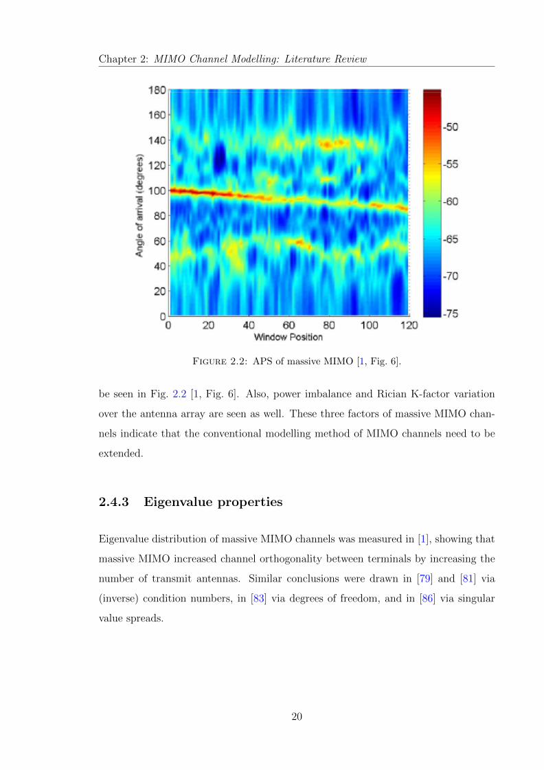
Figure 2.2: APS of massive MIMO [1, Fig. 6].
be seen in Fig. 2.2 [1, Fig. 6]. Also, power imbalance and Rician K-factor variation
over the antenna array are seen as well. These three factors of massive MIMO chan-
nels indicate that the conventional modelling method of MIMO channels need to be
extended.
2.4.3 Eigenvalue properties
Eigenvalue distribution of massive MIMO channels was measured in [1], showing that
massive MIMO increased channel orthogonality between terminals by increasing the
number of transmit antennas. Similar conclusions were drawn in [79] and [81] via
(inverse) condition numbers, in [83] via degrees of freedom, and in [86] via singular
value spreads.
20

Chapter 2: MIMO Channel Modelling: Literature Review
2.4.4 Other channel characteristics
Other channel characteristics such as angle Probability Density Function (PDF), Root
Mean Square (RMS) delay spread, Power Delay Profile (PDP), Angular Power Spec-
trum (APS) and correlation between subchannels were also studied in [79]–[94]. Au-
thor in [80] considered practical outdoor-to-indoor transmissions and observed that
there was hardly any extra capacity gain for more than 20 antennas when linear pre-
coding was applied. Furthermore, cell throughput and reflectivities of massive MIMO
with mmWave were measured in [96].
2.4.5 Challenges on massive MIMO channel measurements
For massive MIMO channels, it is important to measure parameters related to non-
stationary properties such as non-stationarities on the array axis as well as on the
time axis. However, these parameters are difficult to estimate since they fluctuate
from scenarios to scenarios. Hence, a large number of measurement campaigns are
required to capture those parameters.
Currently, many published measurement results were obtained via virtual antenna
arrays. To acquire more realistic channel characteristics, a large physical antenna
array is required. In this case, the mutual coupling effect between antenna elements
will be considered. However, from a realisation point of view, the increase of the
number of antennas will require many Radio Frequency (RF) chains and then raise
higher requirements for antenna calibrations.
Most of current measurements on massive MIMO channels focus on using ULAs.
However, to utilise space compactly, other types of arrays such as planar arrays and
cube arrays need to be considered.
21

Chapter 2: MIMO Channel Modelling: Literature Review
2.5 Research Gap
Channel measurements in Section 2.4 have shown that the above mentioned conven-
tional MIMO GBSMs in Section 2.2 are not suitable to be directly applied to modelling
massive MIMO channels. Measurements on massive MIMO channels in [1] and [87]
indicated that there are two characteristics making massive MIMO channels different
from conventional MIMO channels. First, since the number of antennas is huge in
massive MIMO systems, the farfield assumption in conventional MIMO channels may
no longer be appropriate. The distance between the receiver and transmitter (or a
cluster) may not be beyond the Rayleigh distance defined by 2L2
λ[97], where L and λ
are the dimension of the antenna array and carrier wavelength, respectively. For ULAs
with a fixed antenna separation ∆ (e.g., ∆ = λ/2), the dimension L = (M− 1) ∆
is linearly increasing with the number of antenna elements M. Therefore, the wave-
front should be assumed as spherical instead of plane when the number of antennas is
large. Although the impact of spherical wavefront on short-range or constant distance
communications was studied in [98] and [99], its impact on massive MIMO channels
has not yet been reported in the literature. Second, non-stationary properties can be
observed on large antenna arrays [1], i.e., appearance and disappearance of clusters
can occur on the array axis. This leads to the fact that each antenna element on
the array may observe different sets of clusters, which is not characterised in con-
ventional MIMO channels. As a result, the WSS assumption on antenna arrays does
not necessarily hold for massive MIMO channels. The authors in [100], [100]–[102]
modeled cluster evolution on the time axis with birth-death processes or Markov pro-
cesses. However, non-stationary properties of clusters on the array axis have not been
studied for massive MIMO channels in the literature.
Although GBSMs are able to capture the massive MIMO characteristic of cluster
evolution on the array axis mentioned in [1] and [87], they may not be feasible for
capacity analysis because of their complexity. CBSMs described in Section 2.3 cannot
fully characterise massive MIMO channel characteristics. Therefore, a novel simple
CBSM that considers different sets of scatterers for different antennas is necessary for
capacity analysis of massive MIMO channels.
22

Chapter 2: MIMO Channel Modelling: Literature Review
2.6 Summary
This chapter has reviewed and classified typical stochastic channel models for MIMO
channels, i.e., GBSMs, CBSMs. Features of each channel model have been introduced.
GBSMs are able to provide more accurate interpretations of realistic MIMO channels
at the cost of higher computational complexity. CBSMs are suitable for performance
analysis of MIMO systems for their simplicity. However, recent measurements of
massive MIMO channel characteristics have demonstrated that channel models for
conventional MIMO are insufficient for massive MIMO channels. Massive MIMO
channel models should take into account specific characteristics which differ them from
those in conventional MIMO channels, such as the spherical wavefront assumption
and non-stationary properties. This will normally increase the complexity of massive
MIMO channel models. First-order simplifications of the channel model will not be
appropriate with the spherical wavefront instead of plane wavefront assumption. Also,
conventional MIMO channel models cannot be directly applied to massive MIMO
channels in which different antennas may observe different sets of clusters. These two
important features are hardly to be embedded in CBSMs although they are simple.
On the other hand, complex GBSMs can reflect massive MIMO channel characteristics
but many more models for different practical scenarios are yet to be developed. 3-D
massive MIMO models, which jointly consider azimuth and elevation angles, are more
practical as well as complicated. In summary, new massive MIMO channel models
should be developed having a good tradeoff between model accuracy and complexity
and considering different practical scenarios with specific channel characteristics.
23

Chapter 3A Non-Stationary 2-D Ellipse Model for
Massive MIMO Channels
3.1 Introduction
A massive Multiple-Input Multiple-Output (MIMO) system is equipped with much
more antennas, typically tens or hundreds, than conventional MIMO systems [22],
[103]. With such a massive number of antennas, it has been demonstrated that a
massive MIMO system is able to provide many benefits, such as greatly increasing
the capacity, simplifying scheduling design in the frequency domain [22], and averaging
interference according to the large number theorem [23]. Generally speaking, a massive
MIMO system can be considered as an enhanced version of conventional MIMO by
utilizing an enormous number of antennas. As a result, its system performance, in
terms of capacity, efficiency, and reliability, is significantly better than conventional
MIMO systems [22], [103].
To design and evaluate MIMO systems, an accurate small-scale fading MIMO channel
model is necessary. Conventional small-scale fading MIMO channel models have been
widely studied in the literature. Extensive Geometry-Based Stochastic Models (GB-
SMs) for conventional MIMO channels known as one-ring model, two-ring model, and
ellipse model can be found in [34], [104]. Also, a combined ellipse and two-ring model
24

Chapter 3: A Non-Stationary 2-D Ellipse Model for Massive MIMO Channels
was proposed in [43] and [44], a multiple circular-ring model was proposed in [45], and
three-dimensional (3-D) concentric-cylinder models can be found in [56] and [105]. The
authors in [50] proposed a twin cluster model which concerned only the first and the
last bounces. The SCM [106], WINNER II model [30], IMT-A model [48], COST 273
model [52], and COST 2100 model [31], [33] have also been widely utilised. Besides,
correlation-based conventional MIMO channel models such as the Kronecker-Based
Stochastic Model (KBSM) and the Weichselberger model were used to investigate the
performance of massive MIMO systems in [107] and [70].
However, according to the measurement observations in [1] and [87], the above men-
tioned MIMO channel models [30], [31], [33], [34], [43]–[45], [48], [50], [52], [56], [70],
[104]–[107] are not sufficient to accurately capture certain characteristics of massive
MIMO channels. First, conventional MIMO channel models solely assume that the
distance between a scatterer and an antenna array is far beyond the Rayleigh dis-
tance [108], [109], i.e., 2L2/λ, where L is the dimension of the antenna array and λ
is the carrier wavelength. Namely, the farfield and plane wavefront assumptions were
usually applied to simplifying the channel models. However, the authors in [1] and [87]
stated that as the number of antennas is massive, the plane wavefront assumption is
not fulfilled for massive MIMO channels. Instead, a spherical wavefront channel model
should be considered. Spherical wavefront models and plane wavefront models were
compared in [110] and [99]. The authors in [110] pointed out that the plane wavefront
assumption underestimates the rank of the channel matrix. However, [110] and [99]
only focused on short range or constant distance communications which were not appli-
cable for general massive MIMO systems. Second, dynamic properties of clusters such
as cluster appearance and disappearance, Angle of Arrival (AoA) shifts, as well as non-
stationarities were observed on the antenna array axis [1], [87]. The characterisation
of non-stationarities was investigated in [100]–[102], [111], where the appearance and
disappearance of clusters on the time axis were modeled using the birth-death (BD)
or Markov processes. The authors in [61] and [112] analysed time-variant geometrical
properties such as AoA and Angle of Departure (AoD), but they ignored the evolu-
tion of clusters. However, [61], [100]–[102], [111], [112] only took non-stationarities
on the time axis into account and ignored non-stationarities on the array axis. The
25

Chapter 3: A Non-Stationary 2-D Ellipse Model for Massive MIMO Channels
authors in [113] considered nearfield effects and non-stationarities on the array axis.
However, in [113], the impact of spherical wavefront on Non-Line-of-Sight NLOS com-
ponents was missing, characteristics of cluster appearance and disappearance were not
studied in detail, and non-stationarities on the time axis were not included. A 3-D
non-stationary twin-cluster channel model was proposed in [51] for massive MIMO sys-
tems considering spherical wavefront and non-stationarities on both time and array
axes. However, AoAs and AoDs were assumed independent, channel characteristics
such as power imbalance on the antenn array and Space-Time-Frequency Correlation
Function (STFCF) were not investigated in [51].
In this chapter, a novel 2-D non-stationary wideband multi-confocal ellipse model
for massive MIMO systems is proposed. This channel model is developed aiming to
capture the spherical wavefront effect and non-stationary properties on both the array
and time axes. Also, AoAs and AoDs are assumed dependent in the ellipse model.
The major contributions of this chapter are summarised as follows:
1. The plane wavefront assumption for conventional MIMO channel models is re-
laxed, i.e., the nearfield effect of spherical wavefront is considered in the proposed
wideband ellipse model. The impacts of spherical wavefront assumption on both
the LOS component and NLOS components are studied.
2. Birth-Death (BD) process is applied to the array axis in order to capture the
cluster appearance and disappearance on the antenna array axis as reported in
[1]. Combining the BD process modelling cluster time evolution in [100], array-
time evolution of clusters of the proposed wideband massive MIMO channel
model is proposed. A novel cluster evolution algorithm is developed based on
the BD process on both the array and time axes.
3. Statistical properties of the proposed massive MIMO channel model such as
STFCF and Cumulative Distribution Functions (CDFs) of survival probabilities
of clusters and received power imbalance on the antenna array are investigated.
This chapter is organised as follows. In Section 3.2, the proposed wideband ellipse
MIMO channel model is discussed in detail. This includes geometrical properties
26

Chapter 3: A Non-Stationary 2-D Ellipse Model for Massive MIMO Channels
2f
O
nCluster
na21
2a
total2 Na
1Cluster
totalClusterN
T
lAnt
R
kAntT
ilnD,
T
inD ,R
inD ,
TET
in,D
LOS
lD
R
in,D REvD
v
Spherical wavefront
R
iknD,
LOS
lD
LOS
klD
Observable link
Non-observable link
R
pAnt
... ... ...
x
Figure 3.1: A wideband multi-confocal ellipse model for massive MIMO systems.
derived under the spherical wavefront assumption as well as the novel algorithm which
describes the cluster evolution on the array axis. Section 3.3 presents the array-time
evolution model, which describes dynamic properties of clusters on both the array and
time axes. Statistical properties are investigated as well. A corresponding wideband
ellipse simulation model is discussed in Section 3.4. In Section 3.5, numerical analysis
is given. Conclusions are finally drawn in Section 3.6.
3.2 A Wideband Ellipse Model for Massive MIMO
Systems
In this section, a novel wideband ellipse 2-D channel model for massive MIMO is
proposed, including spherical wavefront and cluster evolution on the array axis as
shown in Fig. 3.1. (The combination of cluster evolutions on both the time and array
27

Chapter 3: A Non-Stationary 2-D Ellipse Model for Massive MIMO Channels
axes will be presented in Section 3.3). Let us assume that the transmitter and receiver
are equipped with Uniform Linear Arrays (ULAs) with MT and MR omnidirectional
antennas, respectively. The antenna elements are spaced with separation δT and δR,
and they are located at the focal points of the confocal ellipses with a distance of
2f . One advantage of GBSMs is that the calculations of channel coefficients depend
only on geometry relationships between objects in the model. As a result, although
co-located antennas are used in this chapter for presentation convenience, the same
modeling approach can be generalised to distributed antenna arrays.
Let AntTl represent the l-th antenna of the transmit array and AntRk represent the k-th
antenna of the receive array. The n-th cluster is on the n-th ellipse with major axis
2an. The angle βT (βR) denotes the tilt angle of the transmit (receive) antenna array.
The angle αv denotes the angle between the x-axis and the direction of movement of
the receiver. The maximum Doppler frequency and carrier wavelength are denoted as
fmax and λ, respectively.
For massive MIMO channel models, there are two important properties should be
noticed. First, the farfield assumption for conventional MIMO channel models [34],
[43], which is equivalent to the plane wavefront assumption, is not fulfilled as the
dimension of the antenna array can not be ignored when the number of antennas is
massive. As a result, the wavefront emitted from the n-th cluster to the receive array
is assumed to be spherical as shown in Fig. 3.1. Then, the AoA is no longer linear
along the array, and it needs to be computed based on geometrical relationships. The
impact of spherical wavefront will be analysed in detail in following paragraphs.
Second, as reported in [1] and [87], the behavior of clusters is not stationary on
the array axis, which means that a cluster may not always be observable to all the
antenna elements of an array in conventional MIMO channel models. An example
is given in Fig. 3.1 that Cluster1 is observable to AntTl but it is not observable to
AntRk . ClusterNtotalis observable to AntRk but it is non-observable to AntTl . Conversely,
Clustern is observable to both AntRk and AntTl but not to AntRp . These situations imply
that different antenna elements may observe different sets of clusters, which is not
assumed in conventional MIMO channel models. Let CTl (CR
k ) denote the cluster set
28

Chapter 3: A Non-Stationary 2-D Ellipse Model for Massive MIMO Channels
in which clusters are observable to AntTl (AntRk ), the generation of CTl and CR
k will
be modeled as BD processes as described in Section 3.2.1. Also, let Ntotal denote the
total number of clusters which are observable to at least one transmit antenna and
one receive antenna, Ntotal can be expressed as [51]
Ntotal = card
(MT⋃l=1
MR⋃k=1
(CTl (t)
⋂CRk (t)
))(3.1)
where the operator card(·) denotes the cardinality of a set. Then, a cluster, say
Clustern (n 6 Ntotal), is observable to both AntTl and AntRk if and only if Clustern ∈CTl ∩ CR
k
.
Table 3.1: Summary of key parameter definitions for the 2-D ellipse model.
δT (δR) antenna spacing of the transmit (receive) antenna arrayMT (MR) number of transmit (receive) antennas
2f distance between the transmitter and receiver (focal length)an semi-major axis of the n-th ellipse
βT (βR) tilt angles of the transmit (receive) antenna arrayfmax, λ maximum Doppler frequency and carrier wavelength
AntTl , AntRk the l-th transmit antenna and the k-th receive antenna
DLOSkl LOS distance between AntRk and AntTl
DTln,i distance between the n-th cluster and AntTl via the i-th ray within the cluster
DRkn,i distance between the n-th cluster and AntRk via the i-th ray within the cluster
fLOSkl Doppler frequency of the LOS component between AntRk and AntTlfn,i Doppler frequency of the n-cluster via the i-th ray
ϕLOSkl phase of the LOS component between AntRk and AntTl
ϕkl,n,i phase of the n-th cluster between AntRk and AntTl via the i-th rayαTn,i AoD of the i-th ray of the n-th cluster to the transmit array center
αRn,i AoA of the i-th ray of the n-th cluster to the receive array center
Based on the above mentioned analysis and the summary of key parameter definitions
in Table 3.1, the wideband massive MIMO channel can be presented as an MR ×
MT complex matrix H(t, τ) = [hkl(t, τ)]MR×MT, where k = 1, 2, · · · ,MR and l =
1, 2, · · · ,MT . Next, assume the initial phase of the signal at the transmitter is ϕ0,
LOS Rician factor is K and the LOS component is always connected to all antennas
and the first cluster to arrive at the receiver if the LOS component exists. Additionally,
assume that the mean power of the n-th cluster is Pn and there are S rays within
one cluster and αRn,i is the AoA of the i-th ray of the n-th cluster to the receive array
center, αTn,i is the AoD of the i-th ray of the n-th cluster (i = 1, 2, · · · , S) to the
29

Chapter 3: A Non-Stationary 2-D Ellipse Model for Massive MIMO Channels
transmit array center, the multipath complex gains hkl(t, τ) of the theoretical model
(S →∞) between AntTl and AntRk at delay τ can be presented as
hkl(t, τ) =
Ntotal∑n=1
hkl,n(t)δ(τ − τn) (3.2)
where the complex gain hkl,n(t) of Clustern can be computed as
-if Clustern ∈CTl ∩ CR
k
,
hkl,n(t) = δ(n− 1)
√K
K + 1ej(2πfLOS
kl t+ϕLOSkl )︸ ︷︷ ︸
LOS
+
√Pn
K + 1limS→∞
1√S
S∑i=1
ej(2πfn,it+ϕkl,n,i)
︸ ︷︷ ︸NLOS
(3.3)
-if Clustern /∈CTl ∩ CR
k
,
hkl,n(t) = 0. (3.4)
For the LOS component, under the spherical wavefront assumption,
ϕLOSkl = ϕ0 +
2π
λ[(DLOS
l )2 +
(MR − 2k + 1
2δR
)2
− (MR − 2k + 1)δRDLOSl cos(αLOS
l − βR)]1/2 (3.5)
where
DLOSl = [(2f)2 +
(MT − 2l + 1
2δT
)2
− 2f(MT − 2l + 1)δT cos(βT )]1/2 (3.6)
and the AoA αLOSl of the LOS component from AntTl to the receive array center can
be computed as
αLOSl = π − arcsin
[sin βTDLOSl
(MT − 2l + 1
2δT
)]. (3.7)
30

Chapter 3: A Non-Stationary 2-D Ellipse Model for Massive MIMO Channels
The Doppler frequency fLOSkl of the LOS component between AntRk and AntTl can be
calculated as
fLOSkl = fmax cos(π − arcsin
[DLOSl
DLOSkl
sin(αLOSl − βR)
]) (3.8)
where
DLOSkl = [(DLOS
l )2 +
(MR − 2k + 1
2δR
)2
− (MR − 2k + 1)δRDLOSl cos(αLOS
l − βR)]1/2.
(3.9)
For the NLOS components, AoAs αRn,i and AoDs αTn,i are dependent in an ellipse
model, their relationship can be presented as [34]
αTn,i =
g(αRn,i) if 0 < αRn,i 6 α0
g(αRn,i) + π if α0 < αRn,i 6 2π − α0
g(αRn,i) + 2π if 2π − α0 < αRn,i 6 2π
(3.10)
where
g(αRn,i) = arctan
[(k2
0 − 1) sin(αRn,i)
2k0 + (k20 + 1) cos(αRn,i)
](3.11)
α0 = π − arctan
(k2
0 − 1
2k0
)(3.12)
k0 = an/f. (3.13)
Given the semi-major axis a1 of the first ellipse, the semi-major axis (size) of the n-th
ellipse, i.e., an, can be determined by τn relative to the first ellipse as
an = cτn + a1 (3.14)
where c is the speed of light. Accordingly, the distance between the n-th cluster and
the transmitter via the i-th ray, DTn,i, as well as the distance between the n-th cluster
and the receiver via the i-th ray, DRn,i, can be derived according to their geometrical
31

Chapter 3: A Non-Stationary 2-D Ellipse Model for Massive MIMO Channels
relationships:
DRn,i =
2an sinαTn,isinαTn,i + sin(π − αRn,i)
(3.15)
DTn,i =
2an sin(π − αRn,i)sinαTn,i + sin(π − αRn,i)
. (3.16)
Then, the distance between the n-th cluster and AntTl via the i-th ray within the
cluster, DTln,i, can be computed as
DTln,i = [(DT
n,i)2 +
(MT − 2l + 1
2δT
)2
− (MT − 2l + 1)δTDTn,i cos(βT − αTn,i)]1/2.
(3.17)
The distance between the n-th cluster and AntRk via the i-th ray within the cluster,
DRkn,i, can be computed as
DRkn,i = [(DR
n,i)2 +
(MR − 2k + 1
2δR
)2
− (MR − 2k + 1)δRDRn,i cos(αRn,i − βR)]1/2.
(3.18)
Based on the above equations, the received phase of AntRk via the i-th ray within the
n-th cluster from AntTl , ϕkl,n,i, can be expressed as
ϕkl,n,i = ϕ0 +2π
λ
(DTln,i +DR
kn,i
). (3.19)
The Doppler frequency of the i-th ray within the n-th cluster, fn,i, is
fn,i = fmax cos(αRn,i − αv). (3.20)
3.2.1 Array axis evolution—generation of cluster sets CTl and
CRk
Thus far, all the geometrical relationships have been derived from (3.5) to (3.20). In
this section, we will model the dynamic properties of clusters, i.e., the appearance
and disappearance of clusters on the array axis, using a BD process. In previous
32

Chapter 3: A Non-Stationary 2-D Ellipse Model for Massive MIMO Channels
literature [100] and [114], the BD process was deployed to model the channel non-
stationarity along the time axis, describing the cluster variations in terms of the change
of time. For massive MIMO systems, the time axis BD process [100] will be adapted
to the array axis [51]. Let λG (per meter) and λR (per meter) denote the cluster
generation rate and the recombination rate. Next, by defining the scenario-dependent
correlation factor Dac on the array axis, let the operator
E→ represent evolution on
either array or time axis, when a cluster set evolves from AntTl−1 to AntTl or from
AntRk−1 to AntRk , denoted as CTl−1
E→ CTl or CR
k−1E→ CR
k , the survival probabilities
of the clusters inside the cluster set at the transmitter P Tsurvival and at the receiver
PRsurvival can be modeled as [115]
P Tsurvival = e
−λRδTDac (3.21)
PRsurvival = e
−λRδRDac . (3.22)
According to the BD process, the duration between two cluster appearances and the
duration between two cluster disappearances are exponentially distributed [111] [115],
the average number of newly generated clusters NTnew and NR
new based on the Poisson
process can be computed as [115]
E[NT
new
]=λGλR
(1− e−λR
δTDac
)(3.23)
E[NR
new
]=λGλR
(1− e−λR
δRDac
)(3.24)
where E[·] designates the expectation. Cluster sets of each antenna are generated
based on BD process on the array axis. The flowchart of the cluster generation
algorithm is shown in Fig. 3.2.
First, let the initial number of clusters be N , the initial cluster set of AntT1 be CT1 =
cT1 , cT2 , c
Tx , · · · , cTN
, and the initial cluster set of AntR1 be CR
1 =cR1 , c
R2 , c
Rx , · · · , cRN
,
where cTx and cRx denote cluster members of cluster sets of the transmitter and the
receiver, and the subscript x (x = 1, 2, · · · , N) of cTx and cRx denotes the cluster indices.
The cluster sets of the rest of antennas at the transmitter side CTl (l = 2, 3, · · · ,MT )
33

Chapter 3: A Non-Stationary 2-D Ellipse Model for Massive MIMO Channels
Initialize cluster set for transmit
antenna 1:
Initialize max cluster index at
transmitter side:
Clusters evolve from
to
Generate new clusters according
to the birth rate
No
Initialize cluster set for receive
antenna 1:
Initialize max cluster index at
receiver side:
Clusters evolve from
to
Generate new clusters according
to the birth rate
No
Randomly shuffle and pair clusters.
Eliminate unpaired clusters.
Generate cluster power,
delay and AoAs.
Yes Yes
TC1
)card( 1max
TTCI
?T
Ml !
T
lC 1
TTTNII newmaxmax
RC1
?R
Mk!
R
kC 1
TNnew
RNnew
T
lC
R
kC
2 l
)card( 1max
RRCI
2 k
RRRNII newmaxmax
1 ll 1 kk
Figure 3.2: Cluster generation algorithm flowchart.
and the receiver side CRk (k = 2, 3, · · · ,MR) can be generated from the evolution of
CT1 and CR
1 , respectively. The survival probability of clusters to the next antenna
is calculated according to (3.21) and (3.22). At the same time, new clusters are
generated based on Poisson process with mean numbers as (3.23) and (3.24). These
newly generated clusters are added to the cluster sets of corresponding antennas.
Since each cluster evolves gradually on the antenna array, i.e., it will not appear again
after its disappearance, antenna correlations have been naturally embedded in the
generation process.
Second, after obtaining cluster sets of each antenna,MT⋃l=1
CTl and
MR⋃k=1
CRk are the full
collections of clusters observable to the transmitter and receiver, respectively. To
mimic the arbitrariness of the propagation environment, the cluster indices inMT⋃l=1
CTl
andMR⋃k=1
CRk are shuffled and arranged in a random order. Then, cluster indices of the
transmitter and receiver are paired. This process determines to which transmit and
receive antennas each cluster is observable. An example of the random shuffling and
34

Chapter 3: A Non-Stationary 2-D Ellipse Model for Massive MIMO Channels
6 3 5 1 2 4
5 1 8 2 7 3 4 6
Transmitter cluster indices
Receiver cluster indices
Randomly shuffled and paired
Eliminated
Figure 3.3: An example of random shuffling and pairing between the transmitterand receiver cluster indices.
pairing process has been illustrated in Fig. 3.3. In this example, transmit antennas
who can observe cT6 share a common cluster with receiver antennas who can observe
cR5 . Other clusters can be determined in the same way. Meanwhile, it is possible that
the cardinalities ofMT⋃l=1
CTl and
MR⋃k=1
CRk are not equal, i.e., there are clusters that are
not observable to either the transmit array or the receive array. It can be seen in
Fig. 3.3 that two more clusters are observable to the receiver than the transmitter. In
this case, after random shuffling and pairing, two clusters are eliminated from the full
receiver cluster set. Then, the cluster indices of these remained clusters are reassigned
from 1 to Ntotal.
Last, the delays and mean power of clusters are generated according to the urban
macro-cell scenario in [30] where delays and mean power are drawn randomly obeying
the exponential distributions. After delays are obtained, the semi-major axes can be
determined via (3.14). Since mean power is related to delay in [30], the mean power of
a cluster is then related to the size of its corresponding ellipse. In addition, AoAs are
modeled as the von Mises distribution [116]. As von Mises distribution can be easily
adapted to other distributions such as uniform distribution and wrapped Gaussian
distribution, it is widely utilised in the literature [34], [43], [44] to model angular
dispersions.
35

Chapter 3: A Non-Stationary 2-D Ellipse Model for Massive MIMO Channels
3.2.2 Space Cross-Correlation Function (CCF) analysis
Regarding the analysis of the spatial properties of the wideband model for massive
MIMO with cluster evolution on the antenna arrays, the space CCF is introduced in
this section. The normalised space CCF ρkl,k′l′,n(δT , δR; t) between the link connecting
AntRk and AntTl and the link connecting AntRk′ and AntTl′ of the n-th cluster at time t
is defined as [34] [117]
ρkl,k′l′,n(δT , δR; t) = E
[hkl,n(t)h∗k′l′,n(t)
|hkl,n(t)||h∗k′l′,n(t)|
](3.25)
where h∗k′l′,n(t) denotes the conjugate of hk′l′,n(t). The LOS component and the NLOS
components are independent to each other. As a result, the space CCF can be rewrit-
ten as the sum of the spatial correlation of the LOS component ρLOSkl,k′l′,n(δT , δR; t) and
the spatial correlation of the NLOS components ρNLOSkl,k′l′,n(δT , δR; t).
ρkl,k′l′,n(δT , δR; t) = ρLOSkl,k′l′,n(δT , δR; t) + ρNLOS
kl,k′l′,n(δT , δR; t). (3.26)
For the spatial correlation of the LOS component,
ρLOSkl,k′l′,n(δT , δR; t) =
Kδ(n− 1)
K + 1ej(2πfLOS
kl t+ϕLOSkl −2πfLOS
k′l′ t−ϕLOSk′l′ ). (3.27)
For the spatial correlation of the NLOS components, a cluster observable to AntTl
and AntRk has a probability of e−λR|l−l′|δT /Dac e−λR|k−k
′|δR/Dac to survive to connect AntTl′
and AntRk′ . Since the number of rays is infinite in the theoretical model, the discrete
AoAs αRn,i can be represented by a continuous random variable αRn . Therefore, given
the Probability Density Function (PDF) of the AoA pαRn (αRn ), ρNLOSkl,k′l′,n(δT , δR; t) can
be computed as
ρNLOSkl,k′l′,n(δT , δR; t) =
eλR−|l−l′|δT−|k−k′|δR
Dac
Kδ(n− 1) + 1×∫ π
−πej[ϕkl,n(αRn )−ϕk′l′,n(αRn )]pαRn (αRn )dαRn .
(3.28)
36

Chapter 3: A Non-Stationary 2-D Ellipse Model for Massive MIMO Channels
Equations (3.27) and (3.28) indicate that the difference between ϕkl,n and ϕk′l′,n,
ϕkl,n − ϕk′l′,n does not only depend on the difference between subscripts l − l′ and
k−k′. This means the process on the array axis is not Wide Sense Stationary (WSS).
3.3 Array-Time Evolution Model
To describe the cluster evolution on both array and time axes, the proposed wideband
ellipse model is further improved by combining the BD process on the time axis
in [100]. As a result, an array-time evolution model is established. Additionally,
geometrical relationships among the transmitter, the receiver, and the clusters need
to be updated with time. An example of a cluster evolving on time axis is illustrated
in Fig. 3.4. Both clusters and the Mobile Station (MS) are moving. Clustern and the
receive antenna array move to new positions from t = tm to t = tm+1. Distances and
angle properties have to be updated based on geometrical relationships. It can be
seen that AoD, AoA, and transmission distance will be time-variant because of the
movement of the cluster and the terminal. Consequently, αTn , αRn , DTn , DR
n , DTln, DR
kn,
an, f , αv, and τn become time-variant as αTn (t), αRn (t), DTn (t), DR
n (t), DTln(t), DR
kn(t),
an(t), f(t), αv(t), and τn(t) correspondingly. Although there exists situations when
Base Station (BS), MS, and clusters are all moving, it should be noticed that those
situations can be equivalent to a static BS situation using the principles of relative
motion.
In this case, assume Clustern, (n = 1, 2, · · · , N) moves in an arbitrary direction ϕc,n
with a speed of vc at time instance t = tm (m = 1, 2, · · · ), then at t = tm+1, the
instant distance between two focal points f(tm+1) can be calculated as
2f(tm+1) = [[2f(tm)]2 + [v(tm+1 − tm)]2 + 4f(tm)v(tm+1 − tm) cos [αv(tm)]]1/2.
(3.29)
37

Chapter 3: A Non-Stationary 2-D Ellipse Model for Massive MIMO Channels
O
)(Cluster mn t
)(2 mn ta
)(Cluster 1mn t
T
lAnt
R
kAnt
)(2 mtf
)(2 1mtf
)(2 1mnta
vD
)( 1 mm ttv
nc,M)( 1 mmc ttv
)( m
T
n tD
)( 1m
T
n tD
)( m
R
n tD
)( 1m
R
n tD
)( m
T
n tD
1T
2T
)( 1m
T
n tD
)( 1m
R
n tD
)( 1m
T
ln tD
RE
TE
)( 1m
R
kn tD
x
;ÿ
Figure 3.4: Geometrical relationship evolution from t = tm to t = tm+1 of theellipse model.
Accordingly, the distance between the transmitter and Clustern, DTn (t), needs to be
updated at t = tm+1 as
DTn (tm+1) = [
[DTn (tm)
]2+ v2
c (tm+1 − tm)2 + 2DTn (tm)vc(tm+1 − tm) cos(αTn (tm)− ϕc,n)]1/2.
(3.30)
Referencing the instant ellipse of Clustern(tm+1), the instant AoD and the distance
between AntTl and Clustern, DTln(tm+1) can be obtained as
αTn (tm+1) = αTn (tm)− θ1 − θ2 (3.31)
θ1 = arcsin
[v(tm+1 − tm) sin(π − αv(tm))
2f(tm+1)
](3.32)
θ2 = arcsin
[vc,n(tm+1 − tm) sin(π − αTn (tm) + ϕc,n)
DTn (tm+1)
](3.33)
38

Chapter 3: A Non-Stationary 2-D Ellipse Model for Massive MIMO Channels
DTln(tm+1) = [DT
n (tm+1)2
+
(MT − 2l + 1
2δT
)2
−DTn (tm+1) (MT − 2l + 1) δT cos(βT − αTn (tm+1))]1/2. (3.34)
Similarly, the distance between the receiver and Clustern, DRn (t), the corresponding
instant delay τn(tm+1), and the instant movement direction αv(tm+1) of the receiver
are derived as
DRn (tm+1) = [[2f(tm+1)]2 +
[DTn (tm+1)
]2 − 4f(tm+1)DTn (tm+1) cos(αTn (tm+1))]1/2
(3.35)
2an(tm+1) = DTn (tm+1) +DR
n (tm+1) (3.36)
τn(tm+1) = τn(tm) +2an(tm+1)− 2an(tm)
c(3.37)
αv(tm+1) = αv(tm)− θ1. (3.38)
Next, according to the law of sines, the AoA of Clustern at t = tm+1, αRn (tm+1), the
distance between AntRk and Clustern, DRkn(tm+1), and Doppler frequency fn(αRn (tm+1))
are computed as
αRn (tm+1) = arcsin
[DTn (tm+1) sin[αTn (tm+1)]
DRn (tm+1)
](3.39)
DRkn(tm+1) = [DR
n (tm+1)2
+
(MR − 2k + 1
2δR
)2
−DRn (tm+1) (MR − 2k + 1) δR cos(αRn (tm+1)− βR + θ1)]1/2 (3.40)
fn(αRn (tm+1)) = fmax cos(αRn (tm+1)− αv(tm+1)). (3.41)
Besides geometrical relationships, cluster sets of each antenna evolve with time as
well. Thus, the time-variant CTl , CR
k , and Nnew are denoted as CTl (t), CR
k (t), and
Nnew(t), respectively. The evolution of clusters on the time axis is modeled as a
BD process [100]. Here, let CTl (tm) (l = 1, 2, · · · ,MT ;m = 0, 1, 2, · · · ) and CR
k (tm)
(k = 1, 2, · · · ,MR;m = 0, 1, 2, · · · ) denote the cluster set for AntTl and the cluster set
39

Chapter 3: A Non-Stationary 2-D Ellipse Model for Massive MIMO Channels
for AntRk at time instant tm. Then at the next time instant, each cluster member in
set(⋃MT
l=1 CTl (tm)
)⋃(⋃MR
k=1CRk (tm)
)evolves according to the BD process on the
time axis. A survived cluster member will remain in cluster sets. On the other hand, a
disappeared cluster member will be eliminated from all the cluster sets. Newly gener-
ated cluster members will be added to certain cluster sets according to the BD process
on the array axis. To sum up, the algorithm is based on two main operations, the
array-axis evolution and the time-axis evolution, an example is described as follows.
At the initial time instant t = tm, array-axis evolution will be first operated. As
Fig. 3.2 indicates, given CT1 (tm) and CR
1 (tm), the cluster set of AntTl is evolved from
the cluster set of AntTl−1, the cluster set of AntRk is evolved from the cluster set of
AntRk−1
CTl−1(tm)
E→ CTl (tm) 2 ≤ l ≤MT (3.42)
CRk−1(tm)
E→ CRk (tm) 2 ≤ k ≤MR. (3.43)
Then, at the next time instant t = tm+1, time-axis evolution is operated as proposed
in [100]
CTl (tm)
E→ CTl (tm+1) (3.44)
CRk (tm)
E→ CRk (tm+1). (3.45)
To perform the evolution process of clusters on the time axis as (3.44) and (3.45) show,
define channel fluctuation in time domain at t = tm+1 as qm+1. The channel fluctuation
is a measure of how much the scattering environment has changed. Assuming that
the receiver and clusters are moving with a constant velocity, qm+1 is defined as [100]
qm+1 = qx,m+1 + qt,m+1 (3.46)
where qx,m+1 is the fluctuation caused by the movement of receiver, which is defined
as the distance the receiver moved with the time interval [100]
qx,m+1 = v(tm+1 − tm) (3.47)
and qt,m+1 is the fluctuation caused by the movement of clusters (PF is the percentage
40

Chapter 3: A Non-Stationary 2-D Ellipse Model for Massive MIMO Channels
of moving clusters, vc is the velocity of clusters), which is defined as the distance the
cluster moved with the time interval [100]
qt,m+1 = PFvc(tm+1 − tm). (3.48)
Given the scenario-dependent correlation factor Dsc on the space axis, each cluster
survives with probability Psurvival, which can be calculated as [115]
Psurvival(qm+1) = e−λRqm+1
Dsc . (3.49)
New clusters are generated according the Poisson process. The mean number of newly
generated clusters at time instant t = tm+1 on the time axis E[Nnew(tm+1)] is presented
as [115]
E[Nnew(tm+1)] =λGλR
(1− e−λRqm+1
Dsc ). (3.50)
For survived clusters, their geometrical relationships are computed as from (3.29) to
(3.41). On the other hand, the delays, mean power of newly generated clusters are
randomly drawn according to [30], where delays and mean power are exponentially
distributed. The AoAs of newly generated clusters obey the von Mises distribution.
To decide which transmit (receive) antennas are able to observe a newly generated
cluster, the newly generated cluster is first attached to one transmit (receive) antenna
with a randomly drawn index, say the ν-th transmit (receive) antenna. Second, this
cluster evolves to both ends of the transmit (receive) antenna array, ν + 1 to MT and
ν − 1 to 1 (or ν + 1 to MR and ν − 1 to 1), based on the survival probabilities on
the array axis P Tsurvival (PR
survival). Third, this cluster is added to antenna cluster sets
if it survives on those corresponding antennas. Finally, all cluster sets CTl (tm+1) and
CRk (tm+1) have been updated before entering the next time instant.
Prior to the derivation of STFCF, the time-variant transfer function Hkl(ξ, t) of the
channel can be expressed as [34]
Hkl(ξ, t) =
∞∫−∞
hkl(t, τ)e−j2πξτdτ
41

Chapter 3: A Non-Stationary 2-D Ellipse Model for Massive MIMO Channels
=
∞∫−∞
Ntotal∑n=1
hkl,n(t)δ(τ − τn)e−j2πξτdτ
=
Ntotal∑n=1
hkl,n(t)e−j2πξτn (3.51)
where ξ is frequency. The normalised STFCF ρkl,k′l′(δT , δR,∆ξ,∆t; ξ, t) can be calcu-
lated as [34]
ρkl,k′l′(δT , δR,∆ξ,∆t; ξ, t) = E
[H∗kl(ξ, t)Hk′l′(ξ + ∆ξ, t+ ∆t)
|H∗kl(ξ, t)||Hk′l′(ξ + ∆ξ, t+ ∆t)|
]
= E
Ntotal∑m=1
Ntotal∑n=1
h∗kl,m(t)hk′l′,n(t+ ∆t)ej2πξτm−j2π(ξ+∆ξ)τn
|H∗kl(ξ, t)||Hk′l′(ξ + ∆ξ, t+ ∆t)|
.(3.52)
With the Uncorrelated Scattering (US) assumption, i.e., clusters are mutually inde-
pendent
E[h∗kl,m(t)hk′l′,n(t+ ∆t)
]= 0 (3.53)
for m 6= n, the STFCF in (3.52) reduces to
ρkl,k′l′(δT , δR,∆ξ,∆t; t) = E
Ntotal∑n=1
h∗kl,n(t)hk′l′,n(t+ ∆t)ej2π∆ξτn
|H∗kl(ξ, t)||Hk′l′(ξ + ∆ξ, t+ ∆t)|
=
Ntotal∑n=1
E
[h∗kl,n(t)hk′l′,n(t+ ∆t)ej2π∆ξτn
|H∗kl(ξ, t)||Hk′l′(ξ + ∆ξ, t+ ∆t)|
]
=
Ntotal∑n=1
wnρkl,k′l′,n(δT , δR,∆ξ,∆t; t) (3.54)
where wn are normalisation weights such thatNtotal∑n=1
wnρkl,k′l′,n(0, 0, 0, 0; t) = 1 and
the normalised STFCF for the n-th cluster ρkl,k′l′,n(δT , δR,∆ξ,∆t; t) is defined by
42
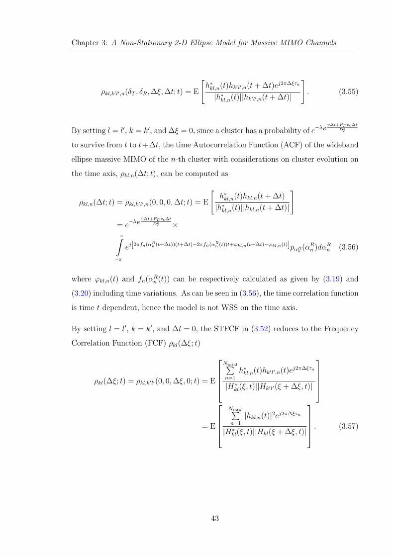
Chapter 3: A Non-Stationary 2-D Ellipse Model for Massive MIMO Channels
ρkl,k′l′,n(δT , δR,∆ξ,∆t; t) = E
[h∗kl,n(t)hk′l′,n(t+ ∆t)ej2π∆ξτn
|h∗kl,n(t)||hk′l′,n(t+ ∆t)|
]. (3.55)
By setting l = l′, k = k′, and ∆ξ = 0, since a cluster has a probability of e−λR
v∆t+PF vc∆t
Dsc
to survive from t to t+∆t, the time Autocorrelation Function (ACF) of the wideband
ellipse massive MIMO of the n-th cluster with considerations on cluster evolution on
the time axis, ρkl,n(∆t; t), can be computed as
ρkl,n(∆t; t) = ρkl,k′l′,n(0, 0, 0,∆t; t) = E
[h∗kl,n(t)hkl,n(t+ ∆t)
|h∗kl,n(t)||hkl,n(t+ ∆t)|
]= e
−λRv∆t+PF vc∆t
Dsc ×π∫
−π
ej[2πfn(αRn (t+∆t))(t+∆t)−2πfn(αRn (t))t+ϕkl,n(t+∆t)−ϕkl,n(t)]pαRn (αRn )dαRn (3.56)
where ϕkl,n(t) and fn(αRn (t)) can be respectively calculated as given by (3.19) and
(3.20) including time variations. As can be seen in (3.56), the time correlation function
is time t dependent, hence the model is not WSS on the time axis.
By setting l = l′, k = k′, and ∆t = 0, the STFCF in (3.52) reduces to the Frequency
Correlation Function (FCF) ρkl(∆ξ; t)
ρkl(∆ξ; t) = ρkl,k′l′(0, 0,∆ξ, 0; t) = E
Ntotal∑n=1
h∗kl,n(t)hk′l′,n(t)ej2π∆ξτn
|H∗kl(ξ, t)||Hk′l′(ξ + ∆ξ, t)|
= E
Ntotal∑n=1
|hkl,n(t)|2ej2π∆ξτn
|H∗kl(ξ, t)||Hkl(ξ + ∆ξ, t)|
. (3.57)
43

Chapter 3: A Non-Stationary 2-D Ellipse Model for Massive MIMO Channels
3.4 A Wideband Ellipse Simulation Model for Mas-
sive MIMO
The purpose of a simulation model is to obtain a reasonable trade-off between the
accuracy of the model and the complexity, i.e., approaching channel characteristics
(space CCF and time ACF) as precise as possible with a limited number of rays within
a cluster. As a result, in a NLOS scenario, (3.3) becomes
hkl,n(t) =
√PnS
S∑i=1
ej(2πfn,it+ϕkl,n,i). (3.58)
As fn,i and ϕkl,n,i are all functions of AoA, we need to find S rays with different AoAs
to achieve the simulation model. Given that AoAs obey the von Mises distribution
which can be characterised by its PDF [118]
pαRn (αRn ) =exp
[κ cos(αRn − αRn )
]2πI0(κ)
αRn ∈ [−π, π] (3.59)
where I0(·) is the zero-th order modified Bessel function, αRn is the mean and κ ≥
0 controls the width of the distribution. In the theoretical model, let g(αRn ) =h∗kl,n(t)hk′l′,n(t+∆t)
|h∗kl,n(t)||hk′l′,n(t+∆t)| with αRn distributed according to the von Mises distribution whose
PDF is as (3.59) shows. Furthermore, denote the CDF of the von Mises distribution
as F (αRn ). Then, the space-time correlation function equals The expectation of g(αRn )
which can be calculated as
ρkl,k′l′,n(δT , δR,∆t; t) = E[g(αRn )
]=
∫g(αRn )dF (αRn ). (3.60)
On the other hand, a simulation model aims at approximating ρkl,k′l′,n(δT , δR,∆t; t)
with S discrete AoAsαRn,iSi=1
. Each αRn,i follows the CDF F (αRn ). Then, the ap-
proximated value ρkl,k′l′,n(δT , δR,∆t; t) can be expressed as
ρkl,k′l′,n(δT , δR,∆t; t) =1
S
S∑i=1
g(αRn,i). (3.61)
44

Chapter 3: A Non-Stationary 2-D Ellipse Model for Massive MIMO Channels
The problem remains to determine theαRn,i
with reasonable computational complex-
ity to approximate ρkl,k′l′,n with ρkl,k′l′,n. With the Method of Equal Area (MEA) [34],
F (αRn ) is divided into S intervals with same probabilities, then αRn,i can be computed
as αRn,i = F−1( iS
), where F−1(·) is the inverse function of F (·). Although the CDF
and inverse CDF of the von Mises distribution is not analytic, αRn,i can be determined
numerically.
3.5 Numerical Analysis
In this section, numerical results of the proposed model will be analysed. To perform
numerical analysis, delays and mean power of clusters are assumed to be generated
according to the urban macro-cell scenario in [30] where both of them follow the
exponential distributions. AoAs of clusters to the receive array center are assumed to
be von Mises distributed.
The normalised Doppler Power Spectral Density (PSD) of the proposed model is
shown in Fig. 3.5. It should be noticed that the normalised Doppler PSD of the
proposed massive MIMO channel model is not symmetric with respect to 0, because
the decreasing correlation factor on temporal ACF resulting from cluster evolution
serves as a shift in the Fourier transform domain. Doppler PSD of simulations and
simulation models align well with the theoretical model, demonstrating the correctness
of derivations of the theoretical model.
The receiver absolute space CCF |ρk1,k′1,1(0, δR; t)| of the ellipse model under spherical
assumption in terms of different values of (k′, k) pairs with |k′ − k| = 1 is illustrated
in Fig. 3.6. It can be observed that the receive antenna correlation slowly decreases
as the normalised antenna spacing increases. The numerical results of the receive
antenna correlation curves of the proposed model are compared with measurement on
receiver correlation of massive MIMO in [1], showing that they share a similar trend.
It should be noted that the measurement on receiver correlation in [1] was obtained
via single experiment. Most importantly, it can be realised that correlation functions
of different values of k′ and k with |k′− k| = 1 are different. The correlation function
45

Chapter 3: A Non-Stationary 2-D Ellipse Model for Massive MIMO Channels
−500 −400 −300 −200 −100 0 100 200 300 400 5000
0.02
0.04
0.06
0.08
0.1
0.12
0.14
0.16
Doppler frequency (Hz)
Nor
mal
ized
PS
D
Theoretical model Simulation modelSimulation
Figure 3.5: Normalised Doppler PSD of the theoretical model, the simulationmodel, and simulations. (MR = 32,MT = 1, t = 1s, a1 = 100m, f = 80m,Dac = 30m, Ds
c = 50m, βR = βT = π/2, λ = 0.12m, fmax = 33.33Hz, αv = π/6,κ = 9, αRn = π/3, NLOS).
0 0.5 1 1.5 2 2.5
0.2
0.3
0.4
0.5
0.6
0.7
0.8
0.9
Normalized antenna spacing δR/λ
Receiver
absolute
space
CCF|ρ
k1,k′ 1,1(0,δ
R;t)|
Measurements
(k’,k)=(2,1)
(k’,k)=(8,7)
(k’,k)=(16,15)
(k’,k)=(32,31)
Figure 3.6: Absolute receiver space CCF |ρk1,k′1,1(0, δR; t)| of the ellipse modelunder von Mises assumption in terms of different values of (k′, k) pairs with |k′−k| =1. (MR = 32,MT = 1, t = 1s, a1 = 100m, f = 80m, Da
c = 30m, Dsc = 50m,
βR = βT = π/2, λ = 0.12m, fmax = 33.33Hz, αv = π/6, κ = 5, αRn = π/3, NLOS).
does not only depend of the absolute difference between antenna indices but also the
indices of reference antennas, which means the WSS properties on the antenna array
axis are not valid under the spherical wavefront assumption. The absolute space CCF
|ρ11,22,1(δT , δR; t)| of the ellipse model under spherical assumption has been illustrated
in Fig. 3.7. It can be observed that the spatial correlation gradually drops when the
normalised antenna spacing increases.
Furthermore, an example of cluster evolution on the array axis has been depicted
46

Chapter 3: A Non-Stationary 2-D Ellipse Model for Massive MIMO Channels
0
1
2
3
4
5 0
1
2
3
4
0
0.2
0.4
0.6
0.8
1
δT /λδR/λ
Absolute
space
CCF
|ρ11,22,1(δ
T,δ
R;t)|
Figure 3.7: Absolute space CCF |ρ11,22,1(δT , δR; t)| of the ellipse model. (MR =MT = 32, t = 1s, a1 = 100m, f = 80m, Da
c = 30m, Dsc = 50m, βR = βT = π/2,
λ = 0.15m, fmax = 33.33Hz, αv = π/6, κ = 5, NLOS).
in Fig. 3.8. Originally there are 20 clusters (Cluster1 to Cluster20) observable to
the first antenna element. Then, these clusters evolve according to the BD process
and probabilities described in Section 3.2.1. It can be observed that 4 (Cluster10,
Cluster14, Cluster15 and Cluster20) of the original 20 clusters disappear during the
evolutin process and 5 new clusters (Cluster21 to Cluster25) have been generated. As
a result, different antenna elements may observe different cluster sets. The cluster sets
of the 4th and the 31st receive antennas CR4 and CR
31, for instance, share 18 common
clusters. It should be noticed that, unlike conventional MIMO channel models, only
a total cluster number of a cluster set is not sufficient to represent the properties of
the cluster. The cluster members inside a cluster set as well as their properties such
as delay, AoA and cluster power should be considered when calculating the channel
coefficients in (3.3).
Fig. 3.9 and Fig. 3.10 show the normalised Angular Power Spectrum (APS) of AoA
of the wideband ellipse model for both NLOS and LOS scenarios. The value of λR is
set as 4/m, the values of λG are chosen as 80/m and 32/m for NLOS and LOS cases,
respectively. Hence, the mean numbers of clusters are aligned with NLOS (20 clusters)
and LOS (8 clusters) cases in the WINNER II model. The AoAs are estimated
using the well-known MUltiple SIgnal Classification (MUSIC) algorithm [119], [120]
with a sliding window formed by 3 consecutive antennas. This sliding window is
47
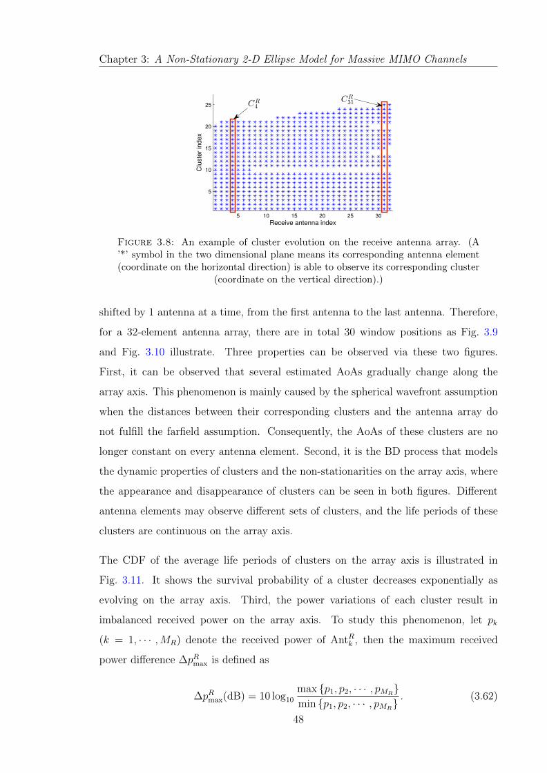
Chapter 3: A Non-Stationary 2-D Ellipse Model for Massive MIMO Channels
5 10 15 20 25 30
5
10
15
20
25
Receive antenna index
Clu
ste
r in
de
x
CR4
CR31
Figure 3.8: An example of cluster evolution on the receive antenna array. (A’*’ symbol in the two dimensional plane means its corresponding antenna element(coordinate on the horizontal direction) is able to observe its corresponding cluster
(coordinate on the vertical direction).)
shifted by 1 antenna at a time, from the first antenna to the last antenna. Therefore,
for a 32-element antenna array, there are in total 30 window positions as Fig. 3.9
and Fig. 3.10 illustrate. Three properties can be observed via these two figures.
First, it can be observed that several estimated AoAs gradually change along the
array axis. This phenomenon is mainly caused by the spherical wavefront assumption
when the distances between their corresponding clusters and the antenna array do
not fulfill the farfield assumption. Consequently, the AoAs of these clusters are no
longer constant on every antenna element. Second, it is the BD process that models
the dynamic properties of clusters and the non-stationarities on the array axis, where
the appearance and disappearance of clusters can be seen in both figures. Different
antenna elements may observe different sets of clusters, and the life periods of these
clusters are continuous on the array axis.
The CDF of the average life periods of clusters on the array axis is illustrated in
Fig. 3.11. It shows the survival probability of a cluster decreases exponentially as
evolving on the array axis. Third, the power variations of each cluster result in
imbalanced received power on the array axis. To study this phenomenon, let pk
(k = 1, · · · ,MR) denote the received power of AntRk , then the maximum received
power difference ∆pRmax is defined as
∆pRmax(dB) = 10 log10
max p1, p2, · · · , pMR
min p1, p2, · · · , pMR. (3.62)
48

Chapter 3: A Non-Stationary 2-D Ellipse Model for Massive MIMO Channels
Window position
An
gle
of
arr
iva
l (d
eg
ree
s)
5 10 15 20 25 30
0
20
40
60
80
100
120
140
160
180
1
0
Figure 3.9: A snapshot example of the normalised angle power spectrum of AoA ofthe wideband ellipse model. (MR = 32,MT = 1, a1 = 100m, f = 80m, Da
c = 30m,Dsc = 50m, βR = βT = π/2, λ = 0.15m, δR = 0.5λ, fmax = 0Hz, NLOS, λG = 80/m,
λR = 4/m, PF = 0.3).
Window position
An
gle
of
arr
iva
l (d
eg
ree
s)
5 10 15 20 25 30
0
20
40
60
80
100
120
140
160
180 0
1
Figure 3.10: A snapshot example of the normalised angle power spectrum ofAoA of the wideband ellipse model. (MR = 32,MT = 1, a1 = 100m, f = 80m,Dac = 30m, Ds
c = 50m, βR = βT = π/2, λ = 0.15m, δR = 0.5λ, fmax = 0Hz, LOSK = 3dB, λG = 32/m, λR = 4/m, PF = 0.3).
After 200 trials, the CDF of the the maximum received power difference in difference
conditions of correlation factors on array and space axes can be observed in Fig. 3.12.
It shows a difference of approximately 2− 3dB between the maximum and minimum
received power over the antenna array, which is normally not investigated in conven-
tional plane wavefront MIMO channel models. Also, the received power difference
on the array axis increases as the correlation factor reduces. Similar conclusions on
received power imbalance can be found in [1] and [87].
The absolute receiver space CCFs of the wideband ellipse model with different BD
49

Chapter 3: A Non-Stationary 2-D Ellipse Model for Massive MIMO Channels
0 50 100 150 200 2500
0.1
0.2
0.3
0.4
0.5
0.6
0.7
0.8
0.9
1
Average life periods on the array axis(normalized antenna spacing)
Pro
babili
ty
Theoretical (exponential distribution)
Simulated
Figure 3.11: Cumulative distribution function of average life periods of clusterson the array axis in terms of normalised antenna spacing. (Da
c = 30m, Dsc = 50m,
λ = 0.15m, δR = 0.5λ, NLOS, λG = 80/m, λR = 4/m, PF = 0.3).
0 1 2 3 4 5 6 7 8 9 100
0.1
0.2
0.3
0.4
0.5
0.6
0.7
0.8
0.9
1
Maximum received power difference (dB)
Pro
babili
ty
Da
c=D
s
c=50m, NLOS, mean=1.8dB
Da
c=D
s
c=30m, NLOS, mean=2.4dB
Da
c=D
s
c=50m, LOS K=3dB, mean=2.4dB
Da
c=D
s
c=30m, LOS K=3dB, mean=2.8dB
Figure 3.12: Cumulative distribution function of the maximum power differenceover the antenna array under different LOS/NLOS conditions and correlation factorson array and space axes. (MR = 32,MT = 1, a1 = 100m, f = 80m, βR = βT = π/2,
λ = 0.15m, δR = 0.5λ, fmax = 0Hz, von Mises distributed AoA).
process configurations is illustrated in Fig. 3.13. It can be observed that the correlation
with cluster evolution on the array axis is lower than that without considering array
evolution, because a certain number of clusters would fail to survive when they evolve
on the array axis. Also, the gap between the two curves increases as the antenna
separation grows because of a lower probability for a cluster to survive. Finally, the
time-variant characteristic has been shown in Fig. 3.14. It can be observed that the
absolute time ACF varies along with time and hence the numerical result demonstrates
time non-stationarities of the model.
50

Chapter 3: A Non-Stationary 2-D Ellipse Model for Massive MIMO Channels
0 1 2 3 4 5 6 7 8 9 100
0.1
0.2
0.3
0.4
0.5
0.6
0.7
0.8
0.9
1
Normalized antenna spacing δR/λ
Receiver
absolute
space
CCF
|ρ11,21,1(0,δ
R)|
with cluster evolution on the array axis
without cluster evolution on the array axis
Figure 3.13: Absolute receiver space CCF |ρ11,21,1(0, δR; t)| of the wideband ellipsemodel. (MR = 32,MT = 1, t = 1s, a1 = 100m, f = 80m, Da
c = 15m, Dsc = 50m,
βR = βT = π/2, λ = 0.15m, δR = 0.5λ, fmax = 0Hz, NLOS, λG = 80/m, λR = 4/m,PF = 0.3, κ = 5).
0 0.005 0.01 0.015 0.02 0.025 0.030
0.1
0.2
0.3
0.4
0.5
0.6
0.7
0.8
0.9
1
∆t(s)
Absolute
timeACF
|ρ11,1(∆
t;t)|
t=1s
t=4s
Figure 3.14: Absolute time ACF of Cluster1 |ρ11,1(∆t; t)| in (3.56) comparisonbetween t = 1s and t = 4s with BD process. (MR = 32,MT = 32, a1 = 100m,f = 80m, Da
c = 15m, Dsc = 50m, βR = βT = π/2, λ = 0.15m, δR = δT = 0.5λ,
fmax = 33.33Hz, vc = 0.5m/s, NLOS, λG = 80/m, λR = 4/m, PF = 0.3, κ = 5).
Fig. 3.15 compares the FCF between NLOS and LOS scenarios. It can be seen that
the FCF of NLOS decreases significantly with the frequency difference whose 50%
coherence bandwidth is approximately 1.2 MHz. On the other hand, the LOS scenario
has a larger 50% coherence bandwidth because the LOS component dominates the
power of the channel.
51

Chapter 3: A Non-Stationary 2-D Ellipse Model for Massive MIMO Channels
0 5 10 15 20 250
0.1
0.2
0.3
0.4
0.5
0.6
0.7
0.8
0.9
1
∆f (MHz)
Absolute
FCF
|ρ11(∆
f;t)|
NLOSLOS (K = 3dB)
Figure 3.15: Absolute FCF |ρ11(∆ξ; t)| comparison between NLOS and LOS.(MR = 32,MT = 32, a1 = 100m, f = 80m, Da
c = 15m, Dsc = 50m, βR = βT = π/2,
λ = 0.15m, δR = δT = 0.5λ, fmax = 33.33Hz, vc = 0.5m/s, λG = 80/m, λR = 4/m,PF = 0.3, κ = 5.)
3.6 Summary
A novel 2-D wideband ellipse channel model with non-stationarities on both time
and array axes for massive MIMO communication systems has been proposed in this
chapter. Spherical wavefront has been assumed in the proposed model illustrating
the difference of spatial correlation properties compared with the plane wavefront
assumption used in conventional MIMO channel models. It has been demonstrated
that WSS properties are not available under the spherical wavefront assumption.
Additionally, BD process has been applied to both time and array axes in order to
model the non-stationary behaviors of clusters on both axes. In this case, different
cluster sets can be observable to different antenna elements in this model. Finally,
based on the numerical analysis, the proposed model has shown that there are non-
stationarities and dynamic properties of clusters on the antenna array in massive
MIMO channels, where similar conclusions have also been drawn in measurements [1]
and [87]. For future work, certain parameters of the proposed channel model may be
extracted via measurements. Also, since GBSMs do not depend on configurations of
antenna arrays, polarised antenna arrays can be employed in future extensions of the
channel model.
52

Chapter 4A Non-Stationary 3-D Twin-Cluster Model
for Massive MIMO Channels
4.1 Introduction
In Chapter 3, a Two-Dimensional (2-D) Geometry-Based Stochastic Model (GBSM)
was proposed for massive Multiple-Input Multiple-Output (MIMO) channels. How-
ever, it was reported in [49] that scatterers would disperse in elevation (or the ver-
tical plane) and the impact of elevation angles needed to be addressed in realistic
channel models. Therefore, Three-Dimensional (3-D) channel models should be de-
veloped for massive MIMO systems. Extensive conventional 3-D MIMO models can
be found in the literature such as the twin-cluster MIMO model [50], the COST 2100
model [31], [33], 3-D extension of the WINNER model [60], 3-D double-directional
radio model [58], and 3-D MIMO Vehicle-to-Vehicle (V2V) channel model [56]. In
this chapter, we will extend the twin-cluster MIMO model in [50], where a cluster was
divided into two representations of itself (one at the transmitter and the other at the
receiver), by incorporating the spherical wavefront assumption, cluster evolution on
the time and array axes, and 3-D cluster properties to capture massive MIMO channel
characteristics.
The contributions of this chapter are summarised as follows:
53

Chapter 4: A Non-Stationary 3-D Twin-Cluster Model for Massive MIMO Channels
1. This chapter first proposes a theoretical non-stationary 3-D wideband twin-
cluster channel model for massive MIMO systems with carrier frequencies in
the order of gigahertz (GHz), i.e., they are not applicable to millimeter wave
communication systems. To the best of the authors’ knowledge, this is the first
3-D model for massive MIMO channels. An infinite number of scatterers is as-
sumed in the proposed theoretical model (or reference model), which cannot be
implemented in hardware or for simulation purposes. Therefore, we also propose
a corresponding 3-D simulation model with finite numbers of scatterers. Vari-
ous statistical properties, such as the Space-Time Correlation Function (STCF),
Doppler Power Spectral Density (PSD), and condition number, are studied for
both the theoretical and simulation models. Numerical results have demon-
strated that the statistical properties of the simulation model can fit those of
the theoretical model very well with reasonable complexity. Also, the impact of
cluster elevation angles on correlation properties of the proposed massive MIMO
channel models is investigated.
2. In the proposed theoretical and simulation massive MIMO channel models,
nearfield effects caused by the increasing antenna elements are considered, in-
cluding the spherical wavefront assumption and the variation of Doppler fre-
quencies over the antenna array.
3. Also, appearance and disappearance of clusters (i.e., cluster evolution) on both
the array and time axes are jointly modeled by Birth-Death (BD) processes,
which make the proposed massive MIMO channel models essentially non-stationary.
The rest of this chapter is organised as follows. Section 4.2 gives a general description
of the proposed theoretical non-stationary 3-D wideband twin-cluster channel model
for massive MIMO systems. Statistical properties of the proposed theoretical model
are studied in Section 4.3. Section 4.4 presents the corresponding simulation model for
the theoretical model. Numerical results are presented in Section 4.5 and conclusions
are finally drawn in Section 4.6.
54

Chapter 4: A Non-Stationary 3-D Twin-Cluster Model for Massive MIMO Channels
4.2 A Theoretical Non-Stationary 3-D Wideband
Twin-Cluster Massive MIMO Channel Model
Let us consider a wideband massive MIMO system with multiple twin clusters in a
3-D space to describe different taps of the channel, as illustrated in Fig. 4.1. For
a twin-cluster channel model with Ntotal clusters, each cluster, say Clustern (n =
1, . . . , Ntotal), is made of a representation ClusterTn at the transmitter side denoting
the first bounce and a representation ClusterRn at the receiver side denoting the last
bounce. The propagation environment between these two representations is abstracted
as a virtual link [50].
Let us assume that the transmitter and receiver are equipped with Uniform Lin-
ear Arrays (ULAs) with MT and MR antenna elements, respectively. It should be
mentioned that the calculations of channel coefficients depend only on geometry rela-
tionships between objects in the model and are independent to the layout of antenna
arrays. Therefore, although co-located ULAs are used in this chapter for presentation
convenience, the same modeling approach can be generalised to distributed antenna
arrays or 2-D antenna arrays.
The distances between antenna elements are δT at the transmitter and δR at the
receiver. Let the transmitter be the origin of the 3-D space, the distance vector
between the transmitter and receiver is D = (D, 0, 0). Furthermore, both azimuth
and elevation angles in the 3-D space are considered for clusters, antenna arrays,
movement direction of clusters, and movement direction of antenna arrays as listed in
Table 4.1. It should be noticed that the farfield conditions (D >2M2
T δ2T
λ, D >
2M2Rδ
2R
λ)
for conventional MIMO channels are not assumed in the proposed model. Thus, the
wavefront of each wireless link is assumed to be spherical resulting in the fact that
the Angles of Arrival (AoAs) and Angles of Departure (AoDs) on the antenna arrays
are no longer equal for each antenna element and the phase of each antenna element
is determined by geometrical relationships.
Another important characteristic of massive MIMO channel models is the appearance
and disappearance of clusters on the antenna array as reported in [1]. Contrary to
55

Chapter 4: A Non-Stationary 3-D Twin-Cluster Model for Massive MIMO Channels
conventional MIMO channel models assuming that a cluster is always observable to
all the antennas on an antenna array, a cluster may only be observable to a subset of
antennas on an antenna array for massive MIMO. To put it another way, each antenna
has its own set of observable clusters. Examples are shown in Fig. 4.1. Clustern+1
is observable to the k-th but not observable to the q-th (1 6 k, q 6 MR) receive
antenna. Similarly, Clustern+2 is observable to the l-th but not observable to the p-th
(1 6 l, p 6MT ) transmit antenna. On the other hand, Clustern is observable to both
the l-th transmit antenna and the k-th receive anteanna. Denote CTl (t)(CR
k (t)) as
the cluster set in which clusters are observable to the l-th transmit antenna (the k-th
receive antenna) at time instant t. Let Ntotal be the total number of clusters that are
observable to at least one transmit antenna and one receive antenna. The value of
Ntotal can be calculated as
Ntotal = card
(MT⋃l=1
MR⋃k=1
(CTl (t)
⋂CRk (t)
)). (4.1)
where the operator card(·) denotes the cardinality of a set. Then, a cluster is ob-
servable to the l-th transmit antenna and the k-th receive antenna if and only if this
cluster is in the setCTl (t)
⋂CRk (t)
. Sets CT
l (t) and CRk (t) are generated based on
the cluster evolution (BD process) on both the time and array axes as described in
Section 4.2.2.
Table 4.1: Definitions of key geometry parameters for the 3-D twin-cluster model.
υRE , υTE elevation angles of the receive and transmit antenna arrays
υRA , υTA azimuth angles of the receive and transmit antenna arrays
ξRn,i1 , θRn,i1 elevation and azimuth angles of the i1-th ray of the n-th cluster at the receiver side
ξTn,i2 , θTn,i2 elevation and azimuth angles of the i2-th ray of the n-th cluster at the transmitter side
AntTl , AntRk the l-th transmit antenna and the k-th receive antenna
DRn (t), DT
n (t) distance vectors between the n-th cluster and the receiver (transmitter)
DRn,i1
(t) distance vector between the n-th cluster and the receive antenna array via the i1-th ray
DRkn,i1
(t) distance vector between the n-th cluster and AntRk via the i1-th ray
DTn,i2
(t) distance vector between the n-th cluster and the transmit antenna array via the i2-th ray
DTln,i2
(t) distance vector between the n-th cluster and AntTl via the i2-th ray
DLOSkl (t) distance vector between AntRk and AntTl
v velocity vector of the receive antenna array
vRn , vTn velocity vectors of the n-th cluster at the receiver and transmitter side
56
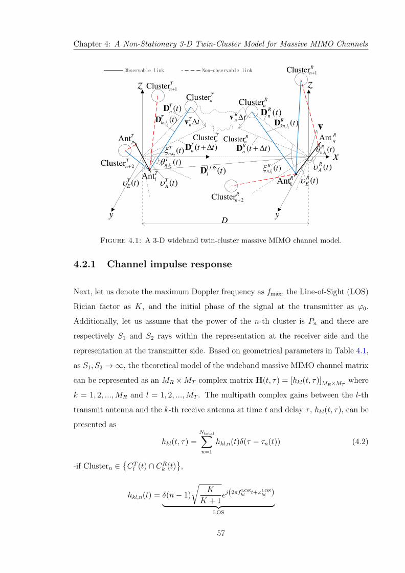
Chapter 4: A Non-Stationary 3-D Twin-Cluster Model for Massive MIMO Channels
T
nCluster
z
y
z
y
T
lAnt R
kAnt
)(1,t
R
inT
)(1,t
R
in[)(
2,t
T
inT
)(2,t
T
in[
R
nCluster
R
n 1Cluster
T
n 1Cluster
T
n 2Cluster
R
n 2Cluster
D
)(tR
nD
)(1,t
R
iknD)(
2,t
T
ilnD
)(tT
nD
)(LOS
tlD)(t
R
AX
)(tR
EX)(tT
AX)(tT
EX
v
Observable link Non-observable link
x
T
pAntR
qAnt
tT
n'v
T
nCluster
)( ttT
n 'D
R
nCluster
tR
n 'v
)( ttR
n 'D
Figure 4.1: A 3-D wideband twin-cluster massive MIMO channel model.
4.2.1 Channel impulse response
Next, let us denote the maximum Doppler frequency as fmax, the Line-of-Sight (LOS)
Rician factor as K, and the initial phase of the signal at the transmitter as ϕ0.
Additionally, let us assume that the power of the n-th cluster is Pn and there are
respectively S1 and S2 rays within the representation at the receiver side and the
representation at the transmitter side. Based on geometrical parameters in Table 4.1,
as S1, S2 →∞, the theoretical model of the wideband massive MIMO channel matrix
can be represented as an MR ×MT complex matrix H(t, τ) = [hkl(t, τ)]MR×MTwhere
k = 1, 2, ...,MR and l = 1, 2, ...,MT . The multipath complex gains between the l-th
transmit antenna and the k-th receive antenna at time t and delay τ , hkl(t, τ), can be
presented as
hkl(t, τ) =
Ntotal∑n=1
hkl,n(t)δ(τ − τn(t)) (4.2)
-if Clustern ∈CTl (t) ∩ CR
k (t)
,
hkl,n(t) = δ(n− 1)
√K
K + 1ej(2πfLOS
kl t+ϕLOSkl )︸ ︷︷ ︸
LOS
57

Chapter 4: A Non-Stationary 3-D Twin-Cluster Model for Massive MIMO Channels
+
√Pn
K + 1lim
S1,S2→∞
S1∑i1=1
S2∑i2=1
ej(2πfkn,i1 t+ϕkl,n,i1i2)√S1S2︸ ︷︷ ︸
NLOS
(4.3)
-if Clustern /∈CTl (t) ∩ CR
k (t)
,
hkl,n(t) = 0. (4.4)
The calculation of complex gains can be divided into Non-LOS (NLOS) components
and LOS component.
4.2.1.1 For NLOS components
The k-th receive antenna vector ARk (t) and the vector between the n-th cluster and
the receive antenna array via the i1-th ray DRn,i1
(t) can be presented as
ARk (t) =
MR − 2k + 1
2δR
cos υRE(t) cos υRA(t)
cos υRE(t) sin υRA(t)
sin υRE(t)
T
+ D (4.5)
DRn,i1
(t) = DRn (t)
cos ξRn,i1(t) cos θRn,i1(t)
cos ξRn,i1(t) sin θRn,i1(t)
sin ξRn,i1(t)
T
+ D. (4.6)
Similarly, the l-th transmit antenna vector ATl and the vector between the n-th cluster
and the transmit antenna array via the i2-th ray DTn,i2
(t) can be given as
ATl =
MT − 2l + 1
2δT
cos υTE cos υTA
cos υTE sin υTA
sin υTE
T
(4.7)
DTn,i2
(t) = DTn (t)
cos ξTn,i2(t) cos θTn,i2(t)
cos ξTn,i2(t) sin θTn,i2(t)
sin ξTn,i2(t)
T
. (4.8)
58

Chapter 4: A Non-Stationary 3-D Twin-Cluster Model for Massive MIMO Channels
Then, vectors DRkn,i1
(t) and DTln,i2
(t) can be computed as
DRkn,i1
(t) = DRn,i1
(t)−ARk (t) (4.9)
DTln,i2
(t) = DTn,i2
(t)−ATl . (4.10)
Next, the delay of the n-th cluster of the twin-cluster model is assumed to be the sum
of two components. The first component is calculated according to the geometrical
relationships between the antenna arrays and cluster locations. The second component
abstracts the delay of the virtual link between the twin clusters. Then, the delay of
the n-th cluster τn(t) can be computed as
τn(t) =‖DT
n (t)‖+ ‖DRn (t)‖
c+ τn(t) (4.11)
where the abstracted delay of the virtual link τn(t) is randomly drawn according to the
uniform distribution U(D/c, τmax), and τmax is the maximum delay (τmax = 1845 ns
for NLOS [30]). The operator ‖ · ‖ denotes the Euclidean norm, and c is the speed
of light. Then, the phase between the k-th receive antenna and the l-th transmit
antenna via the i1-th ray at the receiver, the i2-th ray at the transmitter, and the
n-th cluster, ϕkl,n,i1i2(t), is derived as
ϕkl,n,i1i2(t) = ϕ0 +2π
λ
[‖DR
kn,i1(t)‖+ ‖DT
ln,i2(t)‖+ cτn(t)
]. (4.12)
Accordingly, the Doppler frequency of the k-th receive antenna via the i1-th ray of
the n-th cluster fkn,i1(t) is presented as
fkn,i1(t) =fmax
⟨DRkn,i1
(t),v⟩
‖DRkn,i1
(t)‖‖v‖(4.13)
where 〈·, ·〉 represents the inner product.
59

Chapter 4: A Non-Stationary 3-D Twin-Cluster Model for Massive MIMO Channels
Generate initial
cluster set
Generate delays,
cluster powers, AoAs,
and AoDs for the
initial cluster set
Array-time
evolution of
clusters
Generate channel
impulse response
Figure 4.2: Algorithm flowchart of the generation of the channel impulse response.
4.2.1.2 For LOS component
In the same way, the Doppler frequency fLOSkl (t) and phase ϕLOS
kl (t) of the LOS com-
ponents can also be calculated as
DLOSkl (t) = AR
k (t)−ATl (4.14)
fLOSkl (t) =
fmax
⟨DLOSkl (t),v
⟩‖DLOS
kl (t)‖‖v‖(4.15)
ϕLOSkl (t) = ϕ0 +
2π
λ‖DLOS
kl (t)‖. (4.16)
The generation procedure of the channel impulse response consists of the generation
of the initial cluster set, generation of parameters (delays, cluster powers, AoAs, and
AoDs) for the initial cluster set, array-time evolution of clusters, and the generation
of channel impulse response, as presented in Fig. 4.2. This algorithm is a generalised
version of the WINNER channel model [30] by adding an extra block of array-time
evolution of clusters to capture massive MIMO channel characteristics. The block of
array-time evolution of clusters will be discussed in the next section.
4.2.2 Non-stationary properties
The non-stationary process of the proposed massive MIMO channel model is based
on the array-time evolution of clusters which can be characterised by two parts. The
first part is the generation of cluster sets CTl (t) and CR
k (t) for each antenna based on
BD process on both the time and array axes. This aims at modelling not only the
phenomena of cluster appearance and disappearance on antenna arrays of massive
MIMO, but also non-stationary behaviors of clusters on the time axis. The generation
60

Chapter 4: A Non-Stationary 3-D Twin-Cluster Model for Massive MIMO Channels
No
Yes
No Yes
i=1
Cluster set generation on the array axis
based on birth-death process for transmit
and receive antenna arrays:
),...,2,1(),(T
T
lMltC
Random shuffling and pairing clusters
),...,2,1(),(R
R
kMktC
Cluster evolution on the time axis based on
birth-death process
Clusteri newly
generated?
Update geometrical
relationships of
Clusteri
Randomly generate AoA/
AoD/power/delay for
Clusteri
i<Ntotal?i=i+1t=t+t,
Power normalization
Add Clusteri to cluster
sets based on birth-
death process on the
array axis
Figure 4.3: Algorithm flowchart of array-time evolution of the proposed 3-D twin-cluster model.
procedure is achieved by extending the concept of BD process on the time axis in
previous literature [100], [111] to the array axis as well. The outcome of the first
part determines the cluster set of each antenna. The second part is the updates of
geometrical relationships with respect to the movements of the receiver and clusters.
The outcome of the second part determines all parameters for each cluster. The
algorithm flowchart describing the array-time cluster evolution is depicted in Fig. 4.3.
Part 1: To describe the algorithm of the array-time cluster evolution, let us first
61

Chapter 4: A Non-Stationary 3-D Twin-Cluster Model for Massive MIMO Channels
denote λG (per meter) and λR (per meter) as the cluster generation rate and re-
combination rate. Assume the initial number of clusters N and the initial cluster
sets of the 1-st transmit and receive antennas CT1 =
cTx : x = 1, 2, · · · , N
and
CR1 =
cRx : x = 1, 2, · · · , N
at the initial time instant t are given, where cTx and
cRx are two representations of Clusterx. Then, these clusters in cluster sets CT1 and CR
1
evolve according to BD process on the array axis to recursively generate the cluster
sets of the rest of antennas at the transmitter and receiver at the initial time instant
t, which is expressed as
CTl−1(t)
E→ CTl (t) (l = 2, 3, · · · ,MT ) (4.17)
CRk−1(t)
E→ CRk (t) (k = 2, 3, · · · ,MR) (4.18)
where the operatorE→ denotes cluster evolution on either the array or time axis. The
survival probabilities of the clusters inside the cluster set the on array axis at the
transmitter P Tsurvival and the receiver PR
survival can be modeled as exponential functions
[115]
P Tsurvival = e
−λRδTDac (4.19)
PRsurvival = e
−λRδRDac (4.20)
where Dac is the scenario-dependent correlation factor on the array axis. According
to the BD process, the average number of newly generated clusters NTnew and NR
new on
the array axis based on the BD process can be computed as [115]
E[NT
new
]=λGλR
(1− e−λR
δTDac
)(4.21)
E[NR
new
]=λGλR
(1− e−λR
δRDac
)(4.22)
where E[·] designates the expectation. After this process on the array axis, a number
of initial clusters may not survive for certain antennas. Meanwhile, new clusters may
appear on the array. Each cluster evolves gradually on the antenna array. It can
be observed from (4.19) to (4.22) that, if two antenna elements are more separated,
the probability that they share the same set of clusters is smaller. To imitate the
62
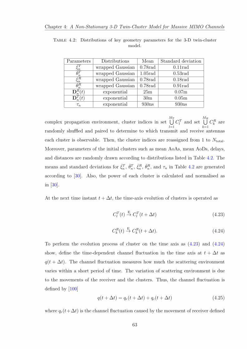
Chapter 4: A Non-Stationary 3-D Twin-Cluster Model for Massive MIMO Channels
Table 4.2: Distributions of key geometry parameters for the 3-D twin-clustermodel.
Parameters Distributions Mean Standard deviationξTn wrapped Gaussian 0.78rad 0.11radθTn wrapped Gaussian 1.05rad 0.53radξRn wrapped Gaussian 0.78rad 0.18radθRn wrapped Gaussian 0.78rad 0.91rad
DRn (t) exponential 25m 0.07m
DTn (t) exponential 30m 0.05mτn exponential 930ns 930ns
complex propagation environment, cluster indices in setMT⋃l=1
CTl and set
MR⋃k=1
CRk are
randomly shuffled and paired to determine to which transmit and receive antennas
each cluster is observable. Then, the cluster indices are reassigned from 1 to Ntotal.
Moreover, parameters of the initial clusters such as mean AoAs, mean AoDs, delays,
and distances are randomly drawn according to distributions listed in Table 4.2. The
means and standard deviations for ξTn , θTn , ξRn , θRn , and τn in Table 4.2 are generated
according to [30]. Also, the power of each cluster is calculated and normalised as
in [30].
At the next time instant t+ ∆t, the time-axis evolution of clusters is operated as
CTl (t)
E→ CTl (t+ ∆t) (4.23)
CRk (t)
E→ CRk (t+ ∆t). (4.24)
To perform the evolution process of cluster on the time axis as (4.23) and (4.24)
show, define the time-dependent channel fluctuation in the time axis at t + ∆t as
q(t + ∆t). The channel fluctuation measures how much the scattering environment
varies within a short period of time. The variation of scattering environment is due
to the movements of the receiver and the clusters. Thus, the channel fluctuation is
defined by [100]
q(t+ ∆t) = qr(t+ ∆t) + qc(t+ ∆t) (4.25)
where qr(t+∆t) is the channel fluctuation caused by the movement of receiver defined
63

Chapter 4: A Non-Stationary 3-D Twin-Cluster Model for Massive MIMO Channels
by qr(t + ∆t) = ||v||∆t and qc(t + ∆t) is the channel fluctuation caused by the
movement of clusters defined by qc(t+∆t) = PF (||vTn ||+||vRn ||)∆t (PF is the percentage
of moving clusters). Given the scenario-dependent space correlation factor Dsc , each
cluster survives with probability Psurvival on the time axis which can be calculated
as [100]
Psurvival(q(t+ ∆t)) = e−λRq(t+∆t)
Dsc . (4.26)
The mean number of newly generated clusters at time instant t+ ∆t on the time axis
E[Nnew(t+ ∆t)] is computed according to the BD process [115]
E[Nnew(t+ ∆t)] =λGλR
(1− e−λRq(t+∆t)
Dsc ). (4.27)
After the time evolution process as (4.23)-(4.27) show, all clusters can be categorised
as survived clusters or newly generated clusters. The next issue is to decide the set
of transmit and receive antennas that are observable to each newly generated cluster.
This is determined by the BD process on the array axis, which can be summarised
into 4 steps:
Step 1: Randomly generate initial indices l (1 6 l 6MT ) and k (1 6 k 6MR) for the
transmit and receive antenna arrays. Then, let the newly generated cluster
be observable to the l-th transmit antenna and the k-th receive antenna.
Step 2: Evolve the cluster on the transmit antenna array based on BD process from
the (l − 1)-th to the 1-st and from (l + 1)-th to the MT -th antennas.
Step 3: Evolve the cluster on the receive antenna array based on BD process from the
(k − 1)-th to the 1-st and from (k + 1)-th to the MR-th antennas.
Step 4: Add the cluster to cluster sets whose corresponding antennas can observe the
cluster.
Part 2: The remaining issue is the updates of geometry relationships of clusters from
t to t+ ∆t. The updates of geometry relationships are different for survived clusters
and newly generated clusters. Thus, they are described separately.
64

Chapter 4: A Non-Stationary 3-D Twin-Cluster Model for Massive MIMO Channels
4.2.2.1 Survived clusters
Regarding survived clusters, their properties such as delays, Doppler frequencies,
AoAs and AoDs should be recalculated based on the updates of geometrical rela-
tionships from t to t+ ∆t. First, the distance vectors are updated due to movements
of the receiver and clusters according to
DRn (t+ ∆t) = DR
n (t) + vRn∆t (4.28)
DTn (t+ ∆t) = DT
n (t) + vTn∆t (4.29)
DRkn,i1
(t+ ∆t) = DRn,i1
(t)−ARk (t) +
(vRn − v
)∆t (4.30)
DTln,i2
(t+ ∆t) = DTn,i2
(t) + vTn∆t−ATl . (4.31)
Second, the delay of the n-th cluster at t+ ∆t is expressed as the sum of the updated
geometrical delay and the delay of the evolved virtual link,
τn(t+ ∆t) =‖DT
n (t+ ∆t)‖+ ‖DRn (t+ ∆t)‖
c+ τn(t+ ∆t). (4.32)
To describe the evolution of the virtual link, its delay τn(t+∆t) is based on a first-order
filtering algorithm as τn(t+∆t) = e−∆tς τn(t)+(1−e−
∆tς )X where X is randomly drawn
according to the uniform distribution U(D/c, τmax), ς is a parameter that depends on
the coherence of a virtual link and scenarios. Third, the time-variant phase and
Doppler frequency are accordingly computed as
ϕkl,n,i1i2(t+ ∆t) = ϕ0 +2π
λcτn(t+ ∆t) +
2π
λ
[‖DR
kn,i1(t+ ∆t)‖+ ‖DT
ln,i2(t+ ∆t)‖
](4.33)
fkn,i1(t+ ∆t) =fmax
⟨DRkn,i1
(t+ ∆t),v⟩
‖DRkn,i1
(t+ ∆t)‖‖v‖. (4.34)
Last, geometrical relationships of LOS components need to be refreshed as well
DLOSkl (t+ ∆t) = AR
k (t) + v∆t−ATl (4.35)
65

Chapter 4: A Non-Stationary 3-D Twin-Cluster Model for Massive MIMO Channels
fLOSkl (t+ ∆t) =
fmax
⟨DLOSkl (t+ ∆t),v
⟩‖DLOS
kl (t+ ∆t)‖‖v‖(4.36)
ϕLOSkl (t+ ∆t) = ϕ0 +
2π
λ‖DLOS
kl (t+ ∆t)‖. (4.37)
4.2.2.2 Newly generated clusters
On the other hand, for newly generated clusters, their AoAs, AoDs, delays, and
distances are initialised according to distributions in Table 4.2. The power of each
cluster is calculated and normalised as in [30]. Denote the set of all survived clusters
as CSurvived and the set of all newly generated clusters as CNew after the time-axis
evolution. The average total power of survived and newly generated clusters should
be normalised as ∑Clusteri∈CSurvived
Pi +∑
Clusterj∈CNew
Pj = 1. (4.38)
Thus far, the array-time evolution of clusters from t to t+∆t is finished. This evolution
process can be operated recursively with respect to time.
4.3 Statistical Properties of the Theoretical Mas-
sive MIMO Channel Model
4.3.1 STCF
The STCF between the channel gains hkl,n(t) and hk′l′,n(t) is defined as [34]
ρkl,k′l′,n(δT , δR,∆t; t) = E
[h∗kl,n(t)hk′l′,n(t+ ∆t)
|h∗kl,n(t)||hk′l′,n(t+ ∆t)|
]. (4.39)
As the LOS component and NLOS components are independent, (4.39) can be rewrit-
ten as the sum of the STCFs of the LOS component and the NLOS components
ρkl,k′l′,n(δT , δR,∆t; t) = ρLOSkl,k′l′,n(δT , δR,∆t; t) + ρNLOS
kl,k′l′,n(δT , δR,∆t; t) (4.40)
66
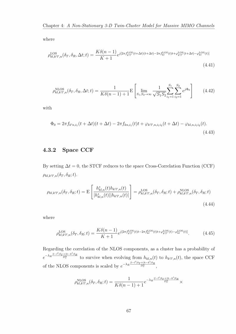
Chapter 4: A Non-Stationary 3-D Twin-Cluster Model for Massive MIMO Channels
where
ρLOSkl,k′l′,n(δT , δR,∆t; t) =
Kδ(n− 1)
K + 1ej[2πf
LOSk′l′ (t+∆t)(t+∆t)−2πfLOS
kl (t)t+ϕLOSk′l′ (t+∆t)−ϕLOS
kl (t)]
(4.41)
ρNLOSkl,k′l′,n(δT , δR,∆t; t) =
1
Kδ(n− 1) + 1E
[lim
S1,S2→∞
1√S1S2
S1∑i1=1
S2∑i2=1
ejΦ0
](4.42)
with
Φ0 = 2πfk′n,i1(t+ ∆t)(t+ ∆t)− 2πfkn,i1(t)t+ ϕk′l′,n,i1i2(t+ ∆t)− ϕkl,n,i1i2(t).
(4.43)
4.3.2 Space CCF
By setting ∆t = 0, the STCF reduces to the space Cross-Correlation Function (CCF)
ρkl,k′l′,n(δT , δR; t).
ρkl,k′l′,n(δT , δR; t) = E
[h∗kl,n(t)hk′l′,n(t)
|h∗kl,n(t)||hk′l′,n(t)|
]= ρLOS
kl,k′l′,n(δT , δR; t) + ρNLOSkl,k′l′,n(δT , δR; t)
(4.44)
where
ρLOSkl,k′l′,n(δT , δR; t) =
Kδ(n− 1)
K + 1ej[2πf
LOSk′l′ (t)t−2πfLOS
kl (t)t+ϕLOSk′l′ (t)−ϕLOS
kl (t)]. (4.45)
Regarding the correlation of the NLOS components, as a cluster has a probability of
e−λR
|l−l′|δT+|k−k′|δRDac to survive when evolving from hkl,n(t) to hk′l′,n(t), the space CCF
of the NLOS components is scaled by e−λR
|l−l′|δT+|k−k′|δRDac ,
ρNLOSkl,k′l′,n(δT , δR; t) =
1
Kδ(n− 1) + 1e−λR
|l−l′|δT+|k−k′|δRDac ×
67

Chapter 4: A Non-Stationary 3-D Twin-Cluster Model for Massive MIMO Channels
π∫−π
π∫−π
π2∫
−π2
π2∫
−π2
ejΦ1pR(ξRn , θRn )pT (ξTn , θ
Tn )dξRn dξ
Tn dθ
Rn dθ
Tn (4.46)
with
Φ1 = 2πfk′n(t)t− 2πfkn(t)t+ ϕk′l′,n(t)− ϕkl,n(t). (4.47)
As the space CCF ρkl,k′l′,n(δT , δR; t) depends on the values of k, k′, l, l′, and can not
be reduced to solely be with respect to |k− k′| and |l− l′|, the Wide Sense Stationary
(WSS) assumption on the array axis for massive MIMO is not valid.
4.3.3 Time ACF
On the other hand, by setting l = l′, k = k′, the time Autocorrelation Function (ACF)
ρkl,n(∆t; t) is obtained.
ρkl,n(∆t; t) = E
[h∗kl,n(t)hkl,n(t+ ∆t)
|h∗kl,n(t)||hkl,n(t+ ∆t)|
]= ρLOS
kl,n (∆t; t) + ρNLOSkl,n (∆t; t). (4.48)
Since the LOS component is uncorrelated to NLOS components, their time ACFs,
ρLOSkl,n (∆t; t) and ρNLOS
kl,n (∆t; t), are calculated separately as
ρLOSkl,n (∆t; t) =
Kδ(n− 1)
K + 1ej[2πf
LOSkl (t+∆t)(t+∆t)−2πfLOS
kl (t)t+ϕLOSkl (t+∆t)−ϕLOS
kl (t)]. (4.49)
Regarding the correlation of the NLOS components, the survival probability of a
cluster is e−λR
||v||∆t+PF (||vTn ||+||vRn ||)∆t
Dsc when evolving from hkl,n(t) to hkl,n(t + ∆t), the
time ACF of the NLOS components is scaled by e−λR
||v||∆t+PF (||vTn ||+||vRn ||)∆t
Dsc ,
ρNLOSkl,n (∆t; t) =
1
Kδ(n− 1) + 1e−λR
||v||∆t+PF (||vTn ||+||vRn ||)∆t
Dsc ×
π∫−π
π∫−π
π2∫
−π2
π2∫
−π2
ejΦ2pR(ξRn , θRn )pT (ξTn , θ
Tn )dξRn dξ
Tn dθ
Rn dθ
Tn (4.50)
68

Chapter 4: A Non-Stationary 3-D Twin-Cluster Model for Massive MIMO Channels
with
Φ2 = 2πfkn(t+ ∆t)(t+ ∆t)− 2πfkn(t)t+ ϕkl,n(t+ ∆t)− ϕkl,n(t). (4.51)
As the time ACF ρkl,n(∆t; t) depends on the values of t, and can not be reduced to
solely be with respect to ∆t, the WSS assumption on the time axis for the proposed
massive MIMO channel model is not valid.
4.3.4 Doppler PSD
The Doppler PSD Sn(f ; t) with respect to the Doppler frequency f is the Fourier
transform of the time ACF, which can be presented as
Sn(f ; t) :=
∫ ∞−∞
ρkl,n(∆t; t)e−j2πf∆td(∆t). (4.52)
It should be also noticed that the Doppler PSD is time dependent.
4.3.5 Doppler frequency standard deviation on the antenna
array
As spherical wavefronts are assumed in the proposed channel model, different an-
tennas on the same array will experience different Doppler shifts. Namely, Doppler
frequencies may vary on the antenna array. To study the variations of Doppler fre-
quency of the receiver on the array axis, the average Doppler frequency on the k-th
receive antenna, fkn, is calculated as
fkn =
π∫−π
π2∫
−π2
fkn(ξRn , θRn )p(ξRn , θ
Rn )dξRn dθ
Rn . (4.53)
Next, the average Doppler frequency on the array axis µfn is presented as µfn =
E[fkn]
=∑MRk=1 fknMR
. Finally, the standard deviation of Doppler frequency σfn on the
69

Chapter 4: A Non-Stationary 3-D Twin-Cluster Model for Massive MIMO Channels
array axis can be obtained as
σfn =
√∑MR
k=1
(fkn − µfn
)2
MR
. (4.54)
For conventional MIMO channel models, the Doppler frequency on the whole antenna
array is assumed to be the same which is equivalent to σfn = 0. Conversely, for
massive MIMO channel models, σfn may not be 0 and a larger σfn means that the
Doppler frequency varies more significantly on the antenna array.
4.3.6 Condition number
Condition number is used to measure the correlation of the channel matrix [22]. A
larger condition number implies higher correlation. The condition number is defined
by the quotient of maximum eigenvalue and the minimum eigenvalue of the channel
matrix
γ(dB) = 20 log10
λmax(H)
λmin(H)(4.55)
where the operators λmax(·) and λmin(·) represent the maximum eigenvalue and the
minimum eigenvalue, respectively.
4.4 A Non-Stationary 3-D Wideband Twin-Cluster
Simulation Model for Massive MIMO Chan-
nels
Previously, in the proposed channel theoretical model, the number of scatterers is
assumed to be infinity (S1, S2 → ∞) which is capable of providing accurate analytic
channel characteristic results. However, with respect to a channel simulator, infi-
nite scatterers are not practical as the complexity of implementation is enormous.
Therefore, a compromise between accuracy and complexity should be addressed. The
70

Chapter 4: A Non-Stationary 3-D Twin-Cluster Model for Massive MIMO Channels
target of this section is to develop a channel simulator with a finite and proper scat-
terer number while capturing channel characteristics as accurate as possible. The
corresponding simulation model of the proposed massive MIMO channel model is
obtained by reducing (4.3) as
hkl,n(t) = δ(n− 1)
√K
K + 1ej(2πfLOS
kl t+ϕLOSkl ) +
√Pn
K + 1
S1∑i1=1
S2∑i2=1
ej(2πfkn,i1 t+ϕkl,n,i1i2)√S1S2
.
(4.56)
Let x be the vector of AoAs and AoDs defined by x = (θR, ξR, θT , ξT ). In the
theoretical model, define g(x) =h∗kl,n(t)hk′l′,n(t+∆t)
|h∗kl,n(t)||hk′l′,n(t+∆t)| with x distributed according to
the Cumulative Distribution Function (CDF) F (x) of AoAs and AoDs. The STCF
ρkl,k′l′,n(δT , δR,∆t; t) for the theoretical model in (4.39) is calculated as the expectation
of g(x),
ρkl,k′l′,n(δT , δR,∆t; t) = E [g(x)] =
∫g(x)dF (x). (4.57)
On the other hand, a simulation model aims at approximating ρkl,k′l′,n(δT , δR,∆t; t)
with S1S2 discrete vectors xiS1S2
i=1 , where each xi follows the CDF F (x) and xi =
(θRi , ξRi , θ
Ti , ξ
Ti ). Then, the approximated value ρkl,k′l′,n(δT , δR,∆t; t) can be expressed
as
ρkl,k′l′,n(δT , δR,∆t; t) = E [g(x)] =1
S1S2
S1S2∑i=1
g(xi). (4.58)
The remaining issue is to determine the vector sequence xiS1S2
i=1 with reasonable com-
putational complexity to approximate ρkl,k′l′,n(δT , δR,∆t; t) with ρkl,k′l′,n(δT , δR,∆t; t).
A number of algorithms to calculate xiS1S2
i=1 such as the Method of Equal Distances
(MED), Method of Equal Area (MEA), Method of Exact Doppler Spread (MEDS),
and the Monte Carlo Method (MCM) have been introduced in [34]. Here, the MEA is
applied to calculating the discrete vectors xiS1S2
i=1 of the simulation model according
to∫ xi
xi−1dF (a) = 1
S1S2[34]. Since x is four dimensional in this model, the ‘area’ in
MEA in this case is generalised as the probability measure of a set. As a result, F (x)
is divided into S1S2 sets with the same probability of 1S1S2
, then xi can be computed
71

Chapter 4: A Non-Stationary 3-D Twin-Cluster Model for Massive MIMO Channels
as xi = F−1(
iS1S2
)where F−1(·) is the inverse function of F (·).
4.5 Numerical Results and Analysis
The distributions of azimuth and elevation angles at the transmitter side and the re-
ceiver side are assumed to obey the two dimensional von Mises distribution [118],
where azimuth angles and elevation angles are assumed to be mutually indepen-
dent. Therefore, the Probability Density function (PDF) of angles of the n-th cluster
pZ(ξZn , θZn ) with Z = T,R can be expressed as
pZ(ξZn , θZn ) =
exp[κ(cos(ξZn − ξZn ) + cos(θZn − θZn ))
][2πI0(κ)]2
(4.59)
where ξZn and θZn are the mean elevation and azimuth AoD/AoA, and I0(·) is the
zero-th order modified Bessel function. Moreover, κ > 0 controls the width of the
distribution functions.
By setting ∆t to 0, the absolute values of the space CCF |ρ11,22,1(δT , δR; t)| of the
three dimensional twin cluster model are illustrated in Fig. 4.4. A decreasing trend
can be observed as the normalised antenna spacings increase at both the transmitter
and receiver sides. The absolute values of space CCF drop smoothly when antenna
spacing at the transmitter side enlarges. Meanwhile, fluctuations can be seen as
antenna spacing at the receiver side increases. These fluctuations are caused by non-
stationary properties due to the movements of the receiver.
Next, by setting δT and ∆t to 0, the impact of cluster elevation angles at the receiver
side on the absolute space CCF |ρ11,12,1(0, δR; t)| of the receiver is depicted in Fig. 4.5.
The increase in cluster elevation angles at the receiver side results in high receive
antenna correlations, because the projected distance of two antenna element in the
3-D space is proportional to the product of the cosine of the azimuth angle and the
cosine of the elevation angle. When the elevation angle increases from 0 to π/2, its
cosine value decreases. Besides, the space CCF of the simulation model is compared
with the theoretical model, showing that the simulation model is able to capture the
72
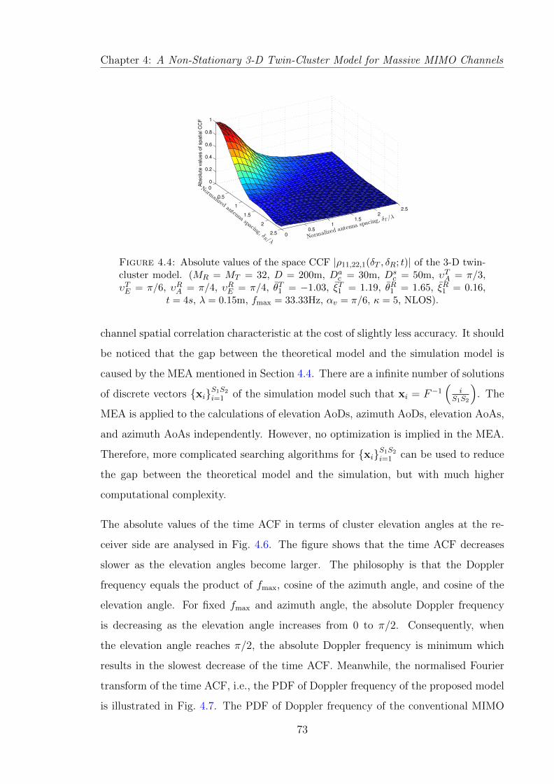
Chapter 4: A Non-Stationary 3-D Twin-Cluster Model for Massive MIMO Channels
0
0.5
1
1.5
2
2.5 00.5
11.5
22.5
0
0.2
0.4
0.6
0.8
1
Normalize
d antenna spaci
ng, δT/λ
Norm
alizedantenna
spacing, δR /λ
Absolu
te v
alu
es o
f spatial C
CF
Figure 4.4: Absolute values of the space CCF |ρ11,22,1(δT , δR; t)| of the 3-D twin-cluster model. (MR = MT = 32, D = 200m, Da
c = 30m, Dsc = 50m, υTA = π/3,
υTE = π/6, υRA = π/4, υRE = π/4, θT1 = −1.03, ξT1 = 1.19, θR1 = 1.65, ξR1 = 0.16,t = 4s, λ = 0.15m, fmax = 33.33Hz, αv = π/6, κ = 5, NLOS).
channel spatial correlation characteristic at the cost of slightly less accuracy. It should
be noticed that the gap between the theoretical model and the simulation model is
caused by the MEA mentioned in Section 4.4. There are a infinite number of solutions
of discrete vectors xiS1S2
i=1 of the simulation model such that xi = F−1(
iS1S2
). The
MEA is applied to the calculations of elevation AoDs, azimuth AoDs, elevation AoAs,
and azimuth AoAs independently. However, no optimization is implied in the MEA.
Therefore, more complicated searching algorithms for xiS1S2
i=1 can be used to reduce
the gap between the theoretical model and the simulation, but with much higher
computational complexity.
The absolute values of the time ACF in terms of cluster elevation angles at the re-
ceiver side are analysed in Fig. 4.6. The figure shows that the time ACF decreases
slower as the elevation angles become larger. The philosophy is that the Doppler
frequency equals the product of fmax, cosine of the azimuth angle, and cosine of the
elevation angle. For fixed fmax and azimuth angle, the absolute Doppler frequency
is decreasing as the elevation angle increases from 0 to π/2. Consequently, when
the elevation angle reaches π/2, the absolute Doppler frequency is minimum which
results in the slowest decrease of the time ACF. Meanwhile, the normalised Fourier
transform of the time ACF, i.e., the PDF of Doppler frequency of the proposed model
is illustrated in Fig. 4.7. The PDF of Doppler frequency of the conventional MIMO
73

Chapter 4: A Non-Stationary 3-D Twin-Cluster Model for Massive MIMO Channels
0 0.2 0.4 0.6 0.8 1 1.2 1.4 1.6 1.8 20
0.1
0.2
0.3
0.4
0.5
0.6
0.7
0.8
0.9
1
Normalized antenna spacing, δR/λ
Absolu
te v
alu
es o
f spatial C
CF
Theoretical modelSimulation model (S
1=S
2=81)
Cluster elevation angles
at the receiver side=
π/6,π/4,π/3
Figure 4.5: Absolute values of the receiver space CCF |ρ11,12,1(0, δR; t)| in termsof cluster elevation angles at the receiver side. (MR = 32, D = 200m, Da
c = 30m,Dsc = 50m, ς = 1s, υTA = π/3, υTE = π/6, υRA = π/4, υRE = π/4, θT1 = −1.03,
ξT1 = 1.19, θR1 = 1.65, t = 4s, λ = 0.15m, fmax = 33.33Hz, αv = π/6, κ = 5,NLOS).
channel model is symmetrical with respect to 0. However, this may not be necessary
for the proposed non-stationary massive MIMO channel model. There are two obser-
vations that should be noticed in Fig. 4.7. First, the PDFs of Doppler frequency at
different time instants vary because of the non-stationary properties on the time axis.
Namely, the WSS condition on the time domain is not available as a consequence of
time-variant properties and the inclusion of BD process on the time axis. The factor
e−λR
||v||∆t+PF (||vTn ||+||vRn ||)∆t
Dsc of the time ACF in (4.50) with respect to ∆t is equivalent
to a translation in the Fourier transform domain. Moreover, simulation models align
well with theoretical models as shown in Fig. 4.6 and Fig. 4.7.
In addition, Fig. 4.8 shows the standard deviation of Doppler frequencies on the
antenna array. Conventional MIMO channel models assume farfield condition which
results in a constant Doppler frequency on the entire antenna array. Conversely, the
nearfield condition is assumed in the proposed massive MIMO channel model. As a
result, the Doppler frequencies for different antennas are different. Since the nearfield
effect is more significant as the number of antennas grows, the standard deviation
increases accordingly.
Furthermore, a comparison of condition numbers between the 2-D and 3-D models is
shown in Fig. 4.9. Stronger correlations are observed in the 2-D model than the 3-D
74

Chapter 4: A Non-Stationary 3-D Twin-Cluster Model for Massive MIMO Channels
0 0.05 0.1 0.15 0.2 0.250
0.1
0.2
0.3
0.4
0.5
0.6
0.7
0.8
0.9
1
Time difference, ∆t(s)
Absolu
te v
alu
es o
f te
mpora
l A
CF
Theoretical model Simulation model (S
1=S
2=81)
Cluster elevation anglesat the receiver side=π/6,π/3,π/2
Figure 4.6: Absolute values of the time ACF |ρ11,1(∆t; t)| in terms of clusterelevation angle at the receiver side (MR = 32, D = 200m, Da
c = 30m, Dsc = 50m,
ς = 1s, υTA = π/3, υTE = π/6, υRA = π/4, υRE = π/4, θT1 = −1.03, ξT1 = 1.19,θR1 = 1.65, t = 4s, λ = 0.15m, ||vTn || = ||vRn || = 0.25m/s, PF = 0.3, fmax = 33.33Hz,
αv = π/6, κ = 5, NLOS).
−100 −80 −60 −40 −20 0 20 40 60 80 1000
0.1
0.2
0.3
0.4
0.5
0.6
Doppler freqency (Hz)
Norm
aliz
ed D
opple
r P
SD
Theoretical model (t=4s)
Simulation model (t=4s,S1 = S2 = 81)
Theoretical model (t=2s)
Simulation model (t=2s,S1 = S2 = 81)
Conventional MIMO theoretical model
Figure 4.7: The normalised Doppler PSD at different time instants (MR = 32,D = 200m, Da
c = 30m, Dsc = 50m, ς = 1s, υTA = π/3, υTE = π/6, υRA = π/4,
υRE = π/4, θT1 = −1.03, ξT1 = 1.19, θR1 = 1.65, λ = 0.15m, λG = 80/m, λR = 4/m,||vTn || = ||vRn || = 0.25m/s, PF = 0.3, fmax = 33.33Hz, αv = π/6, κ = 5, NLOS).
75

Chapter 4: A Non-Stationary 3-D Twin-Cluster Model for Massive MIMO Channels
10 20 30 40 50 60−0.5
0
0.5
1
1.5
2
2.5
3
3.5
Number of antennas
Sta
ndard
devia
tion o
f D
opple
r fr
equencie
s
on the a
nte
nna a
rray (
Hz)
Proposed massive MIMO model
Conventional MIMO model
Figure 4.8: Standard deviation of the Doppler frequencies on the antenna array(D = 200m, Da
c = 30m, Dsc = 50m, ς = 1s, υTA = π/3, υTE = π/6, υRA = π/4,
υRE = π/4, θT1 = −1.03, ξT1 = 1.19, θR1 = 1.65, ξR1 = 0.16, λ = 0.15m, ||vTn || =||vRn || = 0.25m/s, PF = 0.3, fmax = 33.33Hz, αv = π/6, κ = 5, NLOS).
15 20 25 30 35 40 450
0.1
0.2
0.3
0.4
0.5
0.6
0.7
0.8
0.9
1
Condition number (dB)
CD
F
2D model
3D model
Figure 4.9: Comparisons of CDFs of condition numbers between the 2-D and3-D model (MT = 4, MR = 32, D = 200m, Da
c = 30m, Dsc = 50m, ς = 1s,
υTA = π/3, υTE = π/6, υRA = π/4, υRE = π/4, θT1 = −1.03, ξT1 = 1.19, θR1 = 1.65,t = 4s, λ = 0.15m, λG = 80/m, λR = 4/m, ||vTn || = ||vRn || = 0.25m/s, PF = 0.3,
fmax = 33.33Hz, αv = π/6, κ = 5, NLOS).
model due to the fact that clusters have higher probabilities to be correlated in a 2-D
space than a 3-D space. However, this difference is relatively less significant because
the random distribution of cluster locations partially averages out the impact.
Fig. 4.10 illustrates the non-stationary properties on the array axis in the form of the
receiver Angular Power Spectrum (APS). It should be noticed that the estimated angle
here means the angle between the cluster and the receive antenna array. Here, the
MUltiple SIgnal Classification (MUSIC) algorithm [120] is applied to AoA estimation.
76

Chapter 4: A Non-Stationary 3-D Twin-Cluster Model for Massive MIMO Channels
Window position
An
gle
of
arr
iva
l (d
eg
ree
s)
5 10 15 20 25 30
20
40
60
80
100
120
140
160
180
1
0
Figure 4.10: A snap shot of the angular power spectrum of the receiver antennaarray (MT = 1, MR = 32, D = 200m, Da
c = 30m, Dsc = 50m, ς = 1s, υTA = π/3,
υTE = π/6, υRA = π/4, υRE = π/4, θT1 = −1.03, ξT1 = 1.19, θR1 = 1.65, t = 4s,λ = 0.15m, λG = 80/m, λR = 4/m, fmax = 0Hz, NLOS).
A sliding window formed by 3 consecutive receive antennas is shifted by 1 antenna
at a time from the first to the last antenna. Consequently, for a 32-element antenna
array, there are in total 30 window positions as Fig. 4.10 shows. Clusters appear
and disappear on the array axis, which results in that different antennas may observe
different sets of clusters. Additionally, angles of a number of clusters shift on the array
axis due to the nearfield effect. Finally, receive power variations can be observed on
the antenna array. Similar conclusions on these mentioned features of the proposed
model were also observed in measurements in massive MIMO channels in [1].
Regarding cluster evolution on the time axis, an example of cluster sets in different
time instants is shown in Fig. 4.11. Clusters evolve according to the BD process.
Thus, it can be seen that there are clusters disappearing and new clusters appearing.
In this case, the transmit and receive antenna arrays observe a time-variant set of
clusters.
It is important to note that in the numerical analysis, parameters such as mean and
standard deviation of azimuth AoAs/AoDs of the transmitter and receiver, mean
and standard deviation of delays, maximum delay, spatial correlation distance, and
cluster powers were generated according to the WINNER II channel model in [30]. The
generation and recombination rates of clusters and percentage of moving clusters were
adapted from [100] and [111]. However, certain parameters such as cluster distances
77

Chapter 4: A Non-Stationary 3-D Twin-Cluster Model for Massive MIMO Channels
0 2 4 6 8 10 120
5
10
15
20
25
30
Time, t (s)
Clu
ste
r in
dex
Figure 4.11: Cluster evolution on the time axis (Dsc = 50m, ς = 1s, λ = 0.15m,
λG = 80/m, λR = 4/m, ||vTn || = ||vRn || = 0.25m/s, PF = 0.3, fmax = 33.33Hz,NLOS).
to the transmitter or receiver were given based on reasonable assumptions, since we
have not found any relevant measurement data so far. These parameters of the model
can be further validated by measurements whenever available in the future.
4.6 Summary
Key characteristics of massive MIMO channels have not been captured by conven-
tional MIMO channel models. In this chapter, we have proposed a novel theoretical
non-stationary 3-D wideband twin-cluster channel model along with the correspond-
ing simulation model for massive MIMO systems with carrier frequencies in the order
of GHz. Spherical wavefronts have been assumed to characterise nearfield effects re-
sulting in AoA shifts, received power variations, and Doppler frequency variations
on the antenna array. The impact of elevation angles of clusters on the correlation
properties of the massive MIMO channel model has been studied. Most importantly,
non-stationary properties on both the time and array axes have been modeled by BD
processes. The proposed massive MIMO channel model is able to describe not only
the appearance and disappearance of clusters on the time axis, but also the cluster
evolution on the array axis, which is normally not included in conventional MIMO
channels. Moreover, it has been shown that the channel characteristics of the simula-
tion model are consistent with those of the theoretical model. In addition, important
78

Chapter 4: A Non-Stationary 3-D Twin-Cluster Model for Massive MIMO Channels
channel features of massive MIMO channels are characterised by the proposed models,
which may serve as a design framework to model massive MIMO channels. Finally,
certain parameters of the proposed channel model need to be further validated by
relevant channel measurements, which will be our future work when such channel
measurements become available in the literature.
79

Chapter 5A Novel KBSM for 5G Massive MIMO
Channels
5.1 Introduction
It is of crucial importance to develop efficient small-scale fading channel models which
are able to capture massive Multiple-Input Multiple-Output (MIMO) channel charac-
teristics in order to design and evaluate Fifth Generation (5G) massive MIMO systems.
Chapter 3 and Chapter 4 proposed Two-Dimensional (2-D) and Three-Dimensional
(3-D) non-stationary Geometry-Based Stochastic Models (GBSMs) for 5G massive
MIMO channels. However, these channel models are too complicate the provide per-
formance analysis of massive MIMO systems. Instead, CBSMs were more convenient
to analyse channel capacities of massive MIMO systems. The classic Independent
and Identically Distributed (i.i.d.) Rayleigh fading channels were used in [121] to
analyse massive MIMO system performance. However, the i.i.d. assumption may
over-simplify the channel model. Conventional Correlation-Based Stochastic Models
(CBSMs) are usually utilised to study the performance of MIMO systems with spa-
tial correlation due to their low complexity. The Kronecker-Based Stochastic Model
(KBSM) assumes that the correlation matrices of the transmitter and receiver are
unrelated [13], [122]. Channel capacities of massive MIMO systems with KBSM were
80
Chapter 5: A Novel KBSM for 5G Massive MIMO Channels
presented in [13] and [123]. Also, a KBSM with Line-of-Sight (LOS) components was
assumed in [73] for capacity analysis of massive MIMO. On the other hand, joint
correlation at both the transmitter and receiver was included in the Weichselberger
MIMO model [124]. Sum rates of massive MIMO systems with the Weichselberger
MIMO model were investigated in [107].
However, it was pointed out in [1] and [87] that all the antennas elements may not
observe the same set of scatterers in massive MIMO systems. This property was
not included in the abovementioned conventional MIMO CBSMs. A novel CBSM
considering massive MIMO channel characteristics should be developed.
The contributions of this chapter are listed as below:
1. A novel KBSM with Birth-Death (BD) process on the array axis (KBSM-BD-
AA) is proposed for 5G massive MIMO channels. The BD process is abstracted
by a survival probability matrix whose rows are values from exponential func-
tions. The survival probability matrix reduces channel correlations.
2. Upper and lower bounds of channel capacities of the proposed KBSM–BD–AA
in both the high and low Signal-to-Noise Ratio (SNR) regimes are investigated.
The remainder of this chapter is organised as follows. Section 5.2 describes the system
model as well as the proposed KBSM–BD–AA. Channel capacity analysis of the pro-
posed KBSM–BD–AA is derived in Section 5.3. Results and discussions are presented
in Section 5.4. Conclusions are drawn in Section 5.5.
5.2 System Model
Let us consider an MR×MT MIMO system. The receiver and transmitter are equipped
with MR and MT Uniforma Linear Arrays (ULAs), respectively. To study the per-
formance of massive MIMO systems, the numbers of receive and transmit antennas
are assumed to be unboundedly increasing with a constant ratio, i.e., MR,MT → ∞
81

Chapter 5: A Novel KBSM for 5G Massive MIMO Channels
and γ = MR
MT. This assumption was widely used in [37], [107], [123], [125]. The MIMO
channel can be characterised by an MR ×MT complex matrix H. Then, let s be the
transmitted symbol vector, the received vector y can be expressed as
y = Hs + n (5.1)
where n is the zero-mean unit-variance Additive White Gaussian Noise (AWGN)
vector. In addition, we assume that the mean power of the received signal via such
an MIMO channel is normalised as E[trace
(HHH
)]= MRMT , where E [·] calculates
the expected value and trace (·) calculates the trace of a matrix.
5.2.1 Conventional KBSM
The conventional KBSM assumes that spatial correlation matrices of the receive arrays
and transmit arrays are unrelated. Hence, the channel matrix can be expressed as
H = R12RHwR
T2T (5.2)
where Hw is an MR ×MT matrix with zero-mean unit-variance complex i.i.d. Gaus-
sian entries, RR and RT are overall spatial correlation matrices at the receiver and
transmitter, respectively. Additionally, if ULAs are deployed at the receiver and trans-
mitter sides, RR and RT are Toeplitz matrices [123]. To avoid repeated analysis, we
only analyse the receiver side in this chapter as the analysis of the transmitter side
follows the same procedure. Furthermore, let us denote the complex gain between the
kth (k = 1, 2, · · · ,Ω) scatterer and the mth (m = 1, 2, · · · ,MR) antenna as sRmk, and
the complex gain between the kth scatterer and the nth (n = 1, 2, · · · ,MR) antenna
as sRnk. Assume that there are infinite scatterers in the scattering environment, i.e.,
Ω→∞. Let BR,mn be the spatial correlation coefficient between the mth and the nth
antennas and the entry of matrix BR in the mth row and nth column. Then, TR,mn
82

Chapter 5: A Novel KBSM for 5G Massive MIMO Channels
can be computed as
BR,mn =E[sRm(sRn)∗]√∑
k
|sRmk|2/Ω√∑
k
|sRnk|2/Ω=
∑k
sRmk(sRnk)∗
√∑k
|sRmk|2√∑
k
|sRnk|2. (5.3)
In the conventional KBSM, the above discussion implies that all the antennas share
the same set of scatterers. In this case, RR is equivalent to BR, i.e., BR = RR.
However, the equivalence between BR and RR may not hold if antennas do not share
the same set of scatterers. This will be studied in later paragraphs.
5.2.2 Proposed KBSM–BD–AA
It was reported in [1] and [87] that each antenna on a large antenna array may not
observe the same set of scatterers. Scatterers may appear or disappear on the array
axis. Examples of scatter set evolution on the array axis are illustrated in Fig. 5.1. The
same set of scatterers are observed by all the antenna elements for conventional MIMO
as discussed in Section 5.2.1. On the other hand, for massive MIMO, different antennas
may observe different scatters. In Fig. 5.1, Antenna 1 in the massive MIMO observes
Scatterers 1, 2 and 3, while Antenna k observes Scatterers 1, 4 and 5. Antennas 1
and k only have Scatterer 1 in common. We refer this effect as the evolution of
scatterer sets on the array axis. Therefore, the proposed KBSM–BD–AA is developed
to characterise this effect for massive MIMO channels.
The BD process was applied to cluster evolution on the time axis in [100] and [111].
In this chapter, the BD process is adapted to modelling the evolution of scatterer sets
on the array axis. BD process on the array axis consists of two parts. First, scatterers
survive during the evolution of the scatterer set on the array axis. Second, new
scatterers are generated when the scatterer set evolves. As a result, the scatterers in
the scatterer set of the mth antenna may not be the same as those of the nth antenna.
Let the scatterer set of the mth antenna be Sm. The number of scatterers shared by
both the mth and nth antennas is determined by the scatterer survival probability.
According to the BD process, the survival probability ER,mn of scatterers when they
83

Chapter 5: A Novel KBSM for 5G Massive MIMO Channels
Figure 5.1: Diagram of scatterer set evolution on the array axis for massiveMIMO.
evolve from the mth antenna to the nth antenna can be modeled as an exponential
function [115]
Prsnk ∈ Sm = ER,mn = e−β|m−n|, ∀k (5.4)
where β > 0 is a parameter describing how fast a scatterer disappears on the array
axis. The value of ER,mn is decreasing if m and n differ more. This implies that less
scatterers are shared if two antennas are more separated. Let B′R,mn be the antenna
correlation between the mth and nth antennas considering the evolution of scatterer
sets on the array axis. Then, B′R,mn can be modeled as
B′R,mn =E[sRm(sRn)∗]√∑
k
|sRmk|2/Ω√∑
k
|sRnk|2/Ω
=
∑k
sRmk(sRnk)∗
Prsnk ∈ Sm√∑k
|sRmk|2√∑
k
|sRnk|2= ER,mnBR,mn. (5.5)
It can be observed that the antenna correlation of KBSM–BD–AA for massive MIMO
is equal to the antenna correlation of KBSM for conventional MIMO multiplied by a
factor of ER,mn. This is because only ER,mn of the scatterers for the mth antenna are
able to survive to be observed by the nth antenna. At the same time, although there
may be new scatterers generated according to the BD process, these newly generated
84

Chapter 5: A Novel KBSM for 5G Massive MIMO Channels
scatterers are uncorrelated to the survived scatterers. Therefore, the newly generated
scatterers do not contribute to the antenna correlation.
5.2.3 Discussions
Let us now compare the conventional KBSM and the proposed KBSM–BD–AA. All
antennas observe the same set of scatterers for conventional KBSM. The decrease of
the spatial correlation function (5.3) of the conventional KBSM is purely determined
by the spatial difference between antennas. On the other hand, the spatial correlation
function (5.5) of the proposed KBSM–BD–AA is calculated by not only the spatial
difference between antennas but also the scatterer set difference. The latter difference
is more significant in massive MIMO when the antenna array is large.
Furthermore, the scatterer evolution on the array axis is memeoryless. Namely,
the survival probability of scatterers evolving from the nth antenna to the mth
antenna (denoted as Pr n→ m) is equal to that of scatterers evolving from the
the nth antenna to the mth antenna via an intermediate vth antenna (denoted as
Pr n→ v → m, n 6 v 6 m). This can be expressed as
Pr n→ v → m = Pr n→ vPr v → m
= e−β(m−v)e−β(m−n) = e−β(m−n) = Pr n→ m . (5.6)
Let ER = [ER,mn]MR×MR(m,n = 1, 2, · · · ,MR) and ET = [ET,pq]MT×MT
(p, q =
1, 2, · · · ,MT ) denote the survival probability matrices at the receiver side and trans-
mitter side. The overall antenna correlation matrices RR and RT can be represented
as RR = BR ER and RT = BT ET where denotes the Hadamard product.
5.3 Channel Capacity Analysis
In this section, channel capacity of the proposed KBSM–BD–AA in both the low
and high SNR regimes will be investigated. The normalised channel capacity without
85

Chapter 5: A Novel KBSM for 5G Massive MIMO Channels
channel knowledge at the transmitter side can be computed as [13]
C(ρ) =1
MR
log2 det
(I +
ρ
MT
R12RHwRTHH
wRH2R
)(5.7)
where ρ is designated as SNR and I is the identity matrix.
For the sake of brevity, the term ‘capacity’ means the normalised capacity (normalised
with respect to bandwidth and the number of receive antennas) unless further clari-
fication is provided.
5.3.1 Low SNR approximation
In the low SNR regime, the channel capacity can be analysed with the classic Shan-
non’s capacity function. However, it was stated in [125] and [37] that the channel
capacity can be sufficiently well approximated in the first order with respect to en-
ergy per bit to noise ratio EbN0
(decibels) in the low SNR regime. Therefore, the low
SNR approximation is formulated as [37], [125]
C(EbN0
)≈ S0
MR
log2
(EbN0
EbN0 min
)=
S0
10MR log10 2
[EbN0
(dB)− EbN0 min
(dB)
](5.8)
where EbN0 min
= ln 2MR
is the minimum energy per bit to noise ratio for reliable commu-
nications which decreases as the number of receive antennas increases. The capacity
slope S0 is expressed as [37]
S0 =2MTMR
MT ζ (RR) +MRζ (RT )(5.9)
where ζ(·) is the dispersion of a matrix. For a n × n positive-definite matrix Θ, its
dispersion can be calculated as ζ (Θ) =trace(Θ2)
n[37]. It can be easily seen in (5.8)
that the channel capacity C(EbN0
)is a linear function of energy per bit to noise ratio
EbN0
(decibels) in the low SNR regime.
86

Chapter 5: A Novel KBSM for 5G Massive MIMO Channels
5.3.1.1 Capacity upper bound (ρ→ 0)
Since the dispersion of the correlation matrix ζ (RR) is equal to or larger than 1, the
slope S0 is upper bounded by [37]
S0 62MTMR
MT +MR
. (5.10)
As a result, the capacity upper bound CU
(EbN0
EbN0 min
)in the low SNR regime can be
shown as
C(EbN0
)6
2
γ + 1log2
(EbN0
EbN0 min
)= CU
(EbN0
EbN0 min
). (5.11)
Equality holds true when the antennas are uncorrelated.
5.3.1.2 Capacity lower bound (ρ→ 0)
Let ER,z = ER,mn and TR,z = TR,mn such that z is the absolute index difference defined
by z = |m− n|. Then, the dispersion of the correlation matrix RR can be calculated
as [37]
ζ (RR) = 1 +2
MR
MR−1∑z=1
(MR − z)|ER,z|2|TR,z|2. (5.12)
It should be noticed that the absolute value of spatial correlation between two anten-
nas is less than or equal to 1, i.e., |TR,z| 6 1. Consequently, the dispersion ζ (RR) is
upper bounded by
ζ (RR) = 1 +2
MR
MR−1∑z=1
(MR − z)e−2βz|TR,z|2
6 1 +2
MR
MR−1∑z=1
(MR − z)e−2βz → 1 + e−2β
1− e−2β(5.13)
87

Chapter 5: A Novel KBSM for 5G Massive MIMO Channels
as MR →∞. In this case, the slope is bounded by
S0 >2MTMR
MT +MR
(1− e−2β
1 + e−2β
). (5.14)
Consequently, the capacity lower bound CL
(EbN0
EbN0 min
)in the low SNR regime can be
computed as
C(EbN0
)>
2(1− e−2β
)(γ + 1) (1 + e−2β)
log2
(EbN0
EbN0 min
)= CL
(EbN0
EbN0 min
). (5.15)
Equality holds true when |TR,z| = 1, which implies that the antennas are fully corre-
lated and the uncorrelated properties between antennas are solely dominated by the
evolution of scatterer sets on the array axis.
5.3.2 High SNR approximation
In the high SNR regime, the channel capacity can be approximated in terms of SNR
ρ as [13]
C(ρ) ≈ Ciid(ρ) +1
MR
[log2 det (RR) + log2 det (RT )] . (5.16)
The channel capacity Ciid(ρ) of an i.i.d. channel with MR,MT →∞ can be expressed
as [36]
Ciid(ρ) =1
MR
log2 det
(ρ
MT
HwHHw
)=
F (1/γ, γρ) γ ≤ 1
1γF (γ, ρ) γ ≥ 1
(5.17)
where
F (γ, ρ) = log2
(1 + ρ(
√γ + 1)2
)+ (γ + 1) log2
(1 +√
1− a2
)− (log2 e)
√γ
1−√
1− a1 +√
1− a+ (γ − 1) log2
(1 + α
α +√
1− a
)(5.18)
with a =4ρ√γ
1+ρ(√γ+1)2 and α =
√γ−1√γ+1
.
88

Chapter 5: A Novel KBSM for 5G Massive MIMO Channels
5.3.2.1 Capacity upper bound (ρ→∞)
It was shown in [13] that antenna correlation degrades the channel capacity because
log2 det (RR) , log2 det (RT ) 6 0. Then, the capacity upper bound CU(ρ) in the high
SNR regime is equivalent to the capacity of i.i.d. channels,
C(ρ) 6 Ciid(ρ) = CU(ρ). (5.19)
5.3.2.2 Capacity lower bound (ρ→∞)
On the other hand, the capacity lower bound CL(ρ) in the high SNR regime can be
derived from (5.16) as
C(ρ) = Ciid(ρ) +1
MR
[log2 det (BR ER) + log2 det (BT ET )]
≥ Ciid(ρ) +1
MR
[QR +QT ]
= CL(ρ) (5.20)
whereQR = max log2 det (BR) , log2 det (ER) andQT = max log2 det (BT ) , log2 det (ET )
are derived based on the Schur-Oppenheim inequality [126], [127].
Matrices ER and ET caused by scatterer set evolution decorrelate antennas in addition
to antenna spacings. Since ER and ET are exponential correlation matrices with a
Toeplitz structure andMR,MT >> 1, their determinants can be approximated as [128]
det (ER) ≈(1− e−2β
)MR−1(5.21)
log2 det (ER) ≈ (MR − 1) log2
(1− e−2β
). (5.22)
Moreover, as BR and BT are large-dimension Toeplitz matrices, the logarithms of
their determinants are able to be solved by the Szego’s theorem [129] and tend to
constants as MR,MT → ∞. Hence, it can be observed in (5.20) that, provided a
89

Chapter 5: A Novel KBSM for 5G Massive MIMO Channels
scattering environment, the gap between the capacity lower bound and the capacity
upper bound does not vary with SNR.
As a special case, we assume that the normalised antenna spacing is 0.5 and the
scattering environment is isotropic. Then, the spatial correlation between antennas
can be characterised by the zero-th order Bessel function of the first kind J0(·), i.e.,
TR,z = J0(πz) [34]. According to the Szego’s theorem [129], if the entries of the first
column of a large Toeplitz matrix (size tends to infinity) are able to be written as the
Fourier transform of a function f(ω) as
TR,z =1
2π
∫ π
−πf(ω)e−izωdω, (5.23)
the logarithm of the determinant of the correlation matrix BR can then be calculated
as [129]
log2 det (BR) =MR
2π
∫ π
−πln f(ω)e−izωdω (5.24)
as MR → ∞. The function f(ω) can be computed by taking the inverse Fourier
transform of TR,z [130]. As a result, f (ω) is computed as
f(ω) =
∫ ∞−∞
TR,zeizωdz =
∫ ∞−∞
J0(πz)eizωdz =2√
π2 − ω2(|ω| < π) . (5.25)
Therefore, combining the receiver and transmitter sides, the capacity lower bound
of a massive MIMO system with half-wavelength arrays under isotropic scattering
environment in the high SNR regime can be derived as
CL(ρ) ≈ Ciid(ρ) + max
MR +MT
2πMR
∫ π
−πln f(ω)dω,
MR +MT − 2
MR
log2
(1− e−2β
)= Ciid(ρ) + max
1 + 1/γ
2π
∫ π
−πln
2√π2 − ω2
dω,
(1 +
1
γ
)log2
(1− e−2β
)= Ciid(ρ) +
(1 +
1
γ
)max
log2
( eπ
), log2
(1− e−2β
)(5.26)
as MR,MT → ∞. In this case, the gap between the capacity lower bound and the
capacity upper bound is a constant(
1 + 1γ
)max
log2
(eπ
), log2
(1− e−2β
).
90

Chapter 5: A Novel KBSM for 5G Massive MIMO Channels
5.4 Results and Discussions
Fig. 5.2 shows the number of scatterers of different antennas shared with Antenna
1. Fewer scatterers are in common as the indices increase. Also, the parameter β
controls the survival probability of scatterers. The value of β can be tuned to adapt
to different scattering environments.
5 10 15 20 25 30 35 40 450
10
20
30
40
50
60
70
80
90
100
Antenna index
Nu
mb
er
of
sca
tte
rers
sh
are
d w
ith
An
ten
na
1
Simulated resultsAnalytic results
β = 0.1
β = 0.3
Figure 5.2: Number of scatterers shared with Antenna 1 in terms of antennaindices (100 initial scatterers in Antenna 1).
Antenna correlation with BD process of scatterers on the array axis for massive MIMO
is compared with antenna correlation of conventional MIMO in Fig. 5.3. Lower an-
tenna correlation with BD process can be observed because of the different scatterer
sets between different antennas. The gap enlarges when the normalised antenna spac-
ing increases. Moreover, larger values of β result in more significant drop of antenna
correlations.
The capacity analysis of the proposed KBSM–BD–AA in the low SNR regime is de-
picted in Fig. 5.4. The analytic capacity upper bound is the linear approximation
under the i.i.d. channel assumption as derived in (5.11). The linearly approximated
capacity upper bound aligns well with the simulated (exact) i.i.d. channel capacity in
the low SNR regime. Next, the analytic capacity lower bound of the KBSM–BD–AA is
the linear approximation based on the fully correlated channel assumption as derived
in (5.15). In this case, the scatterer evolution on the array axis is solely responsible
91

Chapter 5: A Novel KBSM for 5G Massive MIMO Channels
0 0.5 1 1.5 2 2.5 3 3.5 4 4.5 5−0.5
0
0.5
1
Normalized antenna spacing
Sp
atia
l C
orr
ela
tio
n
Conventional KBSM (β = 0)Proposed KBSM-BD-AA (β = 0.3)Proposed KBSM-BD-AA (β = 1)
Figure 5.3: Antenna spatial correlation for the KBSM–BD–AA (isotropic scat-tering environment).
for the uncorrelated properties of the channel. It can be observed that the linear
approximation of the capacity lower bound of the KBSM–BD–AA has a significantly
smaller slope than that of an i.i.d. channel. The decrease of the slope is caused by
antenna correlations. It is demonstrated by simulation that the linear approximation
of the capacity lower bound matches the exact channel capacity properly. The sim-
ulated (exact) capacity of the KBSM–BD–AA in an isotropic scattering environment
lies between the upper and lower bounds. It should be noticed that these linear ap-
proximations are sufficiently accurate when the SNR tends to 0. As SNR increases,
the gap between linear approximations and simulated results enlarges.
−19.6 −19.5 −19.4 −19.3 −19.2 −19.1 −19 −18.9 −18.8 −18.7 −18.60
0.05
0.1
0.15
0.2
0.25
0.3
0.35
0.4
Bit energy to noise ratio, Eb
N0(dB)
Ca
pa
city (
bp
s/H
z/r
ece
ive
an
ten
na
)
Simulated capacity upper bound (β = ∞,i.i.d)
Capacity upper bound (β = ∞,i.i.d)
Simulation results (β = 0.3)
Simulated capacity lower bound (β = 0)
Capacity lower bound (β = 0)
Isotropic scattering environment
Figure 5.4: Capacity analysis in the low SNR regime for the KBSM–BD–AA(MR = MT = 64).
92

Chapter 5: A Novel KBSM for 5G Massive MIMO Channels
Fig. 5.5 illustrates the upper and lower capacity bounds of the KBSM–BD–AA in an
isotropic scattering environment as well as the simulation results in the high SNR
regime. It can be noticed that simulation results match analytic derivations well. In
addition, the gap between the upper and lower bounds is constant when the SNR is
high. Again, the simulated capacity of the KBSM–BD–AA lies within the upper and
lower bounds.
20 25 30 355
5.5
6
6.5
7
7.5
8
8.5
9
9.5
10
SNR (dB)
Ca
pa
city (
bp
s/H
z/r
ece
ive
an
ten
na
)
Capacity upper bound (β = ∞,i.i.d)
Capacity lower bound (β = 0)
Simulated capacity upper bound (β = ∞,i.i.d)
Simulated capacity lower bound (β = 0)
Simulation results (β = 0.3)
Figure 5.5: Capacity analysis in the high SNR regime for the KBSM–BD–AA(MR = MT = 64, half-wavelength ULAs, isotropic scattering environment).
Cumulative Distribution Functions (CDFs) of capacities of the KBSM–BD–AA in an
isotropic scattering environment are shown in Fig. 5.6. SNR is set to be 25 dB. These
CDFs of capacities are shifted by different values of β. The gap of capacity medians
between β = 0 and β =∞ is approximately 0.55 bps/Hz/receive antenna.
5.5 Summary
A novel KBSM–BD–AA for massive MIMO has been proposed in this chapter. The
evolution of scatterer sets on the array axis has been modeled by the BD process.
With this consideration, the overall antenna correlation matrix is equivalent to the
Hadamard product of the spatial correlation matrix and survival probability matrix.
Upper and lower bounds of channel capacities have been analysed in both the high and
low SNR regimes when the numbers of transmit and receive antennas are increasing
unboundedly with a constant ratio. The BD process on the array axis additionally
93

Chapter 5: A Novel KBSM for 5G Massive MIMO Channels
6.3 6.4 6.5 6.6 6.7 6.8 6.9 7 7.10
0.1
0.2
0.3
0.4
0.5
0.6
0.7
0.8
0.9
1
Capacity (bps/Hz/receive antenna)
CD
Fβ = 0.3
β = ∞ (i.i.d)
β = 0
Figure 5.6: CDFs of capacities of the KBSM–BD–AA with different values of β(SNR=25dB, MR = MT = 64, half-wavelength ULAs, isotropic scattering environ-
ment).
decreases correlations between antennas since antennas in a large array may observe
different sets of scatterers.
94

Chapter 6A Unified Framework for 5G Wireless
Channel Models
6.1 Introduction
To satisfy the demand of the Fifth Generation (5G) wireless communication networks,
known as improved data rate, reduced latency, energy, and cost [131], a number of
advanced technologies have been proposed in the literature as potential 5G technolo-
gies. Massive Multiple-Input Multiple-Output (MIMO), an enhanced MIMO tech-
nique with a large number of antennas, is able to highly improve communication reli-
ability, spectral efficiency, and energy efficiency [22], [23], [103], [132]. It is predicted
that each user will possess many interconnected mobile devices. Machine-to-Machine
(M2M) communications [27], [133] were proposed in the heterogeneous network archi-
tecture of 5G to enable devices to connect mutually without base stations. High-Speed
Train (HST) communication also attracts attention for the emerging development of
high mobility trains with speed expected to be higher than 500 km/h. Furthermore,
Milli-meter Wave (mmWave) frequency bands (30–300 GHz) have been proposed to
be used for 5G wireless communications to solve the spectrum crisis problem. The
mmWave frequency bands are capable of providing large bandwidth (in the order of
GHz) and exploiting polarisation and massive MIMO [134]–[136]. In order to design
95

Chapter 6: A Unified Framework for 5G Wireless Channel Models
and evaluate 5G systems, a channel model which can capture channel characteris-
tics of the above-mentioned potential technologies is essential. Since Geometry-Based
Stochastic Models (GBSMs) have widely been used to model small-scale channel fad-
ing [34] and are widely standardised [30], [48], [52], we will focus on GBSMs and
small-scale fading in this chapter. Recently, the first GBSM for 5G wireless channel
models was proposed by the METIS project [47]. However, the METIS GBSM did
not sufficiently support channel characteristics of massive MIMO, M2M, and mmWave
communications [47, Table 4–1].
6.1.1 Related work I: GBSMs for massive MIMO
A Two-Dimensional (2-D) confocal ellipse massive MIMO channel model was proposed
in [113] and [42]. In addition, a Three-Dimensional (3-D) twin-cluster massive MIMO
channel model was proposed in [51]. Both the ellipse model and twin-cluster model
in [42], [51], [113] employed the spherical wavefront assumption and adapted the
cluster Birth-Death (BD) process in [100] and [111] to both the time and array axes
to characterise cluster appearance and disappearance. However, the mean power
evolution of clusters was ignored in [42], [51], [113]. Also, channel models in [42], [51],
[113] were not designed to accommodate mmWave channels.
6.1.2 Related work II: GBSMs for M2M and HST
In M2M channels, the transmitter, scatterers, and receiver can be all moving. They
are also known as Vehicle-to-Vehicle (V2V) channels, if high mobility is envisioned.
Doppler frequencies at both the transmitter and receiver should be taken into ac-
count. Wideband 2-D GBSMs for V2V channels were proposed in [43], [117], [137],
where clusters were categorised into mobile scatterers and static clusters. In M2M
communications, transmitters and receivers may be lower than clusters on surround-
ing buildings. Therefore, 3-D clusters were included in [55]–[57]. A 3-D concentric-
cylinder V2V channel model was introduced in [55], while 3-D GBSMs combining
a two-sphere model and an elliptic-cylinder model were proposed in [57] and [56].
96

Chapter 6: A Unified Framework for 5G Wireless Channel Models
For HST communications, relevant GBSMs can be found in [40] and [2]. The non-
stationary channel behavior of HST systems is similar to that of V2V channels with
larger Doppler frequencies. However, cluster evolution on the time axis was ignored
in [2], [40], [43], [55]–[57], [117], [137]. Thus, it is difficult to track the channel with
respect to time in a continuous manner.
6.1.3 Related work III: GBSMs for mmWave
As the supported bandwidth for mmWave is large (in the order of GHz [134]–[136]),
GBSMs for mmWave channels need to consider high time resolution, i.e., rays within
a cluster may be resolvable and the numbers of rays within clusters may vary. The
GBSM of the METIS channel model [47] considered resolvable rays within clusters, but
the varying numbers of rays within clusters were not included. The Saleh-Valenzuela
(SV) channel model [65] was proposed to satisfy requirements of mmWave channels.
In a SV channel model, the number of rays within each cluster was assumed to follow
the Poisson distribution. Complex gain and delay were assigned to each ray. The SV
channel model has been used to evaluate system performance in the IEEE wireless
Personal Area Network (PAN) standard [138]–[141] with the supported bandwidth
over 500 MHz. In addition, applications of the SV channel model to mmWave channels
can be found in [66], [142], [143]. However, time evolution of the SV channel model
has not been sufficiently studied in the literature. Also, GBSMs considering both
massive MIMO and mmWave bands are missing.
6.1.4 Contributions
To sum up, the contributions of this chapter can be listed as follows:
1. A unified 3-D non-stationary GBSM framework is proposed, which has the ca-
pability to simulate massive MIMO, M2M, HST, and mmWave channels. It also
considers time evolution of channels with all the model parameters time varying.
The conventional WINNER II channel model is combined with the SV channel
97

Chapter 6: A Unified Framework for 5G Wireless Channel Models
model to support the high time resolution of mmWave channels. Doppler fre-
quencies at both the transmitter and receiver sides are assumed to support M2M
features. Spherical wavefront and array-time evolution modeled are included to
represent massive MIMO channel characteristics. Array-time evolution includes
cluster BD process in both the array and time axes and geometrical relationship
updates. The mean power updates of rays are also embedded in the proposal
5G channel model with the assumption of the inverse square law. In addition,
polarised directional antennas and 3-D features are taken into account. The pro-
posed unified 5G GBSM framework can serve as a basis for future standardised
channel models.
2. The proposed unified 5G GBSM framework can easily be adapted to various
scenarios by setting proper channel parameters, which is demonstrated by fitting
certain statistical properties to the corresponding measurement data.
The rest of this chapter is organised as follows. Section 6.2 gives a general description
of the proposed unified framework for 5G channel models. Statistical properties of
the proposed unified 5G GBSM framework are investigated in Section 6.3. Simulation
results and analysis are presented in Section 6.4. Conclusions are drawn in Section 6.5.
6.2 A Unified Framework for 5G Wireless Channel
Models
Let us consider a MIMO system with MR receive and MT transmit antennas commu-
nicating at carrier frequency fc. Let AntRq denote the qth receive antenna and AntTp
denote the pth transmit antenna (1 ≤ q ≤ MR, 1 ≤ p ≤ MT ). Also, let Clustern de-
note the nth cluster. Uniform linear arrays (ULAs) with receive antenna spacing δR
and transmit antenna spacing δT are assumed for description convenience. It should
be mentioned that the calculations of channel coefficients depend only on geometry re-
lationships between objects in the model and are independent to the layout of antenna
arrays. Therefore, although co-located ULAs are used in this chapter for presentation
98

Chapter 6: A Unified Framework for 5G Wireless Channel Models
convenience, the same modeling approach can be generalised to distributed antenna
arrays or 2-D antenna arrays. Antenna responses can be modified subject to actual
antenna settings.
The scattering environment between the transmitter and receiver is abstracted as
effective clusters [30], which characterise the first and last bounces of the channel.
Multi-bounces between the first and last bounces are abstracted by a virtual link [50].
The proposed unified 3-D 5G GBSM framework is illustrated in Fig. 6.1. It should be
noticed that (xG, yG, zG) axes are established as the Global Coordinate System (GCS).
This needs to be distinguished from the Local Coordinate System (LCS) when calcu-
lating antenna pattern in a 3–D space. Spherical wavefront and cluster appearance
and disappearance are assumed in order to support massive MIMO scenarios. In this
case, each antenna may have its own set of observable clusters. Let CRq (t) and CT
p (t)
represent the cluster sets of AntRq and AntTp at time t, respectively. Then, the total
number of clusters N(t) observable by both the transmitter and receiver at time t can
be calculated as
N(t) = card
(MT⋃p=1
MR⋃q=1
Sqp(t)
)(6.1)
where Sqp(t) = CRq (t)
⋂CTp (t), card(S) denotes the cardinality of the set S,
⋃and⋂
denote the union and intersection of sets, respectively. Also, both the transmitter
and receiver are assumed to be in motion to support M2M scenarios, which results
in Doppler frequencies at both sides. In addition, rays within clusters are considered
to be resolvable in order to support the high time resolution in mmWave scenarios.
Complex gain and delay should be assigned to each ray.
Here, we define the central azimuth angle as the angle between the projection of the
line segment connecting an object and array center on the x–y plane and the positive
x-axis, and define the central elevation angle as the complement angle between the
projection of the line segment connecting an object and array center on the x–y plane
and the positive z-axis. Given the azimuth and elevation angles at both the receiver
and transmitter sides, according to the geometrical relationships in Fig. 6.1 and the
key geometrical parameters listed in Table 6.1, the position vectors of AntRq and AntTp
99

Chapter 6: A Unified Framework for 5G Wireless Channel Models
nCluster
)(tT
pA
Observable link Non-observable link
)(tR
qA
)(, tR
mqn nD
)(tT
nD
D
)(LOS
tqpD
)(tR
qnD
)(tR
nD Rv
Tv
1Cluster n
2Cluster n
)(tT
pnD
)(, tT
mpn nD
Gz
Gy
Gx
Gy
Gz
O
)(tT
AX
)(tT
EX )(tR
AX
)(tR
EX)(t
A
nM
)(tE
nM)(t
A
nI
)(tE
nI )(, tA
mn nI
)(, tE
mn nI
)(, tA
mn nM
)(, tE
mn nM
Figure 6.1: A unified framework of a 3-D 5G GBSM.
Table 6.1: Definitions of key geometry parameters for the 3-D 5G GBSM.
υRA(t), υRE(t) azimuth and elevation angles of the receive array
υTA(t), υTE(t) azimuth and elevation angles of the transmit array
φAn (t), φEn (t) central azimuth and elevation angles between Clustern and the receive array
ϕAn (t), ϕEn (t) central azimuth and elevation angles between Clustern and the transmit array
φAn,mn(t), φEn,mn
(t) central azimuth and elevation angles between the mnth ray of Clustern and the receive array
ϕAn,mn(t), ϕEn,mn
(t) central azimuth and elevation angles between the mnth ray of Clustern and the transmit array
ARq (t), AT
p (t) 3-D position vectors of AntRq and AntTpDRn (t), DT
n (t) 3-D distance vectors between Clustern and the receiver (transmitter) array center
DRn,mn
(t),DTn,mn
(t) 3-D distance vectors between Clustern and the receive (transmit) array center via the mnth ray
DRqn,mn
(t),DTpn,mn
(t) 3-D distance vectors between Clustern and AntRq (AntTp ) via the mnth ray
fRqn,mn(t),fTpn,mn
(t) Doppler frequencies of AntRq (AntTp ) via Clustern and the mnth ray
DLOSqp (t) 3-D distance vector of the LOS component between AntRq and AntTp
fLOSpq (t) Doppler frequency of the LOS component between AntRq and AntTpvR,vT 3-D velocity vectors of the receive and transmit arrays
vRn , vTn 3-D velocity vectors of the last bounce and first bounce of ClusternPn,mn (t) mean power of the mnth ray of Clustern
D 3-D distance vector between the receive and transmit array centers
can be expressed as
ARq (t) =
MR − 2q + 1
2δR
cos υRE(t) cos υRA(t)
cos υRE(t) sin υRA(t)
sin υRE(t)
T
+ D (6.2)
100

Chapter 6: A Unified Framework for 5G Wireless Channel Models
ATp (t) =
MT − 2p+ 1
2δT
cos υTE(t) cos υTA(t)
cos υTE(t) sin υTA(t)
sin υTE(t)
T
(6.3)
respectively, where D is assumed to equal [D, 0, 0]T and D is the initial distance be-
tween the transmitter and receiver. The Line-of-Sight (LOS) distance vector DLOSqp (t)
between AntRq and AntTp is computed as
DLOSqp (t) = AR
q (t)−ATp (t). (6.4)
Distance vectors of Clustern at the transmitter and receiver are calculated as
DRn (t) = DR
n (t)
cosφEn (t) cosφAn (t)
cosφEn (t) sinφAn (t)
sinφEn (t)
T
+ D (6.5)
DTn (t) = DT
n (t)
cosϕEn (t) cosϕAn (t)
cosϕEn (t) sinϕAn (t)
sinϕEn (t)
T
(6.6)
where DRn (t) and DT
n (t) are the Frobenius norms of DRn (t) and DTn(t), respectively.
Distance vectors of the mnth ray of Clustern to the transmitter and receiver center
are calculated as
DRn,mn(t) = DR
n (t)
cosφEn,mn(t) cosφAn,mn(t)
cosφEn,mn(t) sinφAn,mn(t)
sinφEn,mn(t)
T
+ D (6.7)
DTn,mn(t) = DT
n (t)
cosϕEn,mn(t) cosϕAn,mn(t)
cosϕEn,mn(t) sinϕAn,mn(t)
sinϕEn,mn(t)
T
. (6.8)
101

Chapter 6: A Unified Framework for 5G Wireless Channel Models
Distance vectors between the mnth ray of Clustern and antenna elements are calcu-
lated as
DRqn,mn(t) = DR
n,mn(t)−ARq (t) (6.9)
DTpn,mn(t) = DT
n,mn(t)−ATp (t). (6.10)
It should be noticed that position vectors are all time dependent. After all vectors
are obtained in the 3-D space, the channel impulse response can be derived.
6.2.1 Channel impulse response
Based on the WINNER II and SV channel models, the proposed 5G GBSM at time
t with delay τ can be characterised by an MR × MT matrix H(t, τ) = [hqp(t, τ)].
The entries of H(t, τ) consist of two components, i.e., the LOS component and the
Non-LOS (NLOS) component, and can be written as
hqp(t, τ) =
√K(t)
K(t) + 1hLOSqp (t)δ
(τ − τLOS(t)
)︸ ︷︷ ︸
LOS
+
√1
K(t) + 1
N(t)∑n=1
Mn(t)∑mn=1
hqp,n,mn(t)δ (τ − τn(t)− τmn(t))︸ ︷︷ ︸NLOS
. (6.11)
In (6.11), K(t) is the Rician factor, N(t) is the time variant number of clusters, Mn(t)
is the number of rays within Clustern, τn(t) is the delay of Clustern and τmn(t) is
the relative delay of the mnth ray in Clustern. It is important to mention that all
the parameters of the proposed 5G GBSM are time-variant, which has the capability
to model the time-evolution and high mobility features of channels and is essentially
a non-stationary channel model. It is assumed that the Rician factor and relative
delays are constants during the generation of channel coefficients, i.e., K(t) = K and
τmn(t) = τmn . These may not hold in certain scenarios such as the HST cutting
scenario where the Rician factor is changing with time [144]. However, the cutting
scenario is not frequent in 5G scenarios and it is of high complexity. Therefore, we
assume that the Rician factor is unchanged within the interval of channel coefficient
102

Chapter 6: A Unified Framework for 5G Wireless Channel Models
generation to simplify the model. The same principle applies to relative delays. Also,
the number of rays within a cluster is assumed to follow a Poisson distribution Pois(λ)
[143], i.e., Mn(t) = Mn = max
Pois(λ), 1
, where λ is both the mean and variance
of Mn and max · calculates the maximum value. Each ray within a cluster has its
own complex gain and delay to support mmWave channels in the proposed 5G GBSM.
Also, following the assumption in the WINNER II channel model, AoAs and AoDs
are independent.
For the LOS component, if polarised antenna arrays are assumed at both the receiver
and transmitter sides, the complex channel gain hLOSqp (t) is presented as
hLOSqp (t) =
F Tp,V(DLOS
qp (t),ATp (t))
F Tp,H(DLOS
qp (t),ATp (t))
T ejΦVVLOS 0
0 ejΦHHLOS
FRq,V(DLOS
qp (t),ARq (t))
FRq,H(DLOS
qp (t),ARq (t))
×ej2πf
LOSqp (t)tejΦ
LOSqp (t) (6.12)
where ΦVVLOS and ΦHH
LOS are uniformly distributed within (0, 2π). The superscripts V
and H denote vertical polarisation and horizontal polarisation, respectively. Antenna
patterns F T (·, ·) and FR(·, ·) are calculated in Appendix A, and they can be modi-
fied according to practical antenna pattern settings. The Doppler frequency fLOSqp (t)
between AntRq and AntTp of the LOS component is expressed as
fLOSqp (t) =
1
λ
⟨DLOSqp (t),vR − vT
⟩∥∥DLOSqp (t)
∥∥ (6.13)
where 〈·, ·〉 is the inner product operator, ‖ · ‖ calculates the Frobenius norm, and λ
is the wavelength of the carrier. Given the initial phase Φ0 and the speed of light c,
the phase ΦLOSqp (t) and delay τLOS(t) of the LOS component are computed as
ΦLOSqp (t) = Φ0 +
2π
λ
∥∥DLOSqp (t)
∥∥ (6.14)
τLOS(t) = ‖D(t)‖ /c. (6.15)
103

Chapter 6: A Unified Framework for 5G Wireless Channel Models
For NLOS components, if Clustern is observable to AntRq and AntTp , i.e., Clustern ∈
Sqp(t), the complex channel gain is expressed as
hqp,n,mn(t) =
F Tp,V(DT
n,mn(t),ATp (t))
F Tp,H(DT
n,mn(t),ATp (t))
T ejΦVVn,mn
√κejΦ
VHn,mn
√κejΦ
HVn,mn ejΦ
HHn,mn
FRq,V(DR
n,mn(t),ARq (t))
FRq,H(DR
n,mn(t),ARq (t))
×√Pn,mn(t)ej2πf
Rqn,mn
(t)tej2πfTpn,mn
(t)tejΦqp,n,mn (t) (6.16)
where κ is the cross polarization power ratio and Pn,mn is the normalised mean power of
the mnth ray in Clustern. The normalised mean power of Clustern can be calculated as
Pn =∑mn
Pn,mn . Random phases ΦVVn,mn ,Φ
VHn,mn ,Φ
HVn,mn ,Φ
HHn,mn are uniformly distributed
over (0, 2π).
Conversely, if Clustern is not observable, i.e., Clustern /∈ Sqp(t), the complex channel
gain
hqp,n,mn(t) = 0. (6.17)
Accordingly, the Doppler frequencies at the receiver and transmitter are calculated as
fRqn,mn(t) =1
λ
⟨DRqn,mn(t),vR − vRn
⟩∥∥DRqn,mn(t)
∥∥ (6.18)
fTpn,mn(t) =1
λ
⟨DTpn,mn(t),vT − vTn
⟩∥∥DTpn,mn(t)
∥∥ . (6.19)
Moreover, the phase Φqp,n,mn(t) and delay τn(t) of the NLOS component are computed
as
Φqp,n,mn(t) = Φ0 +2π
λ
[∥∥DRqn,mn(t)
∥∥+∥∥DT
pn,mn(t)∥∥] (6.20)
τn(t) =[∥∥DR
n (t)∥∥+
∥∥DTn (t)
∥∥] /c+ τn(t) (6.21)
where τn(t) is an exponentially distributed random variable representing the virtual
104
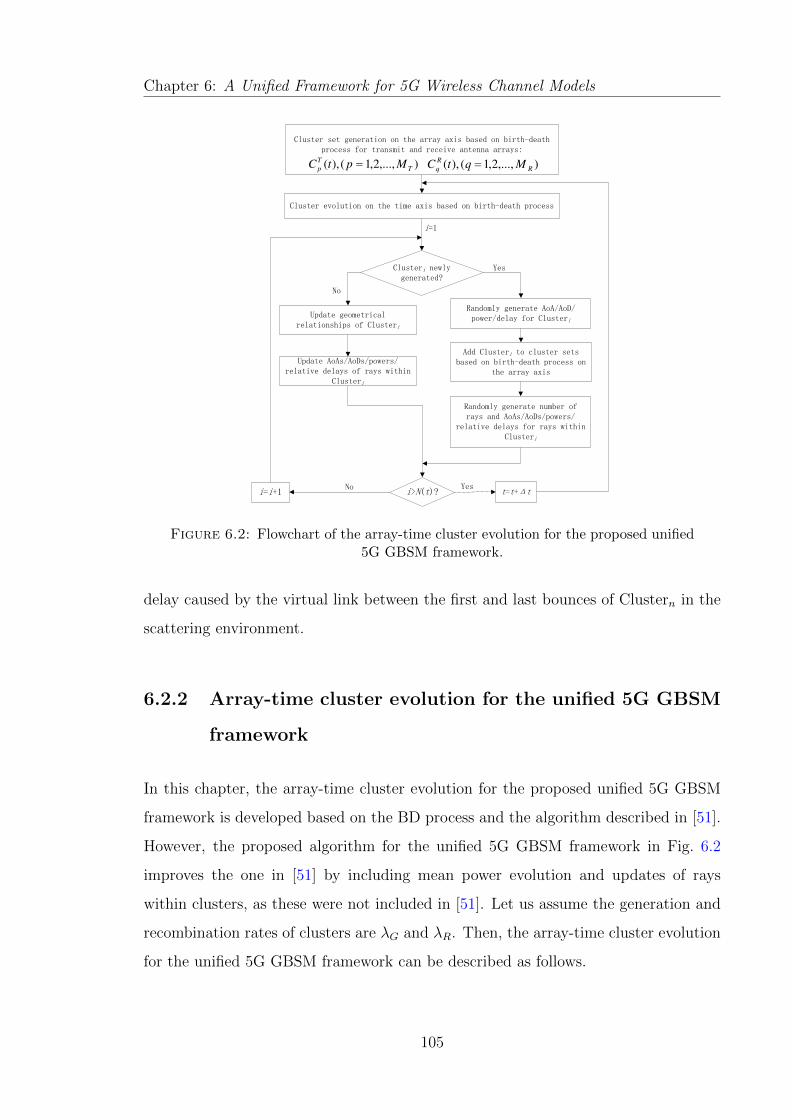
Chapter 6: A Unified Framework for 5G Wireless Channel Models
No
Yes
No Yes
i=1
Cluster set generation on the array axis based on birth-death
process for transmit and receive antenna arrays:
),...,2,1(),( T
T
p MptC ),...,2,1(),( R
R
q MqtC
Cluster evolution on the time axis based on birth-death process
Clusteri newly
generated?
Update geometrical
relationships of Clusteri
Randomly generate AoA/AoD/
power/delay for Clusteri
i>N(t)?i=i+1 t=t+t
Add Clusteri to cluster sets
based on birth-death process on
the array axis
Randomly generate number of
rays and AoAs/AoDs/powers/
relative delays for rays within
Clusteri
Update AoAs/AoDs/powers/
relative delays of rays within
Clusteri
Figure 6.2: Flowchart of the array-time cluster evolution for the proposed unified5G GBSM framework.
delay caused by the virtual link between the first and last bounces of Clustern in the
scattering environment.
6.2.2 Array-time cluster evolution for the unified 5G GBSM
framework
In this chapter, the array-time cluster evolution for the proposed unified 5G GBSM
framework is developed based on the BD process and the algorithm described in [51].
However, the proposed algorithm for the unified 5G GBSM framework in Fig. 6.2
improves the one in [51] by including mean power evolution and updates of rays
within clusters, as these were not included in [51]. Let us assume the generation and
recombination rates of clusters are λG and λR. Then, the array-time cluster evolution
for the unified 5G GBSM framework can be described as follows.
105

Chapter 6: A Unified Framework for 5G Wireless Channel Models
Step 1: An initial set of clusters are generated at time t. The generation procedure
of initial clusters will be described in Section 6.2.3.
Step 2: At time t + ∆t, cluster evolution on the time axis is operated. In principle,
each cluster should have its own survival probability according to the relative motion.
However, for simplicity, mean relative velocities of clusters will be used to calculate
survival probabilities of clusters. Mean relative velocities ∆vR and ∆vT are charac-
terised as ∆vR = E[∥∥vR − vRn
∥∥] and ∆vT = E[∥∥vT − vTn
∥∥]. As a result, the survival
probability PT(∆t) of a cluster after ∆t is computed as
PT(∆t) = e−λR
PF (∆vR+∆vT )∆t
Dsc (6.22)
where PF is the percentage of moving clusters and Dsc is a scenario-dependent co-
efficient describing space correlation [51]. The survivability of each cluster at time
t+ ∆t is determined by PT(∆t). Geometrical relationships, delays, and mean powers
of survived clusters will be updated according to Section 6.2.4. Meanwhile, a random
number of new clusters are generated. This random number is generated according
to the Poisson distribution with mean
E[Nnew(t+ ∆t)] =λGλR
(1− PT(∆t)). (6.23)
Rays and geometrical parameters will be assigned to these new clusters as described
in Section 6.2.3, which also presents the array axis evolution for clusters.
Step 3: When the array-time evolution is finished, the algorithm returns to Step 2 to
enter the next time instant.
6.2.3 Generation of new clusters
For a new cluster, say Clustern, certain parameters such as the number of rays within
the cluster, virtual delay, mean power, angular parameters, and relative delays of
rays need to be assigned to this cluster. These parameters are randomly generated
according to the distributions listed in Table 6.2. The mean power P ′n of clusters is
106

Chapter 6: A Unified Framework for 5G Wireless Channel Models
generated as [30]
P ′n = exp
(−τn
rτ − 1
rτE [τn]
)10−
Zn10 (6.24)
where rτ is the delay scalar (rτ = 2.3 for urban outdoor scenario and rτ = 2.4 for
indoor office scenario [30]) and Zn follows Gaussian distribution N (0, 3) [30]. In
addition, the mean power generation method of a cluster is extended to compute the
mean power of rays within clusters as [143]
P ′n,mn = exp
(−τmn
rτ − 1
rτE [τmn ]
)10−
Zn,mn10 (6.25)
where Zn,mn follows Gaussian distribution N (0, 3) [30]. The mean power of rays is
then scaled by the cluster power as Pn,mn = P ′nP ′n,mn∑
mn
P ′n,mn. The angular parameters φAn ,
φEn ,ϕAn , ϕEn of Clustern are assumed to obey wrapped Gaussian distributions. Then,
the angular parameters of Clustern via the mnth ray can be calculated by adding the
angular offset of the ray, i.e.,
[φAn,mn φ
En,mn ϕ
An,mn ϕ
En,mn
]T=[φAn φ
En ϕ
An ϕ
En
]T+[∆φA ∆φE ∆ϕA ∆ϕE
]T(6.26)
where ∆φA,∆φE,∆ϕA,∆ϕE are angular offsets of the ray, which are assumed to
follow Laplace distributions with zero mean and standard deviation of 0.017 radian
for simplicity.
Table 6.2: Distributions of Parameters of Clusters for the 3-D 5G GBSM.
Parameters Mn τn, τmn , DTn , D
Rn φAn , φEn ,ϕAn , ϕEn
Distributions Poisson Exponential Wrapped Gaussian
Next, which antennas are able to observe the newly generated cluster should be de-
termined. To avoid repeated description, only the receiver side is presented, the
transmitter side follows the same procedure. The survival probability PA of a cluster
evolving from one antenna to an adjacent antenna can be computed as
PA = e−λR
δRDac (6.27)
107

Chapter 6: A Unified Framework for 5G Wireless Channel Models
1: Generate Mn ∼ Pois(λ)
rays for the cluster;
2: Generate virtual delay/mean power/distance for the cluster;3: Generate AoAs/AoDs/relative delays/relative mean powers for the rays within
the cluster;4: Generate discrete q ∼ U (1,MR) and let i = 1, j = 1;5: while (u ∼ U (0, 1) ≤ PA& q + i ≤MR) do6: Add the cluster to CR
(q+i)(t); i = i+ 1;
7: end while8: while (u ∼ U (0, 1) ≤ PA& q − j ≥ 1) do9: Add the cluster to CR
(q−j)(t); j = j + 1;
10: end while
Figure 6.3: Psuedo codes for the new cluster generation algorithm.
where Dac is the scenario-dependent coefficient normalizing antenna spacings [51].
Then, the newly generated cluster is added to the cluster set of a randomly selected
receive antenna. The cluster evolves based on BD process to neighbouring antennas
of the selected receive antenna with survival probability PA. The psuedo codes of new
cluster generation algorithm are shown in Fig. 6.3.
6.2.4 Evolution of survived clusters
In order to highlight time evolution of the proposed model, geometrical relationships,
virtual delays, and mean powers of survived clusters need to be updated from t to
t+ ∆t. To begin with, antenna position vectors are updated as
ARq (t+ ∆t) = AR
q (t) + vR∆t (6.28)
ATp (t+ ∆t) = AT
p (t) + vT∆t. (6.29)
At the same time, distance vectors of clusters need to be adjusted as
DRn (t+ ∆t) = DR
n (t) + vRn∆t (6.30)
108

Chapter 6: A Unified Framework for 5G Wireless Channel Models
DTn (t+ ∆t) = DT
n (t) + vTn∆t. (6.31)
Other distance vectors in (6.4)–(6.10) can be updated accordingly. Delay is updated
as
τn(t+ ∆t) =[∥∥DR
n (t+ ∆t)∥∥+
∥∥DTn (t+ ∆t)
∥∥] /c+ τn(t+ ∆t). (6.32)
The random virtual delay τn(t+∆t) is modeled as τn(t+∆t) = e−∆tς τn(t)+(1−e−
∆tς )X
where X is a random variable independent to τn but identically distributed as τn and
ς is a scenario-dependent parameter describing the coherence of virtual links. Thus,
the updated delay will carry information of the delay in the previous time instant.
Another important aspect is the evolution of cluster mean power. Constant cluster
mean powers were assumed in [42] and [51], which were not sufficient to characterise
time evolution of the channel. Therefore, in this chapter, with the assumption that
the cluster mean powers satisfy the inverse square law, the time evolution of cluster
mean power can be expressed as (Derivations in Appendix B)
Pn,mn(t+ ∆t) = Pn,mn(t)3τn(t)− 2τn(t+ ∆t) + τmn
τn(t) + τmn. (6.33)
The mean power terms Pn,mn in the mean power evolution in (6.33) are not normalised.
They need to be normalised such that Pn,mn = Pn,mn/∑n,mn
Pn,mn before being plugged
into (6.16).
6.2.5 Adaptation to scenarios
The proposed unified 5G GBSM framework can easily be adapted to support various
scenarios by adjusting certain parameters of the channel model.
1. By setting the numbers of antennas (MR and MT ) as relative small numbers,
the wavefronts will automatically be approximated by plane wavefronts. Also,
the cluster evolution on the array axis will become insignificant. In this case,
109

Chapter 6: A Unified Framework for 5G Wireless Channel Models
Figure 6.4: Diagram of combinations of scenarios from the proposed unified 5GGBSM framework.
the unified 5G GBSM framework is reduced to a conventional MIMO channel
model.
2. By setting the velocity of the transmitter vT = 0, the transmitter will be static.
As a result, a Fixed-to-Mobile (F2M) MIMO channel model can be obtained.
In the same way, a Fixed-to-Fixed (F2F) MIMO channel model can be formed
by setting both the transmitter and receiver static, i.e., vT = vR = 0.
3. By setting the relative delays of rays as 0, i.e., τmn = 0, rays within a cluster
will become irresolvable. Consequently, the mmWave MIMO channel model is
simplified as a normal wideband MIMO channel model.
4. By setting all elevation angles as zeros, i.e., υRE(t) = υTE(t) = φEn (t) = ϕEn (t) = 0,
the impacts of elevation angles are ignored. Then, a 2-D MIMO channel model
can be achieved.
Combinations of scenarios can be obtained by properly adjusting these settings. Chan-
nel models for F2F normal wideband 3-D massive MIMO, HST normal wideband 3-D
conventional MIMO, F2F mmWave 3-D conventional MIMO, and M2M normal wide-
band 2-D conventional MIMO are shown in Fig. 6.4 as examples.
110

Chapter 6: A Unified Framework for 5G Wireless Channel Models
6.3 Statistical Property Analysis
6.3.1 Time-variant PDP
The time-variant Power Delay Profile (PDP) Λ(t, τ) of the channel can be expressed
as [34]
Λ(t, τ) =
N(t)∑n
Mn∑mn
Pn,mn(t)δ (τ − τn(t)− τmn) . (6.34)
The time-variant properties of PDP are caused by the time-dependent mean powers
and delays of rays. These are related to the geometrical relationship updates of the
scattering environment.
6.3.2 Stationary interval
The stationary interval is utilised in [2] to measure for the estimated period within
which the channel can be regarded as stationary. The definition of the stationary
interval is the maximum time length within which the autocorrelation function of the
PDP exceeds the 80% threshold [2]. It should be noticed that the 80% threshold
in [2] is empirical and can be adjusted according to requirements. Also, the definition
of stationary interval in [2] would fail to work if the autocorrelation function of the
PDP is not monotonically decreasing or has multiple crossing points at the threshold.
Therefore, it would be more accurate if the stationary interval is defined as the first
point crossing the 80% threshold. An improved definition of the stationary interval
I(t) at time t is proposed as
I(t) = inf
∆t|RΛ(t,∆t)≤0.8
(6.35)
111

Chapter 6: A Unified Framework for 5G Wireless Channel Models
where inf · calculates the infimum of a function and RΛ(t,∆t) is the normalised au-
tocorrelation function of the PDP defined by [2]
RΛ(t,∆t) =
∫Λ(t, τ)Λ(t+ ∆t, τ)dτ
max∫
Λ(t, τ)dτ,∫
Λ(t+ ∆t, τ)dτ . (6.36)
6.3.3 Time-variant transfer function
The time-variant transfer function Hqp(ξ, t) is the Fourier transform of the channel
impulse response with respect to delay, which can be expressed as [34]
Hqp(ξ, t) =
∞∫−∞
hqp(t, τ)e−j2πξτdτ
=
√K
K + 1hLOSqp (t)e−j2πξτ
LOS(t) +
√1
K + 1
N(t)∑n=1
Mn(t)∑mn=1
hqp,n,mn(t)e−j2πξ[τn(t)+τmn ]
(6.37)
where ξ is frequency.
6.3.4 STFCF
To study the correlation properties, the Space-Time-Frequency Correlation Function
(STFCF) ρqp,q′p′(δT , δR,∆ξ,∆t; ξ, t) can be calculated as [34]
ρqp,q′p′(δT , δR,∆ξ,∆t; ξ, t) = E[H∗qp(ξ, t)Hq′p′(ξ + ∆ξ, t+ ∆t)
]. (6.38)
LOS and NLOS components are assumed uncorrelated for simplicity, (6.38) can be
written as the sum of the correlation of the LOS component and the correlation of
the NLOS components, i.e.,
ρqp,q′p′(δT , δR,∆ξ,∆t; ξ, t) = ρLOSqp,q′p′(δT , δR,∆ξ,∆t; ξ, t) + ρNLOS
qp,q′p′(δT , δR,∆ξ,∆t; ξ, t).
(6.39)
112
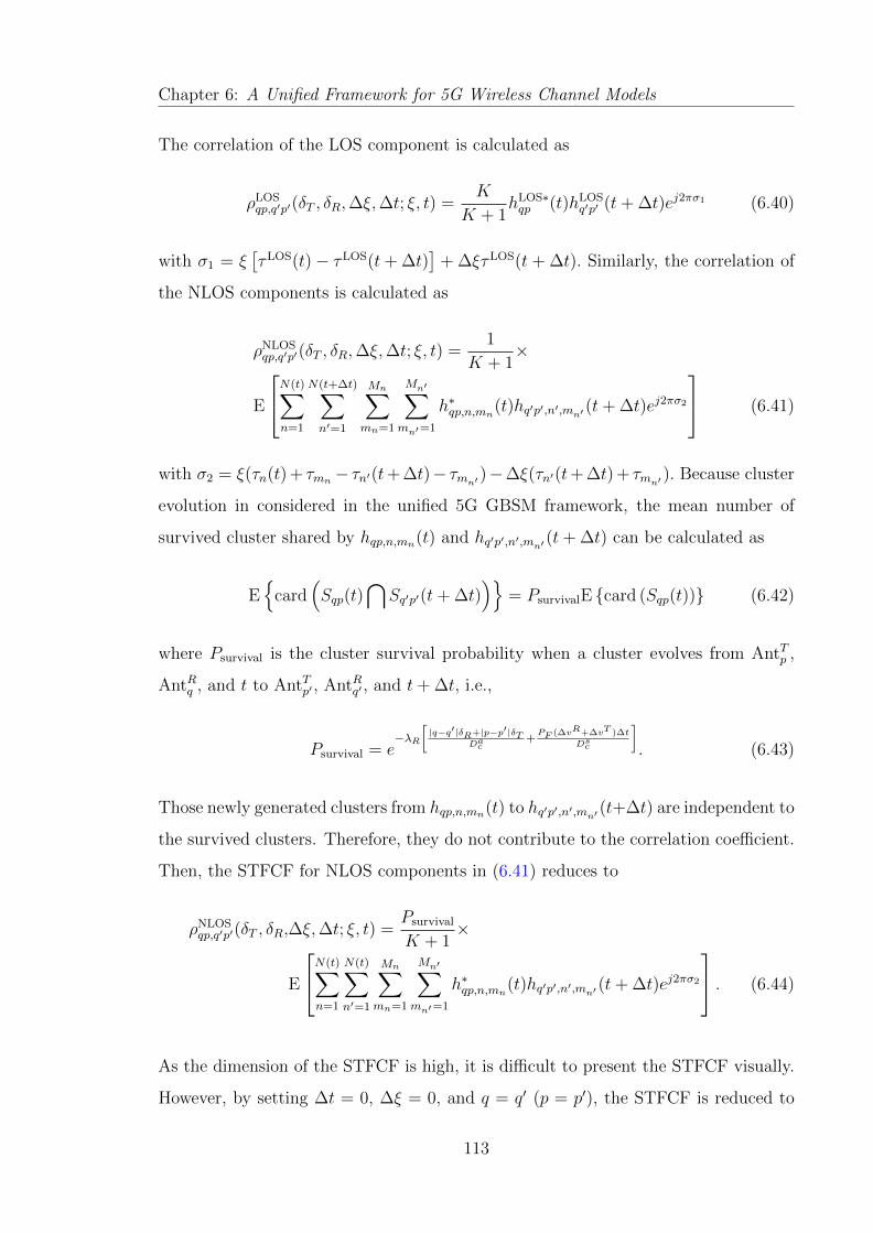
Chapter 6: A Unified Framework for 5G Wireless Channel Models
The correlation of the LOS component is calculated as
ρLOSqp,q′p′(δT , δR,∆ξ,∆t; ξ, t) =
K
K + 1hLOS∗qp (t)hLOS
q′p′ (t+ ∆t)ej2πσ1 (6.40)
with σ1 = ξ[τLOS(t)− τLOS(t+ ∆t)
]+ ∆ξτLOS(t + ∆t). Similarly, the correlation of
the NLOS components is calculated as
ρNLOSqp,q′p′(δT , δR,∆ξ,∆t; ξ, t) =
1
K + 1×
E
N(t)∑n=1
N(t+∆t)∑n′=1
Mn∑mn=1
Mn′∑mn′=1
h∗qp,n,mn(t)hq′p′,n′,mn′ (t+ ∆t)ej2πσ2
(6.41)
with σ2 = ξ(τn(t) + τmn − τn′(t+ ∆t)− τmn′ )−∆ξ(τn′(t+ ∆t) + τmn′ ). Because cluster
evolution in considered in the unified 5G GBSM framework, the mean number of
survived cluster shared by hqp,n,mn(t) and hq′p′,n′,mn′ (t+ ∆t) can be calculated as
E
card(Sqp(t)
⋂Sq′p′(t+ ∆t)
)= PsurvivalE card (Sqp(t)) (6.42)
where Psurvival is the cluster survival probability when a cluster evolves from AntTp ,
AntRq , and t to AntTp′ , AntRq′ , and t+ ∆t, i.e.,
Psurvival = e−λR
[|q−q′|δR+|p−p′|δT
Dac+PF (∆vR+∆vT )∆t
Dsc
]. (6.43)
Those newly generated clusters from hqp,n,mn(t) to hq′p′,n′,mn′ (t+∆t) are independent to
the survived clusters. Therefore, they do not contribute to the correlation coefficient.
Then, the STFCF for NLOS components in (6.41) reduces to
ρNLOSqp,q′p′(δT , δR,∆ξ,∆t; ξ, t) =
Psurvival
K + 1×
E
N(t)∑n=1
N(t)∑n′=1
Mn∑mn=1
Mn′∑mn′=1
h∗qp,n,mn(t)hq′p′,n′,mn′ (t+ ∆t)ej2πσ2
. (6.44)
As the dimension of the STFCF is high, it is difficult to present the STFCF visually.
However, by setting ∆t = 0, ∆ξ = 0, and q = q′ (p = p′), the STFCF is reduced to
113

Chapter 6: A Unified Framework for 5G Wireless Channel Models
the receive (transmit) space Cross-Correlation Function (CCF). Similarly, by setting
q = q′, p = p′, and ∆t = 0, the STFCF is reduced to the time-variant Frequency
Correlation Function (FCF).
6.4 Results and Analysis
In the simulation of the channel, we assumed that the generation rate λG and the
recombination rate λR are set as λG = 80/m [100] and λR = 4/m to fix the mean
number of clusters as 20 [30]. The percentage of moving clusters is PF = 0.3 [100].
The estimated cluster parameters are listed in Table 6.3. Their distributions can be
referred to Table 6.2. Estimation of cluster parameters is based on the minimum
mean squared error (MMSE) criterion. One parameter is estimated via the MMSE
criterion while keeping other parameters fixed. The procedure is performed on every
parameter. All parameters can be modified subject to measurements.
Table 6.3: Simulation parameters for different scenarios.
F2F normal wideband 3-D massive MIMO HST normal wideband 3-D conventional MIMOParameters Mean Standard deviation Parameters Mean Standard deviation
Mn 20 0 Mn 20 0τn 930 ns 930 ns τn 930 ns 930 nsτmn
0 ns 0 ns τmn0 ns 0 ns
DTn 30 m 20 m DT
n 30 m 20 mDR
n 25 m 15 m DRn 25 m 15 m
φAn 0.78 rad 1.15 rad φAn 0.78 rad 0.90 radφEn 0.78 rad 0.18 rad φEn 0.78 rad 0.18 radϕAn 1.05 rad 0.54 rad ϕA
n 1.05 rad 0.54 radϕEn 0.78 rad 0.11 rad ϕE
n 0.78 rad 0.11 radM2M normal wideband 2-D conventional MIMO F2F mmWave 3-D conventional MIMOParameters Mean Standard deviation Parameters Mean Standard deviation
Mn 20 0 Mn 15 3.87τn 930 ns 930 ns τn 305 ns 305 nsτmn
0 ns 0 ns τmn3 ns 3 ns
DTn 30 m 20 m DT
n 5 m 3 mDR
n 25 m 15 m DRn 5 m 3 m
φAn 0.78 rad 0.91 rad φAn 0.78 rad 0.91 radφEn 0 rad 0 rad φEn 0.78 rad 0.18 radϕAn 1.04 rad 0.53 rad ϕA
n 1.04 rad 0.53 radϕEn 0 rad 0 rad ϕE
n 0.78 rad 0.11 rad
114

Chapter 6: A Unified Framework for 5G Wireless Channel Models
0 0.05 0.1 0.15 0.2 0.25 0.3 0.35 0.4 0.45 0.50
0.1
0.2
0.3
0.4
0.5
0.6
0.7
0.8
0.9
1
Time difference, ∆t (s)
Norm
alizedabsolute
timeACF
Simulation model, Cluster1Simulation, Cluster1Simulation model, Cluster2Simulation, Cluster2
Figure 6.5: Comparison between the normalised ACFs of Cluster1 and Cluster2 ofthe normal wideband conventional MIMO channel model (fc = 2GHz, ‖D‖ = 200m,MR = MT = 2, δR = δT = 0.5λ, ∆vR = ∆vT = 0m/s, |vT | = 0,|vR| = 5m/s,
υTE = π6 , υTA = π
3 , υRE = υRA = π4 , Da
c = 50m, M1 = M2 = 81, ς = 7s, NLOS).
To validate the correctness of the proposed unified 5G GBSM framework, the Auto-
correlation Functions (ACFs) of the simulation model and simulation of the normal
wideband conventional MIMO channel model are compared in Fig. 6.5. It should be
noted that these ACFs are normalised with respect to Cluster1. It can be seen from
Fig. 6.5 that the simulated ACFs well align with the ACFs of the simulation model
for both Cluster1 and Cluster2.
The receiver normalised space CCFs of the F2F normal wideband 3-D massive MIMO
channel model are shown in Fig. 6.6. The correlation coefficients drop to a relatively
low level when the antenna index difference is larger than 2. In addition, comparison
between the space CCF of the channel model and measured space CCF in [1, Fig. 10]
is provided. Although the proposed channel model slightly overestimates correlation
at the tail, the space CCF of the channel model aligns well with the measured data
when the antenna index difference is less than 3.
The Complementary Cumulative Distribution Function (CCDF) of the stationary
interval of the HST normal wideband 3-D conventional MIMO channel model is shown
in Fig. 6.7. The median of the stationary interval is approximately 40 ms. Meanwhile,
115
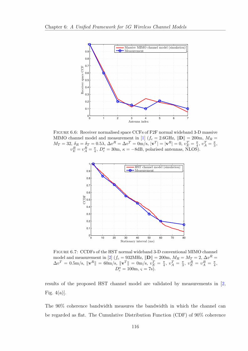
Chapter 6: A Unified Framework for 5G Wireless Channel Models
0 1 2 3 4 5 6 70
0.1
0.2
0.3
0.4
0.5
0.6
0.7
0.8
0.9
1
Antenna index
Receiverspace
CCF
Massive MIMO channel model (simulation)Measurement
Figure 6.6: Receiver normalised space CCFs of F2F normal wideband 3-D massiveMIMO channel model and measurement in [1] (fc = 2.6GHz, ‖D‖ = 200m, MR =MT = 32, δR = δT = 0.5λ, ∆vR = ∆vT = 0m/s, |vT | = |vR| = 0, υTE = π
4 , υTA = π3 ,
υRE = υRA = π4 , Da
c = 30m, κ = −8dB, polarised antennas, NLOS).
0 10 20 30 40 50 60 70 800
0.1
0.2
0.3
0.4
0.5
0.6
0.7
0.8
0.9
1
Stationary interval (ms)
CCDF
HST channel model (simulation)Measurement
Figure 6.7: CCDFs of the HST normal wideband 3-D conventional MIMO channelmodel and measurement in [2] (fc = 932MHz, ‖D‖ = 200m, MR = MT = 2, ∆vR =∆vT = 0.5m/s, ‖vR‖ = 60m/s, ‖vT ‖ = 0m/s, υTE = π
4 , υTA = π3 , υRE = υRA = π
4 ,Dac = 100m, ς = 7s).
results of the proposed HST channel model are validated by measurements in [2,
Fig. 4(a)].
The 90% coherence bandwidth measures the bandwidth in which the channel can
be regarded as flat. The Cumulative Distribution Function (CDF) of 90% coherence
116

Chapter 6: A Unified Framework for 5G Wireless Channel Models
0 0.5 1 1.5 2 2.5 3 3.5 4
x 106
0
0.1
0.2
0.3
0.4
0.5
0.6
0.7
0.8
0.9
1
90% Coherence Bandwidth (Hz)
CDF
M2M channel model
Measurement
Suburban
Scenario
Figure 6.8: CDF of 90% coherence bandwidth of the M2M normal wideband 2-Dconventional MIMO channel model and measurement (suburband scenario) in [3](fc = 5.9GHz, ‖D‖ = 400m, ∆vR = ∆vT = 0.5m/s, ‖vT ‖ = ‖vR‖ = 25m/s,
υRA = υRE = π4 , υTA = π
3 , υRE = π4 , Ds
c = 10m, ς = 5s).
bandwidth of the M2M normal wideband 2-D conventional MIMO channel model is
illustrated in Fig. 6.8, which is also validated by that of the measured suburban M2M
channel in [3, Fig. 5(a)].
A snapshot of normalized Angular Power Spectrum (APS) at the receiver of a mmWave
massive MIMO channel is illustrated in Fig. 6.9. The APS is estimated with the MUl-
tiple SIgnal Classification (MUSIC) algorithm [119], [120] using a sliding window of 3
consecutive antennas. It can be observed that the number of clusters is small because
of the high carrier frequency of mmWave. Meanwhile, appearance and disappearance
of clusters on the array axis can also be seen due to the massive MIMO antenna array.
Fig. 6.10 presents the CCDFs of the Root Mean Squared (RMS) delay spread of the
mmWave channel model. The RMS spread of the mmWave channel model is in the
order of 10ns. Scenario 1 and Scenario 2 are the Room H scenario and Room F scenario
in [4, Fig. 5], respectively. Measurement results for different scenarios in [4, Fig. 5]
can be fitted properly by the proposed mmWave channel model.
117

Chapter 6: A Unified Framework for 5G Wireless Channel Models
Window position
Ao
A (
de
gre
es)
5 10 15 20 25 30
0
20
40
60
80
100
120
140
160
180
1
0
Figure 6.9: A snapshot of simulated normalized APS at the receiver of themmWave 2-D massive MIMO channel model (fc = 58GHz, MT = 2, MR = 32,‖D‖ = 6m, δR = δT = 0.5λ, ∆vR = ∆vT = 0m/s, |vT | = |vR| = 0, υTE = π
4 ,υTA = π
3 , υRE = υRA = 0, Dac = 30m, Ds
c = 100m, NLOS).
2 3 4 5 6 7
x 10−8
0
0.1
0.2
0.3
0.4
0.5
0.6
0.7
0.8
0.9
1
RMS delay spread (s)
CCDF
mmWave channel modelMeasurement
Scenario 2Scenario 1
Figure 6.10: CCDFs of RMS delay spread of the F2F mmWave 3-D conventionalMIMO channel model and measurement in [4] (fc = 58GHz, ‖D‖ = 6m, ∆vR =∆vT = 0m/s, ‖vT ‖ = ‖vR‖ = 0m/s, υRA = υRE = π
4 , υTA = π3 , υTE = π
4 , Dsc = 100m,
ς = 7s).
118

Chapter 6: A Unified Framework for 5G Wireless Channel Models
8 10 12 14 16 18 200
1
2
3
4
5
6
7
SNR (dB)
No
rma
lize
d c
ha
nn
el ca
pa
city (
bp
s/H
z)
i.i.d. channel model
3−D unified GBSM framework, polarized antennas
3−D unified GBSM framework, normal antennas
Figure 6.11: Comparison of normalized channel capacities of the unified GBSMframework for massive MIMO channel models with normal and polarized antennas(MR = 8, MT = 32, fc = 2GHz, ‖D‖ = 100m, υRA = π
4 , υTA = π3 , Ds
c = 100m,ς = 7s, υRE = π
4 , υTE = π4 , κ = −8dB).
Channel capacities of the unified GBSM framework with normal and polarized anten-
nas are shown in Fig. 6.11. The channel capacity with polarized antennas is lower than
that with normal antennas. However, the dimensions of antenna arrays are halved
because of the use of polarized antennas.
Fig. 6.12 depicts the channel capacities of the i.i.d. massive MIMO channel model, the
2-D ellipse massive MIMO channel model, the 3-D twin-cluster massive MIMO channel
model, the reduced 2-D twin-cluster massive MIMO channel model, the KBSM–BD–
AA with isotropic scattering environment, the 3-D unified GBSM framework, and the
reduced 2-D unified GBSM framework. The channel capacities of these channel models
are computed using the capacity of frequency selective MIMO channels in [13]. The
channel capacities of those three GBSMs slightly vary with elevation angles considered.
The i.i.d. channel capacity serves as the upper bound of channel capacities while the
capacity of the KBSM–BD–AA with isotropic scattering environment lies between the
i.i.d. channel capacity and the capacities of GBSMs.
119

Chapter 6: A Unified Framework for 5G Wireless Channel Models
8 10 12 14 16 18 200
1
2
3
4
5
6
7
8
SNR (dB)
No
rma
lize
d c
ha
nn
el ca
pa
city (
bp
s/H
z)
i.i.d. channel model
2−D ellipse model
3−D twin−cluster model
3−D unified GBSM framework
2−D twin−cluster model
2−D unified GBSM framework
KBSM−BD−AA
Figure 6.12: Comparison of normalized channel capacities of massive MIMO chan-nel models (MR = 8, MT = 32, fc = 2GHz, ‖D‖ = 100m, υRA = π
4 , υTA = π3 ,
Dsc = 100m, ς = 7s, υRE = π
4 (3-D models only), υTE = π4 (3-D models only)).
6.5 Summary
In this chapter, a unified framework for 5G channel models has been proposed. The
WINNER II and SV channel model have been combined in the unified framework.
The proposed unified 5G GBSM framework can be adapted to various scenarios by
properly setting certain parameters. Simulated statistical properties of the proposed
unified 5G GBSM framework have been compared with measurements. In addition,
3-D features and polarised directional antennas are included. Another important issue
is the modelling of time evolution of the channel, which includes cluster evolution on
the time axis, geometrical relationship updates, and evolution of delays and powers of
rays. For future work, applications of the proposed channel model to 5G system simu-
lators need to be considered. Also, cooperative MIMO channel model with multi-link
correlation and parameters for HST channel model in tunnel scenarios are potential
directions.
120

Chapter 7Conclusions and Future Work
This thesis has presented a wealth of comprehensive research on wireless channel
modelling and simulation for massive MIMO communication systems (i.e., GBSMs
in Chapter 3 and Chapter 4, KBSM in Chapter 5, and a unified framework for 5G
channels in Chapter 6). The importance of our research has been proved and intro-
duced in detail. In this concluding chapter, the key findings of my PhD research are
summarised and several potential future research directions are proposed as well.
7.1 Summary of Results
7.1.1 GBSMs for massive MIMO channels
In Chapter 3, a novel non-stationary wideband multi-confocal ellipse 2-D GBSM for
massive MIMO channels has been proposed. Spherical wavefront has been assumed in
the proposed model to characterise the nearfield effect caused by the increase in the
number of antennas. It has been demonstrated that WSS properties are not available
under the spherical wavefront assumption. In addition, the BD process has been used
in the proposed model to capture the array-time evolution of clusters. Statistical
properties of the channel model such as the STFCF, space CCF, APS, average life
periods of clusters on the array axis, time ACF, FCF, and power imbalance on the
121

Chapter 7: Conclusions and Future Work
antenna array have been studied. The impact of the spherical wavefront assumption
on the statistical properties of the channel model has been investigated. Furthermore,
numerical analysis has shown that the proposed channel model is able to capture
specific characteristics of massive MIMO channel as observed in measurements.
In Chapter 4, we have proposed a novel non-stationary 3-D wideband twin-cluster
channel model along with the corresponding simulation model for massive MIMO
systems with carrier frequencies in the order of GHz. Nearfield effects instead of
farfield effects have been considered in the proposed model. These include the spher-
ical wavefront assumption and a BD process to model non-stationary properties of
clusters such as cluster appearance and disappearance on both the array and time
axes, AoA shifts, received power variations, and Doppler frequency variations on the
antenna array. The impact of elevation angles of clusters on space CCF, time ACF
of the massive MIMO channel model has been studied. Additionally, the Doppler
PSD, standard deviation of Doppler frequencies on the large array, APS, and condi-
tion number of the channel have been investigated. Moreover, it has been shown that
the channel characteristics of the simulation model are consistent with those of the
theoretical model.
7.1.2 KBSM for massive MIMO channels
In Chapter 5, we have proposed a novel KBSM–BD–AA for massive MIMO channels.
The evolution of scatterer sets on the array axis has been abstracted by a survival prob-
ability matrix based on the BD process. With this consideration, the overall antenna
correlation matrix is equivalent to the Hadamard product of the spatial correlation
matrix and the survival probability matrix. Upper and lower bounds of channel ca-
pacities have been analysed in both the high and low SNR regimes when the numbers
of transmit and receive antennas are increasing unboundedly with a constant ratio.
The evolution of scatterer sets on the array axis has been shown to decrease spatial
correlations of KBSM channels.
122

Chapter 7: Conclusions and Future Work
7.1.3 A unified framework for 5G channel models
In Chapter 6, a unified framework for 5G channel models has been proposed. The
proposed unified 5G GBSM framework can be adapted to various scenarios by properly
setting certain parameters, such as massive MIMO systems, HST communications,
M2M communications, and mmWave communications. The proposed 5G channel
model framework is a 3-D non-stationary channel model based on the WINNER II
and SV channel models considering array-time cluster evolution. In addition, 3-D
features and polarised directional antennas have been included. Another important
issue is the modelling of time evolution of the channel, which includes cluster evolution
on the time axis, geometrical relationship updates, and evolution of delays and powers
of rays. Statistical properties of the proposed 5G channel model such as time ACF,
space CCF, APS, CCDF of stationary intervals, CDF of 90% coherence bandwidth,
and CCDF of RMS delay have been investigated to demonstrate its capability of
capturing channel characteristics of various scenarios, with excellent fitting to certain
corresponding measurements.
7.2 Future Research Directions
There are several potential directions of this thesis that can be further expanded.
7.2.1 COST 2100 model for massive MIMO channels
The COST 2100 channel model, a cluster-based GBSM, introduced Visibility Regions
(VRs) to model the spatially-variant nature of massive MIMO channels, i.e., cluster
appearance and disappearance on the array axis [53]. A VR is a region in space
corresponding to a cluster. A cluster is observable to an antenna element if this
antenna element lies within the VR of the cluster. Different antenna elements on a
large array may lie within various VRs. Then, each antenna element may observe its
own set of clusters.
123

Chapter 7: Conclusions and Future Work
The modelling of spatial variance via VRs in the COST 2100 channel model is fun-
damentally different from the method based on BD processes introduced in the twin-
cluster and ellipse channel models in [42], [51], [113]. The COST 2100 channel model
is able to jointly model time and array evolutions with VRs. Also, it was reported
in [53] that parameters of VRs could be estimated based on measured data. For mod-
elling massive MIMO effects at the transmitter and receiver, visibility regions can be
applied to both the BS and UE.
However, the current assumption of a VR is a circular region on the azimuth plane in
[31]–[33], [53]. This may fail to model the 3-D scattering environment, especially when
the transmitter or receiver moves vertically or vertical beamforming for skyscraper
scenario is considered. A potential solution for this is to generalise circular region of a
VR to a sphere in a 3-D space. Meanwhile, the complexity of the COST 2100 channel
modelling for massive MIMO is still under investigation.
7.2.2 Map-based massive MIMO channels
Besides the GBSM discussed in Chapter 3, Chapter 4, and Chapter 6, the METIS
project proposed a novel modelling method for massive MIMO channels named as
the Map-Based Channel Model (MBCM) [47]. The METIS MBCM was established
based on ray tracing techniques. It aimed at tracking each ray from the transmitter
to the receiver. Interactions between rays and shadowing/scattering objects such
as diffraction, specular reflection, diffuse scattering, and blocking were considered.
These shadowing/scattering objects can be randomly generated in the environment
or obtained from a specific scenario.
Since each ray is tracked by the MBCM, massive MIMO channel characteristics such
as spherical wavefront and non-stationary properties of clusters are included in the
model. Additionally, having considered Doppler frequencies at both the transmit-
ter and receiver sides, the METIS MBCM is able to support scenarios where M2M
communications with massive MIMO. However, the ray tracing nature of the MBCM
results in high complexity [47]. The practicality of MBCM is to be justified.
124

Chapter 7: Conclusions and Future Work
7.2.3 Correlation-based massive MIMO channel model
The adaptation of BD to KBSMs can be achieved without extra complexity, because
antenna spatial correlation matrices for KBSMs can be separated easily. However, The
adaptation of BD to Weichselberger or VCR requires further investigations, which will
be an interesting research direction in the future. Further, general CBSM [124] with
extension of BD process on the array axis for massive MIMO channel modelling may
be developed.
7.2.4 Standardised 5G channel model
As standardised 5G channel models are still missing in the literature, attentions should
be paid to the development of standardised models. To achieve this goal, a model cap-
turing key characteristics of massive MIMO and mmWave channels with reasonable
complexity needs to be considered. The unified framework for 5G wireless channels
in Chapter 6 can be used as a starting point. Additionally, large-scale fading, i.e.,
pathloss and shadow fading for massive MIMO should be included in the standard-
ised massive MIMO channel model. Moreover, other scenarios such as cooperative
communications and HST communications in tunnels should be considered as well.
125

Appendix AAntenna Pattern Calculation
In a 3-D space, the geometry of antenna pattern depends on the orientation of anten-
nas. A LCS is constructed along the horizontal polarization, vertical polarization, and
antenna broadside as Fig. A.1 shows. The LCS is obtained by a sequence of rotations
from the GCS [145]. First, a rotation of αT about xG axis is operated. Second, a
rotation of βT about the new yG axis is operated. Third, a rotation of γT about the
new zG axis is operated. These three operations can be expressed as [145]
Gz
Gy
Gx
TD
TE
TJ
TxL
TzL
TyL
(Horizontal polarization)
(Vertical polarization)
(Antenna broadside)
Figure A.1: Diagram of LCS and GCS in the 3-D space.
126

Appendix A: Antenna Pattern Calculation
R =
cos γT − sin γT 0
sin γT cos γT 0
0 0 1
cos βT 0 sin βT
0 1 0
− sin βT 0 cos βT
1 0 0
0 cosαT − sinαT
0 sinαT cosαT
. (A.1)
Let a and b be positions vectors in the GCS, and let (x, y, z)T be the coordinates of
a−b in the LCS. Then, (x, y, z)T = R(a−b). Let w(x, y) be the four-quadrant inverse
tangent function [146] of x and y, and let θ = w(y, x) and φ = w(z,√x2 + y2). Then,
the antenna patterns can be computed as FH(a,b) = G(θ, φ) cos θ and FV (a,b) =
G(θ, φ) sin θ. In Chapter 6, dipole antennas are assumed at the transmitter side. In
this case [147],
G(θ, φ) =√
1.64cos(π2
cos φ)
sin φ. (A.2)
At the receiver side, calculation follows a similar procedure. Omnidirectional antennas
are assumed at the receiver side. In this case, G(θ, φ) = 1. The rotation angles αT ,
αR, βT , βR, γT , and γR are all set as π15
for simplicity, which can be modified according
to realistic settings.
127

Appendix BTime Evolution of Ray Mean Powers
Let us consider the time interval between t and t+ ∆t, where ∆t is small. Then, the
cluster mean power difference ∆Pn,mn(t) between these two time instants is computed
as
∆Pn,mn(t) = Pn,mn(t+ ∆t)− Pn,mn(t). (B.1)
With the assumption of the inverse power law, the cluster mean power is inversely
proportional to the ηth (η > 1) power of travel distance, i.e.,
Pn,mn(t) =C
[τn(t) + τn,mn ]η cη(B.2)
where C is a constant. The derivative of Pn,mn(t) with respect to t is obtained by
∆Pn,mn(t)
∆t=
(C
[τn(t) + τn,mn ]η cη
)′= −η C
[τn(t) + τn,mn ]η+1 cη(τn(t))′
= −η C[τn(t) + τn,mn ]η+1 cη
[τn(t+ ∆t)− τn(t)]
∆t. (B.3)
Thus, the cluster mean power evolution in terms of time can be derived as
∆Pn,mn(t)
Pn,mn(t)=
−ητn(t) + τn,mn
[τn(t+ ∆t)− τn(t)]
∆t∆t. (B.4)
128

Appendix B: Time Evolution of Ray Mean Powers
Re-ordering the above equation, the update formula is
Pn,mn(t+ ∆t) = Pn,mn(t)(η + 1)τn(t)− ητn(t+ ∆t) + τn,mn
τn(t) + τn,mn. (B.5)
With the assumption of the inverse square law (η = 2), (6.33) is obtained.
129

References
[1] S. Payami and F. Tufvesson, “Channel measurements and analysis for very large
array systems at 2.6GHz,” in Proc. of the 6th European Conference on Antennas
and Propagation, Prague, Czech Republic, Mar. 2012.
[2] C. Chen, Z. Zhong, and B. Ai, “Stationarity intervals of time-variant channel in
high speed railway scenario,” J. China Commun., vol. 9, no. 8, pp. 64–70, Aug.
2012.
[3] L. Cheng, B. Henty, R. Cooper, D. D. Stancil, and F. Bai, “Multi-path propa-
gation measurements for vehicular networks at 5.9 GHz,” in Proc. WCNC’08.,
Las Vegas, US, Apr. 2008, pp. 1239–1244.
[4] P. F. M. Smulders and A. G. Wagemans, “Frequency-domain measurement of
the millimeter wave indoor radio channel,” IEEE Trans. Instrum. Meas., vol. 44,
no. 6, pp. 1017–1022, Dec. 1995.
[5] Nokia Networks. Looking ahead to 5G. White Paper. Available:
http://networks.nokia.com/sites/default/files/document/5g white paper 0.pdf.
[6] 5GNOW. 5G cellular communications scenarios and system requirements.
White Paper. Available:
http://www.5gnow.eu/wp-content/uploads/2015/04/5GNOW D2.1 v1.0 0.pdf.
130

References
[7] METIS. Scenarios, requirements and KPIs for 5G mobile and wireless system.
Available:
https://www.metis2020.com/wp-content/uploads/deliverables/METIS D1.1 v1.pdf.
[8] IMT-2020 Promotion Group. 5G visions and requirements. White Paper.
Available:
http://euchina-ict.eu/wp-content/uploads/2015/03/IMT-20205GPG-WHITE-
PAPER-ON-5G-VISION-AND-REQUIREMENTS V1.0.pdf.
[9] E. Dahlman, G. Mildh, S. Parkvall, J. Peisa, J. Sachs, and Y. Selen, “5G radio
access,” Ericsson Review, vol. 6, pp. 1–7, 2014.
[10] Samsung. 5G vision. White Paper. Available:
http://www.samsung.com/global/business-images/insights/2015/Samsung-5G-
Vision-0.pdf.
[11] Qualcomm. 1000x data challenge. White Paper. Available:
https://www.qualcomm.com/invention/technologies/1000x.
[12] Huawei. 5G a technology vision. White Paper. Available:
http://www.huawei.com/5gwhitepaper/.
[13] A. Paulraj, R. Nabar, and D. Gore, Introduction to Space-Time Wireless Com-
munications., Cambridge University Press, Cambridge, 2008.
[14] IEEE 802.16 WG, 802.16m Evaluation methodology document, 802.16m-
08/004r5, Jan. 1999.
[15] S. Sesia, I. Toufik, and M. Baker, LTE–The UMTS Long Term Evolution: From
Theory to Practice., 2nd ed., John Wiley & Sons, West Sussex, 2011.
[16] G. J. Foschini and M. J. Gans, “On limits of wireless communications in a fading
environment when using multiple antennas,” Wireless Pers. Commun., vol. 6,
no. 3, pp. 311–335, Mar. 1998.
[17] D. Gesbert, M. Shafi, D. Shiu, P. J. Smith, and A. Naguib, “From theory to
practice: an overview of MIMO space-time coded wireless systems,” IEEE J.
Sel. Areas Commun., vol. 21, no. 3, pp. 281–302, Apr. 2003.
131
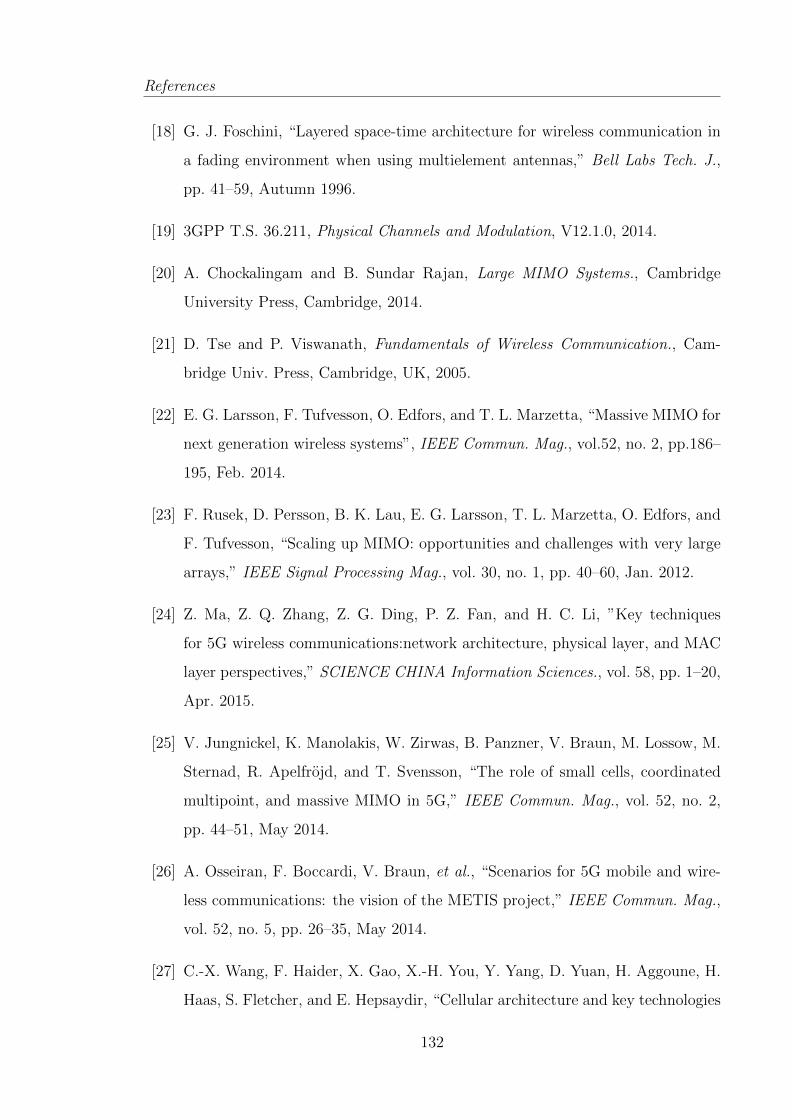
References
[18] G. J. Foschini, “Layered space-time architecture for wireless communication in
a fading environment when using multielement antennas,” Bell Labs Tech. J.,
pp. 41–59, Autumn 1996.
[19] 3GPP T.S. 36.211, Physical Channels and Modulation, V12.1.0, 2014.
[20] A. Chockalingam and B. Sundar Rajan, Large MIMO Systems., Cambridge
University Press, Cambridge, 2014.
[21] D. Tse and P. Viswanath, Fundamentals of Wireless Communication., Cam-
bridge Univ. Press, Cambridge, UK, 2005.
[22] E. G. Larsson, F. Tufvesson, O. Edfors, and T. L. Marzetta, “Massive MIMO for
next generation wireless systems”, IEEE Commun. Mag., vol.52, no. 2, pp.186–
195, Feb. 2014.
[23] F. Rusek, D. Persson, B. K. Lau, E. G. Larsson, T. L. Marzetta, O. Edfors, and
F. Tufvesson, “Scaling up MIMO: opportunities and challenges with very large
arrays,” IEEE Signal Processing Mag., vol. 30, no. 1, pp. 40–60, Jan. 2012.
[24] Z. Ma, Z. Q. Zhang, Z. G. Ding, P. Z. Fan, and H. C. Li, ”Key techniques
for 5G wireless communications:network architecture, physical layer, and MAC
layer perspectives,” SCIENCE CHINA Information Sciences., vol. 58, pp. 1–20,
Apr. 2015.
[25] V. Jungnickel, K. Manolakis, W. Zirwas, B. Panzner, V. Braun, M. Lossow, M.
Sternad, R. Apelfrojd, and T. Svensson, “The role of small cells, coordinated
multipoint, and massive MIMO in 5G,” IEEE Commun. Mag., vol. 52, no. 2,
pp. 44–51, May 2014.
[26] A. Osseiran, F. Boccardi, V. Braun, et al., “Scenarios for 5G mobile and wire-
less communications: the vision of the METIS project,” IEEE Commun. Mag.,
vol. 52, no. 5, pp. 26–35, May 2014.
[27] C.-X. Wang, F. Haider, X. Gao, X.-H. You, Y. Yang, D. Yuan, H. Aggoune, H.
Haas, S. Fletcher, and E. Hepsaydir, “Cellular architecture and key technologies
132

References
for 5G wireless communication networks,” IEEE Commun. Mag., vol. 52, no. 2,
pp. 122–130, Feb. 2014.
[28] B. N. Getu and J. B. Andersen, “The MIMO cube – a compact MIMO antenna,”
IEEE Trans. Wireless Commun., vol. 4, no. 3, pp. 1136–1141, May 2005.
[29] A. L. Moustakas, H. U. Baranger, L. Balents, A. M. Sengupta, and S. H. Simon,
“Communication through a diffusive medium: coherence and capacity,” Science,
vol. 287, no. 5451, pp. 287–290, Jan. 2000.
[30] P. Kyosti, et al., “WINNER II channel model”, ver 1.1, Sept. 2007. Available:
http://www.ist-winner.org/WINNER2-Deliverables/D1.1.2v1.1.pdf.
[31] L. Liu, C. Oestges, J. Poutanen, K. Haneda, P. Vainikainen, F. Quitin, F.
Tufvesson, and P. D. Doncker, “The COST 2100 MIMO channel model,” IEEE
Commun. Mag., vol. 19, no. 6, pp. 92–99, Dec. 2012.
[32] M. F. Zhu, G. Eriksson, and F. Tufvesson, “The COST 2100 channel model:
parameterization and validation based on outdoor MIMO measurements at 300
MHz,”,IEEE Trans. Wireless Commun., vol. 12, no. 2, pp. 888–897, Feb, 2013.
[33] R. Verdone and A. Zanella, Pervasive Mobile and Ambient Wireless Communi-
cations: COST Action 2100., Springer, London, 2012.
[34] M. Patzold, Mobile Radio Channels., 2nd ed., John Wiley & Sons, West Sussex,
2012.
[35] A. J. Grant, “Performance analysis of transmit beamforming,” IEEE Trans.
Commun., vol. 53, no. 4, pp. 738–744, Apr. 2005.
[36] A. M. Tulino and S. Verdu, Random Matrix Theory and Wireless Communica-
tions., Foundations and Trends r in Communications and Information Theory,
vol. 1, no. 1, pp. 1-182, June 2004. doi: 10.1561/0100000001.
[37] A. Lozano, A. M. Tulino, and S. Verdu, “Multiple-antenna capacity in the low-
power regime,” IEEE Trans. Inf. Theory, vol. 49, no. 10, pp. 2527–2544, Oct.
2003.
133

References
[38] A. G. Zajic and G. L. Stuber, “Space-time correlated mobile-to-mobile channels:
modelling and simulation,” IEEE Trans. Veh. Technol., vol. 57, no. 2, pp. 715–
726, Mar. 2008.
[39] M. Patzold, B. O. Hogstad, and N. Youssef, “Modeling, analysis, and simulation
of MIMO mobile-to-mobile fading channels,” IEEE Trans. Wireless. Commun.,
vol. 7, no. 2, pp. 510–520, Feb. 2008.
[40] A. Ghazal, C.-X. Wang, B. Ai, D. Yuan, and H. Haas, “A non-stationary
wideband MIMO channel model for high-mobility intelligent transportation sys-
tems,” IEEE Trans. Intell. Transp. Syst., vol. 16, no. 2, pp. 885–897, Apr. 2015.
[41] B. O. Hogstad, M. Patzold, and A. Chopra, “A study on the capacity of narrow-
and wideband MIMO channel models,” in Proc. IST’06, Myconos, Greece, June
2006, pp. 1–6.
[42] S. Wu, C. -X. Wang, H. Haas, el-H. M. Aggoune, M. M. Alwakeel, and B. Ai,
“A non-stationary wideband channel model for Massive MIMO communication
systems,” IEEE Trans. Wireless Commun., vol. 14, no. 3, pp. 1434–1446, Mar.
2015.
[43] X. Cheng, C. -X. Wang, D. I. Laurenson, S. Salous, and A. V. Vasilakos, “An
adaptive geometry-based stochastic model for non-isotropic MIMO mobile-to-
mobile channels,” IEEE Trans. Wireless Commun., vol. 8, no. 9, pp. 4824–4835,
Sep. 2009.
[44] X. Cheng, C.-X. Wang, B. Ai, and H. Aggoune, “Envelope level crossing rate
and average fade duration of non-isotropic vehicle-to-vehicle Ricean fading chan-
nels,” IEEE Trans. Intell. Transp. Syst., vol. 15, no. 1, pp. 62–72, Feb. 2014.
[45] X. Cheng, C.-X. Wang, H. Wang, X. Gao, X.-H. You, D. Yuan, B. Ai, Q. Huo,
L. Song, and B. Jiao, “Cooperative MIMO channel modeling and multi-link
spatial correlation properties,” IEEE J. Sel. Areas Commun., vol. 30, no. 2,
pp. 388–396, Feb. 2012.
134
References
[46] 3GPP T.S. 25.996, Spatial channel model for multiple input multiple output
(MIMO) simulations, V11.0.0, 2012.
[47] L. Raschkowski, et al., “METIS Channel Models”. Available:
https://www.metis2020.com/wp-content/uploads/deliverables/METIS D1.4 v1.0.pdf.
[48] Report ITU-R M.2135-1, “Guidelines for evaluation of radio interface technolo-
gies for IMT-Advanced”, 2009.
[49] A. Kuchar, J. -P. Rossi, and E. Bonek, “Directional macro-cell channel charac-
terization from urban measurements,” IEEE Trans. Antennas Propag., vol. 48,
no. 2, pp. 137–146, Feb. 2000.
[50] H. Hofstetter, A. F. Molisch, and N. Czink, “A twin-cluster MIMO channel
model,” in Proc. IEEE EuCAP’06, Nice, France, Nov. 2006, pp. 1–8.
[51] S. Wu, C. -X. Wang, el-H. M. Aggoune, M. M. Alwakeel, and Y. He, “A non-
stationary 3-D wideband twin-cluster model for 5G massive MIMO channels,”
IEEE J. Sel. Areas Commun., vol. 32, no. 6, pp. 1207–1218, June 2014.
[52] N. Czink and C. Oestges, “The COST 273 MIMO channel model: three kinds
of clusters,” in Proc. ISSSTA’08, Bologna, Italy, Aug. 2008, pp. 282–286.
[53] X. Gao, F. Tufvesson, and O. Edfors, “Massive MIMO channels-measurements
and models,” in Proc. ASILOMAR’13, Pacific Grove, USA, Nov. 2013, pp. 280–
284.
[54] A. G. Zajic and G. L. Stuber, “Three-dimensional modeling, simulation, and
capacity analysis of space-time correlated mobile-to-mobile channels,” IEEE
Trans. Veh. Technol., vol. 57, no. 4, pp. 2042–2054, July 2008.
[55] A. G. Zajic and G. L. Stuber, “Three-dimensional modeling and simulation of
wideband MIMO mobile-to-mobile channels,” IEEE Trans. Wireless Commun.,
vol. 8, no. 3, pp. 1260–1275, Mar. 2009.
[56] Y. Yuan, C.-X. Wang, X. Cheng, B. Ai, and D. I. Laurenson, “Novel 3D
geometry-based stochastic models for non-isotropic MIMO vehicle-to-vehicle
135

References
channels,” IEEE Trans. Wireless Commun., vol. 13, no. 1, pp. 298–309, Jan.
2014.
[57] Y. Yuan, C. -X. Wang, Y. He, el-H. M. Aggoune, and M. M. Alwakeel, “Novel
3D wideband non-stationary geometry-based stochastic models for non-isotropic
MIMO vehicle-to-vehicle channels,” IEEE Trans. Wireless Commun., accepted
for publication.
[58] K. Kalliola, H. Laitinen, P. Vainikainen, M. Toeltsch, J. Laurila, and E. Bonek,
“3-D double-directional radio channel characterization for urban macrocellular
applications,” IEEE Trans. Antennas Propag., vol. 51, no. 11, pp. 3122–3133,
Nov. 2003.
[59] A. Kammoun, H. Khanfir, Z. Altman, M. Debbah, and M. Kamoun, “Prelim-
inary results on 3D channel modeling: from theory to standardization,” IEEE
J. Sel. Areas Commun., vol. 32, no. 6, pp. 1219–1229, June 2014.
[60] T. A. Thomas, F. W. Vook, E. Visotsky, E. Mellios, G. S. Hilton, and A. R.
Nix, “3D Extension of the 3GPP/ITU channel model.” in Proc. IEEE VTC’13-
Spring, Dresden, Germany, June 2013, pp. 1–5.
[61] D. S. Baum, J. Hansen, and J. Salo, “An interim channel model for beyond-3G
systems: extending the 3GPP spatial channel model (SCM),” in Proc. IEEE
VTC’05 Spring, vol. 5, Stockholm, Sweden, May 2005, pp. 3132–3136.
[62] P. Heino, et al., “WINNER+ final channel models”, ver 1.0, June 2010.
Available:
http://projects.celtic-initiative.org/winner+/WINNER+%20Deliverables/D5.3 v1.0.pdf.
[63] 3GPP T.R. 36.814, Further advancements for E-UTRA physical layer aspects,
V9.0.0, 2010.
[64] M. Wu, B. Yin, G. Wang, C. Dick, J. R. Cavallaro, and C. Studer, “Large-
scale MIMO detection for 3GPP LTE: algorithms and FPGA implementations,”
IEEE J. Sel. Topics Signal Process., vol. 8, no. 5, pp. 916–929, Oct. 2014.
136
References
[65] A. A. M. Saleh and R. A. Valenzuela, “A statistical model for indoor multipath
propagation,” IEEE J. Sel. Areas Commun., vol. 5, no. 2, pp. 128–137, Feb.
1987.
[66] A. Maltsev et al., “Channel models for 60 GHz WLAN systems”. Available:
https://mentor.ieee.org/802.11/dcn/09/11-09-0334-06-00ad-channel-models-
for-60-ghz-wlan-systems.doc.
[67] L. Zheng and D. N. C. Tse, “Diversity and multiplexing: a fundamental trade-
off in multiple-antenna channels,” IEEE Trans. Inf. Theory., vol. 49, no. 5,
pp. 1073–1096, May 2003.
[68] S. K. Mohammed and E. G. Larsson, “Per-antenna constant envelope precoding
for large multi-user MIMO systems,” IEEE Trans. Commun., vol. 61, no. 3,
pp. 1059–1071, Mar. 2013.
[69] J. Zhang, X. Yuan, and L. Ping, “Hermitian precoding for distributed MIMO
systems with individual channel state information,” IEEE J. Sel. Areas Com-
mun., vol. 31, no. 2, pp. 241–250, Feb. 2013.
[70] R. Couillet and M. Debbah, Random Matrix Methods for Wireless Communi-
cations., Cambridge University Press, Cambridge, 2011.
[71] S. Noh, M. D. Zoltowski, and D. J. Love, “Pilot beam pattern design for channel
estimation in massive MIMO systems,” IEEE J. Sel. Topics in Signal Process-
ing., vol. 8, no. 5, pp. 787–801, May 2014.
[72] R. Couillet, M. Debbah, and J. W. Silverstein, “A deterministic equivalent for
the analysis of correlated MIMO multiple access channels,” IEEE Trans. Inf.
Theory, vol. 57, no. 6, pp. 3493–3514, June 2011.
[73] G. Taricco, “Asymptotic mutual information statistics of separately corre-
lated Rician fading MIMO channels,” IEEE Trans. Inf. Theory, vol. 54, no.
8, pp. 3490–3504, Aug. 2008.
137

References
[74] E. Riegler and G. Taricco, “Asymptotic statistics of the mutual information for
spatially correlated Rician fading MIMO channels with interference,” IEEE Inf.
Theory., vol. 56, no. 4, pp. 1542–1559, Apr. 2010.
[75] C. K. Wen, S. Jin, and K. K. Wong, “On the sum-rate of multiuser MIMO
uplink channels with jointly-correlated Rician fading,” IEEE Trans. Commun.,
vol. 59, no. 10, pp. 2883–2895, Oct. 2011.
[76] H. Ozcelik, N. Czink, and E. Bonek, “What makes a good MIMO channel
model,” in Proc. VTC’05, Stockholm, Sweden, May 2005, pp. 156–160.
[77] V. V. Veeravalli, Y. Liang, and A. M. Sayeed, “Correlated MIMO wireless chan-
nels: capacity, optimal signaling, and asymptotics,” IEEE Inf. Theory, vol. 51,
no. 6, pp. 2058–2072, June 2005.
[78] A. M. Sayeed, “Deconstructing multiantenna fading channels,” IEEE Trans.
Signal Process., vol. 50, no. 10, pp. 2563–2579, Oct. 2002.
[79] J. Li and Y. Zhao, “Channel characterization and modeling for large-scale an-
tenna systems.” in Proc. ISCIT’14, Incheio, Sep. 2014, pp. 559–563.
[80] X. Gao, O. Edfors, F. Rusek, and F. Tufvesson, “Linear pre-coding performance
in measured very-large MIMO channels.” in Proc. VTC’11-Fall, San Francisco,
USA, Sep. 2011, pp. 1–5.
[81] J. Hoydis, C. Hoek, T. Wild, and S. ten Brink, “Channel measurements for large
antenna arrays,” in Proc. IEEE ISWCS’12, Paris, France, Aug. 2012, pp. 811–
815.
[82] C. Shepard, H. Yu, N. Anand, L. E. Li, T. Marzetta, R. Yang, and L. Zhong,
“Argos: Practical many-antenna base stations,” in Proc. ACM Int. Conf. Mobile
Computing and Networking, Aug. 2012.
[83] A. Bernland and M. Gustafsson, “Estimation of spherical wave coefficients from
3-D positioner channel measurements,” IEEE Antennas Wireless Propag. Lett.,
vol. 11, pp. 608–611, 2012.
138

References
[84] F. Rusek, O. Edfors, and F. Tufvesson, “Indoor multi-user MIMO: measured
user orthogonality and its impact on the choice of coding.” in Proc. EuCAP’12,
Prague, Czech Republic, Mar. 2012, pp. 2289–2293.
[85] S. Payami and F. Tufvesson, “Delay spread properties in a measured massive
MIMO system at 2.6 GHz.” in Proc. PIMRC’13, London, United Kingdom, Sep.
2013, pp. 53–57.
[86] X. Gao, O. Edfors, F. Rusek, and F. Tufvesson, “Massive MIMO in real propaga-
tion environments,” IEEE Trans. Wireless Commun., accepted for publication.
[87] X. Gao, F. Tufvesson, O. Edfors, and F. Rusek, “Measured propagation char-
acteristics for very-large MIMO at 2.6 GHz,” in Proc. of the 46th Annual Asilo-
mar Conference on Signals, Systems, and Computers, Pacific Grove, California,
USA, Nov. 2012, pp. 295–299.
[88] C. Y. Chiu, J. B. Yan, and R. D. Murch, “24-port and 36-port antenna cubes
suitable for MIMO wireless communications,” IEEE Trans. Antennas Propag.,
vol. 56, no. 4, pp. 1170–1176, Apr. 2008.
[89] X. Gao, O. Edfors, J. Liu, and F. Tufvesson, “Antenna selection in measured
massive MIMO channels using convex optimization,” in Proc. Globecom’13, At-
lanta, USA, Dec. 2013, pp. 129–134.
[90] J. Vieira, F. Rusek, and F. Tufvesson, “Reciprocity calibration methods for
massive MIMO based on antenna coupling,” in Proc. Globecom’14, Austin, USA,
Dec. 2014, pp. 3708–3712.
[91] J. Vieira, S. Malkowsky, K. Nieman, Z. Miers, N. Kundargi, L. Liu, I. Wong, V.
Owall, O. Edfors, and F. Tufvesson, “A flexible 100-antenna testbed for massive
MIMO,” in Proc. Globecom’14, Austin, USA, Dec. 2014, pp. 1–7.
[92] S. Y. Poon and M. Ho, “Indoor multiple-antenna channel characterization from
2 to 8 GHz,” in Proc. ICC’03, Anchorage, USA, May, 2003, pp. 3519–3523.
139

References
[93] X. Gao, A. A. Glazunov, J. Weng, C. Fang, J. Zhang, and F. Tufvesson, “Chan-
nel measurement and characterization of interference between residential femto-
cell systems,” in Proc. EuCAP’11, Rome, Italy, Apr. 2011, pp. 3769–3773.
[94] A. A. Glazunov, S. Prasad, and P. Handel, “Experimental characterization of
the propagation channel along a very large virtual array in a reverberation
chamber,” Progress In Electromagnetics Research B, vol. 59, pp. 205–217, 2014.
[95] J. Koivunen, P. Almers, V. M. Kolmonen, J. Salmi, A. Richter, F. Tufves-
son, P. Suvikunnas, A. F. Molisch, and P. Vainikainen, “Dynamic multi-link
indoor MIMO measurements at 5.3 GHz,” in Proc. EuCAP’07, Edinburgh, UK,
No. 2007, pp. 1–6.
[96] Z. Pi and F. Khan, “A millimeter-wave massive MIMO system for next gener-
ation mobile broadband,” in Proc. ASILOMAR’12, Pacific Grove, USA, Nov.
2012, pp. 693–698.
[97] A. D. Yaghjian, “An overview of near-field antenna measurements,” IEEE
Trans. Antennas Propag., vol. 34, no. 1, pp. 30–45, Jan. 1986.
[98] J. -S. Jiang and M. A. Ingram, “Spherical-wave model for short-range MIMO,”
IEEE Trans. Commun., vol. 53, no. 9, pp. 1534–1541, Sep. 2005.
[99] F. Bohagen, P. Orten, and G. E. Oien, “Modeling of line-of-sight 2x2 MIMO
channels spherical versus plane waves,” in Proc. IEEE PIMRC’06, Helsiniki,
Finland, Sep. 2006, pp. 1–5.
[100] T. Zwick, C. Fischer, D. Didascalou, and W. Wiesbeck, “A stochastic spatial
channel model based on wave-propagation modeling,” IEEE J. Sel. Areas Com-
mun., vol. 18, no. 1, pp. 6–15, Jan. 2000.
[101] C. C. Chong, C. M. Tan, D. I. Laurenson, S. McLaugnlin, and M. A. Beach, “A
novel wideband dynamic directional indoor channel model based on a Markov
process,” IEEE Trans. Wireless Commun., vol. 4, no. 4, pp. 1539–1552, July
2005.
140

References
[102] F. Babich and G. Lombardi, “A Markov model for the mobile propagation
channel,” IEEE Trans. Veh. Technol., vol. 48, no. 1, pp. 63–73, Jan. 2000.
[103] L. Lu, G. Y. Li, A. L. Swindlehurst, A. Ashikhmin, and R. Zhang, “An overview
of massive MIMO benefits and challenges,” IEEE J. Sel. Signal Process., vol. 8,
no. 5, pp. 742–758, Oct. 2014.
[104] J. C. Liberti and T. S. Rappaport, “A geometrically based model for line-of-
sight multipath radio channels,” in Proc. IEEE VTC’96, Atlanta, USA, Apr.
1996, pp. 844–848.
[105] A. G. Zajic, G. L. Stuber, T. G. Pratt, and S. T. Nguyen, “Wideband MIMO
mobile-to-mobile channels: geometry-based statistical modeling with experi-
mental verification,” IEEE Trans. Veh. Technol., vol. 58, no. 2, pp. 517–534,
Feb. 2009.
[106] C.-X. Wang, X. Hong, H. Wu, and W. Xu,“Spatial temporal correlation prop-
erties of the 3GPP spatial channel model and the Kronecker MIMO channel
model,” EURASIP J. Wireless Commun. and Networking, vol. 2007, Article ID
39871, 9 pages, 2007. doi:10.1155/2007/39871.
[107] C. K. Wen, S. Jin, and K. K. Wong, “On the sum-rate of multiuser MIMO
uplink channels with jointly-correlated Rician fading,” IEEE Trans. Commun.,
vol. 59, no. 10, pp. 2883–2895, Oct. 2011.
[108] C. A. Balanis, Antenna Theory Analysis and Design., 3rd ed, John Wiley &
Sons, New Jersey, 2005.
[109] S. R. Saunders and A. Aragon-Zavala, Antennas and Propagation for Wireless
Communication Systems., 2nd ed, John Wiley & Sons, West Sussex, 2007.
[110] F. Bohagen, P. Orten, and G. E. Oien, “Design of capacity-optimal high-rank
line-of-sight MIMO channels,” Univ. of Oslo, Research Rep. 352, Mar. 2007.
[111] T. Zwick, C. Fischer, and W. Wiesbeck, “A stochastic multipath channel model
including path directions for indoor environments,” IEEE J. Sel. Areas Com-
mun., vol. 20, no. 6, pp. 1178–1192, Aug. 2002.
141

References
[112] H. Xiao, A. G. Burr, and L. Song, “A time-variant wideband spatial chan-
nel model based on the 3GPP model,” in Proc. IEEE VTC’06 Fall, Montreal,
Canada, Sep. 2006, pp. 1–5.
[113] S. Wu, C. -X. Wang, and el-H. Aggoune, “Non-stationary wideband channel
models for massive MIMO systems,” in Proc. WSCN’13, Jeddah, Saudi Arabia,
Dec. 2013, pp. 1–8.
[114] Y. Chen and V. K. Dubey, “Dynamic simulation model of indoor wideband
directional channels,” IEEE Trans. Veh. Technol., vol. 55, no. 2, pp. 417–430,
Mar. 2006.
[115] A. Papoulis and S. U. Pillai, Probability, Random Variables, and Stochastic
Processes., 4th ed, McGraw–Hill, New York, 2002.
[116] A. Abdi, J. A. Barger, and M. Kaveh, “A parametric model for the distribu-
tion of the angle of arrival and the associated correlation function and power
spectrum at the mobile station,” IEEE Trans. Veh. Technol., vol. 51, no. 3,
pp. 425–434, May 2002.
[117] X. Cheng, Q. Yao, M. Wen, C. -X. Wang, L. Song, and B. Jiao, “Wideband
channel modeling and ICI cancellation for vehicle-to-vehicle communication sys-
tems,” IEEE J. Sel. Areas Commun., vol. 31, no. 9, pp. 434–448, Sep. 2013.
[118] A. Abdi and M. Kaveh, “A space-time correlation model for multielement an-
tenna systems in mobile fading channels,” IEEE J. Sel. Areas Commun., vol. 20,
no. 3, pp. 550–560, Apr. 2002.
[119] L. C. Godara, “Application of antenna arrays to mobile II: beam-forming
and direction-of-arrival considerations,” in Proc. of the IEEE., vol. 85, no. 8,
pp. 1195–1245, Aug. 1997.
[120] A. F. Molisch, Wireless Communications., 2nd ed, John Wiley & Sons, West
Sussex, 2005.
142

References
[121] K. R. Kumar, G. Caire, and A. L. Moustakas, “Asymptotic performance of
linear receivers in MIMO fading channels,” IEEE Trans. Inf. Theory, vol. 55,
no. 10, pp. 4398–4418, Oct. 2009.
[122] X. Hong, C.-X. Wang, B. Allen, and W. Malik, “A correlation based double-
directional stochastic channel model for multiple-antenna UWB systems,” IET
Microwaves, Antennas and Propagation, vol. 1, no. 6, pp. 1182–1191, Dec. 2007.
[123] C.-N. Chuah, D. N. C. Tse, J. M. Kahn, and R. A. Valenzuela, “Capacity scaling
in MIMO wireless systems under correlated fading,” IEEE Trans. Inf. Theory,
vol. 48, no. 3, pp. 637–650, Mar. 2002.
[124] W. Weichselberger, M. Herdin, H. Ozecelik, and E. Bonek, “A stochastic MIMO
channel model with joint correlation of both link ends,” IEEE Trans. Commun.,
vol. 5, no. 1, pp. 90–100, Jan. 2006.
[125] S. Verdu, “Spectral efficiency in the wideband regime,” IEEE Trans. Inf. The-
ory, vol. 48, no. 6, pp. 1319–1343, June 2002.
[126] G. P. H. Styan, “Hadamard products and multivariate statistical analysis,” Lin-
ear Algebra Appl. 6, pp. 217–240, 1973.
[127] Z. Yang and X. Feng, “New lower bound of the determinant for Hadamard prod-
uct on some totally nonnegative matrices,” Springer J. Appl. Math. & Comput-
ing., vol. 25, no. 1–2, pp. 169–181, 2007.
[128] S. L. Loyka, “Channel capacity of MIMO architecture using the exponential
correlation matrix,” IEEE Commun. Lett., vol. 5, no. 9, pp. 369–371, Sep. 2001.
[129] M. Miranda and P. Tilli, “Asymptotic spectra of Hermitian block Toeplitz ma-
trices and preconditioning results,” SIAM J. Matrix Anal. Appl., vol. 21, no. 3,
pp. 867–881, Feb. 2000.
[130] N. Sun and J. Wu, “Maximizing spectral efficiency for high mobility systems
with imperfect channel state information,” IEEE Trans. Wireless Commun.,
vol. 13, no. 3, pp. 1462–1470, Mar. 2014.
143

References
[131] J. G. Andrews, S. Buzzi, W. Choi, S. V. Hanly, A. Lozano, A. C. K. Soong, and
J. C. Zhang, “What will 5G be?,” IEEE J. Sel. Areas Commun., vol. 32, no. 6,
pp. 1065–1082, June 2014.
[132] K. Zheng, S. Ou, and X. Yin, “Massive MIMO channel models: a survey,”
Hindawi International J. of Antennas and Propagat ., vol. 2014, Article ID
848071, 10 pages, June 2014.
[133] P. Stenumgaard, J. Chilo, J. Ferrer-Coll, and P. Angskog, “Challenges and
conditions for wireless machine-to-machine communications in industrial envi-
ronments,” IEEE Commun. Mag., vol. 51, no. 6, pp. 187–192, June 2013.
[134] Z. Pi and F. Khan, “An introduction to millimeter-wave mobile broadband
systems,” IEEE Commun. Mag., vol. 49, no. 6, pp. 101–107, June 2011.
[135] T. S. Rappaport, S. Sun, R. Mayzus, H. Zhao, Y. Azar, K. Wang, G. N. Wong,
J. K. Schulz, M. Samimi, and F. Gutierrez, “Millimeter wave mobile communi-
cations for 5G cellular: it will work!,” IEEE Access., vol. 1, pp. 335–349, May
2013.
[136] J. Brady, N. Behdad, and A. M. Sayeed, “Beamspace MIMO for millimeter-wave
communications: system architecture, modeling, analysis, and measurements,”
IEEE Trans. Antennas Propag., vol. 61, no. 7, pp. 3814–3827, July 2013.
[137] J. Karedal, F. Tufvesson, N. Czink, A. Paier, C. Dumard, T. Zemen, C. F.
Mecklenbrauker, and A. F. Molisch, “A geometry-based stochastic MIMO model
for vehicle-to-vehicle communications,” IEEE Trans. Wireless Commun., vol. 8,
no. 7, pp. 3646–3657, July 2009.
[138] A. F. Molisch, et al., “IEEE 802.15.4a channel model - final report”. Available:
https://mentor.ieee.org/802.15/dcn/04/15-04-0662-04-004a-channel-model-
final-report-r1.pdf.
[139] D. Porcino and W. Hirt, “Ultra-wideband radio technology: potential and chal-
lenges ahead,” IEEE Commun. Mag., vol. 41, no. 7, pp. 66–74, July 2003.
144
References
[140] A. Fort, J. Ryckaert, C. Desset, P. De Doncker, P. Wambacq, and L. Van Biesen,
“Ultra-wideband channel model for communication around the human body,”
IEEE J. Sel. Areas Commun., vol. 24, no. 4, pp. 927–933, Apr. 2006.
[141] A. F. Molisch, J. R. Foerster, and M. Pendergrass, “Channel models for ul-
trawideband personal area networks,” IEEE Wireless Commun., vol. 10, no. 6,
pp. 14–21, Feb. 2004.
[142] C. Liu, E. Skafidas, T. S. Pollock, and R. J. Evans, “Angle of arrival extended
S-V model for the 60 GHz wireless desktop channel,” in Proc. PIMRC’06.,
Helsinki, Finland, Sep. 2006, pp. 1–6.
[143] M. R. Akdeniz, Y. Liu, M. K. Samimi, S. Sun, S. Rangan, T. S. Rappaport, and
E. Erkip, “Millimeter wave channel modeling and cellular capacity evaluation,”
IEEE J. Sel. Areas Commun., vol. 32, no. 6, pp. 1164–1179, June 2014.
[144] R. He, Z. Zhong, B. Ai, J. Ding, Y. Yang, and A. F. Molisch, “Short-term fading
behavior in high-speed railway cutting scenario: measurements, analysis, and
statistical model,” IEEE Trans. Antennas Propag., vol. 61, no. 4, pp. 2209–2222,
Apr. 2013.
[145] 3GPP T.R. 36.873, Study on 3D channel model for LTE, V2.0.0, 2014.
[146] T. H. Glisson, Jr., Introduction to Circuit Analysis and Design., Springer, 2011.
[147] R. S. Elliott, Antenna Theory and Design: Revised Edition., John Wiley &
Sons, New Jersey, 2003.
145