Embed Size (px)
Citation preview

Massive MIMO Channel Modeling
Yongchun Wangw [email protected]
Department of Electrical and Information TechnologyLund University
Advisor: Xiang Gao, Ove Edfors
December, 2015

Printed in SwedenE-huset, Lund, 2015

Abstract
Massive MIMO has attracted many researchers’ attention as it is a promis-ing technology for future 5G communication systems. To characterize thepropagation channels of the massive MIMO and to evaluate system perfor-mance, it is important to develop an accurate channel model for it.
In this thesis, two correlative models, i.e., the Kronecker model andthe Weichselberger model, and a cluster-based model, i.e., the RandomCluster Model (RCM), have been validated based on real-life data from fourmeasurement campaigns. These measurements were performed at LundUniversity using two types of base station (BS) antenna arrays, a practicaland compact uniform cylindrical array (UCA) and a physically-large virtualuniform linear array (ULA), both at 2.6 GHz.
For correlative models, performance metrics such as channel capacity,sum-rate and singular value spread are examined to validate the model.The random cluster model, which is constructed and evaluated on a clusterlevel, has been parameterized and validated using the measured channeldata.
The correlative models are relatively simple and are suitable for ana-lytical study. Validation results show that correlative models can reflectmassive MIMO channel capacity and singular value spread, when the com-pact UCA is used at the base station and when users are closely located.However, for the physically-large ULA, correlative models tend to under-estimate channel capacity. The RCM is relatively complex and is usuallyused for simulation purpose. Validation results show that the RCM is apromising model for massive MIMO channels, however, improvements areneeded.
Key words: massive MIMO, 5G, channel modeling, the Kronecker model,the Weichselberger model, capacity, sum-rate, singular value spread, theRandom Cluster Model, cluster, spatial correlation, large-scale fading
i

ii
Acknowledgement
We would like to show our sincere gratitude to our advisor Xiang Gao forher patient guidance and insightful comments during the thesis project,which helped us a lot to finish our report.
Our genuine appreciation also goes to our supervisor Prof. Ove Edfors,who give us the opportunity to join this excellent project, and helped usget through the difficulties.
Then we sincerely thank our examiner Fredrik Rusek for the feedbackand suggestion of our thesis report.
Special thanks should go to our friend Jing who has put considerabletime and effort into her comments on the draft.
We would also like to thank our family and friends who give us support,and encouragement all the time.
Lund, December 2015Xin You and Yongchun Wang
iii

iv
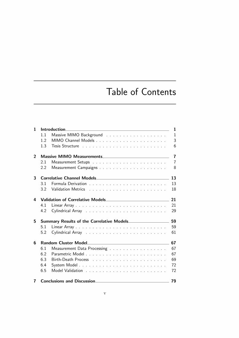
Table of Contents
1 Introduction 11.1 Massive MIMO Background . . . . . . . . . . . . . . . . . . 11.2 MIMO Channel Models . . . . . . . . . . . . . . . . . . . . . 31.3 Tesis Structure . . . . . . . . . . . . . . . . . . . . . . . . . 6
2 Massive MIMO Measurements 72.1 Measurement Setups . . . . . . . . . . . . . . . . . . . . . . 72.2 Measurement Campaigns . . . . . . . . . . . . . . . . . . . . 8
3 Correlative Channel Models 133.1 Formula Derivation . . . . . . . . . . . . . . . . . . . . . . . 133.2 Validation Metrics . . . . . . . . . . . . . . . . . . . . . . . 18
4 Validation of Correlative Models 214.1 Linear Array . . . . . . . . . . . . . . . . . . . . . . . . . . . 214.2 Cylindrical Array . . . . . . . . . . . . . . . . . . . . . . . . 29
5 Summary Results of the Correlative Models 595.1 Linear Array . . . . . . . . . . . . . . . . . . . . . . . . . . . 595.2 Cylindrical Array . . . . . . . . . . . . . . . . . . . . . . . . 61
6 Random Cluster Model 676.1 Measurement Data Processing . . . . . . . . . . . . . . . . . 676.2 Parametric Model . . . . . . . . . . . . . . . . . . . . . . . . 676.3 Birth-Death Process . . . . . . . . . . . . . . . . . . . . . . 696.4 System Model . . . . . . . . . . . . . . . . . . . . . . . . . . 726.5 Model Validation . . . . . . . . . . . . . . . . . . . . . . . . 72
7 Conclusions and Discussion 79
v

References 81
List of Figures 83
List of Tables 91
List of Abbreviations 95
vi
Chapter 1
Introduction
1.1 Massive MIMO Background
With the development of wireless communication systems, the demands forhigh data rate and link reliability of the communication systems also in-crease. One of the trends is going from single antenna to multiple antennas,so called multiple-input multiple-output (MIMO) [1]. Because of its advan-tages in terms of improved capacity and link reliability, MIMO technologyhas been widely studied in the past and used in various standards suchas Universal Mobile Telecommunication System (UMTS) and Long TermEvolution (LTE) [2].
The first studies were focused on point-to-point MIMO links, which iscalled conventional MIMO. In conventional MIMO where two devices trans-mit and receive with a relatively small number of antennas, each transmitantenna will be deployed with one transmit RF chain [3]. In recent years,the focus has shifted to conventional multi-user MIMO (MU-MIMO) wherea base station (BS) equipped with multiple antennas simultaneously servesmultiple single-antenna users and thereby achieves multiplexing gain. Thisway offers some big advantages over conventional point-to-point MIMO:user terminals can work with cheap single-antenna transceivers and mostof the expensive equipment can be placed at the BS. Another importantadvantage of MU-MIMO is their ability to achieve diversity, which makesthe performance of the system become more robust to the propagation en-vironment. Because of these advantages, MU-MIMO is progressively beingemployed throughout the world and has developed as a part of communi-cations standards, such as LTE, 802.11 (WiFi) and 802.16 (WiMAX).
In the next generation cellular networks, higher user densities and in-creased data rates are required. Due to the BS typically employs a fewantennas for most regular MU-MIMO systems, it limits the experiencedincrease of data rates and thereby the achieved spectral efficiencies. Re-
1

2 Introduction
searchers are thinking of increasing the number of antennas at the BS toboost the system performance.
The deployment of conventional MU-MIMO systems with a large num-ber of (tens to hundreds) antennas at the BS is known as massive MIMO inthe literature [4]. It is an emerging technology and has attracted significantattention in the research community due to the following main advantages:
• Spectral efficiency: It has been shown that massive MIMO is agood technology for enhancing spectral efficiency (bit/s/Hz/cell).This is achieved by massive arrays and simultaneous beamformingto users so that the received multipath components of the wantedsignal adds up coherently while the remaining part of the signal doesnot. Together the antenna elements can achieve unprecedented arraygains and spatial resolution, which will result in robustness to inter-user interference and increase the number of simultaneously servedusers per cell. Compared to a single-antenna system, massive MIMOis assumed to improve spectral efficiency by at least an order of mag-nitude [5–7].
• Interference reduction: The interference from other co-channelusers may significantly degrade the performance of a targeted user.Massive MIMO tackles this question by using interference reductionor cancellation techniques, such as dirty paper coding (DPC) forthe downlink and maximum likelihood (ML) multiuser detection forthe uplink. However, these technques are complex and suffer highcomputational complexity. [8]
• Transmit-Power efficiency: The massive MIMO technology de-scribed in [9] improves transmit-power efficiency due to diversity ef-fects and array gains. The power scaling law for massive MIMOsystems has been derived in [10]. It shows that, to achieve the per-formance equal to a single-input single-output (SISO) system, thetransmit power of each single-antenna user in a massive MIMO sys-tem can be scaled down proportionally to the number of BS antennasif the BS acquires perfect channel state information (CSI) or to thesquare root of the number of BS antennas if the BS has imperfectCSI [10]. This is the one of the important advantage of massiveMIMO and the potential for improving transmit-power efficiency ishuge.
• Link reliability: It is conceivable that a large number of degrees offreedom can be provided by the propagation channel due to the num-ber of antennas at the transmitter and receiver is typically assumed
Introduction 3
to be larger. The more degrees of freedom the better link reliabilityand the higher data rate [11].
With the above advantages, massive MIMO systems is widely consid-ered as a promising enabler for the 5G mobile communications.
1.2 MIMO Channel Models
In most cases, MIMO channels leads to the increased capacity comparedto SISO channels due to the assumption that the MIMO paths are uncor-related. The assumption has been flattened in [12]. It also has shown thatthe capacity of a measured channel is commonly less than the limit accord-ing to the environment. Since channel model is the deterministic portionof the whole system and their performance depends on the environment,accurate models are highly needed.
In general, there are two purposes served by MIMO channel models. Inthe first place, the models play as a channel simulator. A MIMO system canbe designed by employing a MIMO channel model in terms of the design forsignalling schemes, detection schemes and space-time codes. As a result,the same model can be applied to evaluate properly the performance of agiven system and build exemplar channels. In the second place, an accuratechannel model results in a relatively deep insight into the underlying physicsof the channel. It not only is good for the behaviour of a given channelanalysis, but also makes safe assumptions in system design.
To characterize massive MIMO channels and to evaluate system per-formance, it is important to develop an accurate model for it. Here, westudy two classes of MIMO channel models, correlative models and clustermodel, by using the measured channel data. The measurements for massiveMIMO will be briefly introduced in the Chapter 2.
1.2.1 Correlative Models
Various correlative models have been proposed for MIMO such as the Kro-necker, Weichselberger and Structured models. We focus on the first twomodels in this thesis.
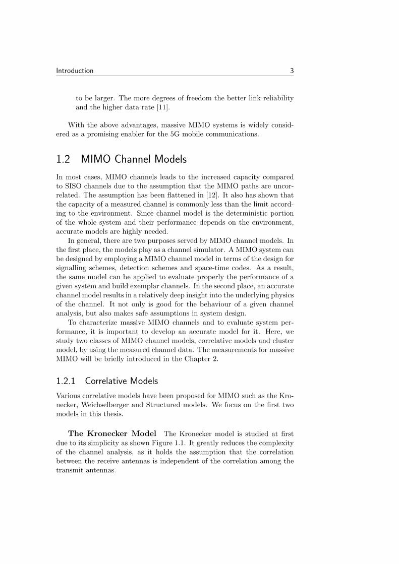
The Kronecker Model The Kronecker model is studied at firstdue to its simplicity as shown Figure 1.1. It greatly reduces the complexityof the channel analysis, as it holds the assumption that the correlationbetween the receive antennas is independent of the correlation among thetransmit antennas.
4 Introduction
Figure 1.1: Transmit correlation only depends on the scattering at the transmitside, and correspondingly, receive correlation only relies on the scattering atthe receive side.
In our work, the main task is to model the spatial correlation betweenmassive MIMO sub-channels within the framework of the Kronecker modelwithout the impact of antenna coupling. The massive MIMO channel modeltakes into account the correlation by treating the fixed correlation at thereceiver and transmitter following the well-known Kronecker model givenby [13]
Hkron = R1/2Rx GR
1/2Tx (1.1)
where the channel matrix G is populated with independent and identically
distributed (i.i.d.) zero-mean complex-Gaussian entries. The R1/2Rx and
R1/2Tx are the matrix square-roots of the receive-correlation matrix RRx and
the transmit-correlation matrix RTx, respectively.
The advantage of the Kronecker model is its simplicity, and it is oftenused for analytical study of MIMO systems. However, due to the assump-tion of no coupling between the transmit and receive sides, the model maynot be accurate enough for some propagation environments.
The Weichselberger Model A relatively more complex correla-tive model, i.e., the Weichselberger model, can be more accurate than theKronecker model as it introduces coupling effect between the propagationat the transmit and receive sides [14, 15]. The model can be representedin [15] as follows:
Hweich = URx(ΩΩΩG)UTTx (1.2)
where G denotes a random matrix with i.i.d complex-Gaussian entries. URx
and UTx are the one-sided eigenvectors. is the element-wise product oftwo matrices (or the Hadamard product), and ΩΩΩ is the element-wise squareroot of the power coupling matrix ΩΩΩ.
Introduction 5
The Weichselberger model suggests the opposite assumption relative tothe Kronecher model [14]; scatters at the two link ends cannot be consideredindependent and are coupled in some way. Because of this reason, theWeichselberger model is more accurate, when compared with the Kroneckermodel. However, additional complexity is required to define the powercoupling matrix.
1.2.2 Cluster Models
Cluster models, usually geometry-based, are based on the concept of clus-ters. A cluster is defined as a group of multipath components (MPCs) withsimilar parameters, such as angles of arrival (AOA), angles of departure(AOD) and delays. Cluster models simulate channels based on clustersthrough a set of stochastic parameter. One significant difference betweenthe cluster-based models and the correlatives models is that cluster modelscapture the time-variant nature of the radio channel. The most well-knowncluster models are the Saleh-Valenzuela model, the 3GPP Spatial Chan-nel Model (SCM), the Wireless World Initiative New Radio II (WINNERII) channel model, the COST 273 Model and the Random Cluster Model(RCM). In this thesis, we focus on the RCM. [13]
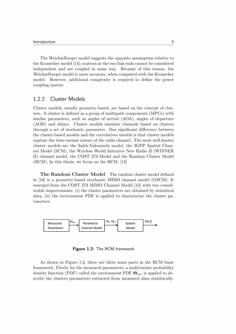
The Random Cluster Model The random cluster model definedin [16] is a geometry-based stochastic MIMO channel model (GSCM). Itemerged from the COST 273 MIMO Channel Model [13] with two consid-erable improvements: (i) the cluster parameters are obtained by statisticaldata, (ii) the environment PDF is applied to characterize the cluster pa-rameters.
Figure 1.2: The RCM framework
As shown in Figure 1.2, there are three main parts in the RCM basicframework. Firstly for the measured parameters, a multivariate probabilitydensity function (PDF) called the environment PDF Θenv is applied to de-scribe the clusters parameters extracted from measured data statistically.

6 Introduction
Next, in the parametric channel model, we use the obtained Θenv to gen-erate the cluster parameter sets Θc and multipath component parametersets Θc,p. With the parameters obtained from the environment PDF Θenv,channel matrices can be generated through the system model.
For the RCM, one of the greatest strengths is that a time-variant chan-nel is simulated by tracking the clusters over time domain. Secondly, themodel is simplified by using the environment PDF to characterize the chan-nels. However, the process of computing the environment PDF is intricate.How to define and clustering the clusters from the measurement data stillneed to be optimized.
1.3 Tesis Structure
In this thesis, based on real-life channel data, we investigate the suitabilityof three channel models for massive MIMO, e.g., the Kronecker model,the Weichselberger model, and the RCM. In order to validate the studiedchannel models and compare with the measured massive MIMO channels,on one hand, we evaluate the Kronecker model and the Weichselbergermodel by comparing the uplink capacity, zero-forcing (ZF) sum-rate andthe singular value to the measured channel; on the other hand, we validatethe correlation properties and channel fading process for both the RCMand measured channel.
This thesis report is organised as follows: Chapter 2 will give thedescription of four measurement campaigns for massive MIMO channels,based which we construct and validate the above-mentioned models. InChapter 3, the formula deviation for the correlative models and severalperformance metrics will be presented. The validation results and analysisfor the correlative models will be shown in Chapter 4 and Chapter 5. InChapter 6, the process of establishing the RCM will be described in detail,and the validation results in terms of spatial correlation and large-scalefading properties will be reported. Chapter 7 will give conclusions anddiscussion for this thesis work.
Chapter 2
Massive MIMO Measurements
As mentioned previously, the channel models constructed in this thesisare based on real environment channel measurements. For the massiveMIMO measurement campaigns, the measurement setups, the measurementenvironments as well as the measurement scenarios will be presented in thischapter. The selected measurement campaigns have been first reportedin [17–19], here gives a brief description, which is focused on their majorparameters.
2.1 Measurement Setups
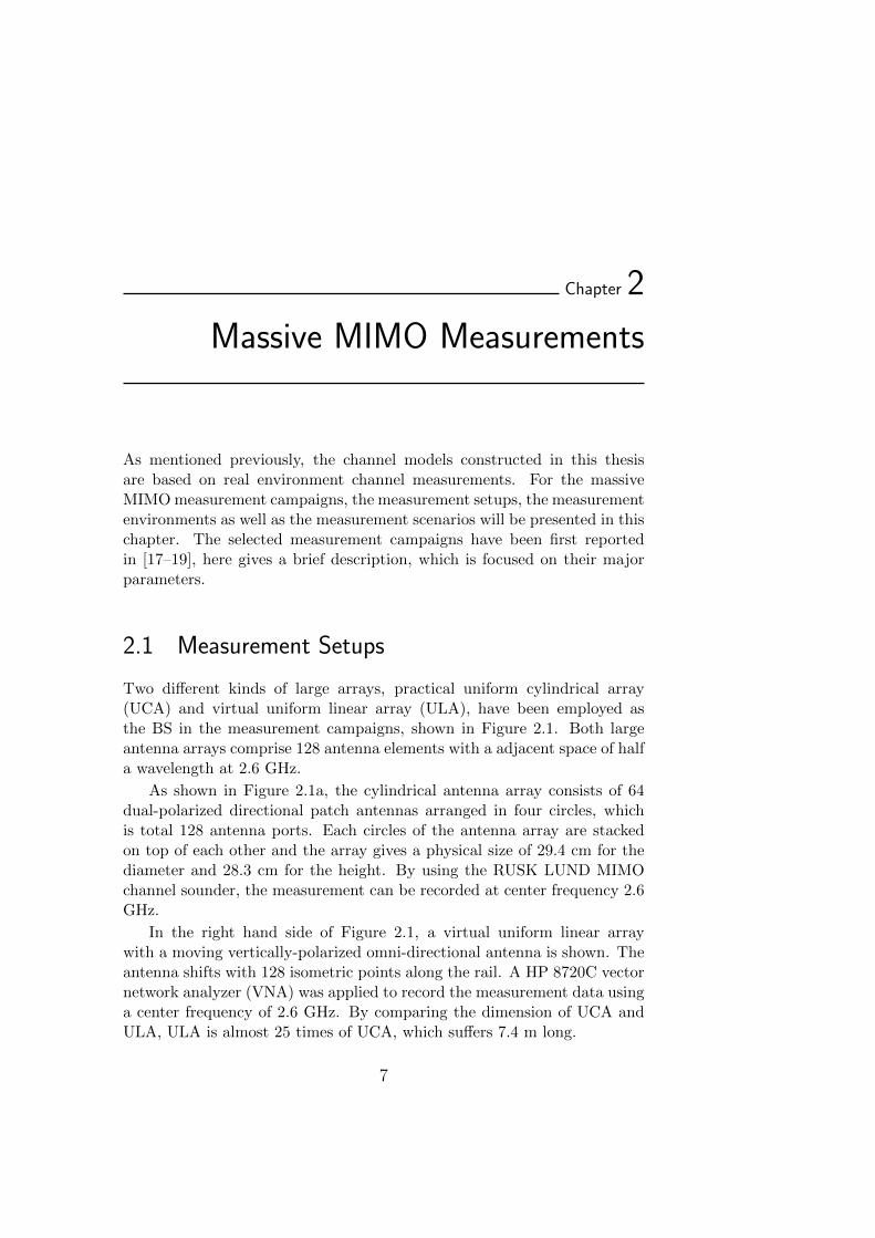
Two different kinds of large arrays, practical uniform cylindrical array(UCA) and virtual uniform linear array (ULA), have been employed asthe BS in the measurement campaigns, shown in Figure 2.1. Both largeantenna arrays comprise 128 antenna elements with a adjacent space of halfa wavelength at 2.6 GHz.
As shown in Figure 2.1a, the cylindrical antenna array consists of 64dual-polarized directional patch antennas arranged in four circles, whichis total 128 antenna ports. Each circles of the antenna array are stackedon top of each other and the array gives a physical size of 29.4 cm for thediameter and 28.3 cm for the height. By using the RUSK LUND MIMOchannel sounder, the measurement can be recorded at center frequency 2.6GHz.
In the right hand side of Figure 2.1, a virtual uniform linear arraywith a moving vertically-polarized omni-directional antenna is shown. Theantenna shifts with 128 isometric points along the rail. A HP 8720C vectornetwork analyzer (VNA) was applied to record the measurement data usinga center frequency of 2.6 GHz. By comparing the dimension of UCA andULA, ULA is almost 25 times of UCA, which suffers 7.4 m long.
7
8 Massive MIMO Measurements
a) Cylindrical array b) Linear array
Figure 2.1: Two large antenna arrays: a) practical uniform cylindrical array(UCA), and b) virtual uniform linear array (ULA).
2.2 Measurement Campaigns
The channel measurement campaigns were took place at the campus ofthe Faculty of Engineering (LTH), Lund University, Sweden (55.711510 N,13.210405 E). Four massive MIMO measurement campaigns are selectedto represent both the virtual user and the fully-synchronous user, and alsothe measurement environment of indoor and outdoor, namely the ”ULAwith 5 virtual users”, the ”UCA with 5 virtual users”, the ”UCA with 9synchronized users - outdoor”, and the ”UCA with 9 synchronized users -indoor”.
2.2.1 ULA with 5 Virtual Users
In this scenario, the user side equipped an omni-directional antenna withvertical polarization as the receiver. And the ULA at the BS was placedat the roof of E-building of LTH, which plays the role of transmitter. Themeasurement campaign was processed during the night aiming to get astatic channel.
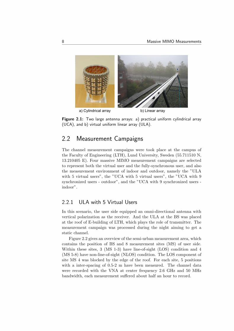
Figure 2.2 gives an overview of the semi-urban measurement area, whichcontains the position of BS and 8 measurement sites (MS) of user side.Within these sites, 3 (MS 1-3) have line-of-sight (LOS) condition and 4(MS 5-8) have non-line-of-sight (NLOS) condition. The LOS component ofsite MS 4 was blocked by the edge of the roof. For each site, 5 positionswith a inter-spacing of 0.5-2 m have been measured. The channel datawere recorded with the VNA at center frequency 2.6 GHz and 50 MHzbandwidth, each measurement suffered about half an hour to record.
Massive MIMO Measurements 9
Figure 2.2: Overview of the measurement area at the campus of the Facultyof Engineering (LTH), Lund University, Sweden. Two BS large antenna arrayswere placed at the same roof of E-building of LTH during the two respectivemeasurement campaigns, 8 MS sites were measured.
2.2.2 UCA with 5 Virtual Users
This scenario gives similar setup with the former scenario, an omni-directionalantenna with vertical polarization was deployed at the user side as the re-ceiver. The UCA, which is the BS, placed at the same roof of E-building ofLTH as ULA. Due to its compactness, the UCA was placed at the beginningof the ULA, shown in the top left corner of Figure 2.2.
The user (an omni-directional antenna) moved around the 8 user sites(MS 1-8) , four of the sites (MS 1-4) have LOS condition, while the otherfour (MS 5-8) have NLOS condition. 40 positions were measured with ainter-spacing of 0.5 m, and the data were recorded by the RUSK LUNDMIMO channel sounder at center frequency 2.6 GHz and 50 MHz band-width.
2.2.3 UCA with 9 Synchronized Users - Outdoor
In this measurement campaign, nine vertically-polarized omni-directionalantennas performed as nine simultaneous users. At the BS side, a UCAwas installed at the low roof (two floors) of E-building of LTH. Duringthe measurement, the 9 users were moving randomly inside a circle witha 5 m diameter, at a speed of about 0.5 m/s (see Figure 2.3b). To getboth vertical and horizontal polarizations, the users were asked to hold the

10 Massive MIMO Measurements
BS BS MS 1MS 1
MS 2MS 2
MS 3MS 3
MS 4MS 4
5 m
Measurement site (MS)
LOS scenario
NLOS scenario
(a) (b)
Figure 2.3: UCA with 9 synchronized users - outdoor measurement (a) Themeasurement area, (b) The users moving randomly in a 5 m diameter circle.
antennas with a angle of inclination (45 degrees). Except the non-crowdcondition, the heavy crowd condition with 10 - 12 persons walking aroundthe 9 users in the circle has also been considered. [20]
As shown in Figure 2.3a, the BS location and 4 sites with differentpropagation conditions of user side (MS 1-4) were labeled. MS 1 and MS2 have LOS condition, MS 3 and MS 4 have NLOS condition. The RUSKLUND MIMO channel sounder was connected to record the measurementdata at 2.6 GHz center frequency and 40 MHz bandwidth. At each mea-surement, 300 snapshots were recorded during a measurement period of 17seconds. [19]
2.2.4 UCA with 9 Synchronized Users - Indoor
This measurement were performed in an auditorium of E-building of LTH,which represents a indoor duplicate scenario of the ”UCA with 9 synchro-nized users - outdoor” scenario. The cylindrical array at the BS side wasfixed at a height of 3.2 m. For the user side, 9 users were sited randomlyin 20 seats. Each of them held a vertically-polarized omni-directional an-tenna either vertically or tilted 45 degrees during different measurements,and the users were asked to move the antenna arbitrary with a speed lessthan 0.5 m/s. Besides including the non-crowd case with only 9 active userssitting among the 20 seats, the heavy crowded condition were performedwith additional 11 non-active users to fill the 20 seats (see Figure 2.4b).
Figure 2.4a shows an overview of the measurement area. 4 BS positionsand 2 groups of users in both middle and back of the auditorium have been

Massive MIMO Measurements 11
measured respectively. The channel sounder named RUSK LUND MIMOwas appointed to record the measurement data followed the conditions,which are 2.6 GHz center frequency and 40 MHz bandwidth. In order torecord each measurement, 300 snapshots were recorded within the periodof 17 seconds.
(a) (b)
Figure 2.4: UCA with 9 synchronized users - indoor measurement (a) Themeasurement area, (b) The users.

12 Massive MIMO Measurements

Chapter 3
Correlative Channel Models
3.1 Formula Derivation
It is important to highlight the significant drawback of the full correla-tion matrix, which is the huge size of parameters. The correlative channelmodels, the Kronecker and Weichselberger, overcome the drawback by de-composing the full correlation using the parameterized one-sided correlationmatrices.
The Kronecker modelFor the massive MIMO measurement, the narrowband channel gain matrixH`,n is given by the Equation 3.1 for convenience of presentation. The H`,n
is the channel matrix at subcarrier ` and snapshot n, that is
H`,n =
h11 · · · h1M...
. . ....
hK1 · · · hKM
(3.1)
According to the definition in [21], the covariance of the channel can beformulated using the measured channel matrix as
RH,` = Evec(H`)vec(H`)H (3.2)
where RH,` ∈ CK×M is a positive semi-definite (PSD) Hermitian matrix,vec(H`) is to stack H` into a vector columnwise, and (.)H stands for con-jugate transpose operation.
The Kronecker model assumes that the separate spatial correlationstructure at the transmitter and receiver sides can be described by thetransmit-correlation and receive-correlation matrices. It means that thetwo correlation matrices are not coupled in any cases. As mentioned in [13],
13
14 Correlative Channel Models
the narrowband receive-correlation matrix RRx ∈ CK×K can be achieved asfollows
RRx,` =1
N
N∑n=1
Hn,`HHn,`
= EH`HH` (3.3)
The narrowband transmit-correlation matrix RTx ∈ CM×M is achieved asEquation 3.4
RTx,` =1
N
N∑n=1
HTn,`H
∗n,`
= EHH` H`T (3.4)
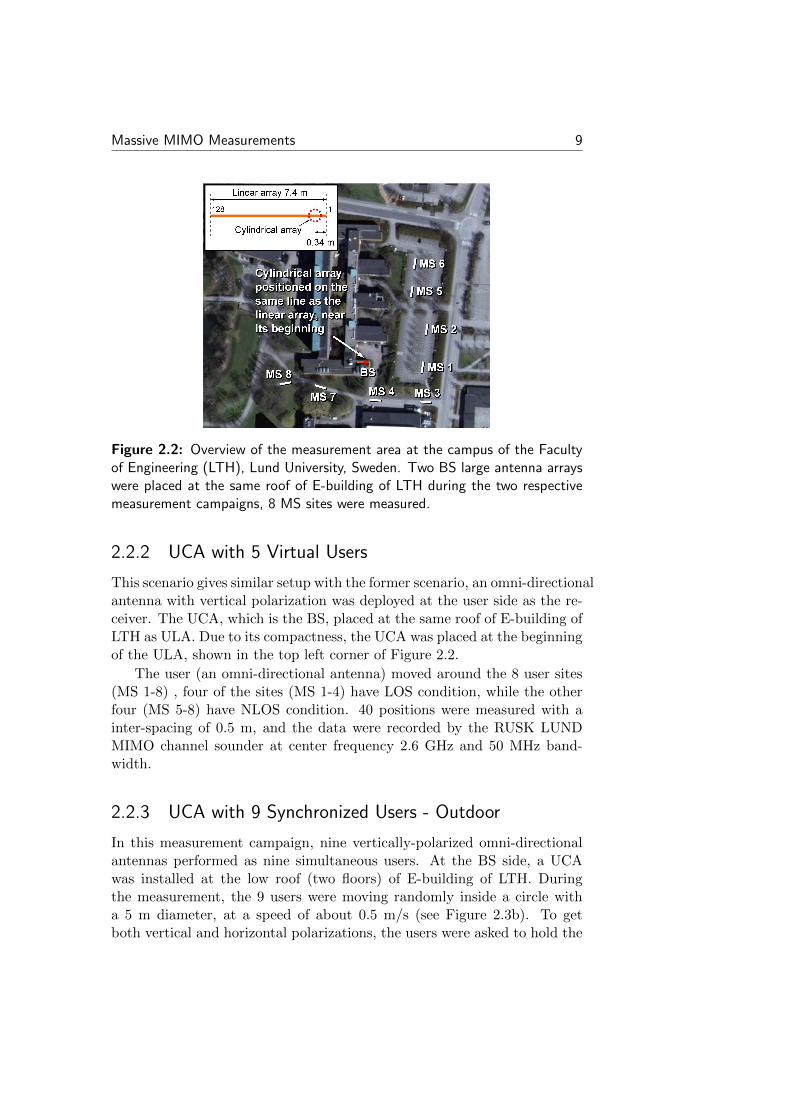
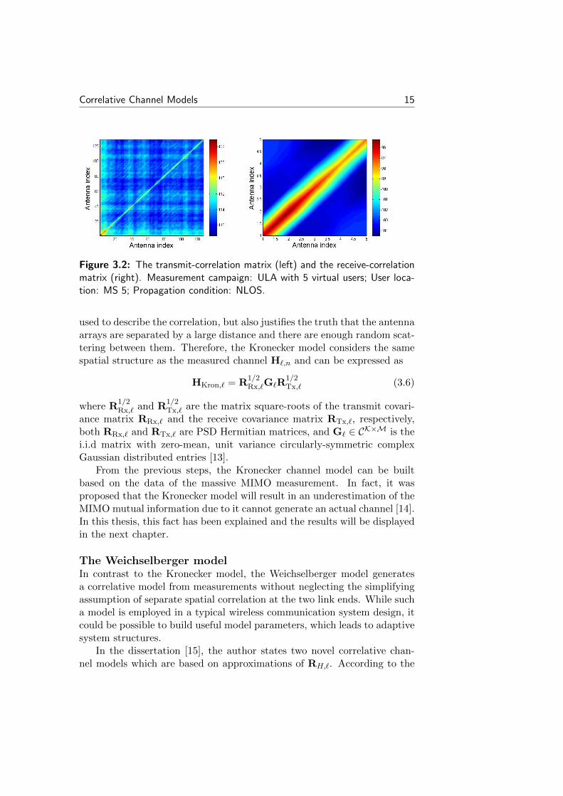
Figure 3.1: The transmit-correlation matrix (left) and the receive-correlationmatrix (right). Measurement campaign: ULA with 5 virtual users; User loca-tion: MS 2; Propagation condition: LOS.
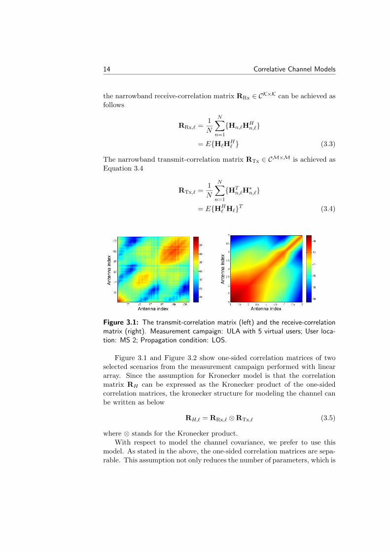
Figure 3.1 and Figure 3.2 show one-sided correlation matrices of twoselected scenarios from the measurement campaign performed with lineararray. Since the assumption for Kronecker model is that the correlationmatrix RH can be expressed as the Kronecker product of the one-sidedcorrelation matrices, the kronecker structure for modeling the channel canbe written as below
RH,` = RRx,` ⊗RTx,` (3.5)
where ⊗ stands for the Kronecker product.With respect to model the channel covariance, we prefer to use this
model. As stated in the above, the one-sided correlation matrices are sepa-rable. This assumption not only reduces the number of parameters, which is
Correlative Channel Models 15
Figure 3.2: The transmit-correlation matrix (left) and the receive-correlationmatrix (right). Measurement campaign: ULA with 5 virtual users; User loca-tion: MS 5; Propagation condition: NLOS.
used to describe the correlation, but also justifies the truth that the antennaarrays are separated by a large distance and there are enough random scat-tering between them. Therefore, the Kronecker model considers the samespatial structure as the measured channel H`,n and can be expressed as
HKron,` = R1/2Rx,`G`R
1/2Tx,` (3.6)
where R1/2Rx,` and R
1/2Tx,` are the matrix square-roots of the transmit covari-
ance matrix RRx,` and the receive covariance matrix RTx,`, respectively,both RRx,` and RTx,` are PSD Hermitian matrices, and G` ∈ CK×M is thei.i.d matrix with zero-mean, unit variance circularly-symmetric complexGaussian distributed entries [13].
From the previous steps, the Kronecker channel model can be builtbased on the data of the massive MIMO measurement. In fact, it wasproposed that the Kronecker model will result in an underestimation of theMIMO mutual information due to it cannot generate an actual channel [14].In this thesis, this fact has been explained and the results will be displayedin the next chapter.
The Weichselberger modelIn contrast to the Kronecker model, the Weichselberger model generatesa correlative model from measurements without neglecting the simplifyingassumption of separate spatial correlation at the two link ends. While sucha model is employed in a typical wireless communication system design, itcould be possible to build useful model parameters, which leads to adaptivesystem structures.
In the dissertation [15], the author states two novel correlative chan-nel models which are based on approximations of RH,`. According to the

16 Correlative Channel Models
concept of the vector modes in his thesis, the first channel model can bedefined. Another popular version is based on the novel concept, namedstructured modes. The last model is presented in many literatures, and itwill be viewed as the Weichselberger model in the following derivations.
Since the Weichselberger model takes into account the joint spatialstructure and describes the MIMO propagation channel using the one-sidedcorrelation matrices, it is a novel MIMO propagation channel model. Theeigenbases of the one-side correlation matrices are the same as in the Kro-necker model and they are coupled with coupling matrix.
Consider the narrowband channel matrix H`,n, the Eigen-value decom-position(EVD) of the correlation matrix RH,` is generated because it isPSD Hermitian symmetric and presented through the following equation.
RH,` =
KM∑i=1
λH,iuH,iuHH,i
= UH,`ΛH,`UHH,` (3.7)
where UH,` is the spatial eigenbases of the full channel correlation matrix,which is unitary matrix, and ΛH,` is diagonal matrix composed with theeigen values of RH,`.
As stated in the Kronecker model, the one-sided correlation matricesare Hermitian, so it can be decomposed by using EVD, formulated as
RRx,` =
K∑k=1
λRx,kuRx,kuHRx,k
= URx,`ΛRx,`UHRx,` (3.8)
RTx,` =
M∑m=1
λTx,muTx,muHTx,m
= UTx,`ΛTx,`UHTx,` (3.9)
where λRx,k and λTx,m are the eigenvalues for the receive-correlation matrixand the transmit-correlation matrix, uRx,k and uTx,m are the receive andtransit eigenvectors, and URx,` and UTx,` are the receive and transmiteigenbases, respectively. Also, uRx,k and uTx,m are referred to as the one-sided eigenvectors, URx,` and UTx,` are called as the one-sided eigenbases.
Given the eigenbases of the full channel correlation matrix, it can berecast in terms of the eigenbasis at the receiver and transmitter as follows:
UH,` = URx,` ⊗UTx,` (3.10)
Correlative Channel Models 17
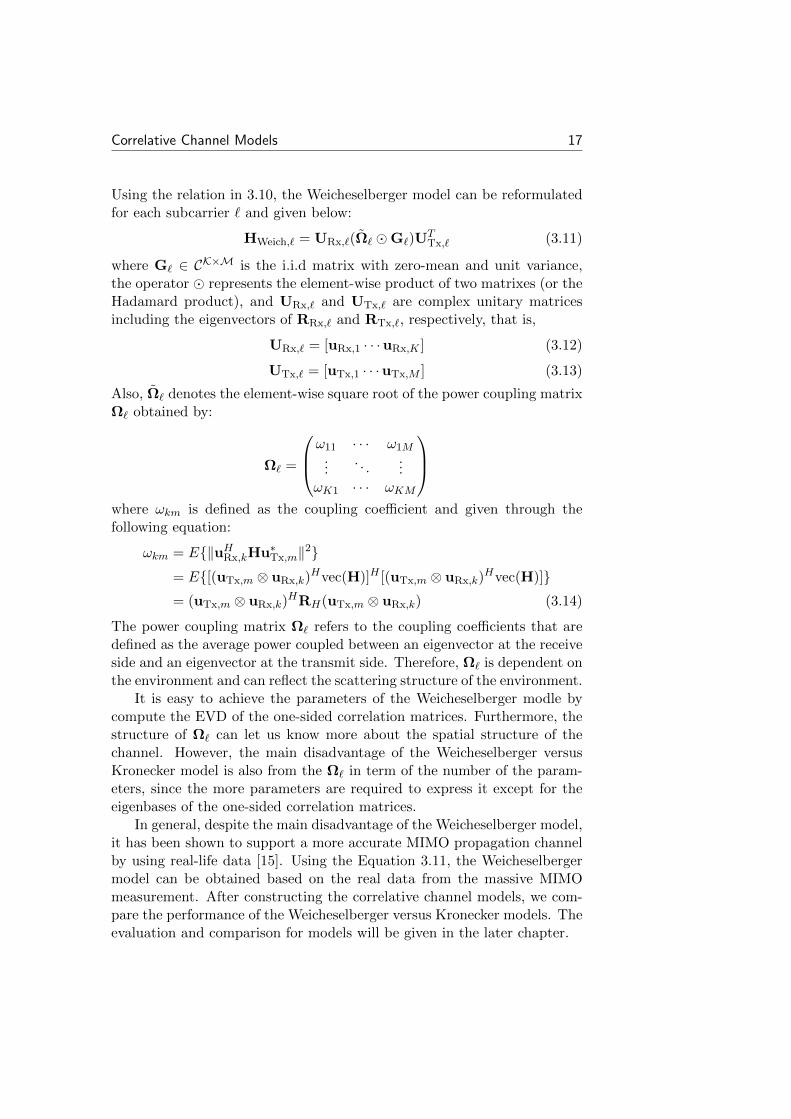
Using the relation in 3.10, the Weicheselberger model can be reformulatedfor each subcarrier ` and given below:
HWeich,` = URx,`(Ω` G`)UTTx,` (3.11)
where G` ∈ CK×M is the i.i.d matrix with zero-mean and unit variance,the operator represents the element-wise product of two matrixes (or theHadamard product), and URx,` and UTx,` are complex unitary matricesincluding the eigenvectors of RRx,` and RTx,`, respectively, that is,
URx,` = [uRx,1 · · ·uRx,K ] (3.12)
UTx,` = [uTx,1 · · ·uTx,M ] (3.13)
Also, Ω` denotes the element-wise square root of the power coupling matrixΩ` obtained by:
Ω` =
ω11 · · · ω1M...
. . ....
ωK1 · · · ωKM
where ωkm is defined as the coupling coefficient and given through thefollowing equation:
ωkm = E‖uHRx,kHu∗Tx,m‖2= E[(uTx,m ⊗ uRx,k)
Hvec(H)]H [(uTx,m ⊗ uRx,k)Hvec(H)]
= (uTx,m ⊗ uRx,k)HRH(uTx,m ⊗ uRx,k) (3.14)
The power coupling matrix Ω` refers to the coupling coefficients that aredefined as the average power coupled between an eigenvector at the receiveside and an eigenvector at the transmit side. Therefore, Ω` is dependent onthe environment and can reflect the scattering structure of the environment.
It is easy to achieve the parameters of the Weicheselberger modle bycompute the EVD of the one-sided correlation matrices. Furthermore, thestructure of Ω` can let us know more about the spatial structure of thechannel. However, the main disadvantage of the Weicheselberger versusKronecker model is also from the Ω` in term of the number of the param-eters, since the more parameters are required to express it except for theeigenbases of the one-sided correlation matrices.
In general, despite the main disadvantage of the Weicheselberger model,it has been shown to support a more accurate MIMO propagation channelby using real-life data [15]. Using the Equation 3.11, the Weicheselbergermodel can be obtained based on the real data from the massive MIMOmeasurement. After constructing the correlative channel models, we com-pare the performance of the Weicheselberger versus Kronecker models. Theevaluation and comparison for models will be given in the later chapter.
18 Correlative Channel Models
3.2 Validation Metrics
In this section, a few metrics used in the literature are employed to verify theperformance of channel models. Each metric is provided an interpretationand examines a different aspect of the model. Thesis metrics are used incomparing the correlative models’ ability to predict the measured channelsfor our work, which give us absolute references.
3.2.1 System Model
Consider the uplink transmission of a single-cell MU-MIMO channel systemwith M antennas at the BS and K single-antenna users (K ≤ M). Orthog-onal frequency division multiplexing(OFDM) with L subcarriers is used toreduce the correlation in the user sides. The communication between theBS and the users takes place in the subcarriers L and snapshots N. Thechannel input-output relationship is given at subcarrier ` and snapshot n,that is
y`,n =
√P
MH`,nx`,n + w`,n (3.15)
Where H`,n ∈ CM×K represents the channel matrix between the BS andthe users; y`,n ∈ CM×1 and x`,n ∈ CK×1 are the output and input vectors,
respectively and w`,n ∈ CM×1 is the noise vector at the receiver whoseelements are i.i.d with zero mean and unit variance; P is the total transmitpower and P
M refers to the average transmitted power.
3.2.2 Normalization
With the Equation 3.15 proposed, it is easy to achieve the instantaneoussignal to noise ratio (SNR) per receive antenna, which results in averagedover all receive antennas, that is given by
ρ =P
σ2w
‖H`,n‖2FKM
(3.16)
where σ2w means the variance of the noise vector. However, it is assumedas 1 in our system in order to simplify the model.
For our simulation, the different MIMO systems and configurations suchas M = 128, 64 and 32 are used. Therefore, it is required to ensure a faircomparison of the capacity performance for the different configurations, andsince the total power P has been fixed, the solving strategy is to considerthe same receive SNR, as below:
Correlative Channel Models 19
Considering the measured channel matrix H`,n taken over all N mea-surement snapshots and L subcarriers, the normalized channel matrix canbe expressed as
Hnorm`,n =
√√√√√√KMLN
N∑n=1
L∑l=1
‖Hmeas`,n ‖2F
Hmeas`,n (3.17)
It is easily followed that
1
L
L∑`=1
1
N
N∑n=1
‖Hnormn,` ‖2F = KM (3.18)
In the Equation 3.17, the average of the Frobenius norm of the channelsnapshots and subcarriers are fixed, and the normalization can preserves therelative difference in the channel power over time-frequency resources, butkeep the average of the SNR at P
σ2w
(σ2w=1). These normalization can satisfy
a fair comparison, because the obtained average SNR from normalizationis equivalent to the average SNR of a SISO system with the same powerand noise power.
3.2.3 Uplink Capacity for MU-MIMO
For the uplink transmission of the MU-MIMO system, we assume the CSIis unknown by the transmitter, all users have the same transmit powerallocation. The uplink capacity at subcarrier ` is obtained in the unit ofbps/Hz as [22]
Cuplink,` = log2 det(IM +EsMN0
HH` H`) (3.19)
where IM is the identity matrix and H` is the channel response matrix atsubcarrier `. The average SNR, which denoted by Es
MN0, is decreased with
the increasing M thus the array gain can be obtained.
3.2.4 Zero-Forcing Pre-Coding Sum-Rate
The sum-rate of the MU-MIMO uplink can be achieved by the ZF pre-coding scheme, which is one of the most popular linear pre-coding tech-niques, aiming to remove the ISI (Inter-Symbol Interference). The ZFpre-coder can be written as
WZF = (H∗HT )−1H∗ (3.20)
20 Correlative Channel Models
By computing WZF into the the signal model, the sum-rate capacity of ZFpre-coding becomes
CZF,` =
K∑i=1
log2(1 +EsM
N0[(H∗`H
T` )−1]ii
) (3.21)
where EsM is the signal power of ith user, and N0[(H
∗`H
T` )−1]ii is the noise
power of ith user.
3.2.5 Singular Value Spread
This section presents another performance metric to analysis the massiveMIMO radio channel, singular value spread (also known as the conditionnumber). The channel matrix H has a singular value decomposition:
H = UΣVH (3.22)
where U ∈ CK×K and V ∈ CM×M are unitary matrices. The diagonalmatrix Σ ∈ CK×M is composed by the singular values σ1, σ2, · · · , σk, thesingular value spread κ is defined as:
κ =σmax
σmin(3.23)
where σmax and σmin are the maximal and minimal singular values, respec-tively. The κ (1 ≤ κ ≤ ∞) is the ratio between σmax and σmin, where κ = 1indicates a orthogonal channel matrix, otherwise a large κ shows that atleast two rows of the H are similar, which means at least one of the K userswill not be served.
Chapter 4
Validation of Correlative Models
In the previous chapter, we have introduced the four measurement cam-paigns in order to support the measured data and discussed a few metricscommonly used to validate the performance of channel models. In thischapter, the selected measurement scenarios were collected in very differentenvironments, using two large antenna arrays whose specifications differ.
In order to determine the correlative models’ usefulness in massiveMIMO, three validation metrics uplink capacity, ZF sum-rate and singu-lar value are shown in the below sections for the selected measurementscenarios. The validation metrics give an accuracy with which a modelcharacterizes the massive MIMO channels, thus, we can use them to verifythe correlative models. Furthermore, we compare the metrics achieved inthe measured channels with those achieved in the correlative models ac-cording to different aspects, such as the propagation condition, i.e., LOSversus NLOS; propagation environment, i.e., indoor versus outdoor; theenvironment at user side, i.e., crowded versus non-crowded; and differentBS locations.
4.1 Linear Array
This section introduces the validation results of the correlative models,when chosen scenarios are gathered in the first measurement campaign(”ULA with 5 virtual users”). For the measured channels and the correla-tive models, the three validation metrics are shown on the order of 5, 32,64 and 128 antennas equipped at the BS.
4.1.1 Selection of Antennas
Different number of antennas at the BS gives different channel performance.Here, we describe the method of antenna selection in detail and try to cover
21
22 Validation of Correlative Models
all antennas on the array:
1. M = 128: All antennas on the array are used.
2. M = 64: The adjacent antenna sliding window with 64 antennasis selected to slide from the first antenna to the final one, whenconsidering the ULA. After that, there are 65 sliding windows forour selection in total. We do a simulation for each sliding window, sothe 65 simulation results are achieved to calculate the uplink capacity,ZF sum-rate and singular value, then the calculated parameters areaveraged over different simulations.
3. M = 32 and 5: Except for the sliding window size is 32 and 5 anten-nas, respectively, the same method is used as M =64.
4.1.2 ULA with 5 Virtual Users
To observe the performance of the correlative models in LOS and NLOSpropagation conditions, the measured data gathered in the following twoscenarios are used.
• The first scenario occurs in a LOS outdoor environment. The fiveusers are close to each other at MS 2, whereas the BS remains fixed.Details on the position information can be found in the Figure 2.2.In order to have the strongest LOS characteristic, we choose thisscenario to be investigated.
• The second scenario is the same outdoor environment as the firstscenario, however, the close five users are at MS 5 and communicatewith BS in a NLOS condition. This scenario is used because thereare rich scatterers between the user and the BS.
LOS Scenario
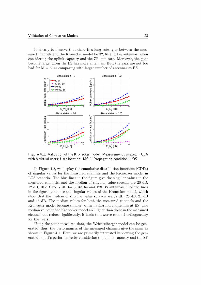
Figure 4.1 shows both the uplink capacity and the ZF sum-rate as a func-tion of Es/N0 (-10 to 10 dB) for different antenna deployments, when con-sidering the Kronecker model in LOS scenario. It can be known from thefigure that the uplink capacity for the measured channels and the Kroneckermodel increases as Es/N0 increases for 5, 32, 64 and 128 antennas, respec-tively. Furthermore, it also becomes larger, when increasing the number ofBS antennas. For the ZF sum-rate, it goes to larger value as a function ofthe number of BS antennas for the measured channels. However, for theKronecker model, it keeps in 0 [bps/Hz] expect for M = 128.
Validation of Correlative Models 23
It is easy to observe that there is a long rates gap between the mea-sured channels and the Kronecker model for 32, 64 and 128 antennas, whenconsidering the uplink capacity and the ZF sum-rate. Moreover, the gapsbecome large, when the BS has more antennas. But, the gaps are not toobad for M = 5, as comparing with larger number of antennas at BS.
−10 −5 0 5 100
5
10
15
20
Es/N
0 [dB]
Upl
ink
sum
−ra
te [b
ps/H
z]
Base station − 5
KronKron, ZFMeasMeas, ZF
−10 −5 0 5 100
5
10
15
20
Es/N
0 [dB]
Upl
ink
sum
−ra
te [b
ps/H
z]
Base station − 32
−10 −5 0 5 100
5
10
15
20
Es/N
0 [dB]
Upl
ink
sum
−ra
te [b
ps/H
z]
Base station − 64
−10 −5 0 5 100
5
10
15
20
Es/N
0 [dB]
Upl
ink
sum
−ra
te [b
ps/H
z]
Base station − 128
Figure 4.1: Validation of the Kronecker model. Measurement campaign: ULAwith 5 virtual users; User location: MS 2; Propagation condition: LOS.
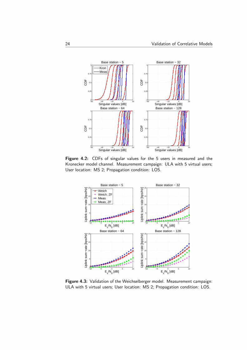
In Figure 4.2, we display the cumulative distribution functions (CDFs)of singular values for the measured channels and the Kronecker model inLOS scenario. The blue lines in the figure give the singular values in themeasured channels, and the median of singular value spreads are 20 dB,12 dB, 10 dB and 7 dB for 5, 32, 64 and 128 BS antennas. The red linesin the figure announce the singular values of the Kronecker model, whichshow that the median of singular value spreads are 37 dB, 23 dB, 21 dBand 16 dB. The median values for both the measured channels and theKronecker model become smaller, when having more antennas at BS. Themedian values in the Kronecker model are higher than those in the measuredchannel and reduce significantly, it leads to a worse channel orthogonalityfor the users.
Using the same measured data, the Weichselberger model can be gen-erated, thus, the performances of the measured channels give the same asshown in Figure 4.1. Here, we are primarily interested in viewing the gen-erated model’s performance by considering the uplink capacity and the ZF
24 Validation of Correlative Models
−60 −40 −20 0 200
0.25
0.5
0.75
1
Singular values [dB]
CD
F
Base station − 5
KronMeas
−60 −40 −20 0 200
0.25
0.5
0.75
1
Singular values [dB]
CD
F
Base station − 32
−60 −40 −20 0 200
0.25
0.5
0.75
1
Singular values [dB]
CD
F
Base station − 64
−60 −40 −20 0 200
0.25
0.5
0.75
1
Singular values [dB]
CD
F
Base station − 128
Figure 4.2: CDFs of singular values for the 5 users in measured and theKronecker model channel. Measurement campaign: ULA with 5 virtual users;User location: MS 2; Propagation condition: LOS.
−10 −5 0 5 100
5
10
15
20
Es/N
0 [dB]
Upl
ink
sum
−ra
te [b
ps/H
z]
Base station − 5
WeichWeich, ZFMeasMeas, ZF
−10 −5 0 5 100
5
10
15
20
Es/N
0 [dB]
Upl
ink
sum
−ra
te [b
ps/H
z]
Base station − 32
−10 −5 0 5 100
5
10
15
20
Es/N
0 [dB]
Upl
ink
sum
−ra
te [b
ps/H
z]
Base station − 64
−10 −5 0 5 100
5
10
15
20
Es/N
0 [dB]
Upl
ink
sum
−ra
te [b
ps/H
z]
Base station − 128
Figure 4.3: Validation of the Weichselberger model. Measurement campaign:ULA with 5 virtual users; User location: MS 2; Propagation condition: LOS.
Validation of Correlative Models 25
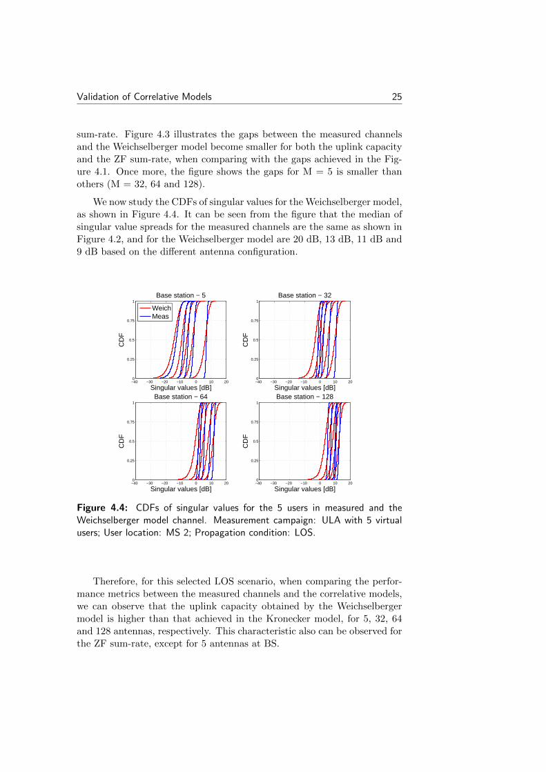
sum-rate. Figure 4.3 illustrates the gaps between the measured channelsand the Weichselberger model become smaller for both the uplink capacityand the ZF sum-rate, when comparing with the gaps achieved in the Fig-ure 4.1. Once more, the figure shows the gaps for M = 5 is smaller thanothers (M = 32, 64 and 128).
We now study the CDFs of singular values for the Weichselberger model,as shown in Figure 4.4. It can be seen from the figure that the median ofsingular value spreads for the measured channels are the same as shown inFigure 4.2, and for the Weichselberger model are 20 dB, 13 dB, 11 dB and9 dB based on the different antenna configuration.
−40 −30 −20 −10 0 10 200
0.25
0.5
0.75
1
Singular values [dB]
CD
F
Base station − 5
WeichMeas
−40 −30 −20 −10 0 10 200
0.25
0.5
0.75
1
Singular values [dB]
CD
F
Base station − 32
−40 −30 −20 −10 0 10 200
0.25
0.5
0.75
1
Singular values [dB]
CD
F
Base station − 64
−40 −30 −20 −10 0 10 200
0.25
0.5
0.75
1
Singular values [dB]
CD
F
Base station − 128
Figure 4.4: CDFs of singular values for the 5 users in measured and theWeichselberger model channel. Measurement campaign: ULA with 5 virtualusers; User location: MS 2; Propagation condition: LOS.
Therefore, for this selected LOS scenario, when comparing the perfor-mance metrics between the measured channels and the correlative models,we can observe that the uplink capacity obtained by the Weichselbergermodel is higher than that achieved in the Kronecker model, for 5, 32, 64and 128 antennas, respectively. This characteristic also can be observed forthe ZF sum-rate, except for 5 antennas at BS.
26 Validation of Correlative Models
NLOS Scenario
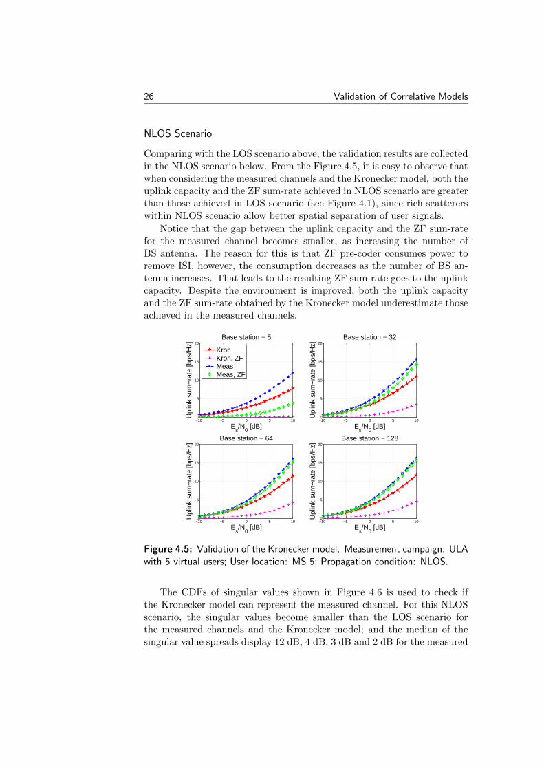
Comparing with the LOS scenario above, the validation results are collectedin the NLOS scenario below. From the Figure 4.5, it is easy to observe thatwhen considering the measured channels and the Kronecker model, both theuplink capacity and the ZF sum-rate achieved in NLOS scenario are greaterthan those achieved in LOS scenario (see Figure 4.1), since rich scattererswithin NLOS scenario allow better spatial separation of user signals.
Notice that the gap between the uplink capacity and the ZF sum-ratefor the measured channel becomes smaller, as increasing the number ofBS antenna. The reason for this is that ZF pre-coder consumes power toremove ISI, however, the consumption decreases as the number of BS an-tenna increases. That leads to the resulting ZF sum-rate goes to the uplinkcapacity. Despite the environment is improved, both the uplink capacityand the ZF sum-rate obtained by the Kronecker model underestimate thoseachieved in the measured channels.
−10 −5 0 5 100
5
10
15
20
Es/N
0 [dB]
Upl
ink
sum
−ra
te [b
ps/H
z]
Base station − 5
KronKron, ZFMeasMeas, ZF
−10 −5 0 5 100
5
10
15
20
Es/N
0 [dB]
Upl
ink
sum
−ra
te [b
ps/H
z]
Base station − 32
−10 −5 0 5 100
5
10
15
20
Es/N
0 [dB]
Upl
ink
sum
−ra
te [b
ps/H
z]
Base station − 64
−10 −5 0 5 100
5
10
15
20
Es/N
0 [dB]
Upl
ink
sum
−ra
te [b
ps/H
z]
Base station − 128
Figure 4.5: Validation of the Kronecker model. Measurement campaign: ULAwith 5 virtual users; User location: MS 5; Propagation condition: NLOS.
The CDFs of singular values shown in Figure 4.6 is used to check ifthe Kronecker model can represent the measured channel. For this NLOSscenario, the singular values become smaller than the LOS scenario forthe measured channels and the Kronecker model; and the median of thesingular value spreads display 12 dB, 4 dB, 3 dB and 2 dB for the measured

Validation of Correlative Models 27
channels, 24 dB, 12 dB, 11.5 dB and 11 dB for the Weichselberger model,for all cases of 5, 32, 64 and 128 antennas. Obviously the median values ofthe model are larger than the measured channels, so it is not a good modelto represent the measured channels.
−40 −30 −20 −10 0 10 200
0.25
0.5
0.75
1
Singular values [dB]
CD
F
Base station − 5
KronMeas
−40 −30 −20 −10 0 10 200
0.25
0.5
0.75
1
Singular values [dB]
CD
F
Base station − 32
−40 −30 −20 −10 0 10 200
0.25
0.5
0.75
1
Singular values [dB]
CD
F
Base station − 64
−40 −30 −20 −10 0 10 200
0.25
0.5
0.75
1
Singular values [dB]
CD
F
Base station − 128
Figure 4.6: CDFs of singular values for the 5 users in measured and theKronecker model channel. Measurement campaign: ULA with 5 virtual users;User location: MS 5; Propagation condition: NLOS.
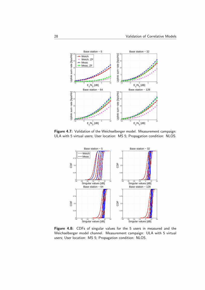
We now use measured data from NLOS scenario to generate the We-ichselberger model and describe its uplink capacity and ZF sum-rate whenusing different number of antennas, as shown in Figure 4.7. The Weichsel-berger model supports higher uplink capacity and ZF sum-rate than theKronecker model for 5, 32, 64 and 128 antennas in this NLOS scenario,when comparing with Figure 4.5. Because of this reason, the Weichsel-berger model is closer to the measured model than the Kronecker model.
In Figure 4.8, the median of singular value spreads are 13 dB, 7 dB, 6.5dB and 6 dB for equipping 5, 32, 64 and 128 antennas at the BS, respec-tively. Compare the CDF curves of singular values between the measuredchannels and the Weichselberger model, both singular values are close, how-ever, they also give some difference. Singular value spreads can reflect thebenefits of complex propagation. Both the measured channels and the We-ichselberger model have smaller singular value spreads. That indicates amuch better user channel orthogonality in the measured channels and themodel channels.
28 Validation of Correlative Models
−10 −5 0 5 100
5
10
15
20
Es/N
0 [dB]
Upl
ink
sum
−ra
te [b
ps/H
z]
Base station − 5
WeichWeich, ZFMeasMeas, ZF
−10 −5 0 5 100
5
10
15
20
Es/N
0 [dB]
Upl
ink
sum
−ra
te [b
ps/H
z]
Base station − 32
−10 −5 0 5 100
5
10
15
20
Es/N
0 [dB]
Upl
ink
sum
−ra
te [b
ps/H
z]
Base station − 64
−10 −5 0 5 100
5
10
15
20
Es/N
0 [dB]
Upl
ink
sum
−ra
te [b
ps/H
z]
Base station − 128
Figure 4.7: Validation of the Weichselberger model. Measurement campaign:ULA with 5 virtual users; User location: MS 5; Propagation condition: NLOS.
−40 −30 −20 −10 0 10 200
0.25
0.5
0.75
1
Singular values [dB]
CD
F
Base station − 5
WeichMeas
−40 −30 −20 −10 0 10 200
0.25
0.5
0.75
1
Singular values [dB]
CD
F
Base station − 32
−40 −30 −20 −10 0 10 200
0.25
0.5
0.75
1
Singular values [dB]
CD
F
Base station − 64
−40 −30 −20 −10 0 10 200
0.25
0.5
0.75
1
Singular values [dB]
CD
F
Base station − 128
Figure 4.8: CDFs of singular values for the 5 users in measured and theWeichselberger model channel. Measurement campaign: ULA with 5 virtualusers; User location: MS 5; Propagation condition: NLOS.
Validation of Correlative Models 29
Summarizing, we find that the Weichselberger model is more closerto the measured channels than the Kronecker model, when consideringthe LOS scenario and NLOS scenario, respectively. That is due to theseparability assumption for the Kronecker model that scatterers at bothsides can not be coupled. Furthermore, when considering the Kroneckermodel and the Weichselberger model, respectively, NLOS scenario withrich scatterers can bring the better benefits than the LOS scenario, sincescatterers in the environment can support strong decorrelation effect to thechannel.
4.2 Cylindrical Array
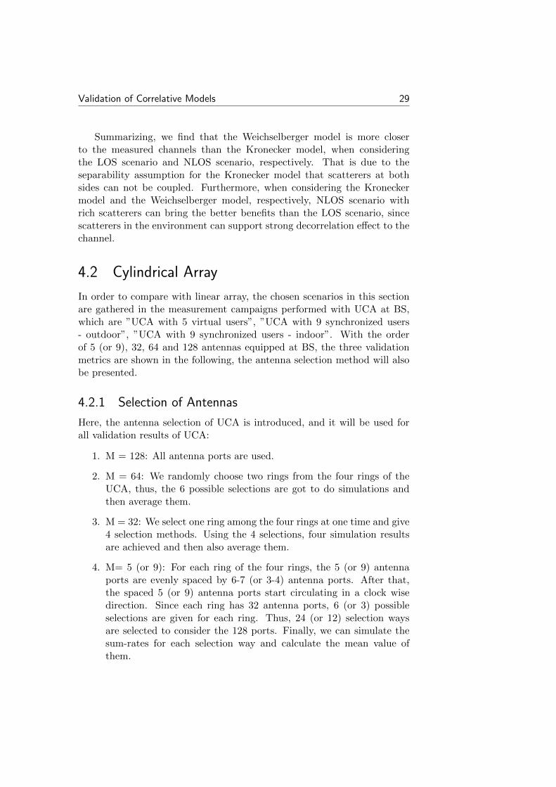
In order to compare with linear array, the chosen scenarios in this sectionare gathered in the measurement campaigns performed with UCA at BS,which are ”UCA with 5 virtual users”, ”UCA with 9 synchronized users- outdoor”, ”UCA with 9 synchronized users - indoor”. With the orderof 5 (or 9), 32, 64 and 128 antennas equipped at BS, the three validationmetrics are shown in the following, the antenna selection method will alsobe presented.
4.2.1 Selection of Antennas
Here, the antenna selection of UCA is introduced, and it will be used forall validation results of UCA:
1. M = 128: All antenna ports are used.
2. M = 64: We randomly choose two rings from the four rings of theUCA, thus, the 6 possible selections are got to do simulations andthen average them.
3. M = 32: We select one ring among the four rings at one time and give4 selection methods. Using the 4 selections, four simulation resultsare achieved and then also average them.
4. M= 5 (or 9): For each ring of the four rings, the 5 (or 9) antennaports are evenly spaced by 6-7 (or 3-4) antenna ports. After that,the spaced 5 (or 9) antenna ports start circulating in a clock wisedirection. Since each ring has 32 antenna ports, 6 (or 3) possibleselections are given for each ring. Thus, 24 (or 12) selection waysare selected to consider the 128 ports. Finally, we can simulate thesum-rates for each selection way and calculate the mean value ofthem.
30 Validation of Correlative Models
4.2.2 UCA with 5 Virtual Users
In this subsection, the measured data is from the second measurementcampaign. It is important to know that the measured data is from thefirst half of the 40 positions, since the user travels long distance over thepositions and the environment has changed. As mentioned in the section4.1, validation results of the two correlative model are based on the samescenario as before in order to compare the performance of the UCA andULA.
LOS Scenario
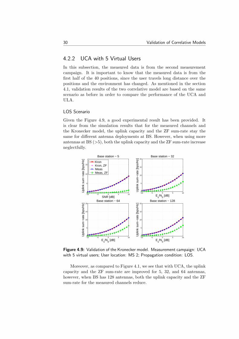
Given the Figure 4.9, a good experimental result has been provided. Itis clear from the simulation results that for the measured channels andthe Kronecker model, the uplink capacity and the ZF sum-rate stay thesame for different antenna deployments at BS. However, when using moreantennas at BS (>5), both the uplink capacity and the ZF sum-rate increaseneglectfully.
−10 −5 0 5 100
5
10
15
SNR [dB]
Upl
ink
sum
−ra
te [b
ps/H
z]
Base station − 5
KronKron, ZFMeasMeas, ZF
−10 −5 0 5 100
5
10
15
20
Es/N
0 [dB]
Upl
ink
sum
−ra
te [b
ps/H
z]
Base station − 32
−10 −5 0 5 100
5
10
15
20
Es/N
0 [dB]
Upl
ink
sum
−ra
te [b
ps/H
z]
Base station − 64
−10 −5 0 5 100
5
10
15
20
Es/N
0 [dB]
Upl
ink
sum
−ra
te [b
ps/H
z]
Base station − 128
Figure 4.9: Validation of the Kronecker model. Measurement campaign: UCAwith 5 virtual users; User location: MS 2; Propagation condition: LOS.
Moreover, as compared to Figure 4.1, we see that with UCA, the uplinkcapacity and the ZF sum-rate are improved for 5, 32, and 64 antennas,however, when BS has 128 antennas, both the uplink capacity and the ZFsum-rate for the measured channels reduce.
Validation of Correlative Models 31
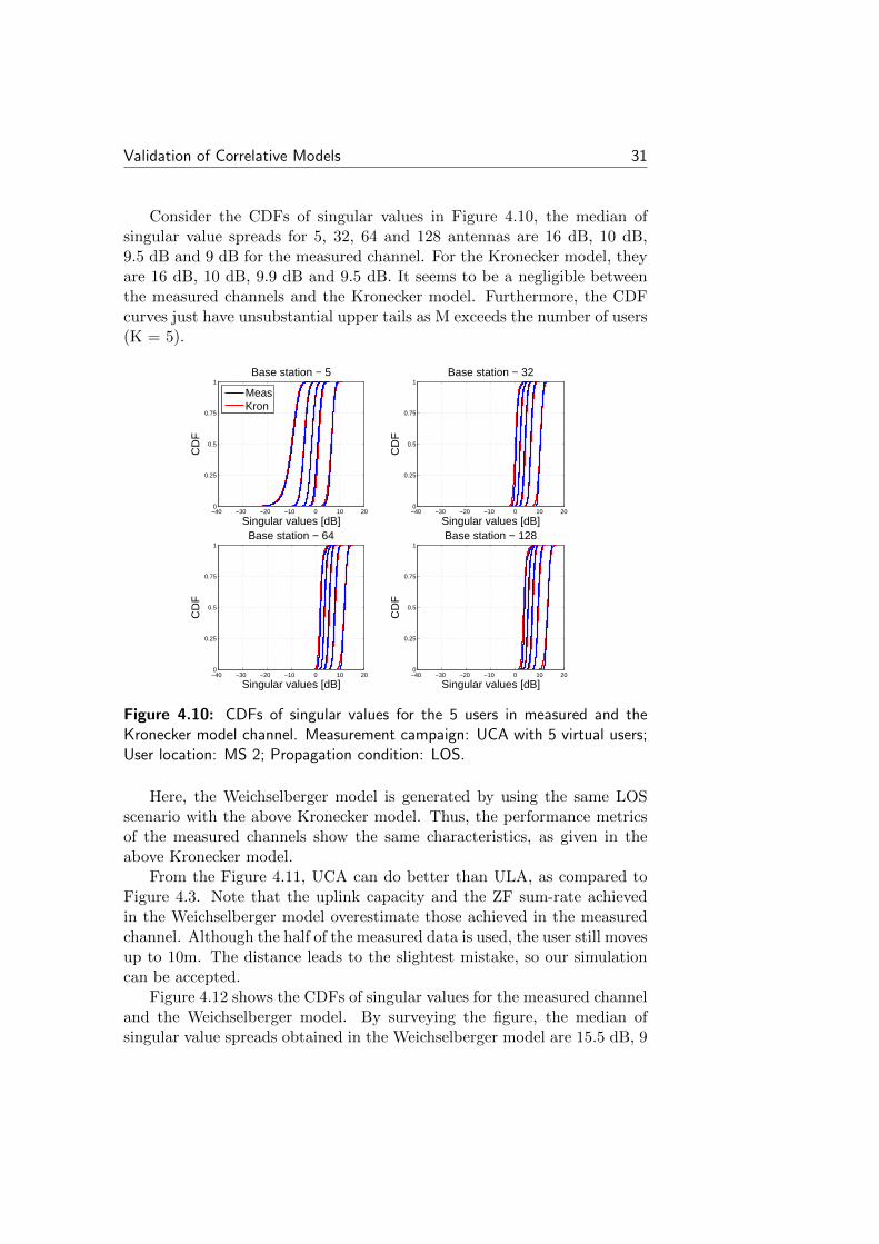
Consider the CDFs of singular values in Figure 4.10, the median ofsingular value spreads for 5, 32, 64 and 128 antennas are 16 dB, 10 dB,9.5 dB and 9 dB for the measured channel. For the Kronecker model, theyare 16 dB, 10 dB, 9.9 dB and 9.5 dB. It seems to be a negligible betweenthe measured channels and the Kronecker model. Furthermore, the CDFcurves just have unsubstantial upper tails as M exceeds the number of users(K = 5).
−40 −30 −20 −10 0 10 200
0.25
0.5
0.75
1
Singular values [dB]
CD
F
Base station − 5
MeasKron
−40 −30 −20 −10 0 10 200
0.25
0.5
0.75
1
Singular values [dB]
CD
F
Base station − 32
−40 −30 −20 −10 0 10 200
0.25
0.5
0.75
1
Singular values [dB]
CD
F
Base station − 64
−40 −30 −20 −10 0 10 200
0.25
0.5
0.75
1
Singular values [dB]
CD
F
Base station − 128
Figure 4.10: CDFs of singular values for the 5 users in measured and theKronecker model channel. Measurement campaign: UCA with 5 virtual users;User location: MS 2; Propagation condition: LOS.
Here, the Weichselberger model is generated by using the same LOSscenario with the above Kronecker model. Thus, the performance metricsof the measured channels show the same characteristics, as given in theabove Kronecker model.
From the Figure 4.11, UCA can do better than ULA, as compared toFigure 4.3. Note that the uplink capacity and the ZF sum-rate achievedin the Weichselberger model overestimate those achieved in the measuredchannel. Although the half of the measured data is used, the user still movesup to 10m. The distance leads to the slightest mistake, so our simulationcan be accepted.
Figure 4.12 shows the CDFs of singular values for the measured channeland the Weichselberger model. By surveying the figure, the median ofsingular value spreads obtained in the Weichselberger model are 15.5 dB, 9

32 Validation of Correlative Models
−10 −5 0 5 100
5
10
15
20
Es/N
0 [dB]
Upl
ink
sum
−ra
te [b
ps/H
z]
Base station − 5
WeichWeich, ZFMeasMeas, ZF
−10 −5 0 5 100
5
10
15
20
Es/N
0 [dB]
Upl
ink
sum
−ra
te [b
ps/H
z]
Base station − 32
−10 −5 0 5 100
5
10
15
20
Es/N
0 [dB]
Upl
ink
sum
−ra
te [b
ps/H
z]
Base station − 64
−10 −5 0 5 100
5
10
15
20
Es/N
0 [dB]
Upl
ink
sum
−ra
te [b
ps/H
z]
Base station − 128
Figure 4.11: Validation of the Weichselberger model. Measurement cam-paign: UCA with 5 virtual users; User location: MS 2; Propagation condition:LOS.
−40 −30 −20 −10 0 10 200
0.25
0.5
0.75
1
Singular values [dB]
CD
F
Base station − 5
MeasWeich
−40 −30 −20 −10 0 10 200
0.25
0.5
0.75
1
Singular values [dB]
CD
F
Base station − 32
−40 −30 −20 −10 0 10 200
0.25
0.5
0.75
1
Singular values [dB]
CD
F
Base station − 64
−40 −30 −20 −10 0 10 200
0.25
0.5
0.75
1
Singular values [dB]
CD
F
Base station − 128
Figure 4.12: CDFs of singular values for the 5 users in measured and theWeichselberger model channel. Measurement campaign: UCA with 5 virtualusers; User location: MS 2; Propagation condition: LOS.
Validation of Correlative Models 33
dB, 9 dB and 8.9 dB for different antenna deployment. When M is largerthan 5, CDF curves become more stable.
In this LOS scenario, the contribution of the correlative models to themeasured channels from massive MIMO can be viewed as sameness. TheWeichselberger model has been shown to be accurate than the Kroneckermodel in the literature, however, it does not be supported, when consideringmassive MIMO performed with UCA at BS.
NLOS Scenario
In contrast to the LOS scenario above, validation results of correlativemodels for the NLOS scenario will be given in the next paragraphs.
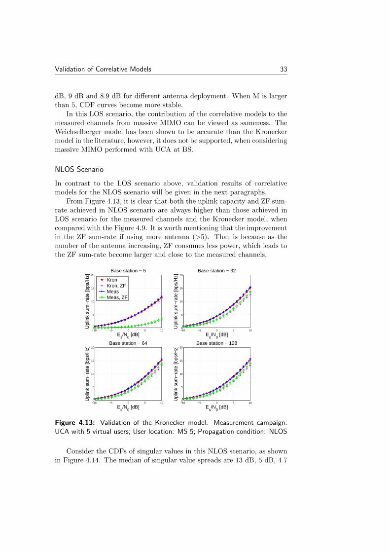
From Figure 4.13, it is clear that both the uplink capacity and ZF sum-rate achieved in NLOS scenario are always higher than those achieved inLOS scenario for the measured channels and the Kronecker model, whencompared with the Figure 4.9. It is worth mentioning that the improvementin the ZF sum-rate if using more antenna (>5). That is because as thenumber of the antenna increasing, ZF consumes less power, which leads tothe ZF sum-rate become larger and close to the measured channels.
−10 −5 0 5 100
5
10
15
20
Es/N
0 [dB]
Upl
ink
sum
−ra
te [b
ps/H
z]
Base station − 5
KronKron, ZFMeasMeas, ZF
−10 −5 0 5 100
5
10
15
20
Es/N
0 [dB]
Upl
ink
sum
−ra
te [b
ps/H
z]
Base station − 32
−10 −5 0 5 100
5
10
15
20
Es/N
0 [dB]
Upl
ink
sum
−ra
te [b
ps/H
z]
Base station − 64
−10 −5 0 5 100
5
10
15
20
Es/N
0 [dB]
Upl
ink
sum
−ra
te [b
ps/H
z]
Base station − 128
Figure 4.13: Validation of the Kronecker model. Measurement campaign:UCA with 5 virtual users; User location: MS 5; Propagation condition: NLOS
Consider the CDFs of singular values in this NLOS scenario, as shownin Figure 4.14. The median of singular value spreads are 13 dB, 5 dB, 4.7

34 Validation of Correlative Models
dB and 4.5 dB for the measured channels when equipping 5, 32, 64 and 128antennas at BS. Furthermore, the median values for the Kronecker model(13 dB, 5.5 dB, 5 dB and 5 dB) also can be caught for different antennanumber in the figure. The median values in this scenario for both themeasured channels and the Kronecker model are smaller than the medianvalues achieved in the LOS conditions (see Figure 4.10). Moreover, it canbe observed that the lines become tighter as the antenna increases, that letsingular value spreads become much more stable.
−40 −30 −20 −10 0 10 200
0.25
0.5
0.75
1
Singular values [dB]
CD
F
Base station − 5
MeasKron
−40 −30 −20 −10 0 10 200
0.25
0.5
0.75
1
Singular values [dB]
CD
F
Base station − 32
−40 −30 −20 −10 0 10 200
0.25
0.5
0.75
1
Singular values [dB]
CD
F
Base station − 64
−40 −30 −20 −10 0 10 200
0.25
0.5
0.75
1
Singular values [dB]
CD
F
Base station − 128
Figure 4.14: CDFs of singular values for the 5 users in measured and theKronecker model channel. Measurement campaign: UCA with 5 virtual users;User location: MS 5; Propagation condition: NLOS.
Using the measured data from the NLOS scenario, the Weichselbergermodel is generated. After that, the metrics are computed. ObservingFigure 4.15 and Figure 4.13, it is difficult to distinguish both figures. Thatcan prove that we can not determine which model is more accurate.
As can be seen in Figure 4.16, singular values for the Weichselber modelgive the same characteristic as the Kronecker model, when compared tothose in Figure 4.14.
When considering the NLOS scenario, validation metrics created by theKronecker model give the same variation as shown in the Weichselbergermodel. Thus, the Weichselberger model is not more accurate than theKronecker model.
Clearly, compared to the section 4.1, UCA shows good performance
Validation of Correlative Models 35
−10 −5 0 5 100
5
10
15
20
Es/N
0 [dB]
Upl
ink
sum
−ra
te [b
ps/H
z]
Base station − 5
WeichWeich, ZFMeasMeas, ZF
−10 −5 0 5 100
5
10
15
20
Es/N
0 [dB]
Upl
ink
sum
−ra
te [b
ps/H
z]
Base station − 32
−10 −5 0 5 100
5
10
15
20
Es/N
0 [dB]
Upl
ink
sum
−ra
te [b
ps/H
z]
Base station − 64
−10 −5 0 5 100
5
10
15
20
Es/N
0 [dB]
Upl
ink
sum
−ra
te [b
ps/H
z]Base station − 128
Figure 4.15: Validation of the Weichselberger model. Measurement cam-paign: UCA with 5 virtual users; User location: MS 5; Propagation condition:NLOS
−40 −30 −20 −10 0 10 200
0.25
0.5
0.75
1
Singular values [dB]
CD
F
Base station − 5
MeasWeich
−40 −30 −20 −10 0 10 200
0.25
0.5
0.75
1
Singular values [dB]
CD
F
Base station − 32
−40 −30 −20 −10 0 10 200
0.25
0.5
0.75
1
Singular values [dB]
CD
F
Base station − 64
−40 −30 −20 −10 0 10 200
0.25
0.5
0.75
1
Singular values [dB]
CD
F
Base station − 128
Figure 4.16: CDFs of singular values for the 5 users in measured and theWeichselberger model channel. Measurement campaign: UCA with 5 virtualusers; User location: MS 5; Propagation condition: NLOS.
36 Validation of Correlative Models
than ULA. On the other hand, it is very likely that the two correlativemodels are great models to model the measured channel by the validationmetrics, when considering the measured data from the second measurementcampaign. And in the future, it is really needed to do more research forthe two correlative models.
However, for this measurement campaign, we measured the 40 positionswith a inter-spacing of 0.5m, that results in the variation of the environ-ment. To reduce the changes of the environment, we remove the last halfof the measured data for our simulation, however, that still leads to somechallenges.
4.2.3 UCA with 9 Synchronized Users - Outdoor
It is important the fact that the third measurement campaign employs9 simultaneous real users to communicate with the UCA BS. Thus, it isobvious that the correlative models modelled in this measurement campaigncould have significant differences relative to the measurement campaignemployed 5 virtual users.
As simulated in the first two measurement campaigns, the LOS scenarioand the NLOS scenario were considered. We study the same two kinds ofscenarios for this campaign, and except for the LOS condition and theNLOS condition, we also consider a heavy crowed condition with 10-12persons. The measurement sites used in this subsection has been shown inFigure 2.3a.
The investigated scenarios are:
• The first used scenario is measured at MS 1, as shown in Figure 2.3a,and MS 1 has LOS condition. Furthermore, the 9 active users arecrowded by another 10 to 12 persons or not.
• The another scenario is performed at MS 3, that has NLOS condition.The 9 active users with the crowd and without the crowd also beobserved.
LOS Scenarios
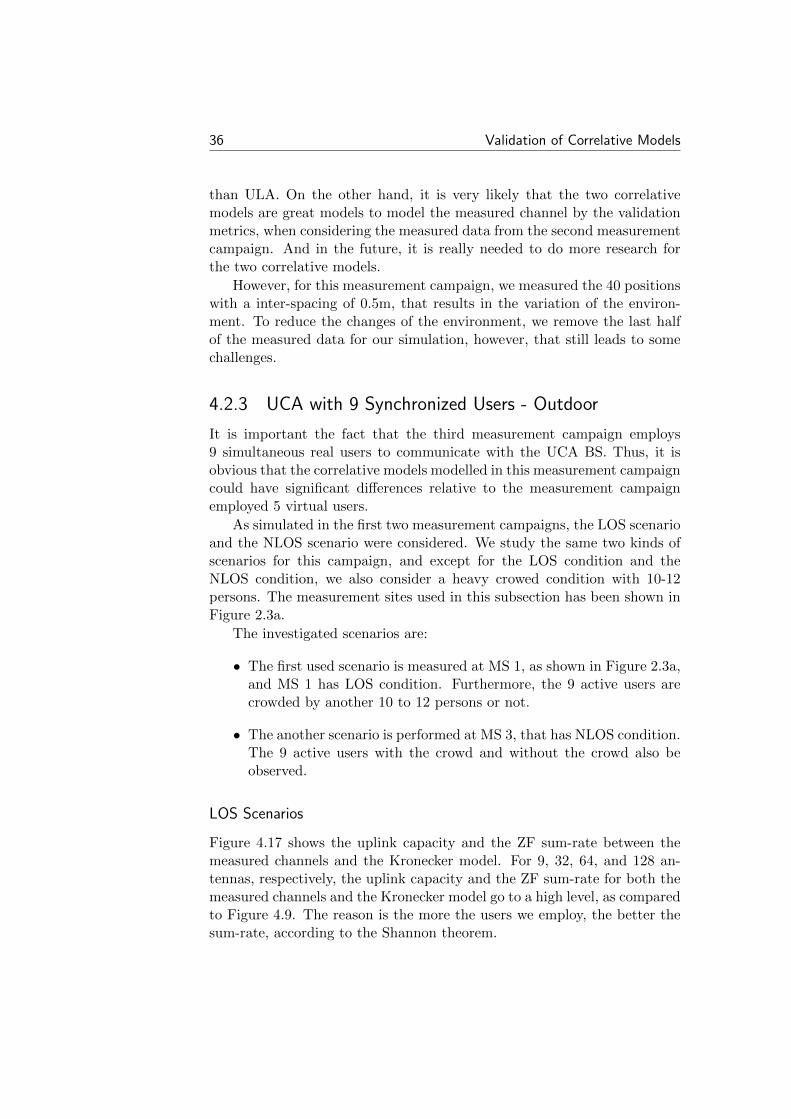
Figure 4.17 shows the uplink capacity and the ZF sum-rate between themeasured channels and the Kronecker model. For 9, 32, 64, and 128 an-tennas, respectively, the uplink capacity and the ZF sum-rate for both themeasured channels and the Kronecker model go to a high level, as comparedto Figure 4.9. The reason is the more the users we employ, the better thesum-rate, according to the Shannon theorem.
Validation of Correlative Models 37
−10 −5 0 5 100
5
10
15
20
25
30
Es/N
0 [dB]
Upl
ink
sum
−ra
te [b
ps/H
z]
Base station − 9
KronKron, ZFMeasMeas, ZF
−10 −5 0 5 100
5
10
15
20
25
30
Es/N
0 [dB]
Upl
ink
sum
−ra
te [b
ps/H
z]
Base station − 32
−10 −5 0 5 100
5
10
15
20
25
30
Es/N
0 [dB]
Upl
ink
sum
−ra
te [b
ps/H
z]
Base station − 64
−10 −5 0 5 100
5
10
15
20
25
30
Es/N
0 [dB]
Upl
ink
sum
−ra
te [b
ps/H
z]Base station − 128
Figure 4.17: Validation of the Kronecker model. Measurement campaign:UCA with 9 synchronized users - outdoor; User location: MS 1; Propagationcondition: LOS - Crowd.
−30 −20 −10 0 10 200
0.25
0.5
0.75
1
Singular values [dB]
CD
F
Base station − 9
MeasKron
−30 −20 −10 0 10 200
0.25
0.5
0.75
1
Singular values [dB]
CD
F
Base station − 32
−30 −20 −10 0 10 200
0.25
0.5
0.75
1
Singular values [dB]
CD
F
Base station − 64
−30 −20 −10 0 10 200
0.25
0.5
0.75
1
Singular values [dB]
CD
F
Base station − 128
Figure 4.18: CDFs of singular values for the 9 users in measured and theKronecker model channel. Measurement campaign: UCA with 9 synchronizedusers - outdoor; User location: MS 1; Propagation condition: LOS - Crowd.
38 Validation of Correlative Models
To the best of our knowledge, the Kronecker model consistently under-estimates the sum-rates of the channels, however, in this scenario, it hasbeen shown to be accurate for characterizing real-life channels. Thus, itis reasonable to state that the Kronecker model does a good job of sim-ulating the measured channel. As a matter of fact, since the number ofthe scatterers limits the achievable sum-rates, the uplink capacity and theZF sum-rate for both the measure channels and the kronecker model donot increase that significantly as the number of the antenna at BS, whenhaving more antennas (>9).
−10 −5 0 5 100
5
10
15
20
25
30
Es/N
0 [dB]
Upl
ink
sum
−ra
te [b
ps/H
z]
Base station − 9
WeichWeich, ZFMeasMeas, ZF
−10 −5 0 5 100
5
10
15
20
25
30
Es/N
0 [dB]
Upl
ink
sum
−ra
te [b
ps/H
z]
Base station − 32
−10 −5 0 5 100
5
10
15
20
25
30
Es/N
0 [dB]
Upl
ink
sum
−ra
te [b
ps/H
z]
Base station − 64
−10 −5 0 5 100
5
10
15
20
25
30
Es/N
0 [dB]
Upl
ink
sum
−ra
te [b
ps/H
z]
Base station − 128
Figure 4.19: Validation of the Weichselberger model. Measurement cam-paign: UCA with 9 synchronized users - outdoor; User location: MS 1; Prop-agation condition: LOS - Crowd.
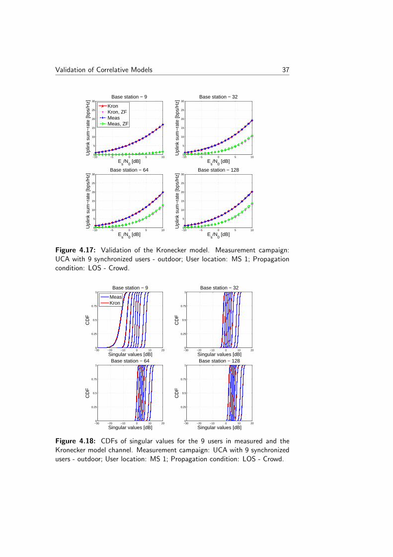
Figure 4.18 reveals that the median of singular value spreads are 19dB, 12 dB, 11 dB and 10 dB for all the cases of 9, 32, 64 and 128 BSantennas for the measured channels, and 19.5 dB, 12 dB, 11 dB and 10dB for the Kronecker model. Results show that the median values becomesmaller as increasing the number of antennas at BS. That means that userchannel decorrelate if we increase the number of the antennas at BS, thatcan decrease the correlation between the channels and leads to a muchbetter channel orthogonality in the measured channels and the Kroneckermodel.
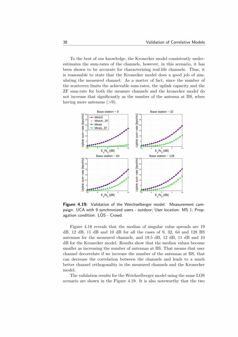
The validation results for the Weichselberger model using the same LOSscenario are shown in the Figure 4.19. It is also noteworthy that the two

Validation of Correlative Models 39
correlative models show the same performance, by seeing Figure 4.17 andFigure 4.19.
As discussed in the [15], the Kronecker model performs poorly for thelarger number of antenna when using real-life data. However, the perfor-mance metrics for this scenario imply that the Kronecker model can handlethe measured data obtained from a large number of antennas system. And,we, here, demonstrate once again the Weichselberger model is not moreaccurate than the Kronecker model.
For Weichselberger model, the median of singular value spreads are 19dB, 11.5 dB, 10 dB and 10 dB when BS uses 9, 32, 64 and 128 antennaelements (see Figure 4.20). In such a case, it give the same performance asshown in Figure 4.18.
−30 −20 −10 0 10 200
0.25
0.5
0.75
1
Singular values [dB]
CD
F
Base station − 9
MeasWeich
−30 −20 −10 0 10 200
0.25
0.5
0.75
1
Singular values [dB]
CD
F
Base station − 32
−30 −20 −10 0 10 200
0.25
0.5
0.75
1
Singular values [dB]
CD
F
Base station − 64
−30 −20 −10 0 10 200
0.25
0.5
0.75
1
Singular values [dB]
CD
F
Base station − 128
Figure 4.20: CDFs of singular values for the 9 users in measured and theWeichselberger model channel. Measurement campaign: UCA with 9 synchro-nized users - outdoor; User location: MS 1; Propagation condition: LOS -Crowd.
Let us next consider the case where there are no crowd in the locationMS 1. In such a case, it can be more possible to point out the contributionof the crowd.
The uplink capacity and the ZF sum-rate for both the measured chan-nels and the Kronecker model have been shown in Figure 4.21. The figurepresents the same characteristics as Figure 4.17, and we can not look atthe difference between them.
40 Validation of Correlative Models
−10 −5 0 5 100
5
10
15
20
25
30
Es/N
0 [dB]
Upl
ink
sum
−ra
te [b
ps/H
z]
Base station − 9
KronKron, ZFMeasMeas, ZF
−10 −5 0 5 100
5
10
15
20
25
30
Es/N
0 [dB]
Upl
ink
sum
−ra
te [b
ps/H
z]
Base station − 32
−10 −5 0 5 100
5
10
15
20
25
30
Es/N
0 [dB]
Upl
ink
sum
−ra
te [b
ps/H
z]
Base station − 64
−10 −5 0 5 100
5
10
15
20
25
30
Es/N
0 [dB]
Upl
ink
sum
−ra
te [b
ps/H
z]
Base station − 128
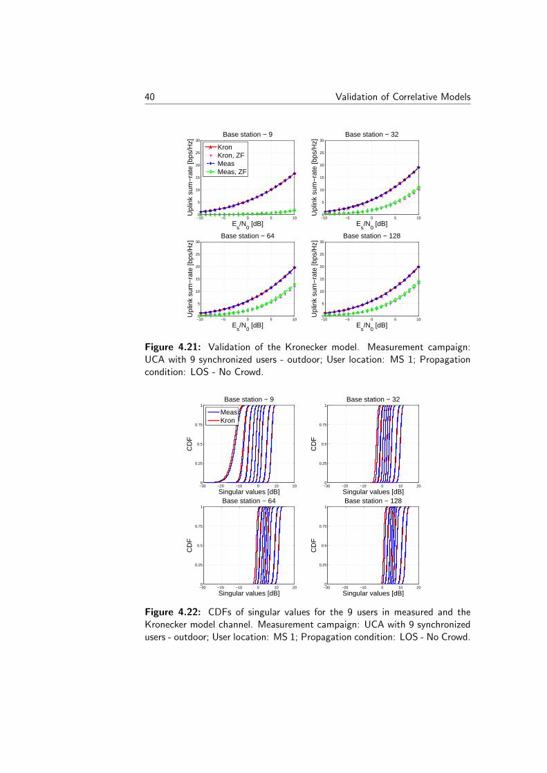
Figure 4.21: Validation of the Kronecker model. Measurement campaign:UCA with 9 synchronized users - outdoor; User location: MS 1; Propagationcondition: LOS - No Crowd.
−30 −20 −10 0 10 200
0.25
0.5
0.75
1
Singular values [dB]
CD
F
Base station − 9
MeasKron
−30 −20 −10 0 10 200
0.25
0.5
0.75
1
Singular values [dB]
CD
F
Base station − 32
−30 −20 −10 0 10 200
0.25
0.5
0.75
1
Singular values [dB]
CD
F
Base station − 64
−30 −20 −10 0 10 200
0.25
0.5
0.75
1
Singular values [dB]
CD
F
Base station − 128
Figure 4.22: CDFs of singular values for the 9 users in measured and theKronecker model channel. Measurement campaign: UCA with 9 synchronizedusers - outdoor; User location: MS 1; Propagation condition: LOS - No Crowd.
Validation of Correlative Models 41
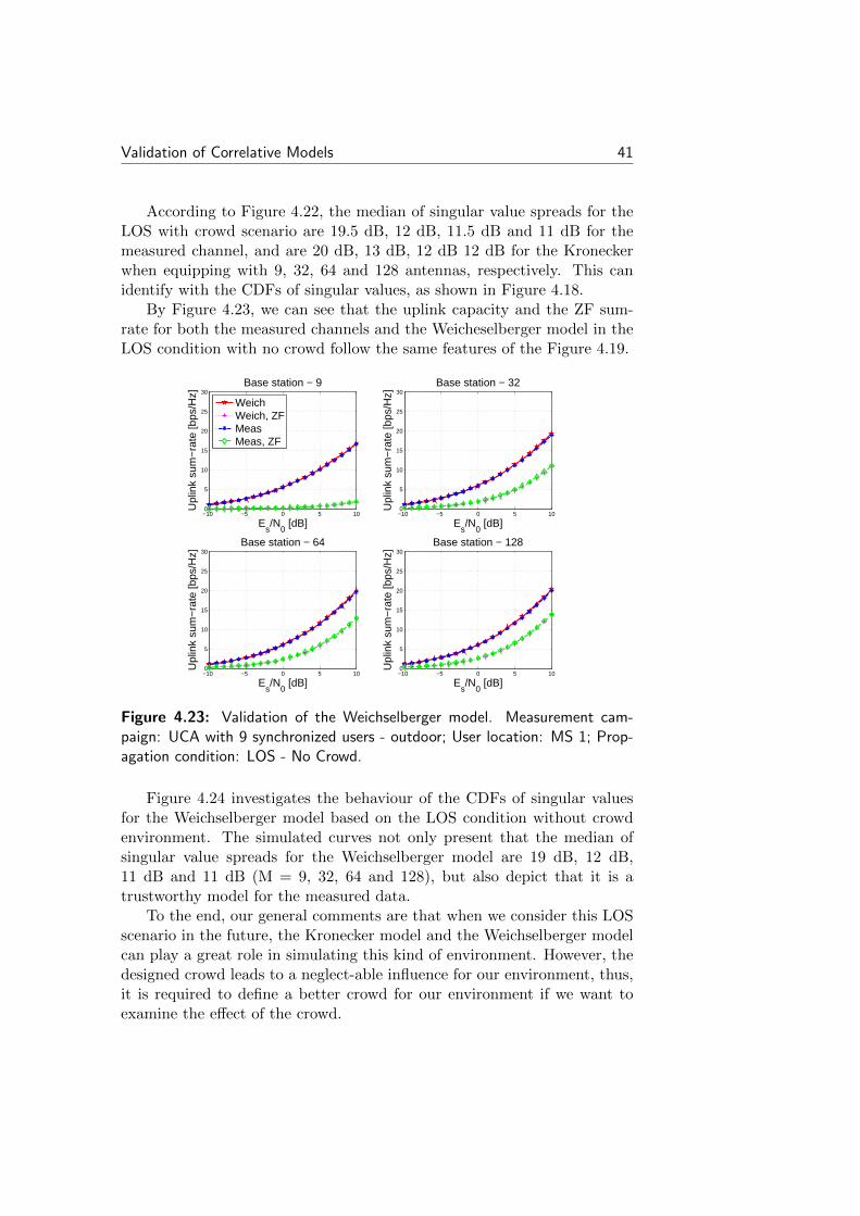
According to Figure 4.22, the median of singular value spreads for theLOS with crowd scenario are 19.5 dB, 12 dB, 11.5 dB and 11 dB for themeasured channel, and are 20 dB, 13 dB, 12 dB 12 dB for the Kroneckerwhen equipping with 9, 32, 64 and 128 antennas, respectively. This canidentify with the CDFs of singular values, as shown in Figure 4.18.
By Figure 4.23, we can see that the uplink capacity and the ZF sum-rate for both the measured channels and the Weicheselberger model in theLOS condition with no crowd follow the same features of the Figure 4.19.
−10 −5 0 5 100
5
10
15
20
25
30
Es/N
0 [dB]
Upl
ink
sum
−ra
te [b
ps/H
z]
Base station − 9
WeichWeich, ZFMeasMeas, ZF
−10 −5 0 5 100
5
10
15
20
25
30
Es/N
0 [dB]
Upl
ink
sum
−ra
te [b
ps/H
z]Base station − 32
−10 −5 0 5 100
5
10
15
20
25
30
Es/N
0 [dB]
Upl
ink
sum
−ra
te [b
ps/H
z]
Base station − 64
−10 −5 0 5 100
5
10
15
20
25
30
Es/N
0 [dB]
Upl
ink
sum
−ra
te [b
ps/H
z]
Base station − 128
Figure 4.23: Validation of the Weichselberger model. Measurement cam-paign: UCA with 9 synchronized users - outdoor; User location: MS 1; Prop-agation condition: LOS - No Crowd.
Figure 4.24 investigates the behaviour of the CDFs of singular valuesfor the Weichselberger model based on the LOS condition without crowdenvironment. The simulated curves not only present that the median ofsingular value spreads for the Weichselberger model are 19 dB, 12 dB,11 dB and 11 dB (M = 9, 32, 64 and 128), but also depict that it is atrustworthy model for the measured data.
To the end, our general comments are that when we consider this LOSscenario in the future, the Kronecker model and the Weichselberger modelcan play a great role in simulating this kind of environment. However, thedesigned crowd leads to a neglect-able influence for our environment, thus,it is required to define a better crowd for our environment if we want toexamine the effect of the crowd.
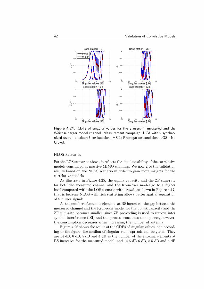
42 Validation of Correlative Models
−30 −20 −10 0 10 200
0.25
0.5
0.75
1
Singular values [dB]
CD
F
Base station − 9
MeasWeich
−30 −20 −10 0 10 200
0.25
0.5
0.75
1
Singular values [dB]
CD
F
Base station − 32
−30 −20 −10 0 10 200
0.25
0.5
0.75
1
Singular values [dB]
CD
F
Base station − 64
−30 −20 −10 0 10 200
0.25
0.5
0.75
1
Singular values [dB]
CD
F
Base station − 128
Figure 4.24: CDFs of singular values for the 9 users in measured and theWeichselberger model channel. Measurement campaign: UCA with 9 synchro-nized users - outdoor; User location: MS 1; Propagation condition: LOS - NoCrowd.
NLOS Scenarios
For the LOS scenarios above, it reflects the simulate ability of the correlativemodels considered at massive MIMO channels. We now give the validationresults based on the NLOS scenario in order to gain more insights for thecorrelative models.
As illustrate in Figure 4.25, the uplink capacity and the ZF sum-ratefor both the measured channel and the Kronecker model go to a higherlevel compared with the LOS scenario with crowd, as shown in Figure 4.17,that is because NLOS with rich scattering allows better spatial separationof the user signals.
As the number of antenna elements at BS increases, the gap between themeasured channel and the Kronecker model for the uplink capacity and theZF sum-rate becomes smaller, since ZF pre-coding is used to remove intersymbol interference (ISI) and this process consumes some power, however,the consumption decreases when increasing the number of antenna.
Figure 4.26 shows the result of the CDFs of singular values, and accord-ing to the figure, the median of singular value spreads can be given. Theyare 14 dB, 6 dB, 5 dB and 4 dB as the number of the antenna elements atBS increases for the measured model, and 14.5 dB 6 dB, 5.5 dB and 5 dB
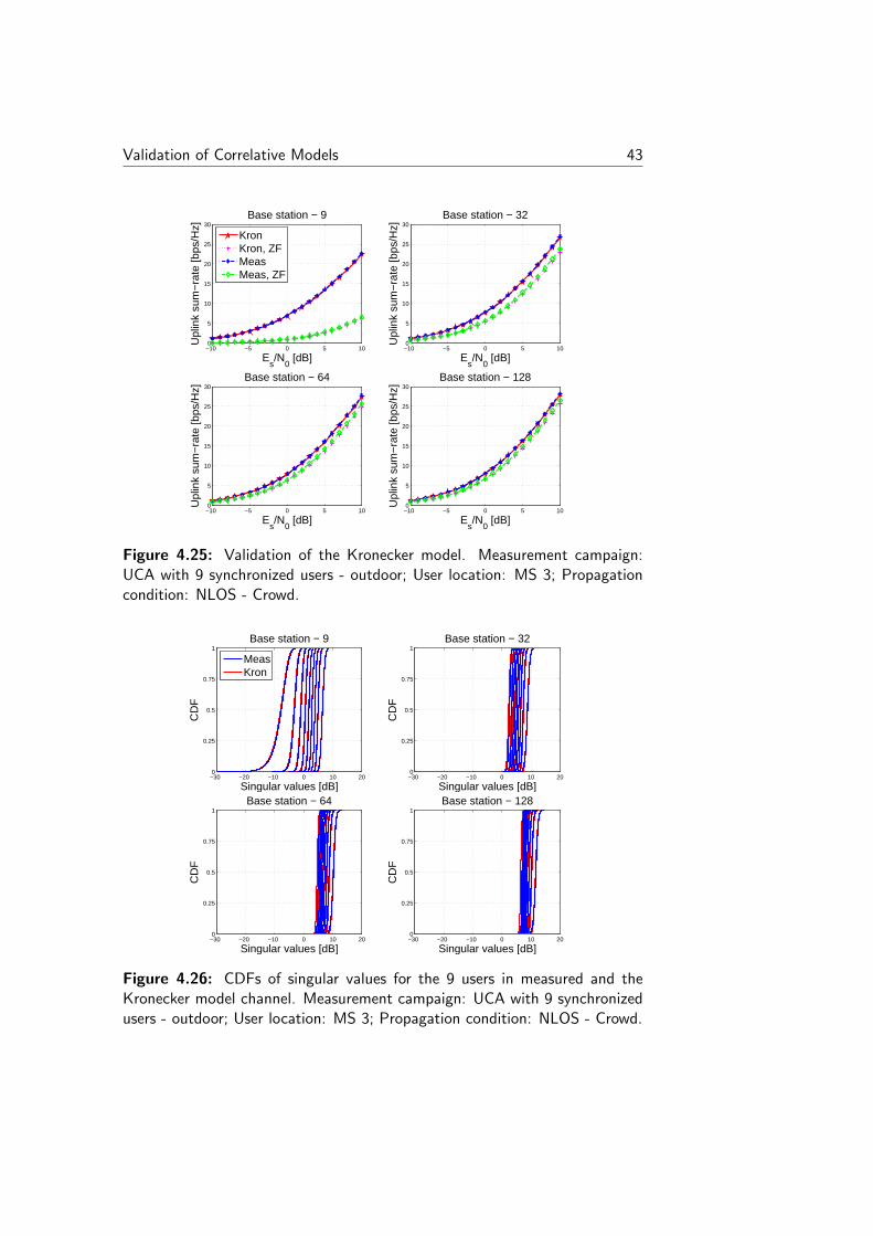
Validation of Correlative Models 43
−10 −5 0 5 100
5
10
15
20
25
30
Es/N
0 [dB]
Upl
ink
sum
−ra
te [b
ps/H
z]
Base station − 9
KronKron, ZFMeasMeas, ZF
−10 −5 0 5 100
5
10
15
20
25
30
Es/N
0 [dB]
Upl
ink
sum
−ra
te [b
ps/H
z]
Base station − 32
−10 −5 0 5 100
5
10
15
20
25
30
Es/N
0 [dB]
Upl
ink
sum
−ra
te [b
ps/H
z]
Base station − 64
−10 −5 0 5 100
5
10
15
20
25
30
Es/N
0 [dB]
Upl
ink
sum
−ra
te [b
ps/H
z]Base station − 128
Figure 4.25: Validation of the Kronecker model. Measurement campaign:UCA with 9 synchronized users - outdoor; User location: MS 3; Propagationcondition: NLOS - Crowd.
−30 −20 −10 0 10 200
0.25
0.5
0.75
1
Singular values [dB]
CD
F
Base station − 9
MeasKron
−30 −20 −10 0 10 200
0.25
0.5
0.75
1
Singular values [dB]
CD
F
Base station − 32
−30 −20 −10 0 10 200
0.25
0.5
0.75
1
Singular values [dB]
CD
F
Base station − 64
−30 −20 −10 0 10 200
0.25
0.5
0.75
1
Singular values [dB]
CD
F
Base station − 128
Figure 4.26: CDFs of singular values for the 9 users in measured and theKronecker model channel. Measurement campaign: UCA with 9 synchronizedusers - outdoor; User location: MS 3; Propagation condition: NLOS - Crowd.

44 Validation of Correlative Models
−10 −5 0 5 100
5
10
15
20
25
30
Es/N
0 [dB]
Upl
ink
sum
−ra
te [b
ps/H
z]
Base station − 9
WeichWeich, ZFMeasMeas, ZF
−10 −5 0 5 100
5
10
15
20
25
30
Es/N
0 [dB]
Upl
ink
sum
−ra
te [b
ps/H
z]
Base station − 32
−10 −5 0 5 100
5
10
15
20
25
30
Es/N
0 [dB]
Upl
ink
sum
−ra
te [b
ps/H
z]
Base station − 64
−10 −5 0 5 100
5
10
15
20
25
30
Es/N
0 [dB]
Upl
ink
sum
−ra
te [b
ps/H
z]
Base station − 128
Figure 4.27: Validation of the Weichselberger model. Measurement cam-paign: UCA with 9 synchronized users - outdoor; User location: MS 3; Prop-agation condition: NLOS - Crowd.
for the Kronecker model.
It should be noted that the median values become significantly smallerin NLOS condition, as compared to those in the corresponding LOS con-dition. Moreover, the singular value spreads have lesser variations for themeasured channel and the Kronecker model if M = 9, after that, the sin-gular value spreads can be treated as a constant for M = 32, 64 and 128.This model provides performance very close to the measured channel andgives better spatial separation of the user signals.
It is assumed that the Weichselberger model is confirmed. By usingthat, the uplink capacity and the ZF sum-rate can be achieved, as illus-trated in 4.27. By taking into account the figure, it is hard to be furtherdistinguished for the measured channels and the Weichselberger model andit is also difficulty to specify the difference between this figure and the Fig-ure 4.25. Accordingly, the two described correlative models is supposed tohave ability to model the measured channel when we choose this scenario.
In Figure 4.28, the median of singular value spreads (14 dB, 6 dB 5dB and 4.5 dB) for the Weichselberger model can be achieved accordingto equipping 9, 32, 64 and 128 antenna elements at BS. This figure can beexplained as the Figure 4.26, as they match each other very well.
As can be seen in Figure 4.29 and Figure 4.25, both figures are the
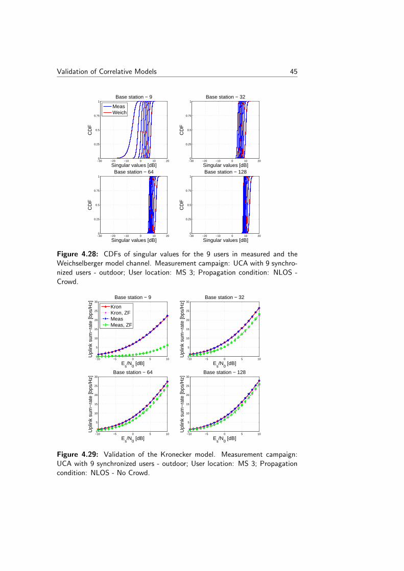
Validation of Correlative Models 45
−30 −20 −10 0 10 200
0.25
0.5
0.75
1
Singular values [dB]
CD
F
Base station − 9
MeasWeich
−30 −20 −10 0 10 200
0.25
0.5
0.75
1
Singular values [dB]
CD
F
Base station − 32
−30 −20 −10 0 10 200
0.25
0.5
0.75
1
Singular values [dB]
CD
F
Base station − 64
−30 −20 −10 0 10 200
0.25
0.5
0.75
1
Singular values [dB]
CD
F
Base station − 128
Figure 4.28: CDFs of singular values for the 9 users in measured and theWeichselberger model channel. Measurement campaign: UCA with 9 synchro-nized users - outdoor; User location: MS 3; Propagation condition: NLOS -Crowd.
−10 −5 0 5 100
5
10
15
20
25
30
Es/N
0 [dB]
Upl
ink
sum
−ra
te [b
ps/H
z]
Base station − 9
KronKron, ZFMeasMeas, ZF
−10 −5 0 5 100
5
10
15
20
25
30
Es/N
0 [dB]
Upl
ink
sum
−ra
te [b
ps/H
z]
Base station − 32
−10 −5 0 5 100
5
10
15
20
25
30
Es/N
0 [dB]
Upl
ink
sum
−ra
te [b
ps/H
z]
Base station − 64
−10 −5 0 5 100
5
10
15
20
25
30
Es/N
0 [dB]
Upl
ink
sum
−ra
te [b
ps/H
z]
Base station − 128
Figure 4.29: Validation of the Kronecker model. Measurement campaign:UCA with 9 synchronized users - outdoor; User location: MS 3; Propagationcondition: NLOS - No Crowd.
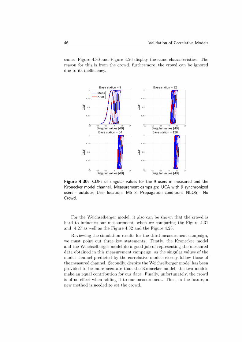
46 Validation of Correlative Models
same. Figure 4.30 and Figure 4.26 display the same characteristics. Thereason for this is from the crowd, furthermore, the crowd can be ignoreddue to its inefficiency.
−30 −20 −10 0 10 200
0.25
0.5
0.75
1
Singular values [dB]
CD
FBase station − 9
MeasKron
−30 −20 −10 0 10 200
0.25
0.5
0.75
1
Singular values [dB]
CD
F
Base station − 32
−30 −20 −10 0 10 200
0.25
0.5
0.75
1
Singular values [dB]
CD
F
Base station − 64
−30 −20 −10 0 10 200
0.25
0.5
0.75
1
Singular values [dB]
CD
F
Base station − 128
Figure 4.30: CDFs of singular values for the 9 users in measured and theKronecker model channel. Measurement campaign: UCA with 9 synchronizedusers - outdoor; User location: MS 3; Propagation condition: NLOS - NoCrowd.
For the Weichselberger model, it also can be shown that the crowd ishard to influence our measurement, when we comparing the Figure 4.31and 4.27 as well as the Figure 4.32 and the Figure 4.28.
Reviewing the simulation results for the third measurement campaign,we must point out three key statements. Firstly, the Kronecker modeland the Weichselberger model do a good job of representing the measureddata obtained in this measurement campaign, as the singular values of themodel channel predicted by the correlative models closely follow those ofthe measured channel. Secondly, despite the Weichselberger model has beenprovided to be more accurate than the Kronecker model, the two modelsmake an equal contribution for our data. Finally, unfortunately, the crowdis of no effect when adding it to our measurement. Thus, in the future, anew method is needed to set the crowd.

Validation of Correlative Models 47
−10 −5 0 5 100
5
10
15
20
25
30
Es/N
0 [dB]
Upl
ink
sum
−ra
te [b
ps/H
z]
Base station − 9
WeichWeich, ZFMeasMeas, ZF
−10 −5 0 5 100
5
10
15
20
25
30
Es/N
0 [dB]
Upl
ink
sum
−ra
te [b
ps/H
z]
Base station − 32
−10 −5 0 5 100
5
10
15
20
25
30
Es/N
0 [dB]
Upl
ink
sum
−ra
te [b
ps/H
z]
Base station − 64
−10 −5 0 5 100
5
10
15
20
25
30
Es/N
0 [dB]
Upl
ink
sum
−ra
te [b
ps/H
z]
Base station − 128
Figure 4.31: Validation of the Weichselberger model. Measurement cam-paign: UCA with 9 synchronized users - outdoor; User location: MS 3; Prop-agation condition: NLOS - No Crowd.
−30 −20 −10 0 10 200
0.25
0.5
0.75
1
Singular values [dB]
CD
F
Base station − 9
MeasWeich
−30 −20 −10 0 10 200
0.25
0.5
0.75
1
Singular values [dB]
CD
F
Base station − 32
−30 −20 −10 0 10 200
0.25
0.5
0.75
1
Singular values [dB]
CD
F
Base station − 64
−30 −20 −10 0 10 200
0.25
0.5
0.75
1
Singular values [dB]
CD
F
Base station − 128
Figure 4.32: CDFs of singular values for the 9 users in measured and theWeichselberger model channel. Measurement campaign: UCA with 9 synchro-nized users - outdoor; User location: MS 3; Propagation condition: NLOS -No Crowd.

48 Validation of Correlative Models
4.2.4 UCA with 9 Synchronized Users - Indoor
Expect for the concluded three measurement campaign, the simulation re-sults for the last measurement campaign presented in this section hold forthe indoor environment. It is clear that all scenarios own LOS conditionsby viewing the Figure 2.4.
To facilitate our analysis, we here show the results of the scenariosaccording to the positions of the BS, as following:
• Firstly, the scenario employs the BS 1, as shown in Figure 2.4a. Theusers with and without the crowd displayed in Figure 2.4b stay atthe 20 seats of the Group 1.
• The second scenario is based on the first scenario, but follows the BS3 instead of BS 1.
BS Location 1
We take Figure 4.33 as a starter to show the validation results of the Kro-necker model. It is easy to see that the gap between the measured channelsand the Kronecker model becomes lesser, as the number of antennas at BSincreases, for the uplink capacity and the ZF sum-rate.
−10 −5 0 5 100
5
10
15
20
25
30
Es/N
0 [dB]
Upl
ink
sum
−ra
te [b
ps/H
z]
Base station − 9
KronKron, ZFMeasMeas, ZF
−10 −5 0 5 100
5
10
15
20
25
30
Es/N
0 [dB]
Upl
ink
sum
−ra
te [b
ps/H
z]
Base station − 32
−10 −5 0 5 100
5
10
15
20
25
30
Es/N
0 [dB]
Upl
ink
sum
−ra
te [b
ps/H
z]
Base station − 64
−10 −5 0 5 100
5
10
15
20
25
30
Es/N
0 [dB]
Upl
ink
sum
−ra
te [b
ps/H
z]
Base station − 128
Figure 4.33: Validation of the Kronecker model. Measurement campaign:UCA with 9 synchronized users - indoor; BS location: BS 1; Crowd: Yes.
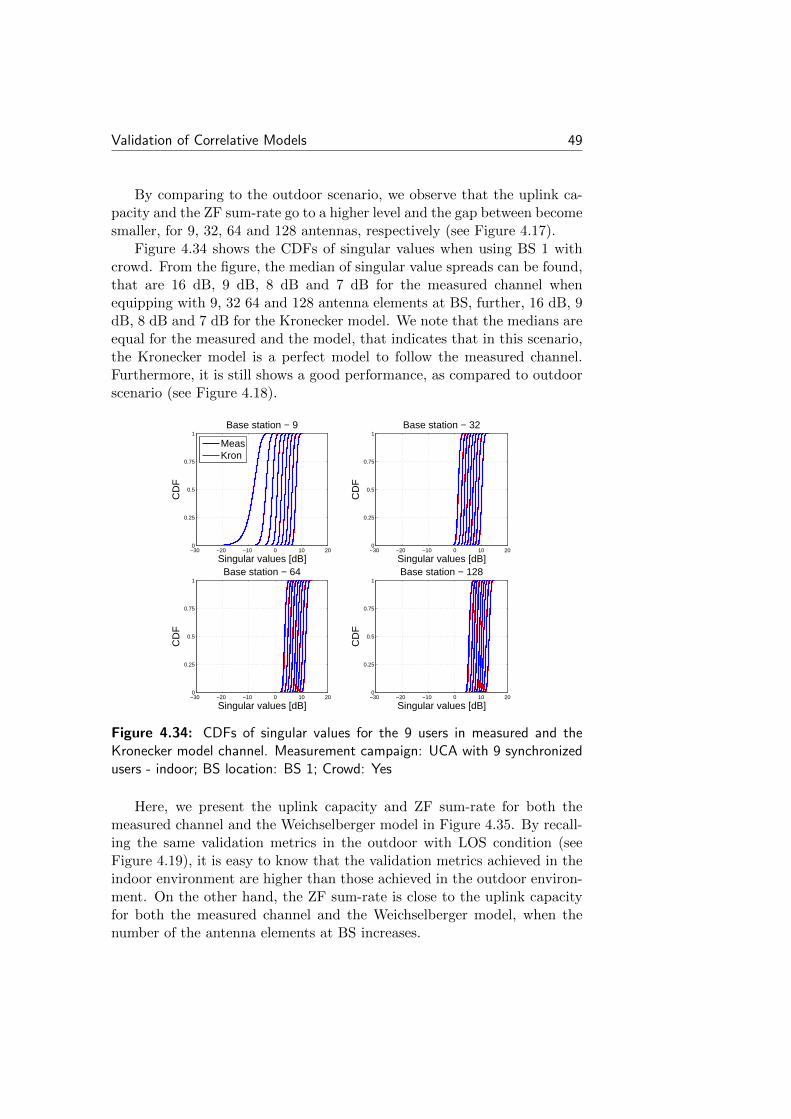
Validation of Correlative Models 49
By comparing to the outdoor scenario, we observe that the uplink ca-pacity and the ZF sum-rate go to a higher level and the gap between becomesmaller, for 9, 32, 64 and 128 antennas, respectively (see Figure 4.17).
Figure 4.34 shows the CDFs of singular values when using BS 1 withcrowd. From the figure, the median of singular value spreads can be found,that are 16 dB, 9 dB, 8 dB and 7 dB for the measured channel whenequipping with 9, 32 64 and 128 antenna elements at BS, further, 16 dB, 9dB, 8 dB and 7 dB for the Kronecker model. We note that the medians areequal for the measured and the model, that indicates that in this scenario,the Kronecker model is a perfect model to follow the measured channel.Furthermore, it is still shows a good performance, as compared to outdoorscenario (see Figure 4.18).
−30 −20 −10 0 10 200
0.25
0.5
0.75
1
Singular values [dB]
CD
F
Base station − 9
MeasKron
−30 −20 −10 0 10 200
0.25
0.5
0.75
1
Singular values [dB]
CD
F
Base station − 32
−30 −20 −10 0 10 200
0.25
0.5
0.75
1
Singular values [dB]
CD
F
Base station − 64
−30 −20 −10 0 10 200
0.25
0.5
0.75
1
Singular values [dB]
CD
F
Base station − 128
Figure 4.34: CDFs of singular values for the 9 users in measured and theKronecker model channel. Measurement campaign: UCA with 9 synchronizedusers - indoor; BS location: BS 1; Crowd: Yes
Here, we present the uplink capacity and ZF sum-rate for both themeasured channel and the Weichselberger model in Figure 4.35. By recall-ing the same validation metrics in the outdoor with LOS condition (seeFigure 4.19), it is easy to know that the validation metrics achieved in theindoor environment are higher than those achieved in the outdoor environ-ment. On the other hand, the ZF sum-rate is close to the uplink capacityfor both the measured channel and the Weichselberger model, when thenumber of the antenna elements at BS increases.

50 Validation of Correlative Models
−10 −5 0 5 100
5
10
15
20
25
30
Es/N
0 [dB]
Upl
ink
sum
−ra
te [b
ps/H
z]
Base station − 9
WeichWeich, ZFMeasMeas, ZF
−10 −5 0 5 100
5
10
15
20
25
30
Es/N
0 [dB]
Upl
ink
sum
−ra
te [b
ps/H
z]
Base station − 32
−10 −5 0 5 100
5
10
15
20
25
30
Es/N
0 [dB]
Upl
ink
sum
−ra
te [b
ps/H
z]
Base station − 64
−10 −5 0 5 100
5
10
15
20
25
30
Es/N
0 [dB]
Upl
ink
sum
−ra
te [b
ps/H
z]
Base station − 128
Figure 4.35: Validation of the Weichselberger model. Measurement cam-paign: UCA with 9 synchronized users - indoor; BS location: BS 1; Crowd:Yes.
−30 −20 −10 0 10 200
0.25
0.5
0.75
1
Singular values [dB]
CD
F
Base station − 9
MeasWeich
−30 −20 −10 0 10 200
0.25
0.5
0.75
1
Singular values [dB]
CD
F
Base station − 32
−30 −20 −10 0 10 200
0.25
0.5
0.75
1
Singular values [dB]
CD
F
Base station − 64
−30 −20 −10 0 10 200
0.25
0.5
0.75
1
Singular values [dB]
CD
F
Base station − 128
Figure 4.36: CDFs of singular values for the 9 users in measured and theWeichselberger model channel. Measurement campaign: UCA with 9 synchro-nized users - indoor; BS location: BS 1; Crowd: Yes
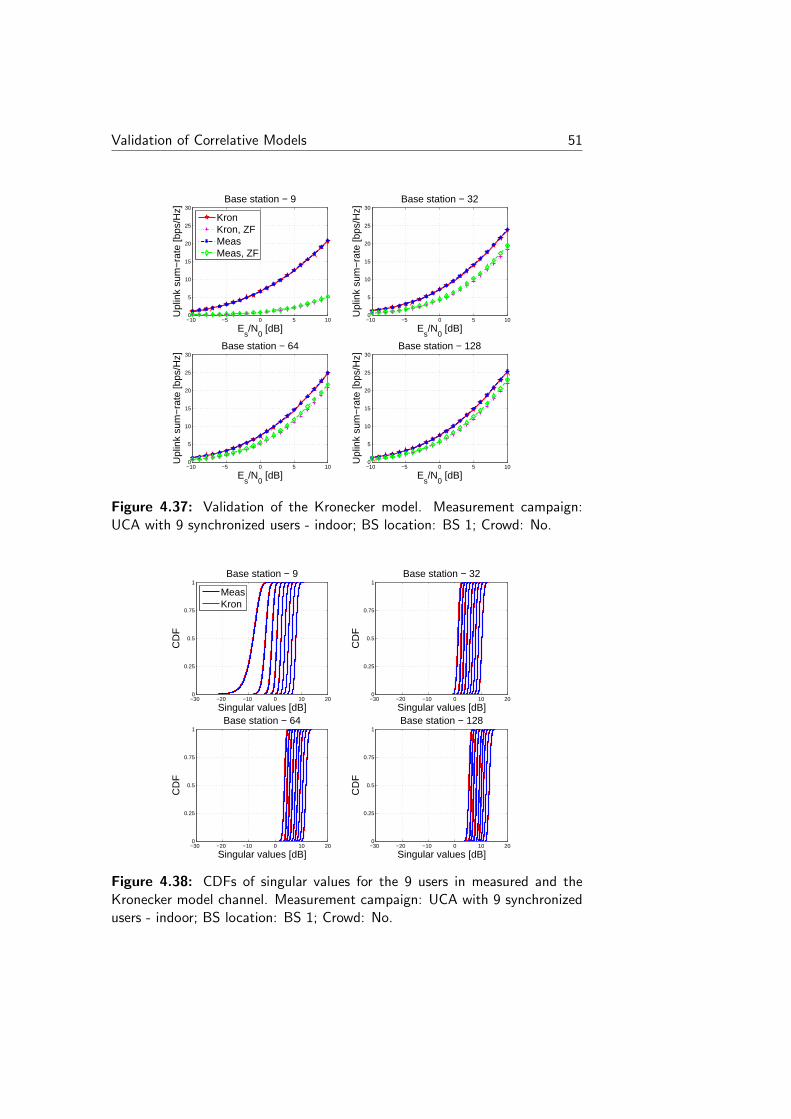
Validation of Correlative Models 51
−10 −5 0 5 100
5
10
15
20
25
30
Es/N
0 [dB]
Upl
ink
sum
−ra
te [b
ps/H
z]
Base station − 9
KronKron, ZFMeasMeas, ZF
−10 −5 0 5 100
5
10
15
20
25
30
Es/N
0 [dB]
Upl
ink
sum
−ra
te [b
ps/H
z]
Base station − 32
−10 −5 0 5 100
5
10
15
20
25
30
Es/N
0 [dB]
Upl
ink
sum
−ra
te [b
ps/H
z]
Base station − 64
−10 −5 0 5 100
5
10
15
20
25
30
Es/N
0 [dB]
Upl
ink
sum
−ra
te [b
ps/H
z]Base station − 128
Figure 4.37: Validation of the Kronecker model. Measurement campaign:UCA with 9 synchronized users - indoor; BS location: BS 1; Crowd: No.
−30 −20 −10 0 10 200
0.25
0.5
0.75
1
Singular values [dB]
CD
F
Base station − 9
MeasKron
−30 −20 −10 0 10 200
0.25
0.5
0.75
1
Singular values [dB]
CD
F
Base station − 32
−30 −20 −10 0 10 200
0.25
0.5
0.75
1
Singular values [dB]
CD
F
Base station − 64
−30 −20 −10 0 10 200
0.25
0.5
0.75
1
Singular values [dB]
CD
F
Base station − 128
Figure 4.38: CDFs of singular values for the 9 users in measured and theKronecker model channel. Measurement campaign: UCA with 9 synchronizedusers - indoor; BS location: BS 1; Crowd: No.
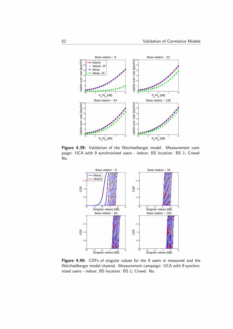
52 Validation of Correlative Models
−10 −5 0 5 100
5
10
15
20
25
30
Es/N
0 [dB]
Upl
ink
sum
−ra
te [b
ps/H
z]
Base station − 9
WeichWeich, ZFMeasMeas, ZF
−10 −5 0 5 100
5
10
15
20
25
30
Es/N
0 [dB]
Upl
ink
sum
−ra
te [b
ps/H
z]
Base station − 32
−10 −5 0 5 100
5
10
15
20
25
30
Es/N
0 [dB]
Upl
ink
sum
−ra
te [b
ps/H
z]
Base station − 64
−10 −5 0 5 100
5
10
15
20
25
30
Es/N
0 [dB]
Upl
ink
sum
−ra
te [b
ps/H
z]
Base station − 128
Figure 4.39: Validation of the Weichselberger model. Measurement cam-paign: UCA with 9 synchronized users - indoor; BS location: BS 1; Crowd:No.
−30 −20 −10 0 10 200
0.25
0.5
0.75
1
Singular values [dB]
CD
F
Base station − 9
MeasWeich
−30 −20 −10 0 10 200
0.25
0.5
0.75
1
Singular values [dB]
CD
F
Base station − 32
−30 −20 −10 0 10 200
0.25
0.5
0.75
1
Singular values [dB]
CD
F
Base station − 64
−30 −20 −10 0 10 200
0.25
0.5
0.75
1
Singular values [dB]
CD
F
Base station − 128
Figure 4.40: CDFs of singular values for the 9 users in measured and theWeichselberger model channel. Measurement campaign: UCA with 9 synchro-nized users - indoor; BS location: BS 1; Crowd: No.
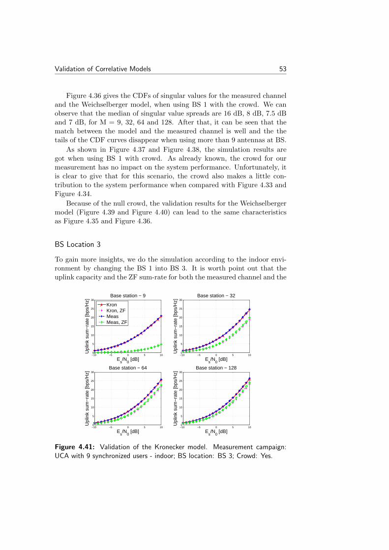
Validation of Correlative Models 53
Figure 4.36 gives the CDFs of singular values for the measured channeland the Weichselberger model, when using BS 1 with the crowd. We canobserve that the median of singular value spreads are 16 dB, 8 dB, 7.5 dBand 7 dB, for M = 9, 32, 64 and 128. After that, it can be seen that thematch between the model and the measured channel is well and the thetails of the CDF curves disappear when using more than 9 antennas at BS.
As shown in Figure 4.37 and Figure 4.38, the simulation results aregot when using BS 1 with crowd. As already known, the crowd for ourmeasurement has no impact on the system performance. Unfortunately, itis clear to give that for this scenario, the crowd also makes a little con-tribution to the system performance when compared with Figure 4.33 andFigure 4.34.
Because of the null crowd, the validation results for the Weichselbergermodel (Figure 4.39 and Figure 4.40) can lead to the same characteristicsas Figure 4.35 and Figure 4.36.
BS Location 3
To gain more insights, we do the simulation according to the indoor envi-ronment by changing the BS 1 into BS 3. It is worth point out that theuplink capacity and the ZF sum-rate for both the measured channel and the
−10 −5 0 5 100
5
10
15
20
25
30
Es/N
0 [dB]
Upl
ink
sum
−ra
te [b
ps/H
z]
Base station − 9
KronKron, ZFMeasMeas, ZF
−10 −5 0 5 100
5
10
15
20
25
30
Es/N
0 [dB]
Upl
ink
sum
−ra
te [b
ps/H
z]
Base station − 32
−10 −5 0 5 100
5
10
15
20
25
30
Es/N
0 [dB]
Upl
ink
sum
−ra
te [b
ps/H
z]
Base station − 64
−10 −5 0 5 100
5
10
15
20
25
30
Es/N
0 [dB]
Upl
ink
sum
−ra
te [b
ps/H
z]
Base station − 128
Figure 4.41: Validation of the Kronecker model. Measurement campaign:UCA with 9 synchronized users - indoor; BS location: BS 3; Crowd: Yes.
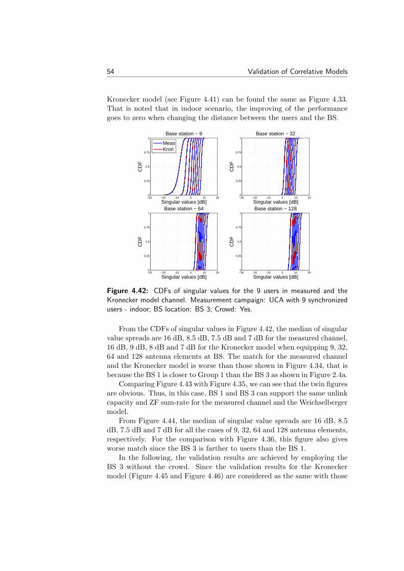
54 Validation of Correlative Models
Kronecker model (see Figure 4.41) can be found the same as Figure 4.33.That is noted that in indoor scenario, the improving of the performancegoes to zero when changing the distance between the users and the BS.
−30 −20 −10 0 10 200
0.25
0.5
0.75
1
Singular values [dB]
CD
FBase station − 9
MeasKron
−30 −20 −10 0 10 200
0.25
0.5
0.75
1
Singular values [dB]
CD
F
Base station − 32
−30 −20 −10 0 10 200
0.25
0.5
0.75
1
Singular values [dB]
CD
F
Base station − 64
−30 −20 −10 0 10 200
0.25
0.5
0.75
1
Singular values [dB]
CD
F
Base station − 128
Figure 4.42: CDFs of singular values for the 9 users in measured and theKronecker model channel. Measurement campaign: UCA with 9 synchronizedusers - indoor; BS location: BS 3; Crowd: Yes.
From the CDFs of singular values in Figure 4.42, the median of singularvalue spreads are 16 dB, 8.5 dB, 7.5 dB and 7 dB for the measured channel,16 dB, 9 dB, 8 dB and 7 dB for the Kronecker model when equipping 9, 32,64 and 128 antenna elements at BS. The match for the measured channeland the Kronecker model is worse than those shown in Figure 4.34, that isbecause the BS 1 is closer to Group 1 than the BS 3 as shown in Figure 2.4a.
Comparing Figure 4.43 with Figure 4.35, we can see that the twin figuresare obvious. Thus, in this case, BS 1 and BS 3 can support the same unlinkcapacity and ZF sum-rate for the measured channel and the Weichselbergermodel.
From Figure 4.44, the median of singular value spreads are 16 dB, 8.5dB, 7.5 dB and 7 dB for all the cases of 9, 32, 64 and 128 antenna elements,respectively. For the comparison with Figure 4.36, this figure also givesworse match since the BS 3 is farther to users than the BS 1.
In the following, the validation results are achieved by employing theBS 3 without the crowd. Since the validation results for the Kroneckermodel (Figure 4.45 and Figure 4.46) are considered as the same with those
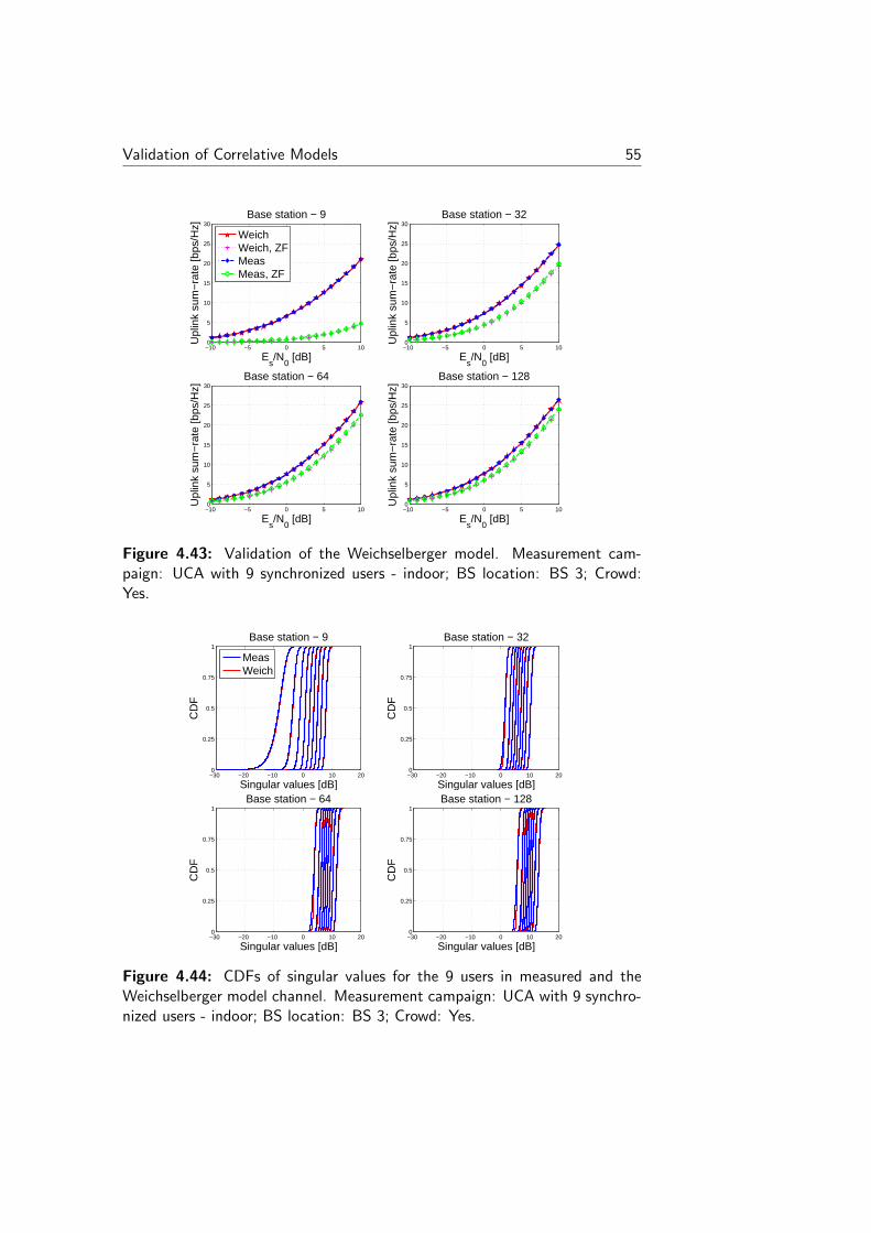
Validation of Correlative Models 55
−10 −5 0 5 100
5
10
15
20
25
30
Es/N
0 [dB]
Upl
ink
sum
−ra
te [b
ps/H
z]
Base station − 9
WeichWeich, ZFMeasMeas, ZF
−10 −5 0 5 100
5
10
15
20
25
30
Es/N
0 [dB]
Upl
ink
sum
−ra
te [b
ps/H
z]
Base station − 32
−10 −5 0 5 100
5
10
15
20
25
30
Es/N
0 [dB]
Upl
ink
sum
−ra
te [b
ps/H
z]
Base station − 64
−10 −5 0 5 100
5
10
15
20
25
30
Es/N
0 [dB]
Upl
ink
sum
−ra
te [b
ps/H
z]Base station − 128
Figure 4.43: Validation of the Weichselberger model. Measurement cam-paign: UCA with 9 synchronized users - indoor; BS location: BS 3; Crowd:Yes.
−30 −20 −10 0 10 200
0.25
0.5
0.75
1
Singular values [dB]
CD
F
Base station − 9
MeasWeich
−30 −20 −10 0 10 200
0.25
0.5
0.75
1
Singular values [dB]
CD
F
Base station − 32
−30 −20 −10 0 10 200
0.25
0.5
0.75
1
Singular values [dB]
CD
F
Base station − 64
−30 −20 −10 0 10 200
0.25
0.5
0.75
1
Singular values [dB]
CD
F
Base station − 128
Figure 4.44: CDFs of singular values for the 9 users in measured and theWeichselberger model channel. Measurement campaign: UCA with 9 synchro-nized users - indoor; BS location: BS 3; Crowd: Yes.
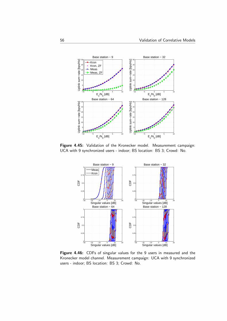
56 Validation of Correlative Models
−10 −5 0 5 100
5
10
15
20
25
30
Es/N
0 [dB]
Upl
ink
sum
−ra
te [b
ps/H
z]
Base station − 9
KronKron, ZFMeasMeas, ZF
−10 −5 0 5 100
5
10
15
20
25
30
Es/N
0 [dB]
Upl
ink
sum
−ra
te [b
ps/H
z]
Base station − 32
−10 −5 0 5 100
5
10
15
20
25
30
Es/N
0 [dB]
Upl
ink
sum
−ra
te [b
ps/H
z]
Base station − 64
−10 −5 0 5 100
5
10
15
20
25
30
Es/N
0 [dB]
Upl
ink
sum
−ra
te [b
ps/H
z]
Base station − 128
Figure 4.45: Validation of the Kronecker model. Measurement campaign:UCA with 9 synchronized users - indoor; BS location: BS 3; Crowd: No.
−30 −20 −10 0 10 200
0.25
0.5
0.75
1
Singular values [dB]
CD
F
Base station − 9
MeasKron
−30 −20 −10 0 10 200
0.25
0.5
0.75
1
Singular values [dB]
CD
F
Base station − 32
−30 −20 −10 0 10 200
0.25
0.5
0.75
1
Singular values [dB]
CD
F
Base station − 64
−30 −20 −10 0 10 200
0.25
0.5
0.75
1
Singular values [dB]
CD
F
Base station − 128
Figure 4.46: CDFs of singular values for the 9 users in measured and theKronecker model channel. Measurement campaign: UCA with 9 synchronizedusers - indoor; BS location: BS 3; Crowd: No.

Validation of Correlative Models 57
obtained in crowd (Figure 4.41 and Figure 4.42) and the validation resultsfor the Weichselberger model (see Figure 4.47 and Figure 4.48) also achievethe same validation results, as shown in Figure 4.43 and Figure 4.44, we donot give more comments for them.
−10 −5 0 5 100
5
10
15
20
25
30
Es/N
0 [dB]
Upl
ink
sum
−ra
te [b
ps/H
z]
Base station − 9
WeichWeich, ZFMeasMeas, ZF
−10 −5 0 5 100
5
10
15
20
25
30
Es/N
0 [dB]
Upl
ink
sum
−ra
te [b
ps/H
z]
Base station − 32
−10 −5 0 5 100
5
10
15
20
25
30
Es/N
0 [dB]
Upl
ink
sum
−ra
te [b
ps/H
z]
Base station − 64
−10 −5 0 5 100
5
10
15
20
25
30
Es/N
0 [dB]
Upl
ink
sum
−ra
te [b
ps/H
z]
Base station − 128
Figure 4.47: Validation of the Weichselberger model. Measurement cam-paign: UCA with 9 synchronized users - indoor; BS location: BS 3; Crowd:No.
In this chapter, we present an experimental analysis of the correlativechannel models by choosing typical scenarios, and validation results of allscenarios will be given in the Chapter 5. To the end, two comments tothe development of massive MIMO for this chapter can be summarized asfollows:
1. As already known, the crowd has no impact on the system perfor-mance and it is required to seek a good method to set the crowd ifwe want to investigate the influence of the crowd in the future.
2. Cylindrical array supports higher advantages than linear array.
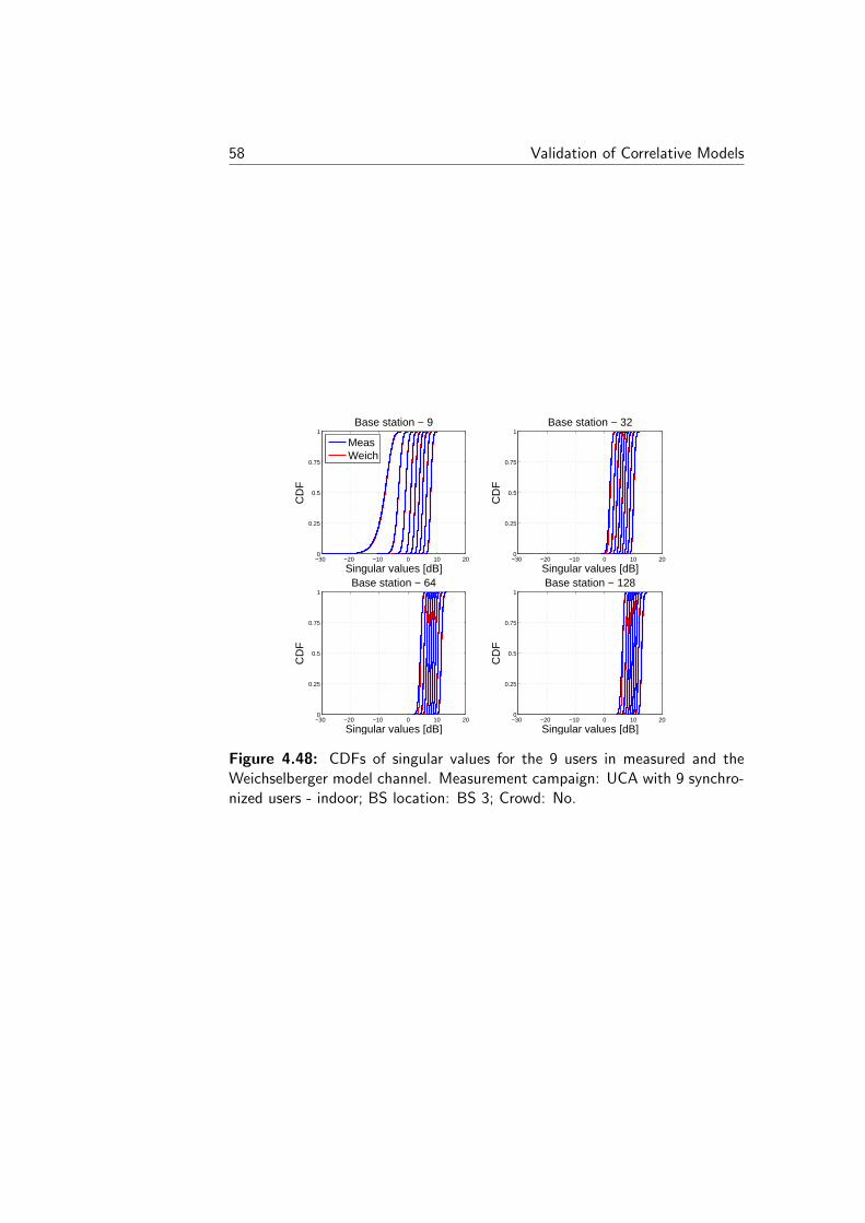
58 Validation of Correlative Models
−30 −20 −10 0 10 200
0.25
0.5
0.75
1
Singular values [dB]
CD
F
Base station − 9
MeasWeich
−30 −20 −10 0 10 200
0.25
0.5
0.75
1
Singular values [dB]
CD
F
Base station − 32
−30 −20 −10 0 10 200
0.25
0.5
0.75
1
Singular values [dB]
CD
F
Base station − 64
−30 −20 −10 0 10 200
0.25
0.5
0.75
1
Singular values [dB]
CD
F
Base station − 128
Figure 4.48: CDFs of singular values for the 9 users in measured and theWeichselberger model channel. Measurement campaign: UCA with 9 synchro-nized users - indoor; BS location: BS 3; Crowd: No.
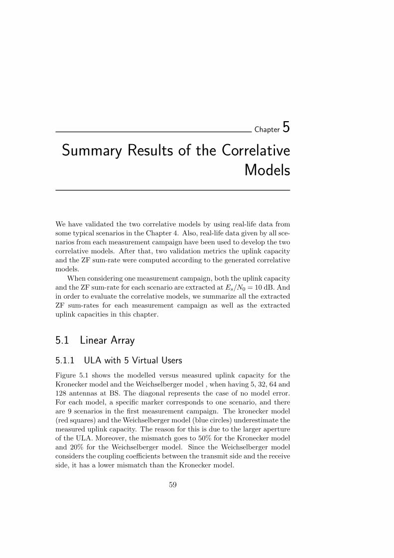
Chapter 5
Summary Results of the CorrelativeModels
We have validated the two correlative models by using real-life data fromsome typical scenarios in the Chapter 4. Also, real-life data given by all sce-narios from each measurement campaign have been used to develop the twocorrelative models. After that, two validation metrics the uplink capacityand the ZF sum-rate were computed according to the generated correlativemodels.
When considering one measurement campaign, both the uplink capacityand the ZF sum-rate for each scenario are extracted at Es/N0 = 10 dB. Andin order to evaluate the correlative models, we summarize all the extractedZF sum-rates for each measurement campaign as well as the extracteduplink capacities in this chapter.
5.1 Linear Array
5.1.1 ULA with 5 Virtual Users
Figure 5.1 shows the modelled versus measured uplink capacity for theKronecker model and the Weichselberger model , when having 5, 32, 64 and128 antennas at BS. The diagonal represents the case of no model error.For each model, a specific marker corresponds to one scenario, and thereare 9 scenarios in the first measurement campaign. The kronecker model(red squares) and the Weichselberger model (blue circles) underestimate themeasured uplink capacity. The reason for this is due to the larger apertureof the ULA. Moreover, the mismatch goes to 50% for the Kronecker modeland 20% for the Weichselberger model. Since the Weichselberger modelconsiders the coupling coefficients between the transmit side and the receiveside, it has a lower mismatch than the Kronecker model.
59
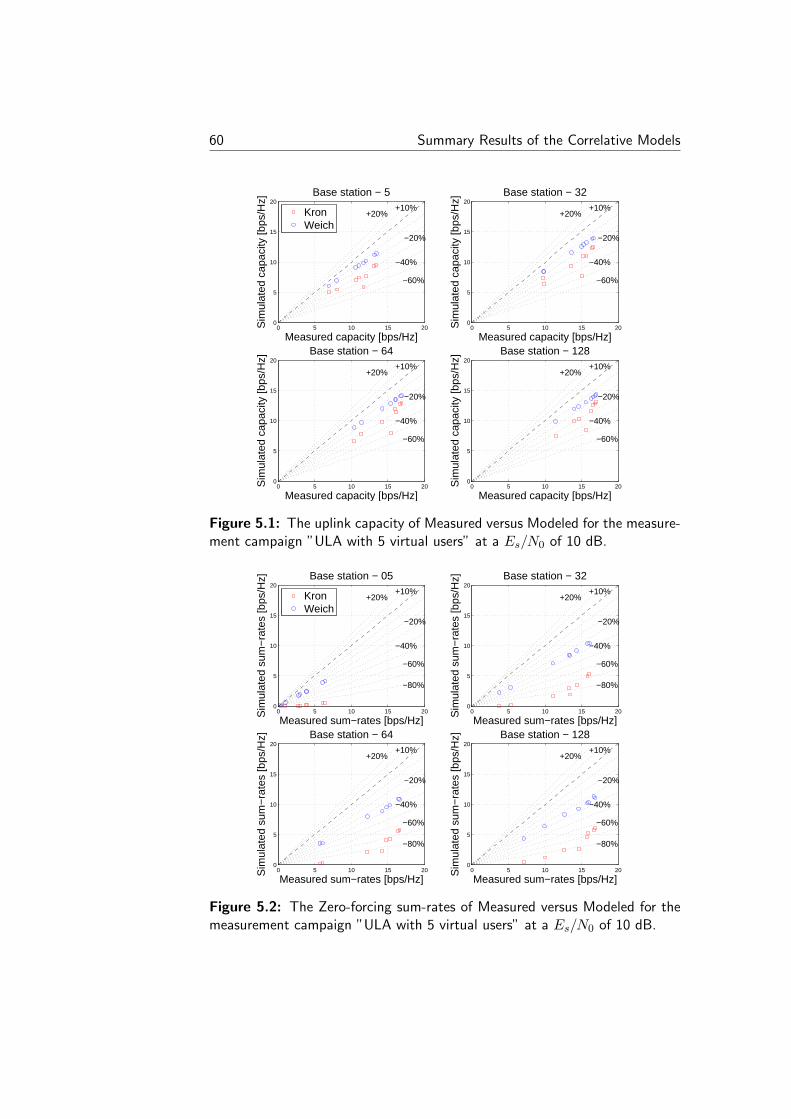
60 Summary Results of the Correlative Models
0 5 10 15 200
5
10
15
20+10%
+20%
−20%
−40%
−60%
Measured capacity [bps/Hz]
Sim
ulat
ed c
apac
ity [b
ps/H
z]
Base station − 5
KronWeich
0 5 10 15 200
5
10
15
20+10%
+20%
−20%
−40%
−60%
Measured capacity [bps/Hz]
Sim
ulat
ed c
apac
ity [b
ps/H
z]
Base station − 32
0 5 10 15 200
5
10
15
20+10%
+20%
−20%
−40%
−60%
Measured capacity [bps/Hz]
Sim
ulat
ed c
apac
ity [b
ps/H
z]
Base station − 64
0 5 10 15 200
5
10
15
20+10%
+20%
−20%
−40%
−60%
Measured capacity [bps/Hz]
Sim
ulat
ed c
apac
ity [b
ps/H
z]
Base station − 128
Figure 5.1: The uplink capacity of Measured versus Modeled for the measure-ment campaign ”ULA with 5 virtual users” at a Es/N0 of 10 dB.
0 5 10 15 200
5
10
15
20+10%
+20%
−20%
−40%
−60%
−80%
Measured sum−rates [bps/Hz]
Sim
ulat
ed s
um−
rate
s [b
ps/H
z] Base station − 05
KronWeich
0 5 10 15 200
5
10
15
20+10%
+20%
−20%
−40%
−60%
−80%
Measured sum−rates [bps/Hz]
Sim
ulat
ed s
um−
rate
s [b
ps/H
z] Base station − 32
0 5 10 15 200
5
10
15
20+10%
+20%
−20%
−40%
−60%
−80%
Measured sum−rates [bps/Hz]
Sim
ulat
ed s
um−
rate
s [b
ps/H
z] Base station − 64
0 5 10 15 200
5
10
15
20+10%
+20%
−20%
−40%
−60%
−80%
Measured sum−rates [bps/Hz]
Sim
ulat
ed s
um−
rate
s [b
ps/H
z] Base station − 128
Figure 5.2: The Zero-forcing sum-rates of Measured versus Modeled for themeasurement campaign ”ULA with 5 virtual users” at a Es/N0 of 10 dB.
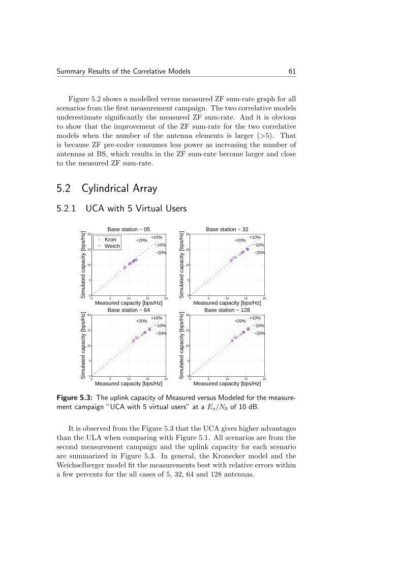
Summary Results of the Correlative Models 61
Figure 5.2 shows a modelled versus measured ZF sum-rate graph for allscenarios from the first measurement campaign. The two correlative modelsunderestimate significantly the measured ZF sum-rate. And it is obviousto show that the improvement of the ZF sum-rate for the two correlativemodels when the number of the antenna elements is larger (>5). Thatis because ZF pre-coder consumes less power as increasing the number ofantennas at BS, which results in the ZF sum-rate become larger and closeto the measured ZF sum-rate.
5.2 Cylindrical Array
5.2.1 UCA with 5 Virtual Users
0 5 10 15 200
5
10
15
20+10%
+20%−10%
−20%
Measured capacity [bps/Hz]
Sim
ulat
ed c
apac
ity [b
ps/H
z]
Base station − 05
KronWeich
0 5 10 15 200
5
10
15
20+10%
+20%−10%
−20%
Measured capacity [bps/Hz]
Sim
ulat
ed c
apac
ity [b
ps/H
z]
Base station − 32
0 5 10 15 200
5
10
15
20+10%
+20%−10%
−20%
Measured capacity [bps/Hz]
Sim
ulat
ed c
apac
ity [b
ps/H
z]
Base station − 64
0 5 10 15 200
5
10
15
20+10%
+20%−10%
−20%
Measured capacity [bps/Hz]
Sim
ulat
ed c
apac
ity [b
ps/H
z]
Base station − 128
Figure 5.3: The uplink capacity of Measured versus Modeled for the measure-ment campaign ”UCA with 5 virtual users” at a Es/N0 of 10 dB.
It is observed from the Figure 5.3 that the UCA gives higher advantagesthan the ULA when comparing with Figure 5.1. All scenarios are from thesecond measurement campaign and the uplink capacity for each scenarioare summarized in Figure 5.3. In general, the Kronecker model and theWeichselberger model fit the measurements best with relative errors withina few percents for the all cases of 5, 32, 64 and 128 antennas.

62 Summary Results of the Correlative Models
As with the scenarios from the second measurement campaign, the ZFsum-rates for all scenarios are shown in Figure 5.3. When considering 5antennas at BS, the Kronecker model error is 20% for all scenarios, whereasthat of the Weichselberger model is 5%. However, when having more than5 antennas, the ZF sum-rate for both models improve significantly and thetwo correlative models error remains relatively constant regardless of arraysize.
For the second measurement campaign, note that for all scenarios, boththe uplink capacity and the ZF sum-rate extend to a longer interval, ashaving more antennas at BS (>5). As mentioned in Chapter 4, the envi-ronment for this measurement campaign fluctuates rapidly, that leads tothe extension for the uplink capacity and the ZF sum-rate.
0 5 10 15 200
5
10
15
20+10%
+20%−10%
−20%
Measured sum−rates [bps/Hz]
Sim
ulat
ed s
um−
rate
s [b
ps/H
z] Base station − 05
KronWeich
0 5 10 15 200
5
10
15
20+10%
+20%−10%
−20%
Measured sum−rates [bps/Hz]
Sim
ulat
ed s
um−
rate
s [b
ps/H
z] Base station − 32
0 5 10 15 200
5
10
15
20+10%
+20%−10%
−20%
Measured sum−rates [bps/Hz]
Sim
ulat
ed s
um−
rate
s [b
ps/H
z] Base station − 64
0 5 10 15 200
5
10
15
20+10%
+20%−10%
−20%
Measured sum−rates [bps/Hz]
Sim
ulat
ed s
um−
rate
s [b
ps/H
z] Base station − 128
Figure 5.4: The Zero-forcing sum-rates of Measured versus Modeled for themeasurement campaign ”UCA with 5 virtual users” at a Es/N0 of 10 dB.
5.2.2 UCA with 9 Synchronized Users - Outdoor
In Figure 5.5, the modelled versus measured uplink capacity for all scenarioslisted in the third measurement campaign is shown. The Kronecker modeland the Weichselberger model perform quite well overall for equipping 9,32, 64 and 128 antennas at BS. The two correlative models error for allscenarios shows almost zero and remains zero regardless of array size.
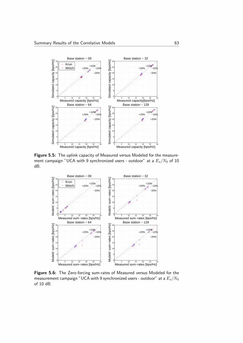
Summary Results of the Correlative Models 63
0 5 10 15 20 25 300
5
10
15
20
25
30
+10%+20% −10%
−20%
Measured capacity [bps/Hz]
Sim
ulat
ed c
apac
ity [b
ps/H
z]
Base station − 09
KronWeich
0 5 10 15 20 25 300
5
10
15
20
25
30
+10%+20% −10%
−20%
Measured capacity[bps/Hz]
Sim
ulat
ed c
apac
ity [b
ps/H
z]
Base station − 32
0 5 10 15 20 25 300
5
10
15
20
25
30
+10%+20% −10%
−20%
Measured capacity [bps/Hz]
Sim
ulat
ed c
apac
ity [b
ps/H
z]
Base station − 64
0 5 10 15 20 25 300
5
10
15
20
25
30
+10%+20% −10%
−20%
Measured capacity [bps/Hz]
Sim
ulat
ed c
apac
ity [b
ps/H
z]Base station − 128
Figure 5.5: The uplink capacity of Measured versus Modeled for the measure-ment campaign ”UCA with 9 synchronized users - outdoor” at a Es/N0 of 10dB.
0 5 10 15 20 25 300
5
10
15
20
25
30
+10%+20% −10%
−20%
Measured sum−rates [bps/Hz]
Mod
els’
sum
−ra
tes
[bps
/Hz]
Base station − 09
KronWeich
0 5 10 15 20 25 300
5
10
15
20
25
30
+10%+20% −10%
−20%
Measured sum−rates [bps/Hz]
Mod
els’
sum
−ra
tes
[bps
/Hz]
Base station − 32
0 5 10 15 20 25 300
5
10
15
20
25
30
+10%+20% −10%
−20%
Measured sum−rates [bps/Hz]
Mod
els’
sum
−ra
tes
[bps
/Hz]
Base station − 64
0 5 10 15 20 25 300
5
10
15
20
25
30
+10%+20% −10%
−20%
Measured sum−rates [bps/Hz]
Mod
els’
sum
−ra
tes
[bps
/Hz]
Base station − 128
Figure 5.6: The Zero-forcing sum-rates of Measured versus Modeled for themeasurement campaign ”UCA with 9 synchronized users - outdoor” at a Es/N0
of 10 dB.
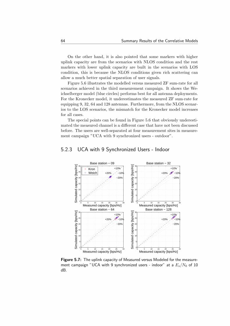
64 Summary Results of the Correlative Models
On the other hand, it is also pointed that some markers with higheruplink capacity are from the scenarios with NLOS condition and the restmarkers with lower uplink capacity are built in the scenarios with LOScondition, this is because the NLOS conditions given rich scattering canallow a much better spatial separation of user signals.
Figure 5.6 illustrates the modelled versus measured ZF sum-rate for allscenarios achieved in the third measurement campaign. It shows the We-ichselberger model (blue circles) performs best for all antenna deployments.For the Kronecker model, it underestimates the measured ZF sum-rate forequipping 9, 32, 64 and 128 antennas. Furthermore, from the NLOS scenar-ios to the LOS scenarios, the mismatch for the Kronecker model increasesfor all cases.
The special points can be found in Figure 5.6 that obviously underesti-mated the measured channel is a different case that have not been discussedbefore. The users are well-separated at four measurement sites in measure-ment campaign ”UCA with 9 synchronized users - outdoor”.
5.2.3 UCA with 9 Synchronized Users - Indoor
0 5 10 15 20 25 300
5
10
15
20
25
30
+10%
+20% −10%
−20%
Measured capacity [bps/Hz]
Sim
ulat
ed c
apac
ity [b
ps/H
z]
Base station − 09
KronWeich
0 5 10 15 20 25 300
5
10
15
20
25
30
+10%
+20% −10%
−20%
Measured capacity [bps/Hz]
Sim
ulat
ed c
apac
ity [b
ps/H
z]
Base station − 32
0 5 10 15 20 25 300
5
10
15
20
25
30
+10%
+20% −10%
−20%
Measured capacity [bps/Hz]
Sim
ulat
ed c
apac
ity [b
ps/H
z]
Base station − 64
0 5 10 15 20 25 300
5
10
15
20
25
30
+10%
+20% −10%
−20%
Measured capacity [bps/Hz]
Sim
ulat
ed c
apac
ity [b
ps/H
z]
Base station − 128
Figure 5.7: The uplink capacity of Measured versus Modeled for the measure-ment campaign ”UCA with 9 synchronized users - indoor” at a Es/N0 of 10dB.
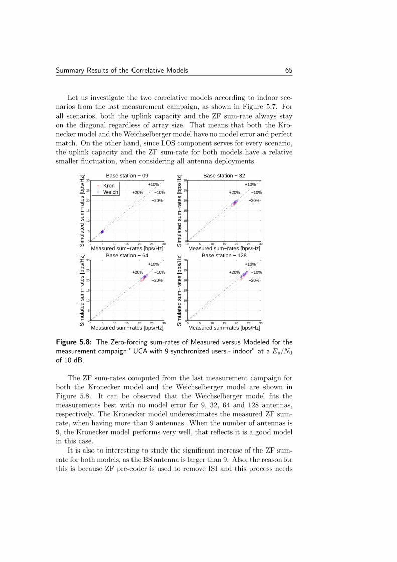
Summary Results of the Correlative Models 65
Let us investigate the two correlative models according to indoor sce-narios from the last measurement campaign, as shown in Figure 5.7. Forall scenarios, both the uplink capacity and the ZF sum-rate always stayon the diagonal regardless of array size. That means that both the Kro-necker model and the Weichselberger model have no model error and perfectmatch. On the other hand, since LOS component serves for every scenario,the uplink capacity and the ZF sum-rate for both models have a relativesmaller fluctuation, when considering all antenna deployments.
0 5 10 15 20 25 300
5
10
15
20
25
30
+10%
+20% −10%
−20%
Measured sum−rates [bps/Hz]
Sim
ulat
ed s
um−
rate
s [b
ps/H
z] Base station − 09
KronWeich
0 5 10 15 20 25 300
5
10
15
20
25
30
+10%
+20% −10%
−20%
Measured sum−rates [bps/Hz]
Sim
ulat
ed s
um−
rate
s [b
ps/H
z] Base station − 32
0 5 10 15 20 25 300
5
10
15
20
25
30
+10%
+20% −10%
−20%
Measured sum−rates [bps/Hz]
Sim
ulat
ed s
um−
rate
s [b
ps/H
z] Base station − 64
0 5 10 15 20 25 300
5
10
15
20
25
30
+10%
+20% −10%
−20%
Measured sum−rates [bps/Hz]
Sim
ulat
ed s
um−
rate
s [b
ps/H
z] Base station − 128
Figure 5.8: The Zero-forcing sum-rates of Measured versus Modeled for themeasurement campaign ”UCA with 9 synchronized users - indoor” at a Es/N0
of 10 dB.
The ZF sum-rates computed from the last measurement campaign forboth the Kronecker model and the Weichselberger model are shown inFigure 5.8. It can be observed that the Weichselberger model fits themeasurements best with no model error for 9, 32, 64 and 128 antennas,respectively. The Kronecker model underestimates the measured ZF sum-rate, when having more than 9 antennas. When the number of antennas is9, the Kronecker model performs very well, that reflects it is a good modelin this case.
It is also to interesting to study the significant increase of the ZF sum-rate for both models, as the BS antenna is larger than 9. Also, the reason forthis is because ZF pre-coder is used to remove ISI and this process needs

66 Summary Results of the Correlative Models
to consume power, however, the consumption reduces, as the number ofantenna elements at BS increases.
In the end, two comments for this chapter are given by
• Firstly, in the literature [15], it has been shown that the Kroneckermodel performs poorly, when having larger antennas (>3). However,the Kronercker model shows good match for equipping more antennasat BS, when considering UCA scenarios.
• Second, for massive MIMO channels performed with UCA, both theKronverker model and the Weichselberger are good model for perfor-mance analysis and evaluation.

Chapter 6
Random Cluster Model
To model the massive MIMO channel based on the Random Cluster Model(RCM) [16], we use the measurement data from the measurement campaign”ULA with 5 virtual users” with the linear array. In this chapter, themeasurement data processing, the implementation of the RCM as well asthe channel behavior and validation will be present.
6.1 Measurement Data Processing
Instead of investigating the measured channel matrix, i.e., the correlativemodels, the RCM is modeled on a cluster level. The space-alternatinggeneralized expectation maximization(SAGE) algorithm [23] is applied toestimate the MPCs of the raw data obtained from the measurement. Withjoint clustering and tracking, the MPCs having similar azimuth angles,elevation angles and delays are grouped into one cluster by using KPower-Means clustering algorithm [24]. To extract the clusters better, a slidingwindow with 10 adjacent antennas over the ULA was implemented.
6.2 Parametric Model
Each of the extracted clusters contains a set of parameters to classify thecluster location, power, spread, number of the MPCs in each cluster andits updating over time. The impulse response of the channel can be writtenas the sum of the cluster impulse responses:
H(t, f) =
Nc∑c=1
Hc(t, f,Θc) (6.1)
where Hc expresses the impulse response of the cth cluster, the clusterparameter set Θc contains the mean azimuth and elevation angles for both
67
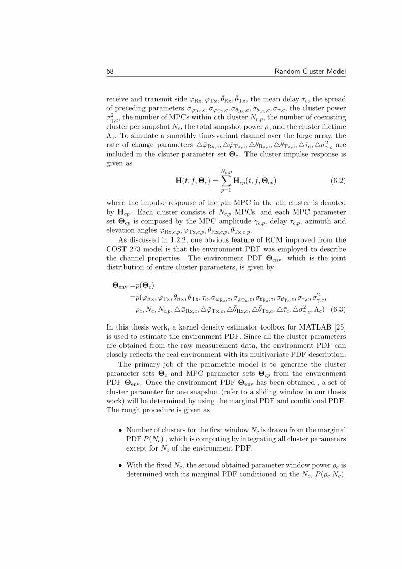
68 Random Cluster Model
receive and transmit side ϕRx, ϕTx, θRx, θTx, the mean delay τc, the spreadof preceding parameters σϕRx,c, σϕTx,c, σθRx,c, σθTx,c, στ,c, the cluster powerσ2γ,c, the number of MPCs within cth cluster Nc,p, the number of coexistingcluster per snapshot Nc, the total snapshot power ρc and the cluster lifetimeΛc. To simulate a smoothly time-variant channel over the large array, therate of change parameters 4ϕRx,c,4ϕTx,c,4θRx,c,4θTx,c,4τc,4σ2γ,c areincluded in the clsuter parameter set Θc. The cluster impulse response isgiven as
H(t, f,Θc) =
Nc,p∑p=1
Hcp(t, f,Θcp) (6.2)
where the impulse response of the pth MPC in the cth cluster is denotedby Hcp. Each cluster consists of Nc,p MPCs, and each MPC parameterset Θcp is composed by the MPC amplitude γc,p, delay τc,p, azimuth andelevation angles ϕRx,c,p, ϕTx,c,p, θRx,c,p, θTx,c,p.
As discussed in 1.2.2, one obvious feature of RCM improved from theCOST 273 model is that the environment PDF was employed to describethe channel properties. The environment PDF Θenv, which is the jointdistribution of entire cluster parameters, is given by
Θenv =p(Θc)
=p(ϕRx, ϕTx, θRx, θTx, τc, σϕRx,c, σϕTx,c, σθRx,c, σθTx,c, στ,c, σ2γ,c,
ρc, Nc, Nc,p,4ϕRx,c,4ϕTx,c,4θRx,c,4θTx,c,4τc,4σ2γ,c,Λc) (6.3)
In this thesis work, a kernel density estimator toolbox for MATLAB [25]is used to estimate the environment PDF. Since all the cluster parametersare obtained from the raw measurement data, the environment PDF canclosely reflects the real environment with its multivariate PDF description.
The primary job of the parametric model is to generate the clusterparameter sets Θc and MPC parameter sets Θcp from the environmentPDF Θenv. Once the environment PDF Θenv has been obtained , a set ofcluster parameter for one snapshot (refer to a sliding window in our thesiswork) will be determined by using the marginal PDF and conditional PDF.The rough procedure is given as
• Number of clusters for the first windowNc is drawn from the marginalPDF P (Nc) , which is computing by integrating all cluster parametersexcept for Nc of the environment PDF.
• With the fixed Nc, the second obtained parameter window power ρc isdetermined with its marginal PDF conditioned on the Nc, P (ρc|Nc).
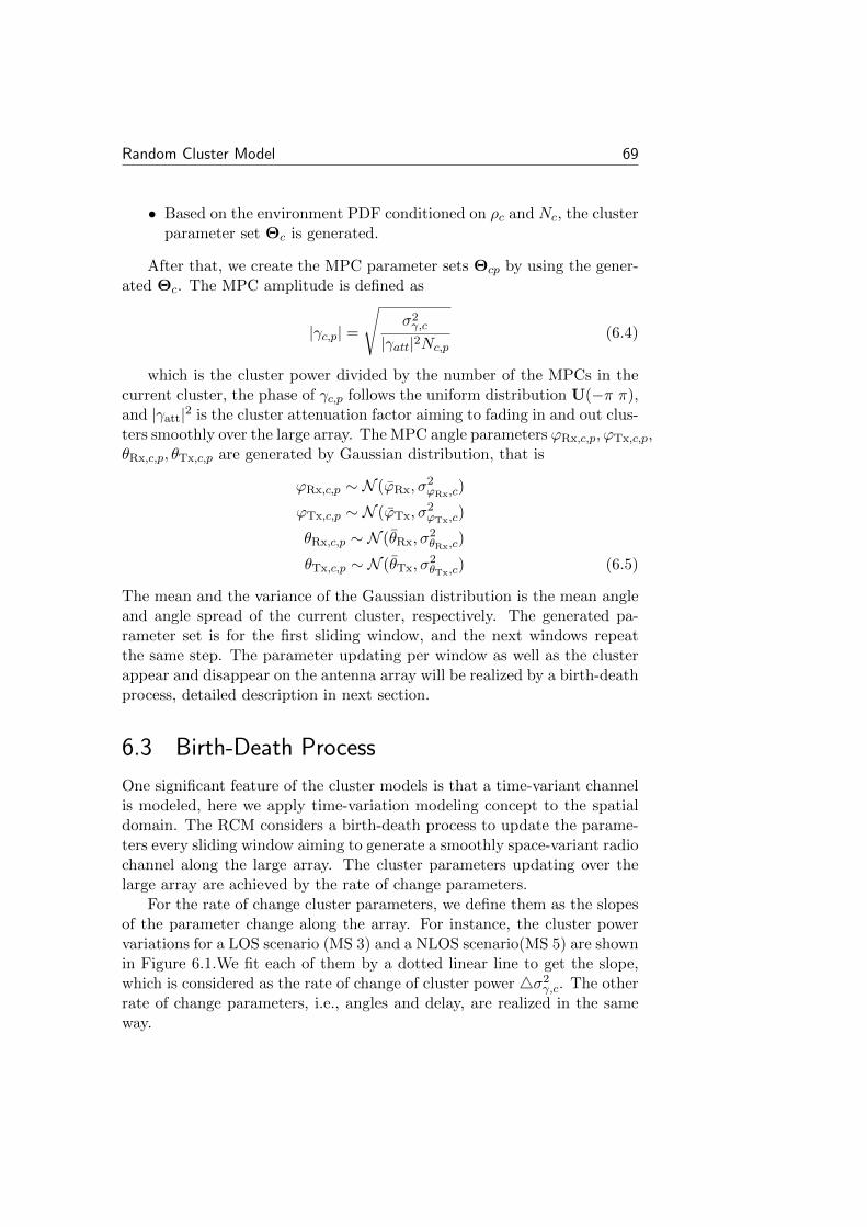
Random Cluster Model 69
• Based on the environment PDF conditioned on ρc and Nc, the clusterparameter set Θc is generated.
After that, we create the MPC parameter sets Θcp by using the gener-ated Θc. The MPC amplitude is defined as
|γc,p| =
√σ2γ,c
|γatt|2Nc,p(6.4)
which is the cluster power divided by the number of the MPCs in thecurrent cluster, the phase of γc,p follows the uniform distribution U(−π π),and |γatt|2 is the cluster attenuation factor aiming to fading in and out clus-ters smoothly over the large array. The MPC angle parameters ϕRx,c,p, ϕTx,c,p,θRx,c,p, θTx,c,p are generated by Gaussian distribution, that is
ϕRx,c,p ∼ N (ϕRx, σ2ϕRx,c
)
ϕTx,c,p ∼ N (ϕTx, σ2ϕTx,c
)
θRx,c,p ∼ N (θRx, σ2θRx,c
)
θTx,c,p ∼ N (θTx, σ2θTx,c
) (6.5)
The mean and the variance of the Gaussian distribution is the mean angleand angle spread of the current cluster, respectively. The generated pa-rameter set is for the first sliding window, and the next windows repeatthe same step. The parameter updating per window as well as the clusterappear and disappear on the antenna array will be realized by a birth-deathprocess, detailed description in next section.
6.3 Birth-Death Process
One significant feature of the cluster models is that a time-variant channelis modeled, here we apply time-variation modeling concept to the spatialdomain. The RCM considers a birth-death process to update the parame-ters every sliding window aiming to generate a smoothly space-variant radiochannel along the large array. The cluster parameters updating over thelarge array are achieved by the rate of change parameters.
For the rate of change cluster parameters, we define them as the slopesof the parameter change along the array. For instance, the cluster powervariations for a LOS scenario (MS 3) and a NLOS scenario(MS 5) are shownin Figure 6.1.We fit each of them by a dotted linear line to get the slope,which is considered as the rate of change of cluster power 4σ2γ,c. The otherrate of change parameters, i.e., angles and delay, are realized in the sameway.
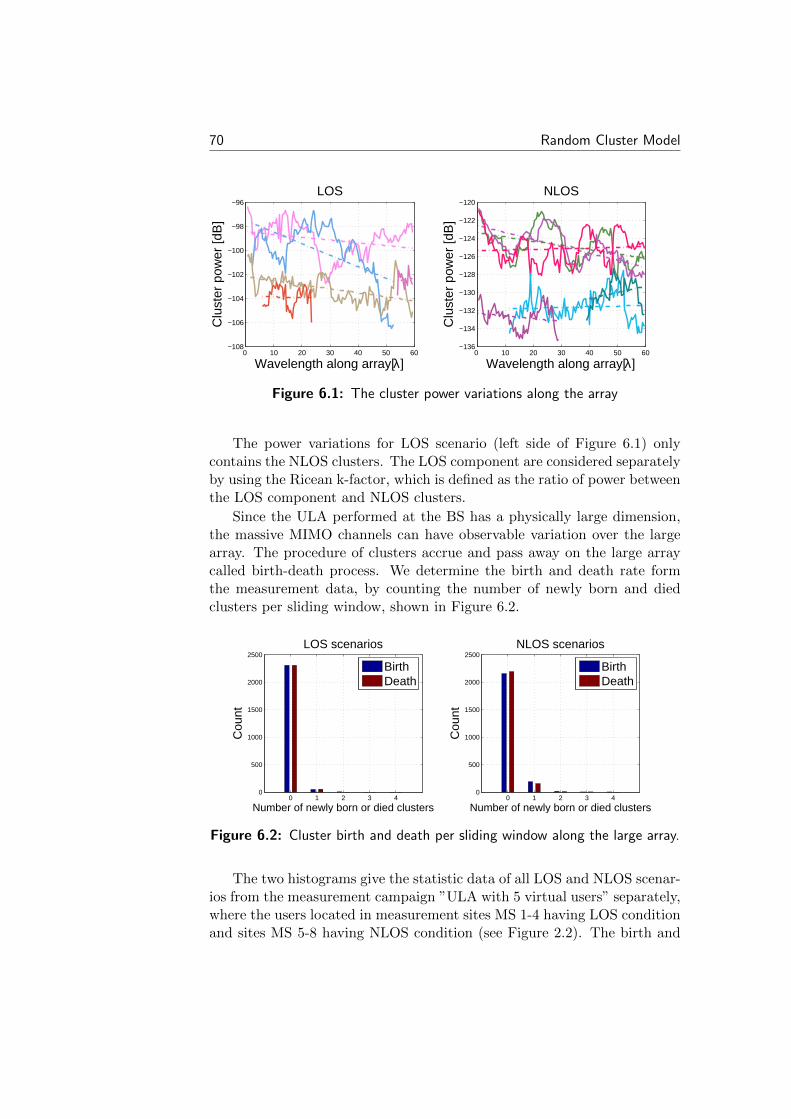
70 Random Cluster Model
0 10 20 30 40 50 60−108
−106
−104
−102
−100
−98
−96
Wavelength along array[λ]
Clu
ster
pow
er [d
B]
LOS
0 10 20 30 40 50 60−136
−134
−132
−130
−128
−126
−124
−122
−120
Wavelength along array[λ]
Clu
ster
pow
er [d
B]
NLOS
Figure 6.1: The cluster power variations along the array
The power variations for LOS scenario (left side of Figure 6.1) onlycontains the NLOS clusters. The LOS component are considered separatelyby using the Ricean k-factor, which is defined as the ratio of power betweenthe LOS component and NLOS clusters.
Since the ULA performed at the BS has a physically large dimension,the massive MIMO channels can have observable variation over the largearray. The procedure of clusters accrue and pass away on the large arraycalled birth-death process. We determine the birth and death rate formthe measurement data, by counting the number of newly born and diedclusters per sliding window, shown in Figure 6.2.
0 1 2 3 40
500
1000
1500
2000
2500
Number of newly born or died clusters
Cou
nt
LOS scenarios
BirthDeath
0 1 2 3 40
500
1000
1500
2000
2500
Number of newly born or died clusters
Cou
nt
NLOS scenarios
BirthDeath
Figure 6.2: Cluster birth and death per sliding window along the large array.
The two histograms give the statistic data of all LOS and NLOS scenar-ios from the measurement campaign ”ULA with 5 virtual users” separately,where the users located in measurement sites MS 1-4 having LOS conditionand sites MS 5-8 having NLOS condition (see Figure 2.2). The birth and
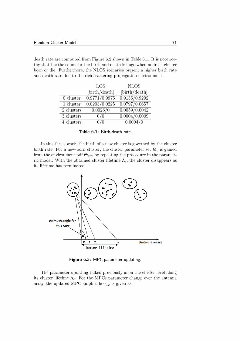
Random Cluster Model 71
death rate are computed from Figure 6.2 shown in Table 6.1. It is notewor-thy that the the count for the birth and death is huge when no fresh clusterborn or die. Furthermore, the NLOS scenarios present a higher birth rateand death rate due to the rich scattering propagation environment.
LOS NLOS[birth/death] [birth/death]
0 cluster 0.9771/0.9975 0.9136/0.92921 cluster 0.0203/0.0225 0.0797/0.06572 clusters 0.0026/0 0.0059/0.00423 clusters 0/0 0.0004/0.00094 clusters 0/0 0.0004/0
Table 6.1: Birth-death rate.
In this thesis work, the birth of a new cluster is governed by the clusterbirth rate. For a new-born cluster, the cluster parameter set Θc is gainedfrom the environment pdf Θenv by repeating the procedure in the paramet-ric model. With the obtained cluster lifetime Λc, the cluster disappears asits lifetime has terminated.
Figure 6.3: MPC parameter updating.
The parameter updating talked previously is on the cluster level alongits cluster lifetime Λc. For the MPCs parameter change over the antennaarray, the updated MPC amplitude γc,p is given as

72 Random Cluster Model
|γn+1c,p |2 = |γnc,p|2 +4σ2γ,c
λ
2(6.6)
where 4σ2γ,c is the rate of change of cluster power, λ2 is the distance of twoadjacent antenna element. The MPC delay τc,p is refreshed by establishinga coordinate system (see Figure 6.3). The MPC position is representedby its coordinate (cosϕRx,c,pdc,p, sinϕRx,c,pdc,p). And dc,p is the distancebetween the MPC and the BS array, which is calculated by multiplyingthe MPC delay τc,p by the speed of light. And the ϕRx,c,p is the azimuthangle at receiver side obtained in Section 6.2. After given the coordinateof the MPC, the dc,p can be determined for the each antenna consisted inits lifetime.
6.4 System Model
According to the cluster parameters and MPC parameters generated before,the system model can be written as
H(t, f) =
Nc∑c=1
Nc,p∑p=1
γc,paRx(ϕRx, θRx)aTTx(ϕTx, θTx)e−j2πfτc,p (6.7)
where aRx(ϕRx, θRx) is the receive array steering vector and aTx(ϕTx, θTx)is the transmit array steering vector. And Nc, Nc,p are the number of thecluster per snapshot and the number of MPCs in cth cluster, respectively.τc,p is the delay for each MPC in cth cluster. Here we have omni-directionalantennas at the BS, the array steering vector equals to 1. And the phasedifferent was embodied in the MPCs delay updating. We can rewrite thesystem model as
H(t, f) =
Nc∑c=1
Nc,p∑p=1
γc,pe−j2πfτc,p (6.8)
For the LOS scenario simulation, the direct propagation path LOS compo-nent achieved by Ricean k-factor is considered as a special cluster consistedof only one MPC, and the lifetime Λc of the LOS cluster is assumed as thewhole linear array.
6.5 Model Validation
To validate the simulated model, a number of scalar properties showingthe channel performance are introduced, i.e., the spatial and statistic auto-
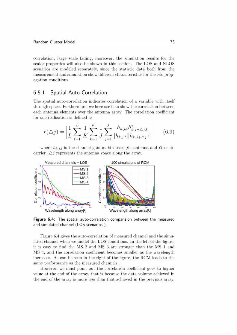
Random Cluster Model 73
correlation, large scale fading, moreover, the simulation results for thescalar properties will also be shown in this section. The LOS and NLOSscenarios are modeled separately, since the statistic data both from themeasurement and simulation show different characteristics for the two prop-agation conditions.
6.5.1 Spatial Auto-Correlation
The spatial auto-correlation indicates correlation of a variable with itselfthrough space. Furthermore, we here use it to show the correlation betweeneach antenna elements over the antenna array. The correlation coefficientfor one realization is defined as
r(4j) =
∣∣∣∣∣ 1LL∑`=1
1
K
K∑k=1
1
J
J∑j=1
hk,j,`h∗k,j+4j,`
|hk,j,`||hk,j+4j,`|
∣∣∣∣∣ (6.9)
where hk,j,` is the channel gain at kth user, jth antenna and `th sub-carrier. 4j represents the antenna space along the array.
0 10 20 30 40 50 600
0.2
0.4
0.6
0.8
1
Wavelength along array[λ]
Cor
rela
tion
coef
ficie
nt
Measured channels − LOS
MS 1MS 2MS 3MS 4
0 10 20 30 40 50 600
0.2
0.4
0.6
0.8
1
Wavelength along array[λ]
Cor
rela
tion
coef
ficie
nt
100 simulations of RCM
Figure 6.4: The spatial auto-correlation comparision between the measuredand simulated channel (LOS scenarios ).
Figure 6.4 gives the auto-correlation of measured channel and the simu-lated channel when we model the LOS conditions. In the left of the figure,it is easy to find the MS 2 and MS 3 are stronger than the MS 1 andMS 4, and the correlation coefficient becomes smaller as the wavelengthincreases. As can be seen in the right of the figure, the RCM leads to thesame performance as the measured channels.
However, we must point out the correlation coefficient goes to highervalue at the end of the array, that is because the data volume achieved inthe end of the array is more less than that achieved in the previous array.

74 Random Cluster Model
0 10 20 30 40 50 600
0.2
0.4
0.6
0.8
1
Wavelength along array[λ]
Cor
rela
tion
coef
ficie
nt
Measured channels − NLOS
MS 5MS 6MS 7MS 8
0 10 20 30 40 50 600
0.2
0.4
0.6
0.8
1
Wavelength along array[λ]
Cor
rela
tion
coef
ficie
nt
100 simulations of RCM
Figure 6.5: The spatial auto-correlation comparision between the measuredand simulated channel (NLOS scenarios ).
On the other hand, the simulation times is not enough due to the timeconstraints.
0 10 20 30 40 50 600
0.2
0.4
0.6
0.8
1
Wavelength along array[λ]
Cor
rela
tion
coef
ficie
nt
LOS scenarios
Measured channelSimulated channel
0 10 20 30 40 50 600
0.2
0.4
0.6
0.8
1
Wavelength along array[λ]
Cor
rela
tion
coef
ficie
nt
NLOS scenarios
Measured channelSimulated channel
Figure 6.6: The averaged spatial auto-correlation comparision between themeasured and simulated channel.
According to the left of Figure 6.5, we can see that the correlation coeffi-cient for the NLOS conditions always goes to smaller after a few wavelengthif consider the measured channels, since the scatterers in the environmentcan support strong decorrelation effect to the channel. The same charac-teristics is given for the model channel, as illustrated in the right of thefigure. As mentioned in the last paragraph, the simulation times for thisare also not enough.
In the Figure 6.6 we plot the average spatial auto-correlation of theLOS scenarios and the NLOS scenarios for the measured channel and thesimulated channel. Both the LOS scenarios and the NLOS scenarios showa smaller gap between the measured channel and the simulated channel.
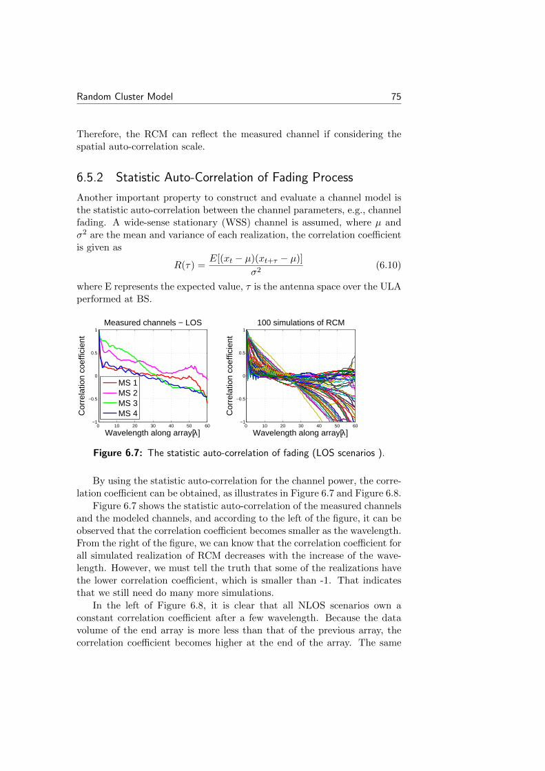
Random Cluster Model 75
Therefore, the RCM can reflect the measured channel if considering thespatial auto-correlation scale.
6.5.2 Statistic Auto-Correlation of Fading Process
Another important property to construct and evaluate a channel model isthe statistic auto-correlation between the channel parameters, e.g., channelfading. A wide-sense stationary (WSS) channel is assumed, where µ andσ2 are the mean and variance of each realization, the correlation coefficientis given as
R(τ) =E[(xt − µ)(xt+τ − µ)]
σ2(6.10)
where E represents the expected value, τ is the antenna space over the ULAperformed at BS.
0 10 20 30 40 50 60−1
−0.5
0
0.5
1
Wavelength along array[λ]
Cor
rela
tion
coef
ficie
nt
Measured channels − LOS
MS 1MS 2MS 3MS 4
0 10 20 30 40 50 60−1
−0.5
0
0.5
1
Wavelength along array[λ]
Cor
rela
tion
coef
ficie
nt
100 simulations of RCM
Figure 6.7: The statistic auto-correlation of fading (LOS scenarios ).
By using the statistic auto-correlation for the channel power, the corre-lation coefficient can be obtained, as illustrates in Figure 6.7 and Figure 6.8.
Figure 6.7 shows the statistic auto-correlation of the measured channelsand the modeled channels, and according to the left of the figure, it can beobserved that the correlation coefficient becomes smaller as the wavelength.From the right of the figure, we can know that the correlation coefficient forall simulated realization of RCM decreases with the increase of the wave-length. However, we must tell the truth that some of the realizations havethe lower correlation coefficient, which is smaller than -1. That indicatesthat we still need do many more simulations.
In the left of Figure 6.8, it is clear that all NLOS scenarios own aconstant correlation coefficient after a few wavelength. Because the datavolume of the end array is more less than that of the previous array, thecorrelation coefficient becomes higher at the end of the array. The same
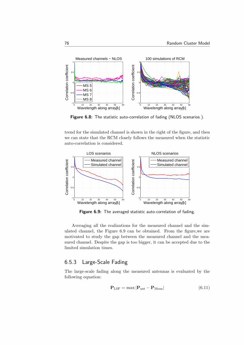
76 Random Cluster Model
0 10 20 30 40 50 60−1
−0.5
0
0.5
1
Wavelength along array[λ]
Cor
rela
tion
coef
ficie
nt
Measured channels − NLOS
MS 5MS 6MS 7MS 8
0 10 20 30 40 50 60−1
−0.5
0
0.5
1
Wavelength along array[λ]
Cor
rela
tion
coef
ficie
nt
100 simulations of RCM
Figure 6.8: The statistic auto-correlation of fading (NLOS scenarios ).
trend for the simulated channel is shown in the right of the figure, and thenwe can state that the RCM closely follows the measured when the statisticauto-correlation is considered.
0 10 20 30 40 50 60−1
−0.5
0
0.5
1
Wavelength along array[λ]
Cor
rela
tion
coef
ficie
nt
LOS scenarios
Measured channelSimulated channel
0 10 20 30 40 50 60−1
−0.5
0
0.5
1
Wavelength along array[λ]
Cor
rela
tion
coef
ficie
nt
NLOS scenarios
Measured channelSimulated channel
Figure 6.9: The averaged statistic auto-correlation of fading.
Averaging all the realizations for the measured channel and the sim-ulated channel, the Figure 6.9 can be obtained. From the figure,we aremotivated to study the gap between the measured channel and the mea-sured channel. Despite the gap is too bigger, it can be accepted due to thelimited simulation times.
6.5.3 Large-Scale Fading
The large-scale fading along the measured antennas is evaluated by thefollowing equation:
PLSF = max |Pant −PMean| (6.11)
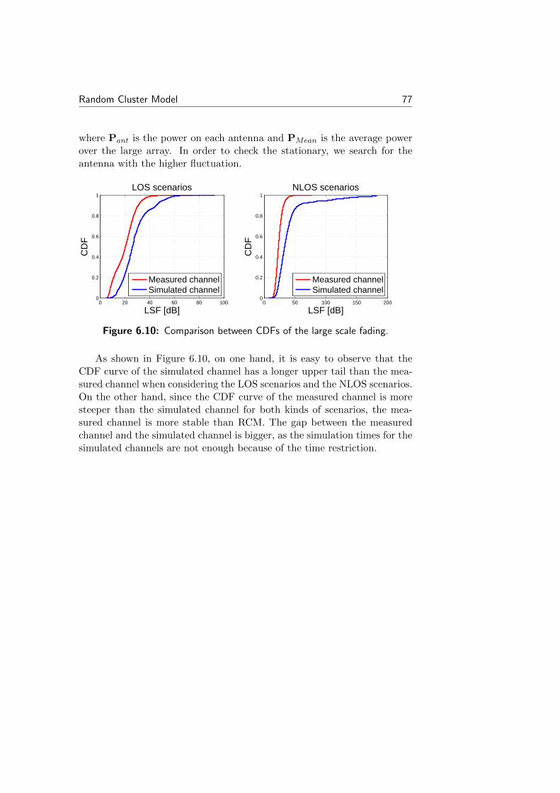
Random Cluster Model 77
where Pant is the power on each antenna and PMean is the average powerover the large array. In order to check the stationary, we search for theantenna with the higher fluctuation.
0 20 40 60 80 1000
0.2
0.4
0.6
0.8
1
LSF [dB]
CD
F
LOS scenarios
Measured channelSimulated channel
0 50 100 150 2000
0.2
0.4
0.6
0.8
1
LSF [dB]
CD
F
NLOS scenarios
Measured channelSimulated channel
Figure 6.10: Comparison between CDFs of the large scale fading.
As shown in Figure 6.10, on one hand, it is easy to observe that theCDF curve of the simulated channel has a longer upper tail than the mea-sured channel when considering the LOS scenarios and the NLOS scenarios.On the other hand, since the CDF curve of the measured channel is moresteeper than the simulated channel for both kinds of scenarios, the mea-sured channel is more stable than RCM. The gap between the measuredchannel and the simulated channel is bigger, as the simulation times for thesimulated channels are not enough because of the time restriction.

78 Random Cluster Model
Chapter 7
Conclusions and Discussion
This thesis has investigated the correlative models and the cluster modelfor massive MIMO by using measured channels.
Conclusion and summary for the correlative models are as follows:
• With physically-large array, both the uplink capacity and the ZFsum-rates achieved in the correlative models underestimate thoseachieved in the real-life channel. Furthermore, the Weichselbergermodel is more accurate than the Kronecker model. Singular valuespreads were gathered for different scenarios, and they indicates thatthe correlative models cannot do a good job of representing the real-life channel. The worse match is because of the physically large array.
• With compact cylindrical array and closely-spaced users, we deliverseveral conclusions for the correlative models, that is, (i) the cor-relative models match well with real-life data. (ii) Both the uplinkcapacity and the ZF sum-rate not only are influenced by rapidlychanging environment (following the second measured campaign),but also give higher values for the LOS scenarios when comparedwith NLOS scenarios (following the third measurement campaign).(iii) We found that for compact array and closely-spaced users, thecorrelative models can be used for analytical study and the furtherproblem is that large number of parameters in correlation matrix isa modelling challenge.
To the end, the RCM employed a statistical description (namely en-vironment PDF) of the measured scenarios to generate clusters for themodelled scenario. Expect for that, we used the Birth-death process tomodel continuously time-varying scenarios and used the K-factor to modelthe LOS component.
In order to validate the RCM, the spatial auto-correlation, the statisticauto-correlation and the large-scale fading have been examined. Despite
79

80 Conclusions and Discussion
the spatial auto-correlation has shown that the channel correlation give agood match between the RCM and the measured channels, the statisticauto-correlation and the large-scale fading told us that the power matchstill needs to improve. On the other hand, the simulation times is notenough due to the time constraints.
In future work, it is interesting to consider well-separated users, wheninvestigating the correlative models. And for the RCM, we may do enoughsimulations so that some better suggestions can be achieved.
References
[1] X. Gao, O. Edfors, F. Rusek, and F. Tufvesson, “Linear pre-codingperformance in measured very-large MIMO channels,” in IEEE Vehic-ular Technology Conference (VTC Fall), Sep. 2011.
[2] E. Dahlman, S. Parkvall, J. Skold, and P. Beming, 3G Evolution, Sec-ond Edition: HSPA and LTE for Mobile Broadband, 2nd ed. AcademicPress, 2008.
[3] T. Narasimhan, P. Raviteja, and A. Chockalingam, “Large-scale mul-tiuser SM-MIMO versus massive MIMO,” in Information Theory andApplications Workshop(ITA), Feb. 2014.
[4] J. Hoydis, S. ten Brink, and M. Debbah, “Massive MIMO in theUL/DL of cellular networks: How many antennas do we need ?” IEEEJournal on Selected Areas in Communications, Feb. 2013.
[5] R. Baldemair, E. Dahlman, G. Fodor, G. Mildh, S. Parkvall, Y. Se-len, H. Tullberg, and K. Balachandran, “Evolving wireless communi-cations: Addressing the challenges and expectations of the future,”IEEE Vehicular Technology Magazine, Mar. 2013.
[6] E. Larsson, O. Edfors, F. Tufvesson, and T. Marzetta, “Massive MIMOfor next generation wireless systems,” IEEE Communications Maga-zine, Feb. 2014.
[7] F. Boccardi, R. Heath, A. Lozano, T. Marzetta, and P. Popovski,“Five disruptive technology directions for 5G,” IEEE CommunicationsMagazine, Feb. 2014.
[8] H. Q. Ngo, “Massive MIMO: Fundamentals and system designs,”Ph.D. dissertation, Linkoping University, 2015.
81

82 References
[9] D. Tse and P. Viswanath, Fundamentals of Wireless Communication.New York,USA: Cambridge University Press, 2005.
[10] H. Q. Ngo, E. Larsson, and T. Marzetta, “Energy and spectral effi-ciency of very large multiuser MIMO systems,” IEEE Transactions onCommunications, Apr. 2013.
[11] F. Rusek, D. Persson, B. K. Lau, E. Larsson, T. Marzetta, O. Edfors,and F. Tufvesson, “Scaling up MIMO: Opportunities and challengeswith very large arrays,” IEEE Signal Processing Magazine, Jan. 2013.
[12] S. Wyne, A. Molisch, P. Almers, G. Eriksson, J. Karedal, andF. Tufvesson, “Statistical evaluation of outdoor-to-indoor office MIMOmeasurements at 5.2 GHz,” in IEEE VTC-Spring, May 2005.
[13] N. Costa and S. Haykin, Multiple-input, multiple-output channel mod-els: theory and practice, ser. Wiley series in adaptive and learning sys-tems for signal processing, communication and control. New York:IEEE, Institute of Electrical and Electronic Engineers Hoboken, N.J.John Wiley, 2010.
[14] W. Weichselberger, M. Herdin, H. Ozcelik, and E. Bonek, “A stochas-tic MIMO channel model with joint correlation of both link ends,”IEEE Transactions on Wireless Communications, Jan. 2006.
[15] W. Weichselberger, “Spatial structure of multiple antenna radio chan-nels a signal processing viewpoint,” Ph.D. dissertation, TechnischeUniversitat Wien, Dec. 2003.
[16] N. Czink, “The random-cluster model - a stochastic MIMO channelmodel for broadband wireless communication systems of the 3rd gener-ation and beyond,” Ph.D. dissertation, Technische Universitat Wien,2007.
[17] X. Gao, O. Edfors, F. Rusek, and F. Tufvesson, “Massive MIMOperformance evaluation based on measured propagation data,” IEEETransactions on Wireless Communications, July 2015.
[18] X. Gao, F. Tufvesson, O. Edfors, and F. Rusek, “Measured propaga-tion characteristics for very-large MIMO at 2.6 GHz,” in ConferenceRecord of the 46th Asilomar Conference on Signals, Systems and Com-puters (ASILOMAR), Nov. 2012.
[19] “D1.2 - MaMi channel characteristics: Measurement results,”ULUND, Report, 2015.
References 83
[20] J. Flordelis, X. Gao, G. Dahman, F. Rusek, O. Edfors, and F. Tufves-son, “Spatial separation of closely-spaced users in measured massivemulti-user MIMO channels,” in IEEE International Conference onCommunications, 2015.
[21] A. Paulraj, R. Nabar, and D. Gore, Introduction to Space-Time Wire-less Communications, 1st ed. New York,USA: Cambridge UniversityPress, 2003.
[22] X. Gao, M. Zhu, F. Rusek, F. Tufvesson, and O. Edfors, “Large an-tenna array and propagation environment interaction,” in 48th Asilo-mar Conference on Signals, Systems and Computers, Nov. 2014.
[23] B. Fleury, M. Tschudin, R. Heddergott, D. Dahlhaus, and K. Inge-man Pedersen, “Channel parameter estimation in mobile radio envi-ronments using the SAGE algorithm,” IEEE Journal on Selected Areasin Communications, Mar. 1999.
[24] N. Czink, P. Cera, J. Salo, E. Bonek, J.-P. Nuutinen, and J. Ylitalo,“A framework for automatic clustering of parametric MIMO channeldata including path powers,” in IEEE 64th Vehicular Technology Con-ference, Sep. 2006.
[25] A. Ihler, “Kernel density estimation toolbox for MATLAB,”http://www.ics.uci.edu/ ihler/code/kde.html, July 2007.

84 References

List of Figures
1.1 Transmit correlation only depends on the scattering at thetransmit side, and correspondingly, receive correlation only re-lies on the scattering at the receive side. . . . . . . . . . . . . 4
1.2 The RCM framework . . . . . . . . . . . . . . . . . . . . . . 5
2.1 Two large antenna arrays: a) practical uniform cylindrical array(UCA), and b) virtual uniform linear array (ULA). . . . . . . 8
2.2 Overview of the measurement area at the campus of the Facultyof Engineering (LTH), Lund University, Sweden. Two BS largeantenna arrays were placed at the same roof of E-building ofLTH during the two respective measurement campaigns, 8 MSsites were measured. . . . . . . . . . . . . . . . . . . . . . . 9
2.3 UCA with 9 synchronized users - outdoor measurement (a) Themeasurement area, (b) The users moving randomly in a 5 mdiameter circle. . . . . . . . . . . . . . . . . . . . . . . . . . 10
2.4 UCA with 9 synchronized users - indoor measurement (a) Themeasurement area, (b) The users. . . . . . . . . . . . . . . . 11
3.1 The transmit-correlation matrix (left) and the receive-correlationmatrix (right). Measurement campaign: ULA with 5 virtualusers; User location: MS 2; Propagation condition: LOS. . . . 14
3.2 The transmit-correlation matrix (left) and the receive-correlationmatrix (right). Measurement campaign: ULA with 5 virtualusers; User location: MS 5; Propagation condition: NLOS. . . 15
4.1 Validation of the Kronecker model. Measurement campaign:ULA with 5 virtual users; User location: MS 2; Propagationcondition: LOS. . . . . . . . . . . . . . . . . . . . . . . . . . 23
85
86 LIST OF FIGURES
4.2 CDFs of singular values for the 5 users in measured and theKronecker model channel. Measurement campaign: ULA with5 virtual users; User location: MS 2; Propagation condition:LOS. . . . . . . . . . . . . . . . . . . . . . . . . . . . . . . . 24
4.3 Validation of the Weichselberger model. Measurement cam-paign: ULA with 5 virtual users; User location: MS 2; Propa-gation condition: LOS. . . . . . . . . . . . . . . . . . . . . . 24
4.4 CDFs of singular values for the 5 users in measured and theWeichselberger model channel. Measurement campaign: ULAwith 5 virtual users; User location: MS 2; Propagation condi-tion: LOS. . . . . . . . . . . . . . . . . . . . . . . . . . . . . 25
4.5 Validation of the Kronecker model. Measurement campaign:ULA with 5 virtual users; User location: MS 5; Propagationcondition: NLOS. . . . . . . . . . . . . . . . . . . . . . . . . 26
4.6 CDFs of singular values for the 5 users in measured and theKronecker model channel. Measurement campaign: ULA with5 virtual users; User location: MS 5; Propagation condition:NLOS. . . . . . . . . . . . . . . . . . . . . . . . . . . . . . . 27
4.7 Validation of the Weichselberger model. Measurement cam-paign: ULA with 5 virtual users; User location: MS 5; Propa-gation condition: NLOS. . . . . . . . . . . . . . . . . . . . . 28
4.8 CDFs of singular values for the 5 users in measured and theWeichselberger model channel. Measurement campaign: ULAwith 5 virtual users; User location: MS 5; Propagation condi-tion: NLOS. . . . . . . . . . . . . . . . . . . . . . . . . . . . 28
4.9 Validation of the Kronecker model. Measurement campaign:UCA with 5 virtual users; User location: MS 2; Propagationcondition: LOS. . . . . . . . . . . . . . . . . . . . . . . . . 30
4.10 CDFs of singular values for the 5 users in measured and theKronecker model channel. Measurement campaign: UCA with5 virtual users; User location: MS 2; Propagation condition:LOS. . . . . . . . . . . . . . . . . . . . . . . . . . . . . . . . 31
4.11 Validation of the Weichselberger model. Measurement cam-paign: UCA with 5 virtual users; User location: MS 2; Propa-gation condition: LOS. . . . . . . . . . . . . . . . . . . . . . 32
4.12 CDFs of singular values for the 5 users in measured and theWeichselberger model channel. Measurement campaign: UCAwith 5 virtual users; User location: MS 2; Propagation condi-tion: LOS. . . . . . . . . . . . . . . . . . . . . . . . . . . . . 32
LIST OF FIGURES 87
4.13 Validation of the Kronecker model. Measurement campaign:UCA with 5 virtual users; User location: MS 5; Propagationcondition: NLOS . . . . . . . . . . . . . . . . . . . . . . . . 33
4.14 CDFs of singular values for the 5 users in measured and theKronecker model channel. Measurement campaign: UCA with5 virtual users; User location: MS 5; Propagation condition:NLOS. . . . . . . . . . . . . . . . . . . . . . . . . . . . . . . 34
4.15 Validation of the Weichselberger model. Measurement cam-paign: UCA with 5 virtual users; User location: MS 5; Propa-gation condition: NLOS . . . . . . . . . . . . . . . . . . . . 35
4.16 CDFs of singular values for the 5 users in measured and theWeichselberger model channel. Measurement campaign: UCAwith 5 virtual users; User location: MS 5; Propagation condi-tion: NLOS. . . . . . . . . . . . . . . . . . . . . . . . . . . . 35
4.17 Validation of the Kronecker model. Measurement campaign:UCA with 9 synchronized users - outdoor; User location: MS1; Propagation condition: LOS - Crowd. . . . . . . . . . . . . 37
4.18 CDFs of singular values for the 9 users in measured and theKronecker model channel. Measurement campaign: UCA with9 synchronized users - outdoor; User location: MS 1; Propa-gation condition: LOS - Crowd. . . . . . . . . . . . . . . . . 37
4.19 Validation of the Weichselberger model. Measurement cam-paign: UCA with 9 synchronized users - outdoor; User location:MS 1; Propagation condition: LOS - Crowd. . . . . . . . . . 38
4.20 CDFs of singular values for the 9 users in measured and theWeichselberger model channel. Measurement campaign: UCAwith 9 synchronized users - outdoor; User location: MS 1;Propagation condition: LOS - Crowd. . . . . . . . . . . . . . 39
4.21 Validation of the Kronecker model. Measurement campaign:UCA with 9 synchronized users - outdoor; User location: MS1; Propagation condition: LOS - No Crowd. . . . . . . . . . . 40
4.22 CDFs of singular values for the 9 users in measured and theKronecker model channel. Measurement campaign: UCA with9 synchronized users - outdoor; User location: MS 1; Propa-gation condition: LOS - No Crowd. . . . . . . . . . . . . . . 40
4.23 Validation of the Weichselberger model. Measurement cam-paign: UCA with 9 synchronized users - outdoor; User location:MS 1; Propagation condition: LOS - No Crowd. . . . . . . . 41
88 LIST OF FIGURES
4.24 CDFs of singular values for the 9 users in measured and theWeichselberger model channel. Measurement campaign: UCAwith 9 synchronized users - outdoor; User location: MS 1;Propagation condition: LOS - No Crowd. . . . . . . . . . . . 42
4.25 Validation of the Kronecker model. Measurement campaign:UCA with 9 synchronized users - outdoor; User location: MS3; Propagation condition: NLOS - Crowd. . . . . . . . . . . . 43
4.26 CDFs of singular values for the 9 users in measured and theKronecker model channel. Measurement campaign: UCA with9 synchronized users - outdoor; User location: MS 3; Propa-gation condition: NLOS - Crowd. . . . . . . . . . . . . . . . 43
4.27 Validation of the Weichselberger model. Measurement cam-paign: UCA with 9 synchronized users - outdoor; User location:MS 3; Propagation condition: NLOS - Crowd. . . . . . . . . 44
4.28 CDFs of singular values for the 9 users in measured and theWeichselberger model channel. Measurement campaign: UCAwith 9 synchronized users - outdoor; User location: MS 3;Propagation condition: NLOS - Crowd. . . . . . . . . . . . . 45
4.29 Validation of the Kronecker model. Measurement campaign:UCA with 9 synchronized users - outdoor; User location: MS3; Propagation condition: NLOS - No Crowd. . . . . . . . . . 45
4.30 CDFs of singular values for the 9 users in measured and theKronecker model channel. Measurement campaign: UCA with9 synchronized users - outdoor; User location: MS 3; Propa-gation condition: NLOS - No Crowd. . . . . . . . . . . . . . 46
4.31 Validation of the Weichselberger model. Measurement cam-paign: UCA with 9 synchronized users - outdoor; User location:MS 3; Propagation condition: NLOS - No Crowd. . . . . . . 47
4.32 CDFs of singular values for the 9 users in measured and theWeichselberger model channel. Measurement campaign: UCAwith 9 synchronized users - outdoor; User location: MS 3;Propagation condition: NLOS - No Crowd. . . . . . . . . . . 47
4.33 Validation of the Kronecker model. Measurement campaign:UCA with 9 synchronized users - indoor; BS location: BS 1;Crowd: Yes. . . . . . . . . . . . . . . . . . . . . . . . . . . . 48
4.34 CDFs of singular values for the 9 users in measured and theKronecker model channel. Measurement campaign: UCA with9 synchronized users - indoor; BS location: BS 1; Crowd: Yes 49
4.35 Validation of the Weichselberger model. Measurement cam-paign: UCA with 9 synchronized users - indoor; BS location:BS 1; Crowd: Yes. . . . . . . . . . . . . . . . . . . . . . . . 50
LIST OF FIGURES 89
4.36 CDFs of singular values for the 9 users in measured and theWeichselberger model channel. Measurement campaign: UCAwith 9 synchronized users - indoor; BS location: BS 1; Crowd:Yes . . . . . . . . . . . . . . . . . . . . . . . . . . . . . . . 50
4.37 Validation of the Kronecker model. Measurement campaign:UCA with 9 synchronized users - indoor; BS location: BS 1;Crowd: No. . . . . . . . . . . . . . . . . . . . . . . . . . . . 51
4.38 CDFs of singular values for the 9 users in measured and theKronecker model channel. Measurement campaign: UCA with9 synchronized users - indoor; BS location: BS 1; Crowd: No. 51
4.39 Validation of the Weichselberger model. Measurement cam-paign: UCA with 9 synchronized users - indoor; BS location:BS 1; Crowd: No. . . . . . . . . . . . . . . . . . . . . . . . . 52
4.40 CDFs of singular values for the 9 users in measured and theWeichselberger model channel. Measurement campaign: UCAwith 9 synchronized users - indoor; BS location: BS 1; Crowd:No. . . . . . . . . . . . . . . . . . . . . . . . . . . . . . . . 52
4.41 Validation of the Kronecker model. Measurement campaign:UCA with 9 synchronized users - indoor; BS location: BS 3;Crowd: Yes. . . . . . . . . . . . . . . . . . . . . . . . . . . . 53
4.42 CDFs of singular values for the 9 users in measured and theKronecker model channel. Measurement campaign: UCA with9 synchronized users - indoor; BS location: BS 3; Crowd: Yes. 54
4.43 Validation of the Weichselberger model. Measurement cam-paign: UCA with 9 synchronized users - indoor; BS location:BS 3; Crowd: Yes. . . . . . . . . . . . . . . . . . . . . . . . 55
4.44 CDFs of singular values for the 9 users in measured and theWeichselberger model channel. Measurement campaign: UCAwith 9 synchronized users - indoor; BS location: BS 3; Crowd:Yes. . . . . . . . . . . . . . . . . . . . . . . . . . . . . . . . 55
4.45 Validation of the Kronecker model. Measurement campaign:UCA with 9 synchronized users - indoor; BS location: BS 3;Crowd: No. . . . . . . . . . . . . . . . . . . . . . . . . . . . 56
4.46 CDFs of singular values for the 9 users in measured and theKronecker model channel. Measurement campaign: UCA with9 synchronized users - indoor; BS location: BS 3; Crowd: No. 56
4.47 Validation of the Weichselberger model. Measurement cam-paign: UCA with 9 synchronized users - indoor; BS location:BS 3; Crowd: No. . . . . . . . . . . . . . . . . . . . . . . . . 57
90 LIST OF FIGURES
4.48 CDFs of singular values for the 9 users in measured and theWeichselberger model channel. Measurement campaign: UCAwith 9 synchronized users - indoor; BS location: BS 3; Crowd:No. . . . . . . . . . . . . . . . . . . . . . . . . . . . . . . . 58
5.1 The uplink capacity of Measured versus Modeled for the mea-surement campaign ”ULA with 5 virtual users” at a Es/N0 of10 dB. . . . . . . . . . . . . . . . . . . . . . . . . . . . . . . 60
5.2 The Zero-forcing sum-rates of Measured versus Modeled forthe measurement campaign ”ULA with 5 virtual users” at aEs/N0 of 10 dB. . . . . . . . . . . . . . . . . . . . . . . . . 60
5.3 The uplink capacity of Measured versus Modeled for the mea-surement campaign ”UCA with 5 virtual users” at a Es/N0 of10 dB. . . . . . . . . . . . . . . . . . . . . . . . . . . . . . . 61
5.4 The Zero-forcing sum-rates of Measured versus Modeled forthe measurement campaign ”UCA with 5 virtual users” at aEs/N0 of 10 dB. . . . . . . . . . . . . . . . . . . . . . . . . 62
5.5 The uplink capacity of Measured versus Modeled for the mea-surement campaign ”UCA with 9 synchronized users - outdoor”at a Es/N0 of 10 dB. . . . . . . . . . . . . . . . . . . . . . . 63
5.6 The Zero-forcing sum-rates of Measured versus Modeled forthe measurement campaign ”UCA with 9 synchronized users -outdoor” at a Es/N0 of 10 dB. . . . . . . . . . . . . . . . . 63
5.7 The uplink capacity of Measured versus Modeled for the mea-surement campaign ”UCA with 9 synchronized users - indoor”at a Es/N0 of 10 dB. . . . . . . . . . . . . . . . . . . . . . . 64
5.8 The Zero-forcing sum-rates of Measured versus Modeled forthe measurement campaign ”UCA with 9 synchronized users -indoor” at a Es/N0 of 10 dB. . . . . . . . . . . . . . . . . . 65
6.1 The cluster power variations along the array . . . . . . . . . . 70
6.2 Cluster birth and death per sliding window along the large array. 70
6.3 MPC parameter updating. . . . . . . . . . . . . . . . . . . . 71
6.4 The spatial auto-correlation comparision between the measuredand simulated channel (LOS scenarios ). . . . . . . . . . . . . 73
6.5 The spatial auto-correlation comparision between the measuredand simulated channel (NLOS scenarios ). . . . . . . . . . . . 74
6.6 The averaged spatial auto-correlation comparision between themeasured and simulated channel. . . . . . . . . . . . . . . . 74
6.7 The statistic auto-correlation of fading (LOS scenarios ). . . . 75
6.8 The statistic auto-correlation of fading (NLOS scenarios ). . . 76
6.9 The averaged statistic auto-correlation of fading. . . . . . . . 76

LIST OF FIGURES 91
6.10 Comparison between CDFs of the large scale fading. . . . . . 77

92 LIST OF FIGURES

List of Tables
6.1 Birth-death rate. . . . . . . . . . . . . . . . . . . . . . . . . 71
93

94 LIST OF TABLES

List of Abbreviations
BS Base Station
CSI Channel State Information
CDF Cumulative Distribution Function
DPC Dirty Paper Coding
EVD Eigenvalue Decomposition
GSCM Geometry-based Stochastic Channel Model
LTE Long Term Evolution
LOS Line-of-sight
ML Maximum Likelihood
MIMO Multiple-input Multiple-output
MPC Multipath component
MS Measurement Site
MU-MIMO Multi-user MIMO
NLOS Non-line-of sight
OFDM Orthogonal Frequency Division Multiplexing
PDF probability density function
PSD Positive Semi-definite
RCM Random Cluster Model
SAGE Space-Alternating Generalized Expectation Maximization
SISO Single Input Single Output
SNR Signal to Noise Ratio
UCA Uniform Cylindrical Array
ULA Uniform Linear Array
UMTS Universal Mobile Telecommunication System
VNA Vector Network Analyzer
WSS Wide Sense Stationary
ZF Zero-forcing
95