MASS, STIFFNESS AND DAMPING IDENTIFICATION OF A …

COMPDYN 20113rd ECCOMAS Thematic Conference on

Computational Methods in Structural Dynamics and Earthquake EngineeringM. Papadrakakis, M. Fragiadakis, V. Plevris (eds.)

Corfu, Greece, 25-28 May 2011

MASS, STIFFNESS AND DAMPING IDENTIFICATION OF ATWO-STORY BUILDING MODEL

D. Guida1, F. Nilvetti1, C. M. Pappalardo1

1 University of Salernovia Ponte don Melillo, Fisciano (Salerno), 84084, Italy

e-mail: {guida,nilvetti,cpappalardo}@unisa.it

Keywords: System Identification, Markov Parameters, ERA/DC, OKID, Modal Testing.

Abstract. In this paper we propose the results of an experimental investigation addressedto identify mass, stiffness and damping matrices of a two-story building model. The goal ofour research is to set up a quick procedure to design control laws for mitigating structuralvibrations and/or detecting damage of structure itself. We placed on each floor a 4507 Bruel &Kjaer accelerometer connected to 6160 Bruel & Kjaer Pulse spectrum analyzer, then we excitedthe structure by 8202 Bruel & Kjaer impact hammer and through the recorded I/O data weidentified the modal model. Once obtained the system modal parameters, we identified mass,stiffness and damping matrices of the structure. We are going to exploit these experimentalresults for designing a virtual passive controller. This apparatus is composed of an electricactuator placed on the top of the building connected to a NI-CompactRio System.

1

D. Guida, F. Nilvetti and C. M. Pappalardo

1 INTRODUCTION

System identification is the art of determining a mathematical model of a physical systemby combining information obtained from experimental data with that derived from an a prioriknowledge. There are several types of system identification algorithms in relation to differ-ent goals one wants to pursue. In mechanical engineering, applied system identification al-lows to get modal parameters of a dynamical system using force and vibration measurements.These parameters are typically used to design optimal control laws whereas in the field of struc-tural health monitoring they are used to detect and evaluate system damage. A very powerfulalgorithm to perform system identification is Eigensystem Realization Algorithm with DataCorrelation using Observer/Kalman Filter Identification (ERA/DC OKID) [1, 2, 3, 4]. Thisnumerical procedure is able to construct a state-space representation of a mechanical systemstarting from input and output measurements even in presence of process and measurementnoise. On the other hand, when all degrees of freedom are instrumented with a force and/oran acceleration transducer, an efficient numerical procedure can be implemented to construct asecond-order model of the mechanical system starting from state-space representation (MKR)[5, 6, 7]. Experimental investigations show that ERA/DC OKID correctly determines systemnatural frequencies and damping ratios whereas MKR method properly identifies mass and stiff-ness matrices but it fails in esteeming damping matrix because actual measurements are nevernoise-free. Nevertheless, if the real system is lightly damped, authors propose an efficient pro-cedure [8, 9] for identifying in a direct way system damping matrix from state-space realizationby assuming proportional damping hypothesis.

2 MATHEMATICAL BACKGROUND

2.1 System Modelling

Consider a multiple degrees of freedom mechanical system. Let M ∈ Rn2×n2 , K ∈ Rn2×n2

and R ∈ Rn2×n2 be the mass, stiffness and damping matrices, respectively. The system equa-tions of motion can be expressed in matrix notation as:

M x(t) + R x(t) + K x(t) = F(t) (1)

where x(t) ∈ Rn2 , x(t) ∈ Rn2 , x(t) ∈ Rn2 are vectors of generalized displacement, velocityand acceleration, respectively, and F(t) ∈ Rn2 is the vector of forcing functions.

On the other hand, if the response of the dynamic system is measured by the m ∈ N outputquantities in the output vector y(t) ∈ Rm, then the output equations can be written in a matrixform as follows:

y(t) = Cd x(t)+Cv x(t)+Ca x(t) (2)

where Cd ∈ Rm×n2 , Cv ∈ Rm×n2 and Ca ∈ Rm×n2 are respectively the output influencematrices for displacement, velocity and acceleration. These output influence matrices simplydescribe the relation between the vectors x(t), x(t), x(t) and the measurement vector y(t),which in general can be a linear combination of system generalized displacement, velocity andacceleration.

Let z(t) ∈ Rn be the state vector of the system:

z(t) =

[x(t)x(t)

](3)

2


where n ∈ N is the dimension of the system state vector. The forcing function F(t) overthe period of interest at a certain specific location can be expressed using a vector u(t) ∈ Rr

containing r ∈ N input quantities according to this relation:

F(t) = B2 u(t) (4)

where B2 ∈ Rn2×r is an input influence matrix characterizing the locations and type ofinputs. The equations of motions and the output equations can both be respectively rewritten interms of the state vector as follows:

z(t) = Ac z(t)+Bc u(t) (5)

y(t) = C z(t)+D u(t) (6)

where Ac ∈ Rn×n is the state transition matrix, Bc ∈ Rn×r is the state influence matrix,C ∈ Rm×n is the measurements influence matrix and D ∈ Rm×r is the direct transmissionmatrix. These matrix can be computed in this way:

Ac =

[O I

−M−1 K −M−1 R

](7)

Bc =

[O

M−1 B2

](8)

C =[

Cd−Ca M−1 K Cv−Ca M−1 R]

(9)

D = Ca M−1 B2 (10)

Equations (5) and (6) constitute a continuous-time state-space model of a multiple degreesof freedom dynamical system. Using the preceding definitions, the state-space complex eigen-values problem can be stated as follows:

(Ac − λc I)ψ = 0 (11)

where λc,j ∈ C , j = 1, 2, . . . , n and ψj ∈ Cn , j = 1, 2, . . . , n will be referred assystem modal parameters. State-space model eigenvectors can be usefully grouped accordingto the following matrix notation:

Ψ =[ψ1 ψ2 . . . ψn

](12)

where Ψ ∈ Cn×n is a matrix constituted of system eigenvectors stacked by columns. Multi-body model eigenvectors W ∈ Cn2×n obtained from equation (1) and state-space model eigen-vectors Ψ ∈ Cn×n obtained from equation (5) are mathematically interconnected by the fol-lowing formula:

Ψ =

[W

W Λc

](13)

where Λc ∈ Cn×n is a diagonal matrix whose elements are system eigenvalues.

3


2.2 Eigensystem Realization Algorithm with Data Correlation (ERA/DC) using Observer/KalmanFilter Identification (OKID)

The basic development of the state-space realization is attributed to Ho and Kalman. The Ho-Kalman procedure uses the generalized Hankel matrix to construct a state-space representationof a linear system form noise-free data. This methodology has been modified and substantiallyextended by Juang [1, 2] to develop the Eigensystem Realization Algorithm with Data Correla-tion (ERA/DC) to identify modal parameters from noisy measurement data. Recently, a methodnamed Observer/Kalman Filter Identification (OKID) has been developed by Juang [3, 4] tocompute the Markov parameters of a linear system from which the state-space model and acorresponding observer are determined simultaneously. This method is entirely formulated intime-domain and it is capable of handling general response data.

Conventional time-domain system identification methods use only the system Markov pa-rameters [4] to determine A, B, C and D. On the other hand, OKID uses the combined systemand observer gain Markov parameters [4]. These parameters are computed directly from time-domain input and output measurements and are used to identify A, B, G, C and D by thetime-domain method named ERA/DC [4].

Basically, the ERA/DC OKID procedure consists in three steps: 1) computation of Markovparameters; 2) realization of state-space model; 3) modal parameters identification.

2.3 Modal Parameters Identification

The ERA/DC OKID procedure is a time-domain identification method which compute aminimum realization of system and the observer gain matrix starting from the combined systemand observer gain Markov parameters [4]. A realization is a triplet of matrices

{A , B , C

}that satisfies the discrete-time state-space equations. Obviously, the same system has an infiniteset of realizations which will predict the identical response for any particular input. Minimumrealization means a model with the smallest state space dimension among all the realizablesystems that have the same input-output relations.

All minimum realizations have the same set of eigenvalues and eigenvectors, which are themodal parameters of the system itself. Assume that the state matrix A has a complete set oflinearly independent eigenvectors ψj , j = 1, 2, . . . , nwith corresponding eigenvalues λj , j =1, 2, . . . , n:

A Ψ = Ψ Λ (14)

where Λ ∈ Rn×n is the diagonal matrix of the eigenvalues and Ψ ∈ Cn×n is a matrix formedby the eigenvectors stacked per columns. The realization

{A , B , C

}can be transformed in

the realization{Λ, Ψ−1 B , C Ψ

}by using spectral decomposition. The diagonal matrix Λ

contains the informations of modal damping rates and damped natural frequencies. The matrixΨ−1 B defines the initial modal amplitudes and the matrix C Ψ the mode shapes at the sensorpoints. All the modal parameters of a dynamic system can thus be identified by the unique triplet{Λ, Ψ−1 B , C Ψ

}. This discrete-time realization can be transformed to its continuous-time

counterpart{Λc, Ψ

−1 Bc , C Ψ}

by using the zero-order-hold assumption. Finally, assumingthat all the identified system modes are underdamped, modal damping rates and damped naturalfrequencies can be computed from the diagonal matrix Λc ∈ Cn×n as follows:

ωn,i =√ε2i + ω2

d,i , i = 1, 2, . . . , n2

ξi = −εi√ε2i+ω2

d,i

, i = 1, 2, . . . , n2(15)

4


where εi , i = 1, 2, . . . , n2 and ωd,i , i = 1, 2, . . . , n2 are respectively the real and imaginarypart of the system eigenvalues λc,j , j = 1, 2, . . . , n.

In many practical applications the hypothesis of proportional damping can be assumed assatisfied, especially in the case of structural systems in which damping is small and no a prioriinformations about its nature are available. Proportional damping assumption is the following:

R = αM + βK (16)

where M and K are the mass and stiffness matrices, respectively, whereas α and β areproportional coefficients. If the system is lightly damped, authors propose a simple and efficientmethod to identify damping matrix starting from identified state space representation [8, 9]. Theproportional damping assumption implies that the identified modal damping are related to theidentified natural frequencies according to the following equations:

ξi =α

2ωn,i

+β ωn,i

2, i = 1, 2, . . . , n2 (17)

where ωn,i , i = 1, 2, . . . , n2 are the identified natural frequencies. These equations can begrouped in a matrix from to yield:

12ωn,1

ωn,1

21

2ωn,2

ωn,2

2...

...1

2ωn,n2

ωn,n2

2

[α

β

]=

ξ1ξ2...ξn2

(18)

At this point the proportional coefficients α and β that optimal fits the identified naturalfrequencies ωn,i , i = 1, 2, . . . , n2 in the least-square sense can be computed taking thepseudo-inverse matrix:

[α

β

]=

12ωn,1

ωn,1

21

2ωn,2

ωn,2

2...

...1

2ωn,n2

ωn,n2

2

† ξ1ξ2...ξn2

(19)

This approximation represents a simple and useful mathematical tool to deals with real ex-perimental data.

3 CONSTRUCTION OF SECOND ORDER MODEL FROM IDENTIFIED STATE-SPACE REPRESENTATION

Consider the following matrices:

Vc =

[R MM O

](20)

Sc =

[−K OO M

](21)

B3 =

[B2

O

](22)

5


Using these definitions, a symmetric formulation of system continuous-time state-spacemodel can be developed:

Vc z(t) = Sc z(t) + B3 u(t) (23)

y(t) = C z(t)+D u(t) (24)

where the matrices Vc ∈ Rn×n, Sc ∈ Rn×n and B3 ∈ Rn×r are all symmetric matrices. Thesymmetric formulation of system state-space model can be easily reconnected to the typical one(5) noting that the output equations are unchanged and that system transition matrix and stateinfluence matrix can be computed in this way:

Ac = V−1c Sc (25)

Bc = V−1c B3 (26)

The advantages of reformulating system state-space model in this way is that now the asso-ciated eigenvalues problem is kept symmetric. Indeed:

Sc Ψ = Vc Ψ Λc (27)

In general, these eigenvectors can be arbitrarily scaled but if the scaling is chosen such that:

ΨT Vc Ψ = I (28)

ΨT Sc Ψ = Λc (29)

then, for a proportionally damped system, the real and imaginary parts of the componentsof these complex eigenvectors are equal in magnitude. Once that the symmetric eigenvaluesproblem has been solved, it can be proved [5, 6, 7] that a transformation matrix can be com-puted in order to extract multibody model eigenvectors matrix W from state-space realization{A , B , C

}. Finally, using this method it is possible to construct a second-order model of the

mechanical system by using the following formulae:M = (W Λc WT )

−1

K = −(W Λ−1c WT )−1

R = −M W Λ2c WT M

(30)

This numerical procedure is referred as MKR algorithm [5, 6, 7].

4 SYSTEM IDENTIFICATION OF A TWO-STORY BUILDING MODEL

We have set up a two-story building model composed of four steel pillars and two aluminumbeams as showed in figure (??). The first floor pillars have a section 1mm x 35mm and are300mm long while the second floor pillars have a section 1mm x 35mm and are 350mm long.The two beams are 200mm long with a square section 45mm x 45mm. On the first and on thesecond floor there are two piezoelectric accelerometers as showed in figure (1). The 4507 Bruel& Kjaer accelerometers are connected to 6160 Bruel & Kjaer Pulse spectrum analyzer. Theexcitation signal is produced by the 8202 Bruel & Kjaer impact hammer, which is connected tothe spectrum analyzer too.

6


Figure 1: Experimental Apparatus

4.1 CASE-STUDY 1

We have studied two experimental configuration. In the first case, we analyzed the two-storybuilding frame. In the second case, we placed an additional mass on the first floor. In figure (2)is showed the force measurement applied on the first floor and in figure (3) there is the systemresponse corresponding to the input. In order to get statistically meaningful results, we repeatedthe experimental acquisition ten times but in the figures (2), (3) is showed only the first test.

Once the acquisition has been performed, we used ERA/DC OKID to get a state-space rep-resentation of the system. The following matrices represent the realization corresponding to theinput and output measurements, figures (2), (3):

A =

0.6220 −0.7789 −0.0003 −0.00210.7839 0.6191 0.0031 −0.0012−0.0036 0.0061 0.9623 0.26160.0041 0.0044 −0.2676 0.9634

(31)

B =

0.0541−0.02680.04120.0363

(32)

C =

[−37.8710 −5.0124 −5.8513 1.847926.5700 3.2700 −7.2966 2.2001

](33)

D =

[3.63870.0739

](34)

7


0 5 10 15 20 25 30 35−1

−0.5

0

0.5

1

1.5

2

t [s]

u [

N]

Generalized External Force N 1

Figure 2: CASE 1 - Force Measurement

0 5 10 15 20 25 30 35−10

−5

0

5

10

t [s]

y 1

[m

/s2 ]

Output Measurements 1 N 1

0 5 10 15 20 25 30 35−10

−5

0

5

10

t [s]

y 2

[m

/s2 ]


Figure 3: CASE 1 - Acceleration Measurements

Examining the singular value Σn of the Hankel matrix H(0) showed in figure (4) it is possibleto determine the order of the system. Indeed, there are only 4 singular values whose magnitudeis not negligible: it means that the system state has dimension n = 4. Obviously, the same sys-tem has an infinite set of realizations which will predict the identical response for any particularinput. Minimum realization means a model of the smallest state space dimensions among allrealizable systems that have the same input-output relation. All minimum realizations have thesame set of eigenvalues and eigenvectors, which are the modal parameters of the system itself:

Λ = diag(0.6205 + 0.7814i, 0.6205− 0.7814i, 0.9629 + 0.2646i, 0.9629− 0.2646i) (35)

Ψ =

0.0013 + 0.7059i 0.0013− 0.7059i −0.0007− 0.0019i −0.0007 + 0.0019i

0.7082 0.7082 0.0016 + 0.0008i 0.0016− 0.0008i−0.0069− 0.0030i −0.0069 + 0.0030i −0.0015 + 0.7031i −0.0015− 0.7031i0.0016− 0.0071i 0.0016 + 0.0071i −0.7111 −0.7111

(36)

System eigenvectors are graphically showed in figure (5). The discrete-time realization can

8


0 10 20 30 40 50 60 70 80 90 10010

−14

10−12

10−10

10−8

10−6

10−4

10−2

100

102

104

Number

SV

Mag

nitu

de

Hankel Matrix Singular Values

Figure 4: CASE 1 - Hankel Matrix Singular Values

0 0.5 1 1.5 2 2.5 3−1

−0.5

0

0.5

1

Degrees of Freedom

Mag

nitu

de

f n 9.1638 [Hz] ERA DC OKID Eigenvector

← Phase 0

← Phase −3.1368

0 0.5 1 1.5 2 2.5 30

0.2

0.4

0.6

0.8

1

1.2

1.4

Degrees of Freedom

Mag

nitu

de


← Phase 0← Phase 0.013887

Figure 5: CASE 1 - System Eigenvalues and Eigenvectors

be transformed to its continuous-time counterpart by using the zero order hold assumption andsubsequently modal damping rates and natural frequencies can be computed from the diagonalmatrix Λc ∈ Cn×n to yield:

fn,1 = 2.7314 [Hz] (37)

fn,2 = 9.1638 [Hz] (38)

ξ1 = 0.0054 [\] (39)

ξ2 = 0.0025 [\] (40)

The optimally damping coefficients α and β that fit identified natural frequencies in theleast-square sense can be computed according to equations (19) to yield:

α = 0.1755 (41)

β = 3.2283 · 10−5 (42)

9


Finally, using the MKR algorithm a mechanical model of system mass, stiffness and dampingmatrices can be computed:

Φ =

[−0.1317 + 0.0758i 0.1582− 0.1057i0.0927− 0.0527i 0.2034− 0.1319i

](43)

M =

[0.2913 0.01530.0153 0.3387

][kg] (44)

K =

[630.44 −425.83−425.83 439.01

][kg/s2] (45)

R =

[6.9208 −3.6833−3.6833 5.6759

][kg/s] (46)

where Φ is system eigenvectors matrix scaled according to equations (28), (29). While inthe case of mass M and stiffness K matrices the experimental results of the MKR algorithm areacceptable, the identified damping matrix R appears to be incongruous. Authors propose a dif-ferent estimation of damping matrix (??optimal damping)) based on the identified proportionalcoefficients α and β. The resulting R matrix is the following:

R =

[0.0715 −0.0111−0.0111 0.0736

][kg/s] (47)

this damping matrix is a better estimation of actual system damping.

4.2 CASE-STUDY 2

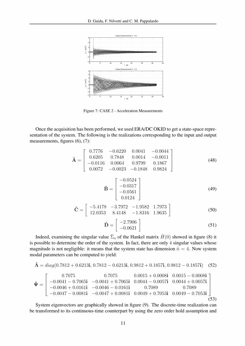
In the second case, we placed an additional mass on the first floor. In figure (6) is showedthe force measurement applied on the first floor and in figure (7) there is the system responsecorresponding to the input. Even in this case, in order to get statistically meaningful results, werepeated the experimental acquisition ten times but in the figures (6), (7) is showed only the firsttest.

0 5 10 15 20 25 30 35−0.5

0

0.5

1

1.5

2

t [s]

u [

N]

Generalized External Force N 1

Figure 6: CASE 2 - Force Measurement

10


0 5 10 15 20 25 30 35−4

−2

0

2

4

6

t [s]

y 1

[m

/s2 ]


0 5 10 15 20 25 30 35−3

−2

−1

0

1

2

3

4

t [s]

y 2

[m

/s2 ]


Figure 7: CASE 2 - Acceleration Measurements

Once the acquisition has been performed, we used ERA/DC OKID to get a state-space repre-sentation of the system. The following is the realizations corresponding to the input and outputmeasurements, figures (6), (7):

A =

0.7776 −0.6220 0.0041 −0.00440.6205 0.7848 0.0014 −0.0011−0.0116 0.0064 0.9799 0.18670.0072 −0.0023 −0.1848 0.9824

(48)

B =

−0.0524−0.0317−0.05610.0124

(49)

C =

[−5.4178 −3.7972 −1.9582 1.797312.0353 8.4148 −1.8316 1.9635

](50)

D =

[−2.7906−0.0621

](51)

Indeed, examining the singular value Σn of the Hankel matrix H(0) showed in figure (8) itis possible to determine the order of the system. In fact, there are only 4 singular values whosemagnitude is not negligible: it means that the system state has dimension n = 4. Now systemmodal parameters can be computed to yield:

Λ = diag(0.7812 + 0.6213i, 0.7812− 0.6213i, 0.9812 + 0.1857i, 0.9812− 0.1857i) (52)

Ψ =

0.7075 0.7075 0.0015 + 0.0008i 0.0015− 0.0008i

−0.0041− 0.7065i −0.0041 + 0.7065i 0.0044− 0.0057i 0.0044 + 0.0057i−0.0046 + 0.0161i −0.0046− 0.0161i 0.7089 0.7089−0.0047− 0.0081i −0.0047 + 0.0081i 0.0049 + 0.7053i 0.0049− 0.7053i

(53)

System eigenvectors are graphically showed in figure (9). The discrete-time realization canbe transformed to its continuous-time counterpart by using the zero order hold assumption and

11


0 10 20 30 40 50 60 70 80 90 10010

−16

10−14

10−12

10−10

10−8

10−6

10−4

10−2

100

102

104

Number

SV

Mag

nitu

de

Hankel Matrix Singular Values

Figure 8: CASE 2 - Hankel Matrix Singular Values

0 0.5 1 1.5 2 2.5 3−2.5

−2

−1.5

−1

−0.5

0

0.5

1

Degrees of Freedom

Mag

nitu

de


← Phase 0

← Phase −3.1521

0 0.5 1 1.5 2 2.5 30

0.2

0.4

0.6

0.8

1

Degrees of Freedom

Mag

nitu

de


← Phase 0 ← Phase −0.088383

Figure 9: CASE 2 - System Eigenvalues and Eigenvectors

subsequently modal damping rates and natural frequencies can be computed from the diagonalmatrix Λc ∈ Cn×n to yield:

fn,1 = 1.9056 [Hz] (54)

fn,2 = 6.8439 [Hz] (55)

ξ1 = 0.0075 [\] (56)

ξ2 = 0.0028 [\] (57)

Now it is straightforward to note that the effect of the additional mass is the reduction ofsystem natural frequencies whereas the damping ratios are roughly unaffected. At this point theoptimal damping coefficients α and β that fits in the least-square sense the identified naturalfrequencies can be computed according to equations (19) to yield:

α = 0.1752 (58)

β = 3.4355 · 10−5 (59)

12


This parameters have almost the same magnitude compared to the preceding case. Finally,using the MKR algorithm a mechanical model of system mass, stiffness and damping matricescan be computed to yield:

Φ =

[0.0168 + 0.0824i −0.0579− 0.1785i−0.0395− 0.1840i −0.0705− 0.1657i

](60)

M =

[1.3771 0.01190.0119 0.5566

][kg] (61)

K =

[630.44 −425.83−425.83 439.01

][kg/s2] (62)

R =

[59.9062 −34.1418−34.1418 38.4897

][kg/s] (63)

where Φ is system eigenvectors matrix scaled according to equations (28), (29). Even inthis case, while the identified mass M and stiffness K matrices are satisfactory acceptable, theidentified damping matrix R appears to be in some way incongruous. On the other hand, byusing the proposed formulae (19), the result is the following:

R =

[0.2739 −0.0223−0.0223 0.1231

][kg/s] (64)

this damping matrix is a better estimation of actual system damping. Note that there is amarked difference between results of case-study 1 and case-study 2. Indeed, the introduction ofthe additional mass on the first floor increases the magnitude of the first element of identifiedmass matrix M.

5 CONCLUSIONS

In this paper we performed an experimental investigation on a two-story frame in order toidentify a second-order mechanical model, that is to derive system mass, stiffness and dampingmatrices. First, we identified system modal parameters through Eigensystem Realization Al-gorithm with Data Correlation using Observer/Kalman Filter Identification (ERA/DC OKID)[4]. Then we obtained mass, stiffness and damping matrices using a numerical method (MKR)proposed by [5, 6, 7]. Authors also proposed a new method to identify damping matrix frommodal parameters [8, 9]. The structure was excited by an impulse yielded by 8202 Bruel &Kjaer impact hammer and the response was recorded by 4507 Bruel & Kjaer accelerometersconnected to 6160 Bruel & Kjaer Pulse spectrum analyzer. The identification procedure wascarried out several times, changing system mass and stiffness, and the results obtained are ingood agreement with our FEM simulations. This work is the first step of our research projectaimed at setting up a new virtual passive controller in order to regulate structural vibrations.

REFERENCES

[1] J. N. Juang, R. S. Pappa, An Eigensystem Realization Algorithm for Modal ParameterIdentification and Model Reduction. J. Guid. Control Dyn., 8(5), pp. 620627, 1985.

13


[2] J. N. Juang, J. E. Cooper, J. R. Wright, An Eigensystem Realization Algorithm Using DataCorrelation (ERA/DC) for Modal Parameter Identification. Cont. Theor. Adv. Technol.,4(1), pp. 514, 1988.

[3] J. N. Juang, M. Phan, L. G. Horta, R. W. Longman, Identification of Observer/KalmanFilter Markov Parameters: Theory and Experiments. J. Guid. Control Dyn., 16(2), pp.320329, 1993.

[4] J. N. Juang, Applied System Identification. Prentice Hall PTR, 1994.

[5] M. De Angelis, H. Lus, R. Betti, R. W. Longman, Extracting Physical Parameters ofMechanical Models from Identified State-Space Representations. J. App. Mech., 69, pp.617-625, 2002.

[6] H. Lus, M. De Angelis, R. Betti, R. W. Longman, Constructing Second-Order Models ofMechanical Systems from Identified State Space Realizations. Part I: Theoretical Discus-sions. J. Eng. Mech., 129(5), pp. 477-488, 2003.

[7] H. Lus, M. De Angelis, R. Betti, R. W. Longman, Constructing Second-Order Models ofMechanical Systems from Identified State Space Realizations. Part II: Numerical Investi-gations. J. Eng. Mech., 129(5), pp. 489-501, 2003.

[8] D. Guida, F. Nilvetti, C. M. Pappalardo, Parameter Identification of a Two Degrees ofFreedom Mechanical System. WSEAS transaction on International Journal of Mechanics(NAUN), 2(3), pp. 23-30, 2009.

[9] D. Guida, F. Nilvetti, C. M. Pappalardo, Parameter Identification of a Full-Car Model forActive Suspension. Worldwide Journal of Achievements in Materials and ManufacturingEngineering, 2(40), pp. 138-148, 2010.

14

Documents

MASS, STIFFNESS AND DAMPING IDENTIFICATION OF A …