LTE uplink scheduling inmulti-core systems

XINYUN LI

Master’s Degree ProjectStockholm, Sweden

XR-EE-LCN 2012:005

1

LTE uplink scheduling in multi core system

Xinyun Li

Examiner: Viktoria Fodor (KTH)

Supervisor: Carola Faronius (Ericsson)

Jon Sundberg (Ericsson)

Masters‟ Degree Project

Stockholm, Sweden 2011

2

Abbreviations ............................................................................................................................ 5

Table of Figures ......................................................................................................................... 6

Table of Tables .......................................................................................................................... 6

Abstract ..................................................................................................................................... 7

1 Introduction ....................................................................................................................... 8

1.1 Overview .................................................................................................................. 8

1.2 Objective and Limitations ........................................................................................ 8

1.3 Thesis Outline .......................................................................................................... 9

2 LTE Basics ...................................................................................................................... 11

2.1 Introduction ............................................................................................................ 11

2.2 LTE Time-Frequency Structure ............................................................................. 11

2.2.1 Uplink Modulation Reference Signals ............................................................... 12

2.2.2 Scheduling Element ........................................................................................... 12

2.2.3 LTE Frame Structure ......................................................................................... 13

2.2.4 LTE Bandwidth ................................................................................................. 13

2.3 Channel Dependent Scheduling ............................................................................. 13

2.4 LTE Uplink Scheduling ......................................................................................... 14

2.4.1 LTE Uplink Scheduling Procedure .................................................................... 14

2.4.2 Scheduling Request (SR) ................................................................................... 15

2.4.3 Scheduling Decision .......................................................................................... 15

Estimation Error .............................................................................................................. 16

2.4.4 Scheduling Grant ............................................................................................... 16

2.4.5 Buffer Status Report .......................................................................................... 16

2.5 Related Work ......................................................................................................... 16

3 Simulator ......................................................................................................................... 18

3.1 Simulator Overview ............................................................................................... 18

3.2 Channel Model ....................................................................................................... 19

3.3 Traffic Load ........................................................................................................... 20

4 Scheduler ......................................................................................................................... 21

3

4.1 Overview ................................................................................................................ 21

4.1.1 Number of DSPs ................................................................................................ 22

4.2 Pre-Scheduling Phase ............................................................................................. 23

4.2.1 Weight Calculation ............................................................................................ 24

4.3 Parallel Scheduling Phase ...................................................................................... 25

4.3.1 Throughput Calculation ..................................................................................... 26

4.4 Post-Scheduling Phase ........................................................................................... 26

5 Scheduling Algorithm ..................................................................................................... 28

5.1 Serial Scheduling ................................................................................................... 28

5.2 Pre-Scheduling Phase ............................................................................................. 28

5.2.1 Simple UE Division Scheme ............................................................................. 29

5.2.2 Advanced UE Division Scheme ........................................................................ 29

5.2.3 Simple Frequency Division Scheme .................................................................. 29

5.2.4 Advanced Frequency Division Scheme ............................................................. 30

5.3 Parallel Scheduling Phase ...................................................................................... 30

5.3.1 Maximum Throughput ....................................................................................... 30

5.3.2 Maximum Fairness ............................................................................................ 30

5.4 Post-Scheduling Phase ........................................................................................... 30

5.4.1 Simple Post-Scheduling Phase........................................................................... 31

5.4.2 Advanced Post-Scheduling Phase ...................................................................... 31

6 Performance Evaluation .................................................................................................. 32

6.1 Simulation Scenarios .............................................................................................. 32

6.1.1 Simulation 1 ....................................................................................................... 32

6.1.2 Simulation 2 ....................................................................................................... 32

6.1.3 Simulation 3 ....................................................................................................... 32

6.1.4 Simulation 4 ....................................................................................................... 33

6.2 Results .................................................................................................................... 33

6.2.1 Reference Simulation ......................................................................................... 34

6.2.2 Simulation 1 ....................................................................................................... 35

6.2.3 Simulation 2 ....................................................................................................... 39

4

6.2.4 Simulation 3 ....................................................................................................... 41

6.2.5 Simulation 4 ....................................................................................................... 46

7 Discussions ...................................................................................................................... 49

7.1 Conclusion ............................................................................................................. 49

7.2 Future Work ........................................................................................................... 50

8 References ....................................................................................................................... 52

5

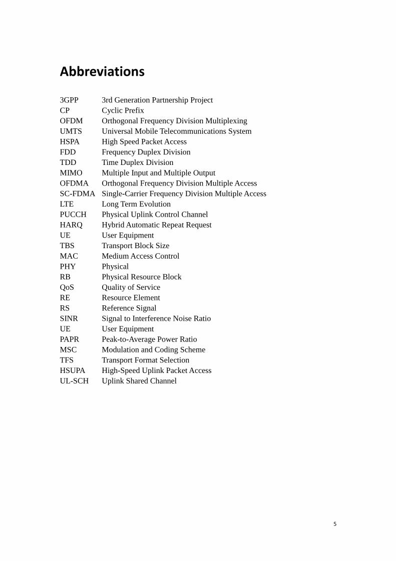
Abbreviations

3GPP 3rd Generation Partnership Project

CP Cyclic Prefix

OFDM Orthogonal Frequency Division Multiplexing

UMTS Universal Mobile Telecommunications System

HSPA High Speed Packet Access

FDD Frequency Duplex Division

TDD Time Duplex Division

MIMO Multiple Input and Multiple Output

OFDMA Orthogonal Frequency Division Multiple Access

SC-FDMA Single-Carrier Frequency Division Multiple Access

LTE Long Term Evolution

PUCCH Physical Uplink Control Channel

HARQ Hybrid Automatic Repeat Request

UE User Equipment

TBS Transport Block Size

MAC Medium Access Control

PHY Physical

RB Physical Resource Block

QoS Quality of Service

RE Resource Element

RS Reference Signal

SINR Signal to Interference Noise Ratio

UE User Equipment

PAPR Peak-to-Average Power Ratio

MSC Modulation and Coding Scheme

TFS Transport Format Selection

HSUPA High-Speed Uplink Packet Access

UL-SCH Uplink Shared Channel

6

Table of Figures

Figure 1 Resource Grid for one Scheduling Resource Block ................................... 12

Figure 2 LTE Frame Structure .................................................................................. 13

Figure 3 eNodeB and User Equipment Interaction ................................................... 15

Figure 4 Cumulative Distribution Function of SINR Values ................................... 19

Figure 5 Channel Condition with Rayleigh Fading .................................................. 20

Figure 6 Parallel Scheduling Algorithm Structure .................................................... 22

Figure 7 Theoretical Scheduling Delay Weight Form .............................................. 25

Figure 8 Pre-Scheduling Phase Structure ................................................................. 29

Figure 9 Throughput trend with different NrOfDSPs ............................................... 36

Figure 10 Time Consumption for different Phases ................................................... 36

Figure 11 Total Time Consumption for Scheduling Processes ................................ 37

Figure 12 Throughput Performance at Scheduling Phases ....................................... 39

Figure 13 Time Consumption at Scheduling Phases ................................................ 40

Figure 14 Average Scheduled Number of UE .......................................................... 41

Figure 15 Average Scheduled Number of UE .......................................................... 42

Figure 16 Number of RBs per Scheduled UE ........................................................... 43

Figure 17 Throughput per Scheduled UE ................................................................. 44

Figure 18 Data Rate per Scheduled RB .................................................................... 45

Figure 19 Throughput trend with different Scheduling Phases ................................ 46

Figure 20 Time Consumption in different Scheduling Phases ................................. 47

Figure 21 Throughput/Time Efficiency .................................................................... 48

Table of Tables

Table 1 Different Number of RBs for different LTE bandwidth .............................. 13

Table 2 MCS Switching Threshold and Derived Spectral Efficiency ...................... 26

Table 3 Bits/symbol Rate with Different Modulation Scheme ................................. 26

Table 4 Setting for Simulation 1 ............................................................................... 32

Table 5 Setting for Simulation 2 ............................................................................... 32

Table 6 Setting for Simulation 3 ............................................................................... 33

Table 7 Setting for Simulation 4 ............................................................................... 33

Table 8 Maximizing Throughput .............................................................................. 34

Table 9 Maximizing Fairness .................................................................................... 35

7

Abstract

With the goal to achieve higher and higher performance with the next-generation of

Long Term Evolution (LTE) equipment, multi-core processors are implemented more

and more inside LTE eNodeB. The development and increasing use of multi-core

processors system raises a challenge to the current scheduling algorithm. The intuitive

way of scheduling is a serial process, by which users are scheduled one after another

within one cell. It becomes very inefficient in a multi core system, since the

parallelism provided by the multi core platform is not fully utilised.

The goal of this study is to investigate how the uplink scheduler algorithm can be

parallelised efficiently over several DSPs in a multi-core environment. In this thesis, a

three-phase algorithm is presented. For each phase, two solutions are provided and

evaluated against each other in terms of throughput, time efficiency and fairness, the

result is compared with serial scheduling process.

The simulation result indicates that the parallel scheduling algorithm is able to

achieve higher time efficiency than serial scheduling algorithm, while keeping the

same throughput performance. The time improvement depends on the number of

schedulable UEs in the system, processors number, the solution used in each phase

and the throughput trade-off.

8

1 Introduction

In this section, an overview introduction of the thesis background, aim and motivation

will be presented. A short thesis outline of this report will also be given in the end.

1.1 Overview

This master thesis is performed in Ericsson Design & System, focusing on the LTE

uplink scheduling algorithm investigation. The main objective of the thesis work is to

design a parallel processing algorithm for LTE uplink in a multi processor system and

evaluate the performance of this algorithm with respect to throughput, efficiency as

well as algorithm complexity.

With the goal to achieve higher and higher performance for the next-generation of

Long Term Evolution (LTE) equipment, multi-core processors which cram multiple

microprocessors onto one chip, will be implemented more and more inside LTE

eNodeB. However, the development and increasing use of multi-core processors

system raises a challenge to the current scheduling algorithm on the singular

processor platform. Since the intuitive way of scheduling is, to be simple, a serial

process. After prioritizing the schedulable users in one scheduling time unit, the

scheduler assigns resources to these users according to the priority level one by one

until there are no more users to be scheduled or there is no spectral resource left

according to the scheduling algorithm.

While this scheduling algorithm works fine in single DSP platform, it becomes very

inefficient on a multi-core platform. The reason is, during the resource allocation

processes, low priority user equipment can not be scheduled until the former users get

scheduled. However, in a multi-core environment the parallelism provided by this

platform is wasted in this serial way of scheduling, only one processor is working on

scheduling process even when there are other free processors ready to provide service.

Since the available time for the scheduling process is strictly limited, it directly

restricts the number of user equipments that can transmit in one time unit. If the

multi-processor system provides the possibility to run scheduling process in parallel,

more user equipments can be allocated into spectrum by increasing the number of

processors number. The proposal of parallel scheduling can be a promising way to

increase current system performance and it is the main topic investigated in this

master thesis.

1.2 Objective and Limitations

The target of this thesis is to investigate, on a system level first, how the uplink

scheduler process can be parallelised efficiently over several DSPs in a multi-core

environment, i.e to divide the scheduling execution on multiple DSP-cores. By

dividing UEs into separated user groups, each UE group is granted with one processor.

9

The frequency resource is also divided into separated fragments, and then mapped to

different UE groups. The multi processors run the scheduling process independently

from each other. One processor is responsible for only part of the total UE population,

and has access only to part of the frequency resources. The reduced number of users

may result in decreasing of scheduling time, thus it is possible to schedule more users

within the same span of time. However, the parallel scheduling method may also

cause decrease of the system throughput as a side effect.

Since the available frequency resources are divided into several fragments and

matching each to a certain UE group, the user equipments in one group can move

around only within this fragment. They are not allowed to go over fragment boundary

and get allocated in other part of spectrum. Thus, compared with serial scheduling,

parallel algorithm may cause users to settle in worse frequency resources.

This study is to investigate how the uplink scheduler algorithm can be parallelised

efficiently over several DSPs both from time and throughput perspective. The

following paragraph gives a general introduction of the algorithm and its evaluation

process.

The algorithm presented in this paper can be divided into three phase. In the first

phase, the pre-scheduling phase, user equipments and frequency band is divided into

Groups and Fragments according to different rules, and each group is matched with

one fragment. In the second phase, the parallel scheduling phase, the multi processors

platform takes over the scheduling process by running spectrum allocation in parallel

streams. In this phase, two methods are designed and evaluated in our study:

throughput maximizing and fairness maximizing. In the last phase, which is called

post scheduling phase, the main purpose is taking advantage of the time saved by

Phase 2 to improve spectral efficiency.

For each phase, two solutions are provided and evaluated against each other in terms

of throughput, time efficiency and fairness. The proposed algorithm is also evaluated

against serial scheduling algorithm with respect to throughput, time efficiency,

memory usage, and implementation possibility.

Considering limitation of the scope of this thesis, the simulation is implemented

without memory from different scheduling processes, which means there is no

interaction between previous time units with the next one. Since the diversity of

performed simulations are based on variation of scheduling algorithm, this thesis will

not delve deep in how different traffic loads and channel models affect the

performance of the scheduling process.

1.3 Thesis Outline

The thesis report starts with a background introduction in Chapter 1. Chapter 2 is

designed to explain the LTE basics knowledge related to this thesis topic. Chapter 3

gives a detailed introduction of the current simulation environment used in this thesis.

The scheduler structure is described in a separated chapter in Chapter 4, followed by

Chapter 5, which introduces four simulation cases. The report ends with the result

presentations and conclusion in Chapter 6 and 7.

10

11

2 LTE Basics

2.1 Introduction

3GPP Long Term Evolution (LTE), introduced in 3GPP Release 8, is a standard for

wireless communication of high-speed data. It introduces a flat, all IP-based network

architecture, which represents a significant change to the 3G UMTS/HSPA radio

access and core networks. A common, packet-based infrastructure is used for all

services (voice and data), removing the need for the dedicated circuit-switched and

packet-switched domains which are present in 3G UMTS/HSPA networks. The radio

access network is simplified in LTE with the base station, or evolved-NodeB

(eNodeB), implementing the functions which were previously distributed between the

3G RNC and NodeB. [1]

As a data dominated network, LTE is focusing on supporting Packet-Switched (PS)

Service. The performance of LTE system shall fulfil a number of requirements

regarding throughput and latency. Significantly increased peak data rate should be

delivered and improved spectrum efficiency should be achieved in LTE system. Some

details can be summarized as follows: [1]

- Data Rate: Peak data rates target 100 Mbps (downlink) and 50 Mbps (uplink) for 20

MHz spectrum allocation, with a 2-by-2 Multiple Input and Multiple Output (MIMO)

transmission system, while 2 receive antennas are available at UE and 2 transmit

antenna at the base station.

- Spectrum Efficiency: Downlink target is 3-4 times better than release 6 High-Speed

Uplink Packet Access (HSUPA), uplink target for 2-3 times better than release 6

HSUPA.

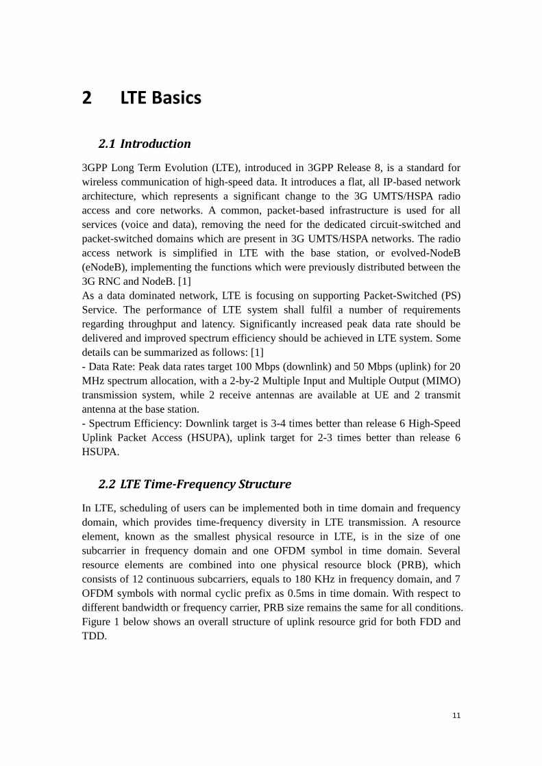
2.2 LTE Time-Frequency Structure

In LTE, scheduling of users can be implemented both in time domain and frequency

domain, which provides time-frequency diversity in LTE transmission. A resource

element, known as the smallest physical resource in LTE, is in the size of one

subcarrier in frequency domain and one OFDM symbol in time domain. Several

resource elements are combined into one physical resource block (PRB), which

consists of 12 continuous subcarriers, equals to 180 KHz in frequency domain, and 7

OFDM symbols with normal cyclic prefix as 0.5ms in time domain. With respect to

different bandwidth or frequency carrier, PRB size remains the same for all conditions.

Figure 1 below shows an overall structure of uplink resource grid for both FDD and

TDD.

12

Figure 1 Resource Grid for one Scheduling Resource Block

2.2.1 Uplink Modulation Reference Signals

Within the resource block structure, uplink demodulation reference signals are located

at the forth symbol of each uplink slot. For every sub-frame, there are two reference

signal transmissions, one in each slot.

Uplink modulation reference signals are used for channel estimation for coherent

demodulation of the Physical Uplink Shared Channel (PDCCH) and Physical Uplink

Control Channel (PUCCH). Thus, they are transmitted with PUSCH or PUCCH with

the same bandwidth as the corresponding physical channel. [12]

2.2.2 Scheduling Element

From scheduling perspective, the smallest scheduling unit is a scheduling resource

block, which is 180 KHz in frequency domain, and 1ms in time domain. One

Scheduling Resource Block (SRB) equals to the size of two Physical Resource Blocks

(PRS) in time domain.

To simplify, in this report, we use resource block (RB) to refer to scheduling resource

block (SRB). But just to be clear, scheduling block and physical resource block is two

Resource Block

(12 subcarriers in

frequency, one slot

in time domain)

One slot

One subframe = 1ms

One Resource

Element

OFDM Symbols (Normal Cyclic Prefix)

Subcarrie

rs

13

different structures and with different size in time domain.

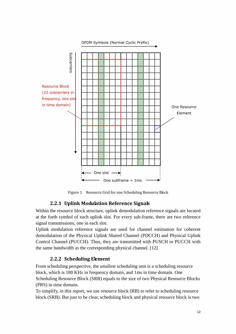
2.2.3 LTE Frame Structure

In time domain, one Transmission Time Interval (TTI) has the same length as one

sub-frame in LTE system. Taking FFD model as example, the general frame length in

time domain lasts 10 ms, which can be divided into 20 slots, each slot has a duration

of 0.5 ms. One LTE sub frame consists two slots which equals to 1 ms in total. [5]

Figure 2 LTE Frame Structure

2.2.4 LTE Bandwidth

In frequency domain, LTE supports a high degree of bandwidth flexibility, allowing

for a an overall transmission bandwidth ranging from 1.4MHz up to 20MHz, which

corresponds to 6 to 100 RBs.

The numbers of RBs with respect to different bandwidth is shown in the following

table. [4]

Table 1 Different Number of RBs for different LTE bandwidth

Channel Bandwidth 1.4 3 5 10 15 20

Number of Resource Blocks 6 15 25 50 75 100

2.3 Channel Dependent Scheduling

The purpose of scheduling is to decide which terminal will transmit data on which set

of resource blocks with what transport format to use. The objective is to assign

resources to the terminal such that the quality of service (QoS) requirement is fulfilled.

Scheduling decision is taken every 1 ms by base station (termed as eNodeB) as the

same length of Transmission Time Interval (TTI) in LTE system.

In general, two types of scheduling can be implemented in uplink scheduler, channel

dependent scheduling and non channel dependent scheduling.

Non channel dependent scheduling does not consider channel condition during a

scheduling process. The users without channel quality information can obtain

Subframe 0 Subframe 1 Subframe 2 Subframe 3 Subframe 4

One Radio Frame T=10ms

One Slot T = 0.5 ms

One Subframe T = 1 ms

One half Frame 5ms

14

frequency diversity gain through frequency hopping, and the system capacity can be

improved without increasing equipment costs. [1]

Channel dependent scheduling takes into account of the channel variations between

mobile terminals and base station. Since channel condition is time-varying due to

fading and shadowing, different user terminals experience different channel condition

at a given time. At one specific time slot, there is a high possibility some users are

experiencing good channel conditions. By allowing these user terminals to transmit,

the spectrum is used in an efficient way and the total throughput of the system will be

maximized. [11][12] With channel dependent scheduling algorithm, user equipments

are granted with the advantageous frequency resources which provide better channel

condition within the total frequency band. The time-frequency scheduling structure

provides the diversity for users to choose the scheduling elements in both domains. If

the scheduling resources are in favorable conditions and user service requirement is

flexible, the spectrum utilization and system throughput will be improved.

However, compared with non channel dependent scheduling, the performance

increase comes at the cost of complexity of the system.

On the other hand, channel dependent scheduling can give raise to fairness problem.

Since channel dependent scheduling algorithm grants users with better channel

performance higher priority to transmit, during one sub-frame, the bad performed

users may be starved for their low Signal-to-noise-and-interference ratio (SINR) level.

From mobility perspective, fast moving users may get out of fading with a higher

speed, but in reality, the users in slow fading or located at the edge of cell suffer from

bad channel condition for a significant amount of time. In these cases, the scheduling

algorithm put these users at a risk of never getting scheduled if the channel condition

varies slowly.[1]

Thus, when designing a scheduling algorithm, issues above need to be considered. A

compromised solution needs to be made between wireless resource efficiency and

levels of fairness among users.

2.4 LTE Uplink Scheduling

In LTE uplink Single-carrier Frequency Division Multiple Access (SC-FDMA) is

implemented to provide orthogonality between different users and remain at a low

peak-to-average power ratio (PAPR) level. [10] However, unlike OFDMA, user

equipments transmitted in SC-FDMA scheme are only allowed to take continuous

frequency recourses. Thus during scheduling, each user is constrained to use

consecutive resource blocks.[18]

2.4.1 LTE Uplink Scheduling Procedure

At the beginning of scheduling process, the buffer sizes of UEs are not available to

uplink scheduler. After some initial setup signaling, user equipment sends a

scheduling request (SR) to notify base station that this UE has data to transmit. The

SR does not contain buffer status information, and then scheduler assigns initial

resources without detailed knowledge of buffer content. In order to require the buffer

15

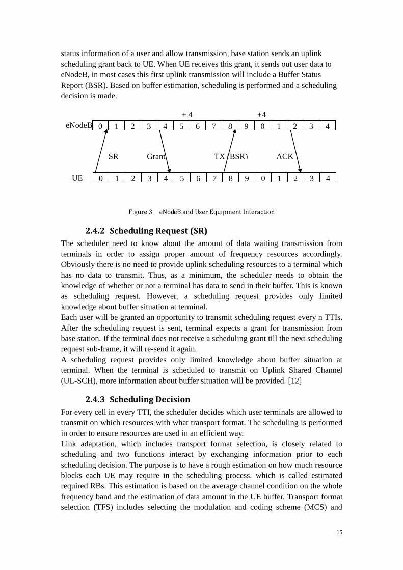
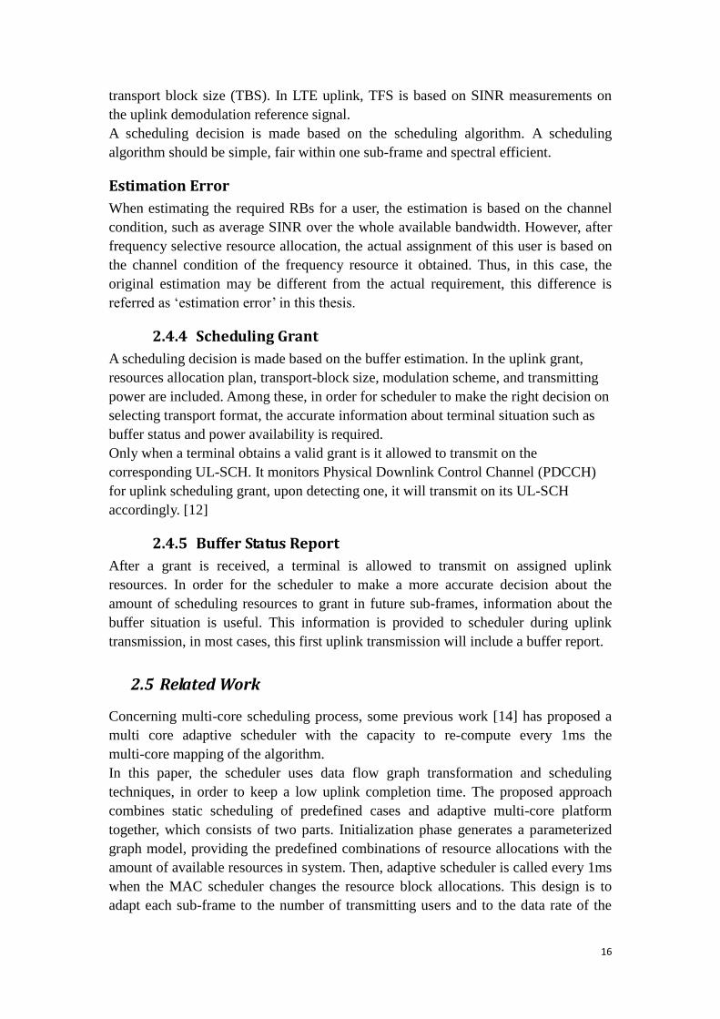
status information of a user and allow transmission, base station sends an uplink

scheduling grant back to UE. When UE receives this grant, it sends out user data to

eNodeB, in most cases this first uplink transmission will include a Buffer Status

Report (BSR). Based on buffer estimation, scheduling is performed and a scheduling

decision is made.

Figure 3 eNodeB and User Equipment Interaction

2.4.2 Scheduling Request (SR)

The scheduler need to know about the amount of data waiting transmission from

terminals in order to assign proper amount of frequency resources accordingly.

Obviously there is no need to provide uplink scheduling resources to a terminal which

has no data to transmit. Thus, as a minimum, the scheduler needs to obtain the

knowledge of whether or not a terminal has data to send in their buffer. This is known

as scheduling request. However, a scheduling request provides only limited

knowledge about buffer situation at terminal.

Each user will be granted an opportunity to transmit scheduling request every n TTIs.

After the scheduling request is sent, terminal expects a grant for transmission from

base station. If the terminal does not receive a scheduling grant till the next scheduling

request sub-frame, it will re-send it again.

A scheduling request provides only limited knowledge about buffer situation at

terminal. When the terminal is scheduled to transmit on Uplink Shared Channel

(UL-SCH), more information about buffer situation will be provided. [12]

2.4.3 Scheduling Decision

For every cell in every TTI, the scheduler decides which user terminals are allowed to

transmit on which resources with what transport format. The scheduling is performed

in order to ensure resources are used in an efficient way.

Link adaptation, which includes transport format selection, is closely related to

scheduling and two functions interact by exchanging information prior to each

scheduling decision. The purpose is to have a rough estimation on how much resource

blocks each UE may require in the scheduling process, which is called estimated

required RBs. This estimation is based on the average channel condition on the whole

frequency band and the estimation of data amount in the UE buffer. Transport format

selection (TFS) includes selecting the modulation and coding scheme (MCS) and

0 1 2 3 4 5 6 7 8 9 0 1 2 3 4

SR Grant TX (BSR) ACK

UE 0 1 2 3 4 5 6 7 8 9 0 1 2 3 4

eNodeB

+ 4 +4

16

transport block size (TBS). In LTE uplink, TFS is based on SINR measurements on

the uplink demodulation reference signal.

A scheduling decision is made based on the scheduling algorithm. A scheduling

algorithm should be simple, fair within one sub-frame and spectral efficient.

Estimation Error

When estimating the required RBs for a user, the estimation is based on the channel

condition, such as average SINR over the whole available bandwidth. However, after

frequency selective resource allocation, the actual assignment of this user is based on

the channel condition of the frequency resource it obtained. Thus, in this case, the

original estimation may be different from the actual requirement, this difference is

referred as „estimation error‟ in this thesis.

2.4.4 Scheduling Grant

A scheduling decision is made based on the buffer estimation. In the uplink grant,

resources allocation plan, transport-block size, modulation scheme, and transmitting

power are included. Among these, in order for scheduler to make the right decision on

selecting transport format, the accurate information about terminal situation such as

buffer status and power availability is required.

Only when a terminal obtains a valid grant is it allowed to transmit on the

corresponding UL-SCH. It monitors Physical Downlink Control Channel (PDCCH)

for uplink scheduling grant, upon detecting one, it will transmit on its UL-SCH

accordingly. [12]

2.4.5 Buffer Status Report

After a grant is received, a terminal is allowed to transmit on assigned uplink

resources. In order for the scheduler to make a more accurate decision about the

amount of scheduling resources to grant in future sub-frames, information about the

buffer situation is useful. This information is provided to scheduler during uplink

transmission, in most cases, this first uplink transmission will include a buffer report.

2.5 Related Work

Concerning multi-core scheduling process, some previous work [14] has proposed a

multi core adaptive scheduler with the capacity to re-compute every 1ms the

multi-core mapping of the algorithm.

In this paper, the scheduler uses data flow graph transformation and scheduling

techniques, in order to keep a low uplink completion time. The proposed approach

combines static scheduling of predefined cases and adaptive multi-core platform

together, which consists of two parts. Initialization phase generates a parameterized

graph model, providing the predefined combinations of resource allocations with the

amount of available resources in system. Then, adaptive scheduler is called every 1ms

when the MAC scheduler changes the resource block allocations. This design is to

adapt each sub-frame to the number of transmitting users and to the data rate of the

17

services they require.

Although the scheduling method in this paper opens a creative way of scheduling for

LTE uplink, the proposed scheduling requirements such as memory requirement and

the adaptive multi-core system are not implementable in our system.

Some previous work [13] has focus on opportunistic scheduling algorithm. A solution

called Heuristic Localized Gradient Algorithm (HLGA) is used for uplink scheduling

in 3G LTE system. It allows the users maximize a certain criteria to be scheduled first,

and the rest left resources are divided to other users. The algorithm is mainly

structured from a gradient algorithm for the scheduling but adopts a heuristic

approach in the allocations of the scheduled bands. Gradient based algorithm means,

select the transmission rate vector that maximizes the projection onto the gradient of

the system‟s total utility. [21] In this paper, a procedure named „pruning‟ is presented.

Resources blocks are assigned to users by HLGA regardless of the amount of data

they have in the buffer. After resource allocation, pruning is implemented to search for

free RBs that can be allocated to other unsatisfied users.

This pruning procedure serves similar function as Phase 3 in our scheduling algorithm,

and it is based on the estimation error we described in previous sections. However,

this scheduling algorithm presented in this report is theoretical optimum scheduling

process. The time to implement pruning is strictly limited by the number of users in

the system, and HLGA solution for resource allocation has high demand on memory

resources and processing ability. Thus in our report, by paralleling the scheduling

process, we try to gain more time for later improvement such as implementing

pruning.

18

3 Simulator

Since the conclusion of this thesis is mostly based on simulation result, the simulation

settings will directly affect the performance that is derived. This section will be

contributed to simulator structure and settings descriptions. However, the scheduler

structure will be presented in a separated chapter in Chapter 4 .

This chapter starts with a general introduction of the simplified system model we used,

which followed by an overall picture of the simulator structure. The settings and

limitations of this simulation environment will be explained in the next two sections.

3.1 Simulator Overview

The main aim of this thesis is to compare algorithm performance between the serial

and paralleled way of scheduling, at the same time for parallel scheduling algorithm,

performance differences between solutions in each phase are also investigated. The

variety of performed simulations is mostly based on changes in scheduling algorithm.

Thus, we provide only one setting for the simulation environment to reduce the

complexity.

The simulation environment we built in Matlab works TTI independently. For each

time unit it generates a whole new set of user data and channel condition randomly

according to simulation setting. Data during the scheduling process, such as spectrum

allocation, throughput performance and time consumption are recorded for later

analysis. However, this information is not taken into account during next scheduling

process in the following time unit.

The simulator in Matlab can generate accurate result for throughput performance

based on the simulation settings, but the time consumption generated by Matlab is

based on the time cost for Matlab to run the scheduling process. This time

consumption does not take hardware limitation into account, such as the time needed

for loading data to local DSP memory and the time required for saving it. But this

result reflects the complexity of solutions differences between different scheduling

solutions, and it is enough for comparing solution. The throughput-time trade-off and

all the time-related results in this report are based on this assumption.

The time estimation in hardware scheduling environment is further investigated later

in this thesis. The estimation is based on the result from simulation environment of the

current implementation. The clock cycle generated by this simulation environment is

exactly the same as hardware generation. By dividing the designed scheduling

algorithm into smaller functions and comparing them with the functions we have in

the current system, estimated time consumption is derived. However, due to

confidentiality, the result and analysis will not be presented in this thesis report.

19

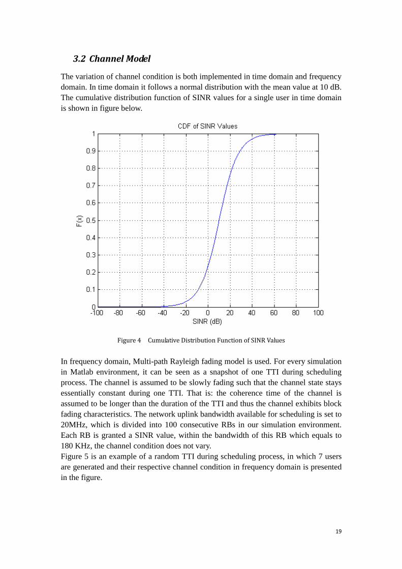
3.2 Channel Model

The variation of channel condition is both implemented in time domain and frequency

domain. In time domain it follows a normal distribution with the mean value at 10 dB.

The cumulative distribution function of SINR values for a single user in time domain

is shown in figure below.

Figure 4 Cumulative Distribution Function of SINR Values

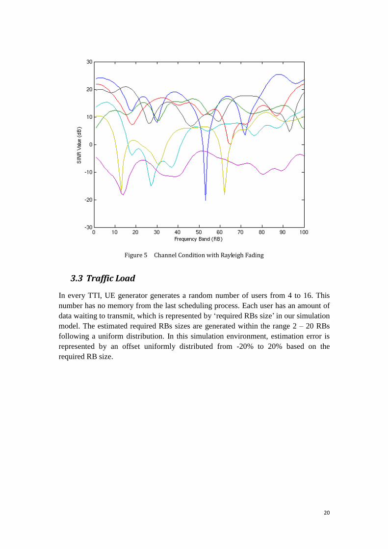
In frequency domain, Multi-path Rayleigh fading model is used. For every simulation

in Matlab environment, it can be seen as a snapshot of one TTI during scheduling

process. The channel is assumed to be slowly fading such that the channel state stays

essentially constant during one TTI. That is: the coherence time of the channel is

assumed to be longer than the duration of the TTI and thus the channel exhibits block

fading characteristics. The network uplink bandwidth available for scheduling is set to

20MHz, which is divided into 100 consecutive RBs in our simulation environment.

Each RB is granted a SINR value, within the bandwidth of this RB which equals to

180 KHz, the channel condition does not vary.

Figure 5 is an example of a random TTI during scheduling process, in which 7 users

are generated and their respective channel condition in frequency domain is presented

in the figure.

20

Figure 5 Channel Condition with Rayleigh Fading

3.3 Traffic Load

In every TTI, UE generator generates a random number of users from 4 to 16. This

number has no memory from the last scheduling process. Each user has an amount of

data waiting to transmit, which is represented by „required RBs size‟ in our simulation

model. The estimated required RBs sizes are generated within the range 2 – 20 RBs

following a uniform distribution. In this simulation environment, estimation error is

represented by an offset uniformly distributed from -20% to 20% based on the

required RB size.

21

4 Scheduler

In the previous chapter, we gave an overall picture of the simulator and the

description of simulation settings. Since the scheduling algorithm has a three-phase

structure, the settings and functions of the scheduler will be explained phase by phase.

Due to confidentiality, the detailed scheduling algorithm will not be described, but in

the next chapter the scheduling solutions in each phase will be presented at a general

level.

This chapter starts by giving an overview picture of the scheduler simulation scenario.

It follows by descriptions of the three-phase structure used for scheduler in this thesis.

In each phase, the limitations and important factors which may affect the scheduling

result are discussed.

4.1 Overview

In this thesis, most of the focus is put on the scheduler algorithm design and

performance evaluation. The scheduling algorithm in this thesis has three phases, in

each phase two solutions are designed for comparison. The scheduler gets UE list,

channel condition together with the available frequency resource as input. After

scheduling, the spectrum efficiency and time consumption of scheduling process are

evaluated with respect to different solutions.

As stated in the former chapters, compared with serial scheduling, the paralleled

scheduling has a risk of decreasing spectral efficiency performance. In order to reduce

this degradation, scheduling algorithm needs to be improved. On the other hand, even

though an algorithm can generate good throughput result, the complexity may also

stop it being implemented in hardware environment. Thus, both throughput

performance and complexity need to be considered when designing a scheduling

algorithm.

In this thesis, a three phase scheduling structure is chosen to be studied. The process

begins with Pre-scheduling Phase, which can also be seen as scheduling preparation

phase, the user equipments are divided into Groups and frequency resource is divided

into Fragment. The order of UEs getting scheduled and which frequency fragment

users would get are also planed in this phase. Based on the priority of users decided in

Phase 1, the UE goes through the second phase, which is parallel scheduling phase.

According to the chosen solution in this phase, UEs will be allocated one by one in

the assigned frequency fragment. Different groups of UEs are processed by different

processors in parallel, thus there is no interaction between different processor and UE

groups. The parallelism provided by the multi-core platform is used to provide the

possibility of scheduling more users or to save clock cycles. At the end of scheduling

process, Post-scheduling Phase is introduced, which is the last chance in this

scheduling process to improve the spectrum efficiency. In the last phase, different

solutions are used to increase throughput, which include extending the current

22

resource allocation and reallocating the users, more details will be shown in next

chapter.

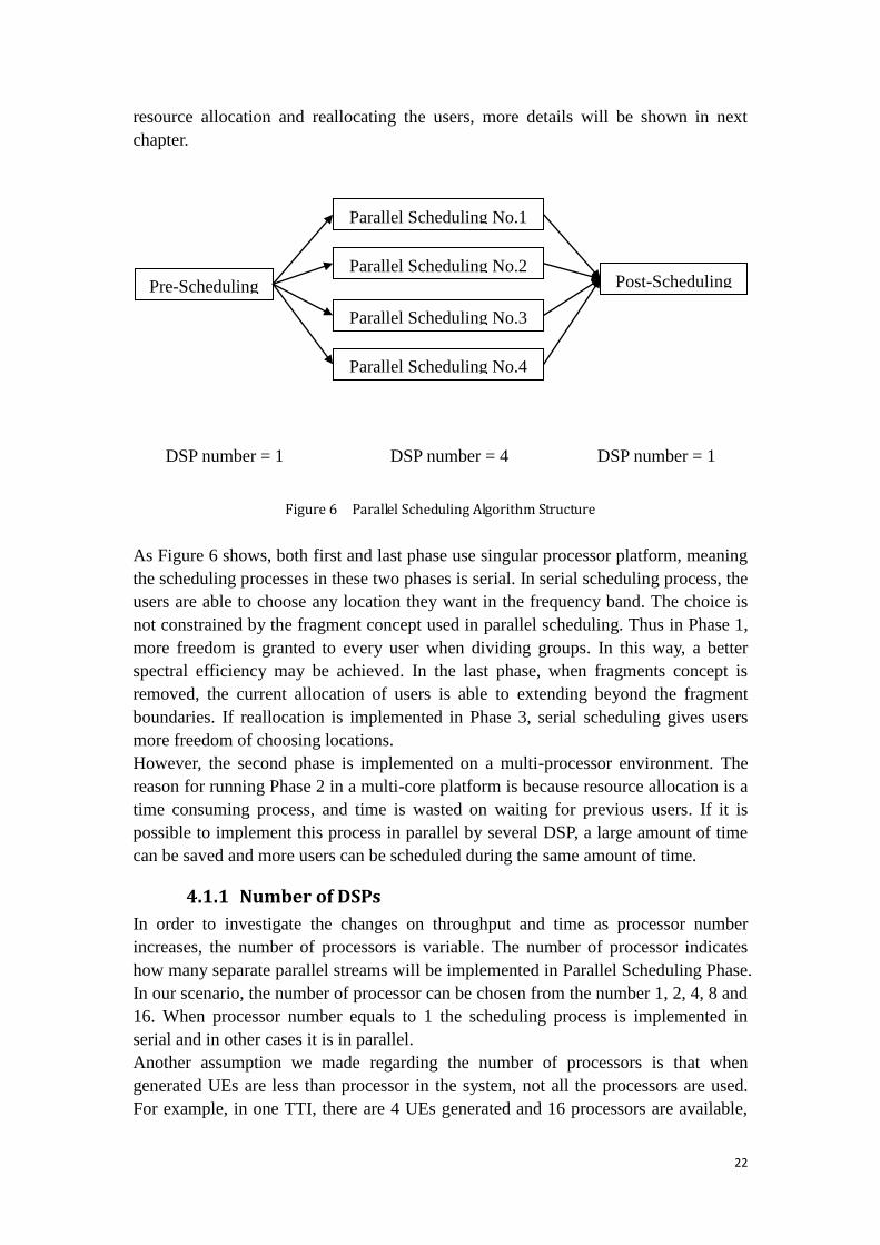
Figure 6 Parallel Scheduling Algorithm Structure

As Figure 6 shows, both first and last phase use singular processor platform, meaning

the scheduling processes in these two phases is serial. In serial scheduling process, the

users are able to choose any location they want in the frequency band. The choice is

not constrained by the fragment concept used in parallel scheduling. Thus in Phase 1,

more freedom is granted to every user when dividing groups. In this way, a better

spectral efficiency may be achieved. In the last phase, when fragments concept is

removed, the current allocation of users is able to extending beyond the fragment

boundaries. If reallocation is implemented in Phase 3, serial scheduling gives users

more freedom of choosing locations.

However, the second phase is implemented on a multi-processor environment. The

reason for running Phase 2 in a multi-core platform is because resource allocation is a

time consuming process, and time is wasted on waiting for previous users. If it is

possible to implement this process in parallel by several DSP, a large amount of time

can be saved and more users can be scheduled during the same amount of time.

4.1.1 Number of DSPs

In order to investigate the changes on throughput and time as processor number

increases, the number of processors is variable. The number of processor indicates

how many separate parallel streams will be implemented in Parallel Scheduling Phase.

In our scenario, the number of processor can be chosen from the number 1, 2, 4, 8 and

16. When processor number equals to 1 the scheduling process is implemented in

serial and in other cases it is in parallel.

Another assumption we made regarding the number of processors is that when

generated UEs are less than processor in the system, not all the processors are used.

For example, in one TTI, there are 4 UEs generated and 16 processors are available,

Parallel Scheduling No.1

Post-Scheduling Parallel Scheduling No.2

Parallel Scheduling No.3

Parallel Scheduling No.4

DSP number = 1 DSP number = 4 DSP number = 1

Pre-Scheduling

23

then only 4 processors are used out of the 16.

4.2 Pre-Scheduling Phase

As the first scheduling phase, pre-scheduling phase serves as a preparation function in

the whole scheduling process. The main purpose of this phase can be separated into

two parts.

The first one is dividing available frequency band in the system into N Fragments, and

N here equals to the number of processors according to our simulation setting.

The second function is dividing UEs into Groups as the same. For parallel scheduling

in the next phase, each processor is responsible for one group. When dividing UEs

into groups, in order to achieve a higher spectral efficiency and time efficiency at the

end of scheduling process, several conditions need to be taken into consideration, the

details will be explained below.

First, we consider time efficiency. When processing in parallel, one processor is

responsible for one group, but the whole resource allocation process ends only when

all the processors finish their works. In this case, the most efficient way to allocate

resource is when every processor finishes at the same time, i.e. every DSP gets a UE

group with the same size. The „size‟ here can be interpreted in many ways, depending

on what is the key factor affecting processing time, for example the estimated

required RBs in one UE group, or the number of users in each group. In hardware

environment, the loading time and memory usage may also affect the processing time,

but in our simulation assumption, these factors are not considered. Thus, to simplify,

in this simulation the meaning of „size‟ is narrowed down to the “required RB size” in

each UE group. By having the similar group sizes, different processors require similar

time for resource allocation, meaning no processor would waste time waiting for other

processors during parallel scheduling phase.

Apart from time efficiency, a good pre-scheduling solution should also target for

higher spectral efficiency. As is explained before, parallel scheduling generally

reduces the time cost for resource allocation process, however may decrease the

spectral efficiency at the same time. Although the decrease of throughput is

theoretically inevitable, a well-designed pre-scheduling solution may reduce the

degradation to a minimal level.

In order to achieve a high throughput, the most straight forward method would be

giving each UE the fragment with best channel condition. How to calculate the best

fragment for one user is the first step deciding UE groups. However, in practical

implementation, how to evaluate the channel condition in one fragment when it varies

in frequency domain is a tricky topic. For example, a fragment may have one RB with

high SINR value but decrease fast in the adjacent RBs. In another case, it may be in

good channel condition in general but dragged down by a few „bad‟ RBs. Both peak

and average value are not 100 percent reliable or fair to evaluate channel condition,

but taken all these factors into consideration, the calculation itself is also a

compromise of accuracy and complexity. A solution that can reach a balanced

between the two factors is good enough.

24

On the other hand, even the best fragment can be accurately decided, whether the user

can be allocated accordingly also depends on its scheduling priority in its group. As

was discussed in the first chapter, within one UE group lower priority users are

scheduled after high priority users. There is a possibility one UE will not get its best

RBs because they are already taken by previously scheduled UEs. Since the order of

user getting scheduled has a large impact on the final scheduling result, each user is

granted a weight deciding its scheduling priority. More details about the weight

system are introduced below.

4.2.1 Weight Calculation

Weight system is used for deciding the order of UEs to be divided into group. For

each UE, the higher the weight is, the earlier it can choose the group. At the same time,

the scheduling order of UE in each group is also decided at this moment.

Channel-Dependent Weight

When link adaptation is used in the system, it would be resource consuming to

transmit a certain amount of data to a user with bad channel condition. It

would be more efficient to schedule or give higher priority to users with higher

SINR values first and wait for the channel condition to improve on the lower

ones. Thus, channel-dependent weight is used in simulation to grant users with

better channel condition a larger opportunity for scheduling. The value is

calculated from UE‟s SINR value.

Scheduling Delay Weight

Based on channel-dependent weight, transmission would be more efficient in

the system. However, users suffer from slow fading can be starved due to long

term bad channel condition. Due to this reason, scheduling delay weight is

introduced to provide fairness in a Round Robin fashion.

This weight is an additional weight bonus generated from the time length that

has been passed since the user equipment is queuing in scheduling system. The

longer it stays in the system, the higher this value should be. In order to

achieve fairness during scheduling process, user equipments that spend long

time waiting to be scheduled should have higher weight generated from this

parameter thus granted larger chance to be scheduled in the next decision

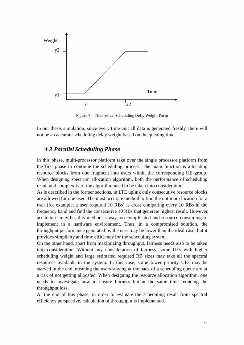
making process. Figure 7 shows the form of linear equation for theoretical

scheduling delay weight calculation.

25

Figure 7 Theoretical Scheduling Delay Weight Form

In our thesis simulation, since every time unit all data is generated freshly, there will

not be an accurate scheduling delay weight based on the queuing time.

4.3 Parallel Scheduling Phase

In this phase, multi-processor platform take over the single processor platform from

the first phase to continue the scheduling process. The main function is allocating

resource blocks from one fragment into users within the corresponding UE group.

When designing spectrum allocation algorithm, both the performance of scheduling

result and complexity of the algorithm need to be taken into consideration.

As is described in the former sections, in LTE uplink only consecutive resource blocks

are allowed for one user. The most accurate method to find the optimum location for a

user (for example, a user required 10 RBs) is cross comparing every 10 RBs in the

frequency band and find the consecutive 10 RBs that generate highest result. However,

accurate it may be, this method is way too complicated and resource consuming to

implement in a hardware environment. Thus, in a compromised solution, the

throughput performance generated by the user may be lower than the ideal case, but it

provides simplicity and time efficiency for the scheduling system.

On the other hand, apart from maximizing throughput, fairness needs also to be taken

into consideration. Without any consideration of fairness, some UEs with higher

scheduling weight and large estimated required RB sizes may take all the spectral

resources available in the system. In this case, some lower priority UEs may be

starved in the end, meaning the users staying at the back of a scheduling queue are at

a risk of not getting allocated. When designing the resource allocation algorithm, one

needs to investigate how to ensure fairness but at the same time reducing the

throughput loss.

At the end of this phase, in order to evaluate the scheduling result from spectral

efficiency perspective, calculation of throughput is implemented.

y2

y1

x1 x2

Weight

Time

26

4.3.1 Throughput Calculation

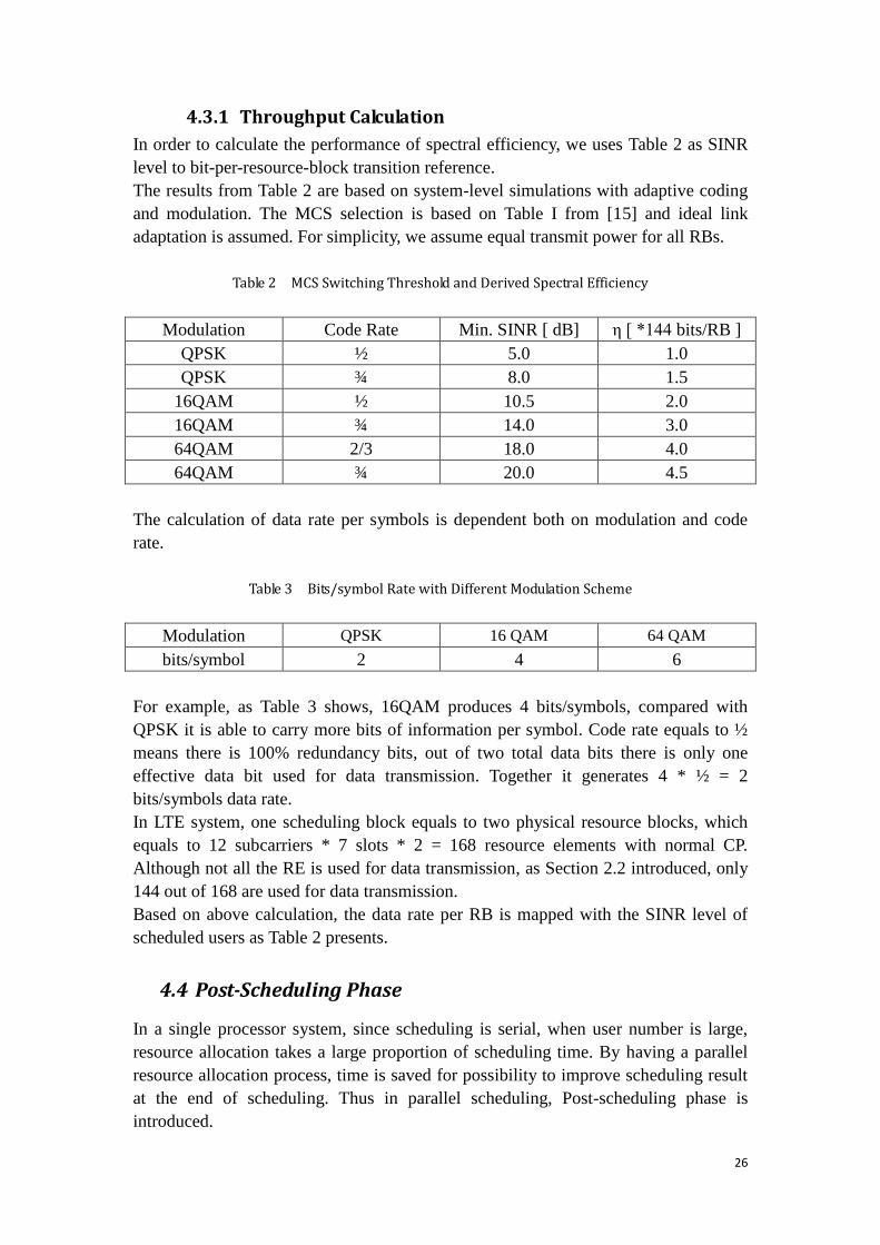
In order to calculate the performance of spectral efficiency, we uses Table 2 as SINR

level to bit-per-resource-block transition reference.

The results from Table 2 are based on system-level simulations with adaptive coding

and modulation. The MCS selection is based on Table I from [15] and ideal link

adaptation is assumed. For simplicity, we assume equal transmit power for all RBs.

Table 2 MCS Switching Threshold and Derived Spectral Efficiency

Modulation Code Rate Min. SINR [ dB] η [ *144 bits/RB ]

QPSK ½ 5.0 1.0

QPSK ¾ 8.0 1.5

16QAM ½ 10.5 2.0

16QAM ¾ 14.0 3.0

64QAM 2/3 18.0 4.0

64QAM ¾ 20.0 4.5

The calculation of data rate per symbols is dependent both on modulation and code

rate.

Table 3 Bits/symbol Rate with Different Modulation Scheme

Modulation QPSK 16 QAM 64 QAM

bits/symbol 2 4 6

For example, as Table 3 shows, 16QAM produces 4 bits/symbols, compared with

QPSK it is able to carry more bits of information per symbol. Code rate equals to ½

means there is 100% redundancy bits, out of two total data bits there is only one

effective data bit used for data transmission. Together it generates 4 * ½ = 2

bits/symbols data rate.

In LTE system, one scheduling block equals to two physical resource blocks, which

equals to 12 subcarriers * 7 slots * 2 = 168 resource elements with normal CP.

Although not all the RE is used for data transmission, as Section 2.2 introduced, only

144 out of 168 are used for data transmission.

Based on above calculation, the data rate per RB is mapped with the SINR level of

scheduled users as Table 2 presents.

4.4 Post-Scheduling Phase

In a single processor system, since scheduling is serial, when user number is large,

resource allocation takes a large proportion of scheduling time. By having a parallel

resource allocation process, time is saved for possibility to improve scheduling result

at the end of scheduling. Thus in parallel scheduling, Post-scheduling phase is

introduced.

27

In this phase, there is no UE Group or frequency fragment concept. The reason for

this is that users would have more freedom to extend their current resource allocation

or to be reallocated. However, due to this change, this phase may generate lower time

efficiency than Phase 2, users has to wait for previous users to be scheduled first.

Thus, the number of users needed to be reallocated or modified should not be too

large. Keeping the algorithm simple and efficient is important in phase 3, some

compromise between time saving and throughput improvement is needed.

28

5 Scheduling Algorithm

This chapter is designed to give a detailed description regarding all the considered

scheduling algorithms. In order to explain the differences between implemented

solutions, first 4 sections are given for explaining different solutions we used in each

scheduling phases. 5.1 is used for serial scheduling description, 5.2 is presenting the

different solutions used in pre-scheduling phase, followed by 5.3 and 5.4 that

represent the parallel scheduling and post-scheduling phase respectively.

5.1 Serial Scheduling

Since the parallel scheduling algorithm will be compared and evaluated with the serial

process on time consumption and throughput improvement, the first simulation will

run in serial scheduling algorithm.

The serial scheduling process contains only one phase, in order to facilitate the

evaluation of the scheduling performance later, the resource allocation method is set

to be the same in serial scheduling and paralleled scheduling. However, there is no

fragment and group concept in serial scheduling.

The focus of compression between serial and parallel scheduling will be put on time

and throughput tradeoff under the same simulation scenario and settings. The result of

the serial scheduling will be presented in the next chapter when analyzing the

performance of parallel scheduling.

5.2 Pre-Scheduling Phase

In parallel scheduling process, two methods will be presented for dividing both

Frequency Fragments and UE Groups. The two steps in Phase 1 will be labeled as

Phase 1-1 and Phase 1-2 respectively. Methods in each step are presented using the

name of „simple scheme‟ and „advanced scheme‟, a detailed explanation of how each

method works will follow below.

29

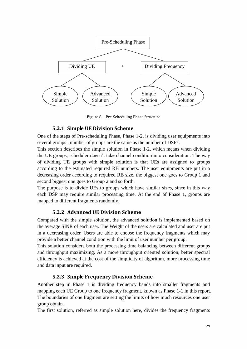
Figure 8 Pre-Scheduling Phase Structure

5.2.1 Simple UE Division Scheme

One of the steps of Pre-scheduling Phase, Phase 1-2, is dividing user equipments into

several groups , number of groups are the same as the number of DSPs.

This section describes the simple solution in Phase 1-2, which means when dividing

the UE groups, scheduler doesn‟t take channel condition into consideration. The way

of dividing UE groups with simple solution is that UEs are assigned to groups

according to the estimated required RB numbers. The user equipments are put in a

decreasing order according to required RB size, the biggest one goes to Group 1 and

second biggest one goes to Group 2 and so forth.

The purpose is to divide UEs to groups which have similar sizes, since in this way

each DSP may require similar processing time. At the end of Phase 1, groups are

mapped to different fragments randomly.

5.2.2 Advanced UE Division Scheme

Compared with the simple solution, the advanced solution is implemented based on

the average SINR of each user. The Weight of the users are calculated and user are put

in a decreasing order. Users are able to choose the frequency fragments which may

provide a better channel condition with the limit of user number per group.

This solution considers both the processing time balancing between different groups

and throughput maximizing. As a more throughput oriented solution, better spectral

efficiency is achieved at the cost of the simplicity of algorithm, more processing time

and data input are required.

5.2.3 Simple Frequency Division Scheme

Another step in Phase 1 is dividing frequency bands into smaller fragments and

mapping each UE Group to one frequency fragment, known as Phase 1-1 in this report.

The boundaries of one fragment are setting the limits of how much resources one user

group obtain.

The first solution, referred as simple solution here, divides the frequency fragments

Pre-Scheduling Phase

Dividing UE Dividing Frequency

Advanced

Solution

Advanced

Solution

Simple

Solution

Simple

Solution

+

30

regardless of UE Groups sizes. Frequency resources are divided evenly into fragments

according to the processor number.

5.2.4 Advanced Frequency Division Scheme

The advanced scheme for dividing frequency band is based on the assumption that if a

bigger group is assigned to a larger fragment it may make better use of the frequency

resources and fewer resources will be wasted. And in this way, the users in big groups

have more available frequency resource to choose from, which may improve spectral

efficiency as well. Thus, different from the simple solution, all fragments sizes are not

the same , i.e. they are adjusted according to the group sizes.

5.3 Parallel Scheduling Phase

In the second phase, in a multi-core environment, each processor obtains one UE list

and the corresponding fragment, allocating users into frequency fragment.

In this phase, two solutions are presented. One is designed from maximizing fairness

perspective and called fairness-oriented solution. Another one is from maximizing

throughput perspective and named as throughput-oriented solution.

The following sections will explain more in details about the tradeoff between these

two factors.

5.3.1 Maximum Throughput

From a maximizing throughput perspective, since the users with better channel

condition level may generate better spectral efficiency, such users are allowed to take

as many resources as they require. However, in this case, the inevitable flaw is the

unfairness. Some users within the same group as the greedy UEs may lose their

chance for frequency resources, thus „starved‟ in this scheduling time unit. But in this

throughput-oriented solution, fairness is not our main concern. If some users are

starved because the better performed users take all the resources, they will be

removed from list at the end of scheduling process.

5.3.2 Maximum Fairness

On the contrary of the above throughput-oriented solution, the second scheme is

named as „fairness-oriented solution‟, which is proposed from a fairness point of view.

During each simulation, the generated user equipments will be granted with at least

one resource block in the system. It means with „fairness-oriented solution‟ no user is

going to be starved. To ensure fairness among all the users, some “big” users need to

sacrifice some required RBs. The scheduler will only satisfy part of their requirements

when allocating resources.

5.4 Post-Scheduling Phase

As the last phase in the scheduling process, post-scheduling phase is the last chance to

improve scheduling performance. It is possible to improve the spectral efficiency by

31

extending the current resource allocation or by reallocating users in new locations.

However, as single processor platform it‟s important to keep the algorithm simple and

effective and also hold the number of rescheduled UEs as low as possible.

In the below sections, we present two alternative methods.

5.4.1 Simple Post-Scheduling Phase

The first solution, known as Phase 3-1, is aimed for higher throughput performance

based on a simple modification on assigned UEs. In order to minimize the complexity,

no reallocation is implemented but only extending the resource allocation for

scheduled users.

Extending current resource allocation means, due to different reasons a user may only

get part of their required RB, if there are available RBs adjacent to its current

allocation, it will make use of these resources after this step.

5.4.2 Advanced Post-Scheduling Phase

The advanced alternative for post-scheduling phase consists of two separated steps,

and both are with higher complexity than the simple solution. All the post-scheduling

steps are isolated from each other, and it is possible to implement independently. In

advanced solutions, it is possible to reallocate the users at new locations for higher

throughput.

The difference between two steps is that Phase 3-2 is reallocating user to a new

location that provides more available frequency resources, and Phase 3-3 moves a

user because the new location provides better channel conditions.

More frequency resources means, in the current location one user may get 10 RBs, but

in the new location it may get 15 RBs available

32

6 Performance Evaluation

6.1 Simulation Scenarios

In order to provide a better picture of performed simulations in this thesis and for the

facility of result and solution chapter, this section will be used to list different

performed simulation settings.

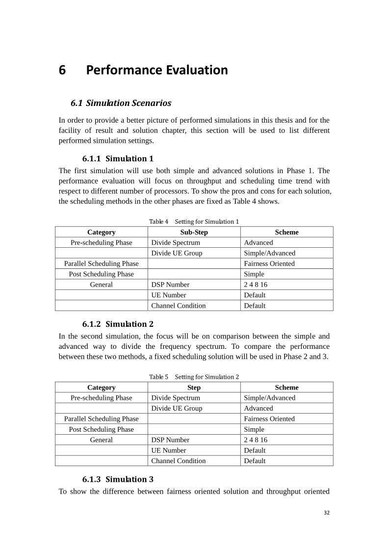
6.1.1 Simulation 1

The first simulation will use both simple and advanced solutions in Phase 1. The

performance evaluation will focus on throughput and scheduling time trend with

respect to different number of processors. To show the pros and cons for each solution,

the scheduling methods in the other phases are fixed as Table 4 shows.

Table 4 Setting for Simulation 1

Category Sub-Step Scheme

Pre-scheduling Phase Divide Spectrum Advanced

Divide UE Group Simple/Advanced

Parallel Scheduling Phase Fairness Oriented

Post Scheduling Phase Simple

General DSP Number 2 4 8 16

UE Number Default

Channel Condition Default

6.1.2 Simulation 2

In the second simulation, the focus will be on comparison between the simple and

advanced way to divide the frequency spectrum. To compare the performance

between these two methods, a fixed scheduling solution will be used in Phase 2 and 3.

Table 5 Setting for Simulation 2

Category Step Scheme

Pre-scheduling Phase Divide Spectrum Simple/Advanced

Divide UE Group Advanced

Parallel Scheduling Phase Fairness Oriented

Post Scheduling Phase Simple

General DSP Number 2 4 8 16

UE Number Default

Channel Condition Default

6.1.3 Simulation 3

To show the difference between fairness oriented solution and throughput oriented

33

solution for resource allocation, in simulation 3 we will focus on Phase 2. In Phase 1

and 3, the methods will be used as Table 6 shows. To give a more elaborate picture of

these two solutions, the result will be presented from different perspectives. The

setting for generated UE number is different from other performed simulation as well.

Table 6 Setting for Simulation 3

Category Step Scheme

Pre-scheduling Phase Divide Spectrum Advanced

Divide UE Group Advanced

Parallel Scheduling Phase Fairness/Throughput

Oriented

Post Scheduling Phase Simple

General DSP Number 2 4 8 16

UE Number Fixed number: 5 10 15 20

Channel Condition Default

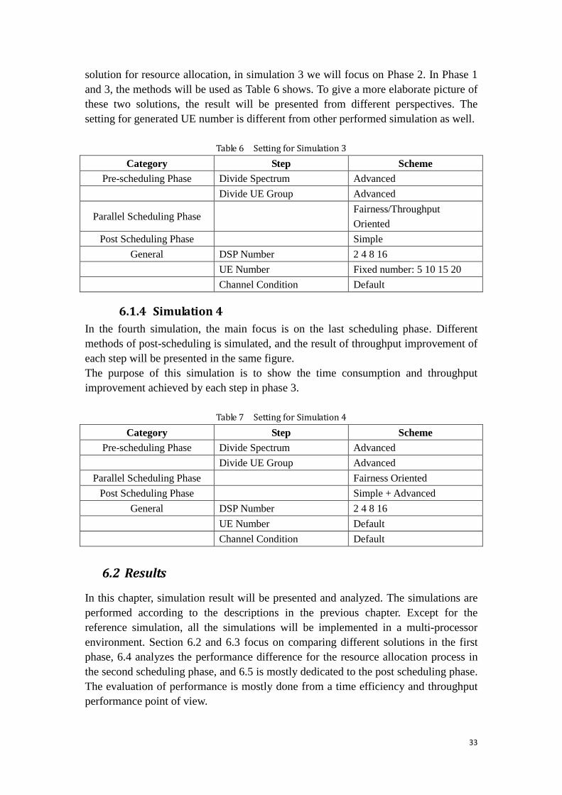
6.1.4 Simulation 4

In the fourth simulation, the main focus is on the last scheduling phase. Different

methods of post-scheduling is simulated, and the result of throughput improvement of

each step will be presented in the same figure.

The purpose of this simulation is to show the time consumption and throughput

improvement achieved by each step in phase 3.

Table 7 Setting for Simulation 4

Category Step Scheme

Pre-scheduling Phase Divide Spectrum Advanced

Divide UE Group Advanced

Parallel Scheduling Phase Fairness Oriented

Post Scheduling Phase Simple + Advanced

General DSP Number 2 4 8 16

UE Number Default

Channel Condition Default

6.2 Results

In this chapter, simulation result will be presented and analyzed. The simulations are

performed according to the descriptions in the previous chapter. Except for the

reference simulation, all the simulations will be implemented in a multi-processor

environment. Section 6.2 and 6.3 focus on comparing different solutions in the first

phase, 6.4 analyzes the performance difference for the resource allocation process in

the second scheduling phase, and 6.5 is mostly dedicated to the post scheduling phase.

The evaluation of performance is mostly done from a time efficiency and throughput

performance point of view.

34

6.2.1 Reference Simulation

First, we present the result generated with the Serial Scheduling algorithm with both

throughput maximizing and fairness maximizing resource allocation schemes.

Table 8 shows the results from three perspectives for each simulation. By introducing

the definition and meaning of each item, we give a general overview of how the

performance is evaluated and analyzed for all the performed simulations.

„Spectral Efficiency‟ tables show the throughput performances from each scheme, the

values are affected by two factors. First one is the number of resource blocks assigned

during each TTI, and the second one is channel condition of the assigned resource

blocks.

Based on the mapping from SINR value to data rate introduced in Table 2, the

throughput of a certain user can be calculated.

First, the average SINR of the user is calculated base on the resource blocks

he gets.

Table 2 provides the mapping from SINR value to the estimated data rate per

RB generated from ideal link adaptation. Using the average SINR value of one

user to find the corresponding data rate per RB, multiply with the number of

RBs each user gets, the total throughput of this user can be obtained.

The throughput presents the amount of data each user can send during one TTI. The

unit for throughput is (*144 bits/ms) in all the performed simulation.

For the „ Resource Assignment Efficiency‟ in Table 8, „NrOfUnassignedUE‟ is an

indicator of the number of starved UE during each TTI. Every TTI the user number is

generated randomly from 4-16, and in this example on average 0.866 user doesn‟t get

any frequency resource. „NrOfUnassignedRequiredRBs‟ stands for the sum of RBs

resources which are not assigned during one TTI. It means among the total 100 RBs

in this simulation environment, 28.5 are left unused on average.

The „Time Efficiency‟ in Table 8 represents the amount of time consumed to finish

each scheduling process. As we explained before, in the simulation environment time

is based on Matlab simulation, which shows the differences of complexity when

running different simulation cases. For this reason, the unit of time in this report will

not be presented, since as long as it is able to present the comparison of time

improvement, the absolute value of time in this report is not of concern.

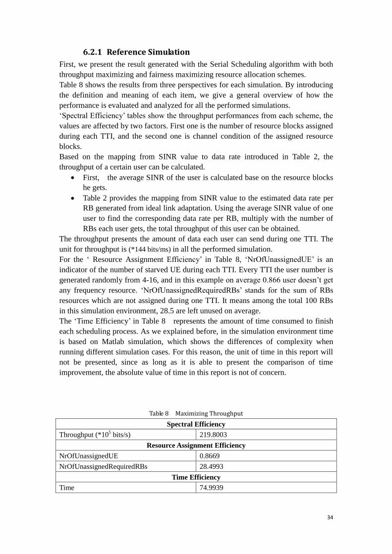
Table 8 Maximizing Throughput

Spectral Efficiency

Throughput (*105 bits/s) 219.8003

Resource Assignment Efficiency

NrOfUnassignedUE 0.8669

NrOfUnassignedRequiredRBs 28.4993

Time Efficiency

Time 74.9939

35

Table 9 Maximizing Fairness

Spectral Efficiency

Throughput (*105 bits/s) 186.4233

Transmission Efficiency

NrOfUnassignedUE 0

NrOfUnassignedRequiredRBs 35.0402

Time Efficiency

Time 91.5848

In these two cases, we can observe that the throughput-oriented solution generates

much higher user data rate than the fairness-oriented solution. This result confirms our

earlier analysis, that in order to keep fairness between different users, throughput

performance will be decreased. From „NrOfUnassignedUE‟ figure we can see 0

instead of 0.8669 users are starved during each TTI, the fairness performance is

improved by implementing fairness-oriented solution. The increase

„NrOfUnassignedRequiredRBs‟ may be due to the reason that UEs are restricted to

transmit only part of their requirements for the purpose of saving more frequency

resource for low priority users. From this result we can see the fairness-oriented

solution increases fairness among different users, however, it may also result in

reducing the total utilization of frequency resource. Regarding the time consumption

between these two cases, fairness-oriented solution brings more complexity and

consumes more time than throughput-oriented solution.

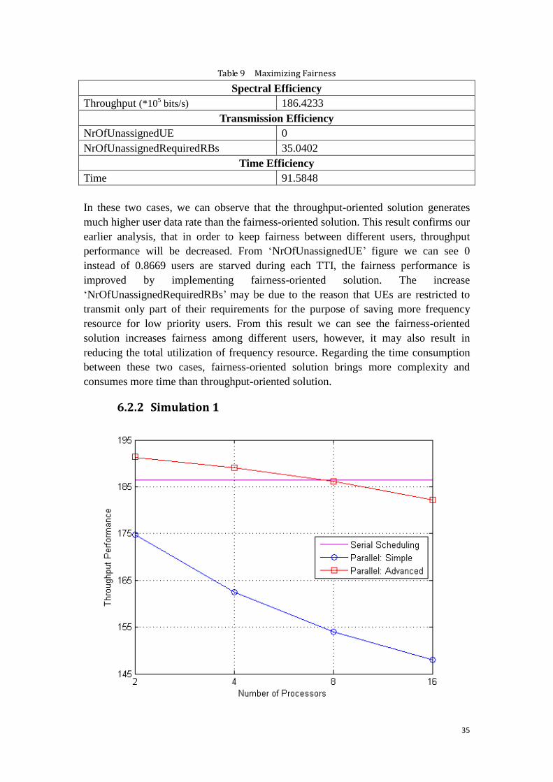
6.2.2 Simulation 1

36

Figure 9 Throughput trend with different NrOfDSPs

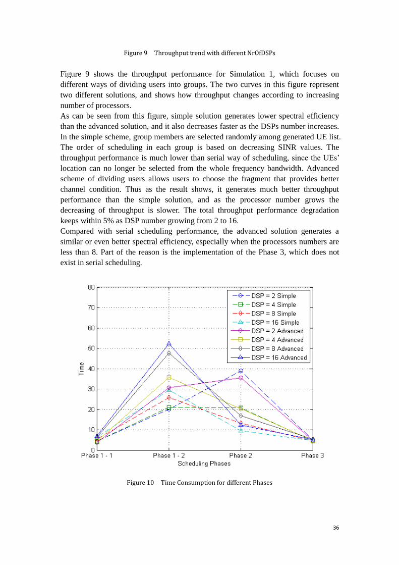
Figure 9 shows the throughput performance for Simulation 1, which focuses on

different ways of dividing users into groups. The two curves in this figure represent

two different solutions, and shows how throughput changes according to increasing

number of processors.

As can be seen from this figure, simple solution generates lower spectral efficiency

than the advanced solution, and it also decreases faster as the DSPs number increases.

In the simple scheme, group members are selected randomly among generated UE list.

The order of scheduling in each group is based on decreasing SINR values. The

throughput performance is much lower than serial way of scheduling, since the UEs‟

location can no longer be selected from the whole frequency bandwidth. Advanced

scheme of dividing users allows users to choose the fragment that provides better

channel condition. Thus as the result shows, it generates much better throughput

performance than the simple solution, and as the processor number grows the

decreasing of throughput is slower. The total throughput performance degradation

keeps within 5% as DSP number growing from 2 to 16.

Compared with serial scheduling performance, the advanced solution generates a

similar or even better spectral efficiency, especially when the processors numbers are

less than 8. Part of the reason is the implementation of the Phase 3, which does not

exist in serial scheduling.

Figure 10 Time Consumption for different Phases

37

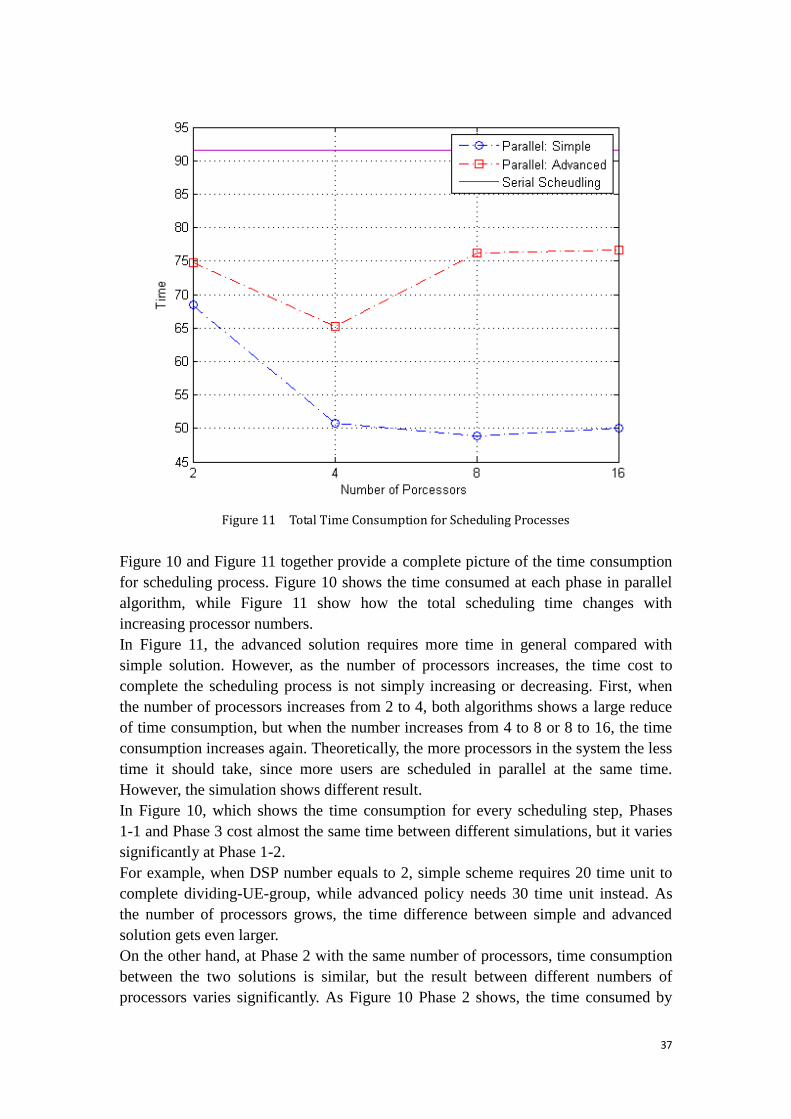
Figure 11 Total Time Consumption for Scheduling Processes

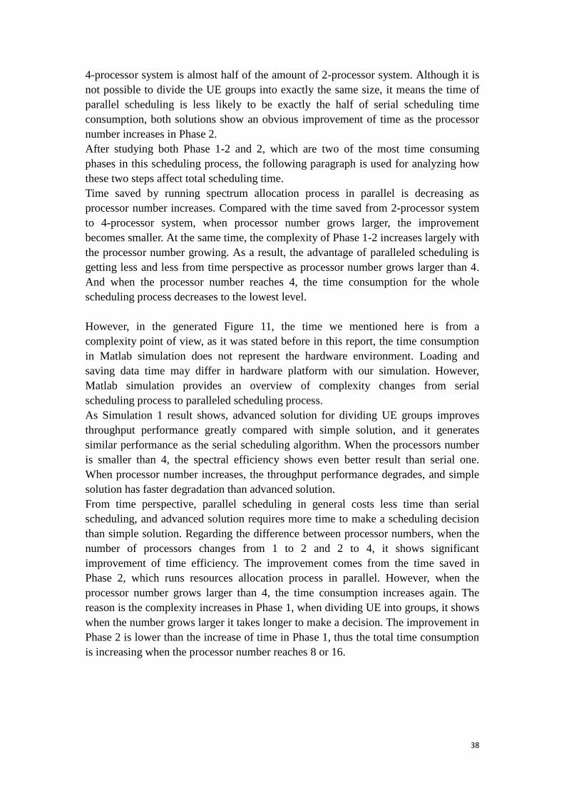
Figure 10 and Figure 11 together provide a complete picture of the time consumption

for scheduling process. Figure 10 shows the time consumed at each phase in parallel

algorithm, while Figure 11 show how the total scheduling time changes with

increasing processor numbers.

In Figure 11, the advanced solution requires more time in general compared with

simple solution. However, as the number of processors increases, the time cost to

complete the scheduling process is not simply increasing or decreasing. First, when

the number of processors increases from 2 to 4, both algorithms shows a large reduce

of time consumption, but when the number increases from 4 to 8 or 8 to 16, the time

consumption increases again. Theoretically, the more processors in the system the less

time it should take, since more users are scheduled in parallel at the same time.

However, the simulation shows different result.

In Figure 10, which shows the time consumption for every scheduling step, Phases

1-1 and Phase 3 cost almost the same time between different simulations, but it varies

significantly at Phase 1-2.

For example, when DSP number equals to 2, simple scheme requires 20 time unit to

complete dividing-UE-group, while advanced policy needs 30 time unit instead. As

the number of processors grows, the time difference between simple and advanced

solution gets even larger.

On the other hand, at Phase 2 with the same number of processors, time consumption

between the two solutions is similar, but the result between different numbers of

processors varies significantly. As Figure 10 Phase 2 shows, the time consumed by

38

4-processor system is almost half of the amount of 2-processor system. Although it is

not possible to divide the UE groups into exactly the same size, it means the time of

parallel scheduling is less likely to be exactly the half of serial scheduling time

consumption, both solutions show an obvious improvement of time as the processor

number increases in Phase 2.

After studying both Phase 1-2 and 2, which are two of the most time consuming

phases in this scheduling process, the following paragraph is used for analyzing how

these two steps affect total scheduling time.

Time saved by running spectrum allocation process in parallel is decreasing as

processor number increases. Compared with the time saved from 2-processor system

to 4-processor system, when processor number grows larger, the improvement

becomes smaller. At the same time, the complexity of Phase 1-2 increases largely with

the processor number growing. As a result, the advantage of paralleled scheduling is

getting less and less from time perspective as processor number grows larger than 4.

And when the processor number reaches 4, the time consumption for the whole

scheduling process decreases to the lowest level.

However, in the generated Figure 11, the time we mentioned here is from a

complexity point of view, as it was stated before in this report, the time consumption

in Matlab simulation does not represent the hardware environment. Loading and

saving data time may differ in hardware platform with our simulation. However,

Matlab simulation provides an overview of complexity changes from serial

scheduling process to paralleled scheduling process.

As Simulation 1 result shows, advanced solution for dividing UE groups improves

throughput performance greatly compared with simple solution, and it generates

similar performance as the serial scheduling algorithm. When the processors number

is smaller than 4, the spectral efficiency shows even better result than serial one.

When processor number increases, the throughput performance degrades, and simple

solution has faster degradation than advanced solution.

From time perspective, parallel scheduling in general costs less time than serial

scheduling, and advanced solution requires more time to make a scheduling decision

than simple solution. Regarding the difference between processor numbers, when the

number of processors changes from 1 to 2 and 2 to 4, it shows significant

improvement of time efficiency. The improvement comes from the time saved in

Phase 2, which runs resources allocation process in parallel. However, when the

processor number grows larger than 4, the time consumption increases again. The

reason is the complexity increases in Phase 1, when dividing UE into groups, it shows

when the number grows larger it takes longer to make a decision. The improvement in

Phase 2 is lower than the increase of time in Phase 1, thus the total time consumption

is increasing when the processor number reaches 8 or 16.

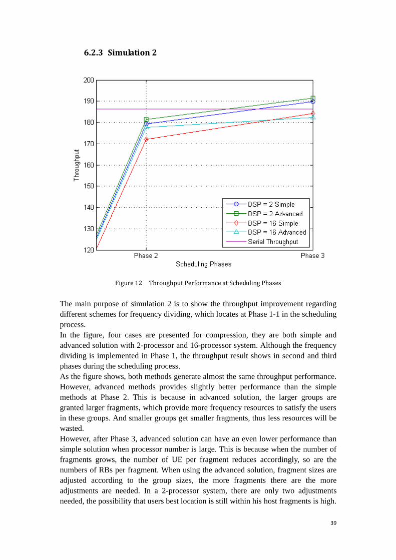
39

6.2.3 Simulation 2

Figure 12 Throughput Performance at Scheduling Phases

The main purpose of simulation 2 is to show the throughput improvement regarding

different schemes for frequency dividing, which locates at Phase 1-1 in the scheduling

process.

In the figure, four cases are presented for compression, they are both simple and

advanced solution with 2-processor and 16-processor system. Although the frequency

dividing is implemented in Phase 1, the throughput result shows in second and third

phases during the scheduling process.

As the figure shows, both methods generate almost the same throughput performance.

However, advanced methods provides slightly better performance than the simple

methods at Phase 2. This is because in advanced solution, the larger groups are

granted larger fragments, which provide more frequency resources to satisfy the users

in these groups. And smaller groups get smaller fragments, thus less resources will be

wasted.

However, after Phase 3, advanced solution can have an even lower performance than

simple solution when processor number is large. This is because when the number of

fragments grows, the number of UE per fragment reduces accordingly, so are the

numbers of RBs per fragment. When using the advanced solution, fragment sizes are

adjusted according to the group sizes, the more fragments there are the more

adjustments are needed. In a 2-processor system, there are only two adjustments

needed, the possibility that users best location is still within his host fragments is high.

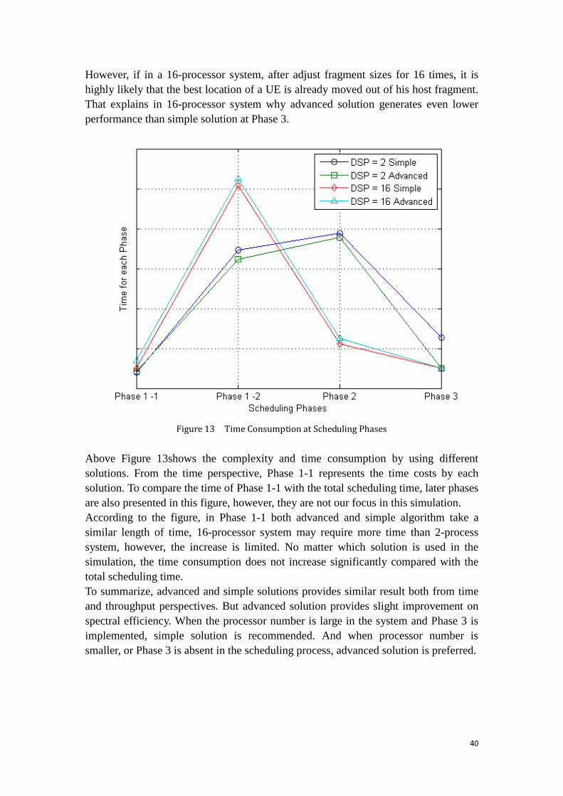
40

However, if in a 16-processor system, after adjust fragment sizes for 16 times, it is

highly likely that the best location of a UE is already moved out of his host fragment.

That explains in 16-processor system why advanced solution generates even lower

performance than simple solution at Phase 3.

Figure 13 Time Consumption at Scheduling Phases

Above Figure 13shows the complexity and time consumption by using different

solutions. From the time perspective, Phase 1-1 represents the time costs by each

solution. To compare the time of Phase 1-1 with the total scheduling time, later phases

are also presented in this figure, however, they are not our focus in this simulation.

According to the figure, in Phase 1-1 both advanced and simple algorithm take a

similar length of time, 16-processor system may require more time than 2-process

system, however, the increase is limited. No matter which solution is used in the

simulation, the time consumption does not increase significantly compared with the

total scheduling time.

To summarize, advanced and simple solutions provides similar result both from time

and throughput perspectives. But advanced solution provides slight improvement on

spectral efficiency. When the processor number is large in the system and Phase 3 is

implemented, simple solution is recommended. And when processor number is

smaller, or Phase 3 is absent in the scheduling process, advanced solution is preferred.

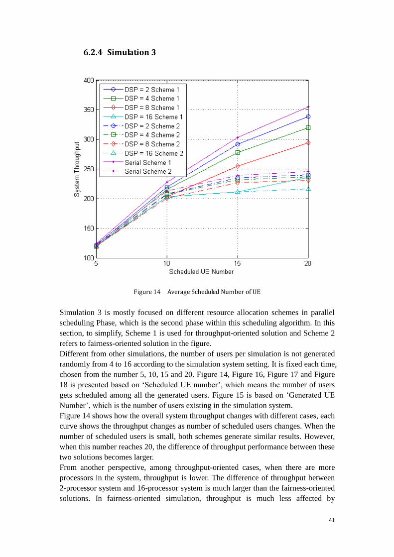
41

6.2.4 Simulation 3

Figure 14 Average Scheduled Number of UE

Simulation 3 is mostly focused on different resource allocation schemes in parallel

scheduling Phase, which is the second phase within this scheduling algorithm. In this

section, to simplify, Scheme 1 is used for throughput-oriented solution and Scheme 2

refers to fairness-oriented solution in the figure.

Different from other simulations, the number of users per simulation is not generated

randomly from 4 to 16 according to the simulation system setting. It is fixed each time,

chosen from the number 5, 10, 15 and 20. Figure 14, Figure 16, Figure 17 and Figure

18 is presented based on „Scheduled UE number‟, which means the number of users

gets scheduled among all the generated users. Figure 15 is based on „Generated UE

Number‟, which is the number of users existing in the simulation system.

Figure 14 shows how the overall system throughput changes with different cases, each

curve shows the throughput changes as number of scheduled users changes. When the

number of scheduled users is small, both schemes generate similar results. However,

when this number reaches 20, the difference of throughput performance between these

two solutions becomes larger.

From another perspective, among throughput-oriented cases, when there are more

processors in the system, throughput is lower. The difference of throughput between

2-processor system and 16-processor system is much larger than the fairness-oriented

solutions. In fairness-oriented simulation, throughput is much less affected by

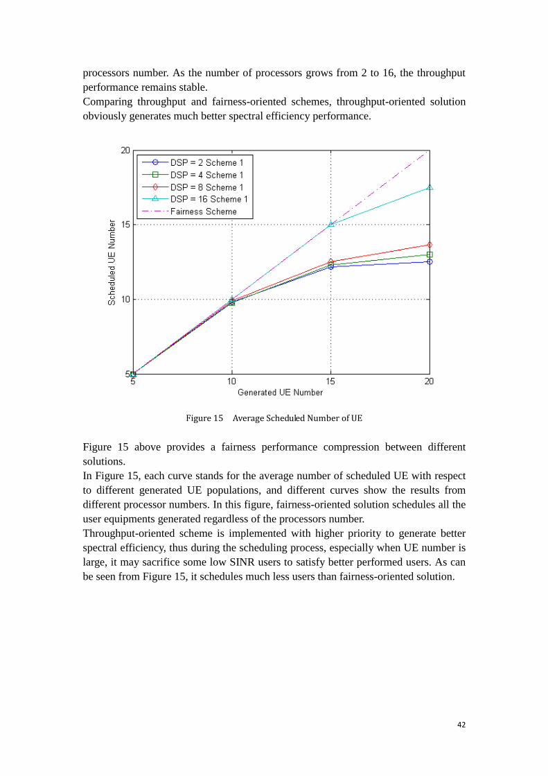
42

processors number. As the number of processors grows from 2 to 16, the throughput

performance remains stable.

Comparing throughput and fairness-oriented schemes, throughput-oriented solution

obviously generates much better spectral efficiency performance.

Figure 15 Average Scheduled Number of UE

Figure 15 above provides a fairness performance compression between different

solutions.

In Figure 15, each curve stands for the average number of scheduled UE with respect

to different generated UE populations, and different curves show the results from

different processor numbers. In this figure, fairness-oriented solution schedules all the

user equipments generated regardless of the processors number.

Throughput-oriented scheme is implemented with higher priority to generate better

spectral efficiency, thus during the scheduling process, especially when UE number is

large, it may sacrifice some low SINR users to satisfy better performed users. As can

be seen from Figure 15, it schedules much less users than fairness-oriented solution.

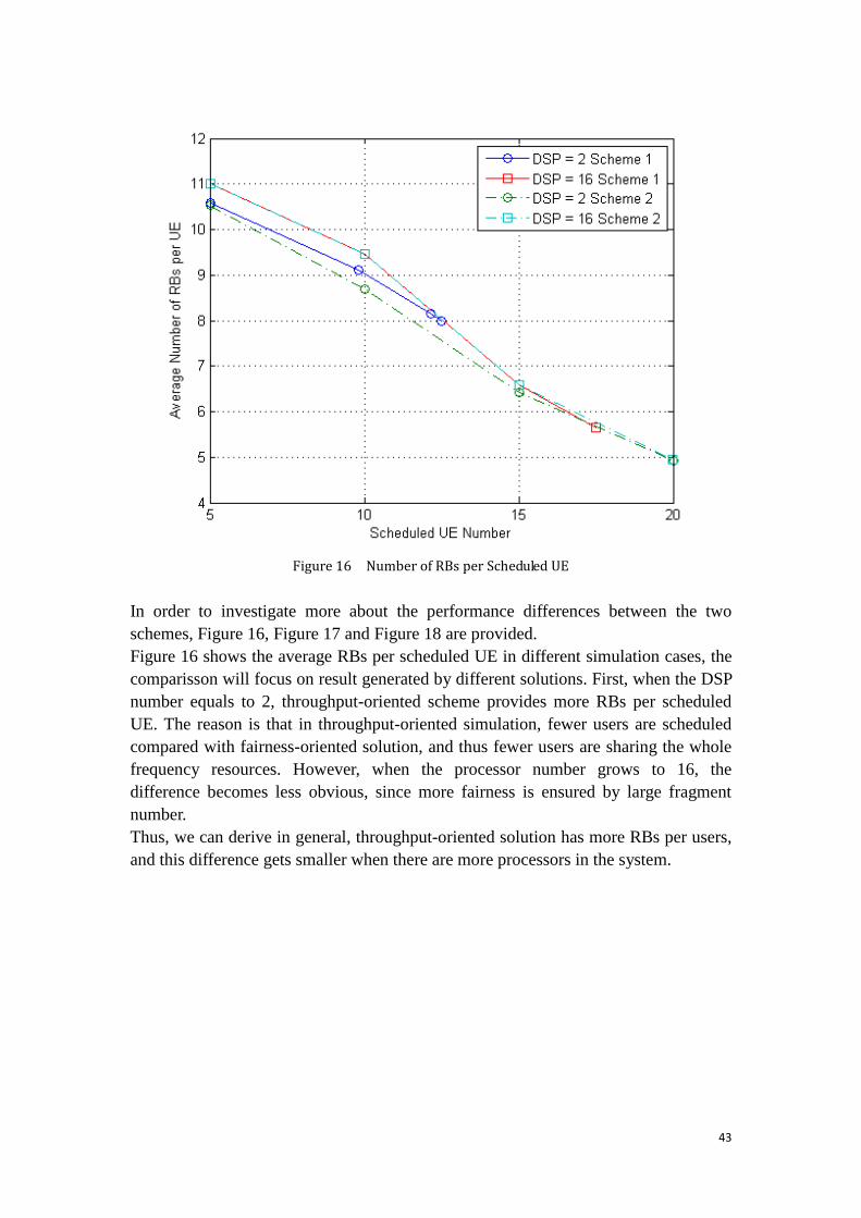
43

Figure 16 Number of RBs per Scheduled UE

In order to investigate more about the performance differences between the two

schemes, Figure 16, Figure 17 and Figure 18 are provided.

Figure 16 shows the average RBs per scheduled UE in different simulation cases, the

comparisson will focus on result generated by different solutions. First, when the DSP

number equals to 2, throughput-oriented scheme provides more RBs per scheduled

UE. The reason is that in throughput-oriented simulation, fewer users are scheduled

compared with fairness-oriented solution, and thus fewer users are sharing the whole

frequency resources. However, when the processor number grows to 16, the

difference becomes less obvious, since more fairness is ensured by large fragment

number.

Thus, we can derive in general, throughput-oriented solution has more RBs per users,

and this difference gets smaller when there are more processors in the system.

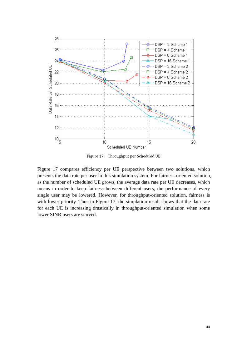
44

Figure 17 Throughput per Scheduled UE

Figure 17 compares efficiency per UE perspective between two solutions, which

presents the data rate per user in this simulation system. For fairness-oriented solution,

as the number of scheduled UE grows, the average data rate per UE decreases, which

means in order to keep fairness between different users, the performance of every

single user may be lowered. However, for throughput-oriented solution, fairness is

with lower priority. Thus in Figure 17, the simulation result shows that the data rate

for each UE is increasing drastically in throughput-oriented simulation when some

lower SINR users are starved.

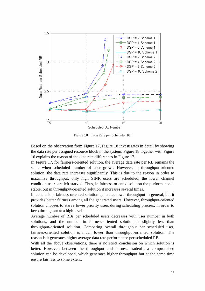
45

Figure 18 Data Rate per Scheduled RB

Based on the observation from Figure 17, Figure 18 investigates in detail by showing

the data rate per assigned resource block in the system. Figure 18 together with Figure

16 explains the reason of the data rate differences in Figure 17.

In Figure 17, for fairness-oriented solution, the average data rate per RB remains the

same when scheduled number of user grows. However, in throughput-oriented

solution, the data rate increases significantly. This is due to the reason in order to

maximize throughput, only high SINR users are scheduled, the lower channel

condition users are left starved. Thus, in fairness-oriented solution the performance is

stable, but in throughput-oriented solution it increases several times.

In conclusion, fairness-oriented solution generates lower throughput in general, but it

provides better fairness among all the generated users. However, throughput-oriented

solution chooses to starve lower priority users during scheduling process, in order to

keep throughput at a high level.

Average number of RBs per scheduled users decreases with user number in both

solutions, and the number in fairness-oriented solution is slightly less than

throughput-oriented solution. Comparing overall throughput per scheduled user,

fairness-oriented solution is much lower than throughput-oriented solution. The

reason is it generates higher average data rate performance per scheduled RB.

With all the above observations, there is no strict conclusion on which solution is

better. However, between the throughput and fairness tradeoff, a compromised

solution can be developed, which generates higher throughput but at the same time

ensure fairness to some extent.

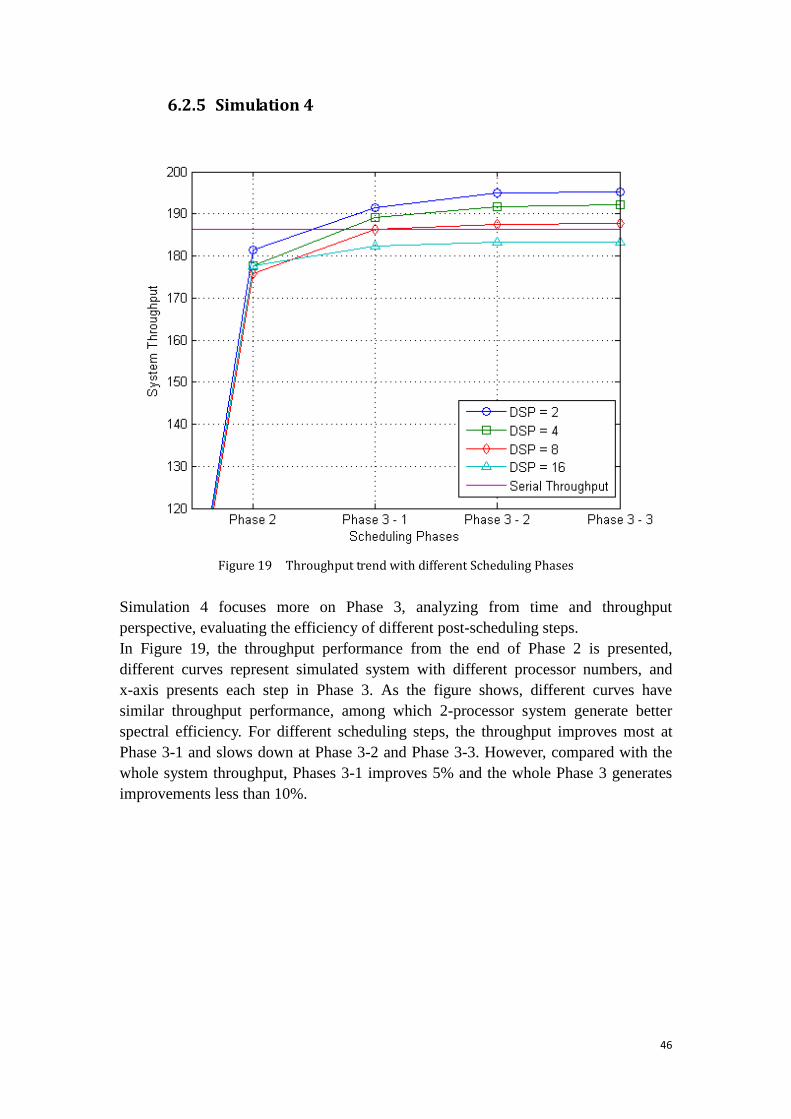
46

6.2.5 Simulation 4

Figure 19 Throughput trend with different Scheduling Phases

Simulation 4 focuses more on Phase 3, analyzing from time and throughput

perspective, evaluating the efficiency of different post-scheduling steps.

In Figure 19, the throughput performance from the end of Phase 2 is presented,

different curves represent simulated system with different processor numbers, and

x-axis presents each step in Phase 3. As the figure shows, different curves have

similar throughput performance, among which 2-processor system generate better

spectral efficiency. For different scheduling steps, the throughput improves most at

Phase 3-1 and slows down at Phase 3-2 and Phase 3-3. However, compared with the

whole system throughput, Phases 3-1 improves 5% and the whole Phase 3 generates

improvements less than 10%.

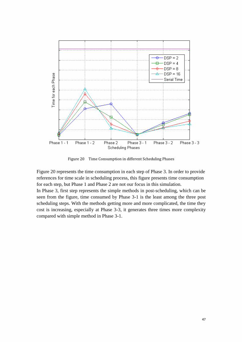
47

Figure 20 Time Consumption in different Scheduling Phases

Figure 20 represents the time consumption in each step of Phase 3. In order to provide

references for time scale in scheduling process, this figure presents time consumption

for each step, but Phase 1 and Phase 2 are not our focus in this simulation.

In Phase 3, first step represents the simple methods in post-scheduling, which can be

seen from the figure, time consumed by Phase 3-1 is the least among the three post

scheduling steps. With the methods getting more and more complicated, the time they

cost is increasing, especially at Phase 3-3, it generates three times more complexity

compared with simple method in Phase 3-1.

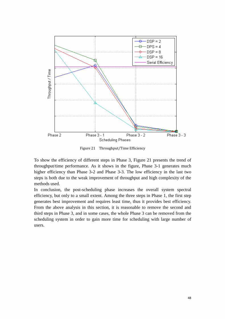
48

Figure 21 Throughput/Time Efficiency

To show the efficiency of different steps in Phase 3, Figure 21 presents the trend of

throughput/time performance. As it shows in the figure, Phase 3-1 generates much

higher efficiency than Phase 3-2 and Phase 3-3. The low efficiency in the last two

steps is both due to the weak improvement of throughput and high complexity of the

methods used.

In conclusion, the post-scheduling phase increases the overall system spectral

efficiency, but only to a small extent. Among the three steps in Phase 1, the first step

generates best improvement and requires least time, thus it provides best efficiency.

From the above analysis in this section, it is reasonable to remove the second and

third steps in Phase 3, and in some cases, the whole Phase 3 can be removed from the

scheduling system in order to gain more time for scheduling with large number of

users.

49

7 Discussions

7.1 Conclusion

Based on the simulation result and analysis presented in the last chapter, in this

section, pros and cons of different solutions in each phase will be discussed in pairs,

and conclusions will be drawn.

In Phase 1-1, dividing frequency band into fragments, both solutions provide similar

results both in throughput and time perspective. However, advanced solution is able to

provide slight improvement on spectral efficiency. When the processor number is

large (8 or 16) in the simulation system and Phase 3 is implemented, simple solution

is recommended. And when processor number is smaller (2 or 4) or Phase 3 is absent

in the scheduling process, advanced solution is preferred.

In Phase 1-2, dividing UE groups, simple solution saves more time but generate lower

spectral efficiency, to be more specific, the throughput performance is 20% lower than

serial scheduling result. The advanced solution consumes more time but keeps a

similar throughput performance as serial scheduling. Both solutions are processing

faster than serial scheduling algorithm and when processor number is no bigger than 4

it generates better throughput and time performance than the cases when processor

number is larger. Thus, in the cases when time is more critical than throughput, simple

solution is recommended, but if throughput is the main concern, advance solution

provides better result. In both solutions, number of processor is recommended to be

no more than a certain number, this number depends on the simulation environment of

the system, however, in this thesis environment, it equals to 4.

In Phase 2, which is the resource allocation phase, fairness-oriented solution

schedules every generated user, thus it has higher fairness compared with

throughput-oriented solution, while the throughput-oriented solution provides better

spectral efficiency performance in general. Based on the throughput and fairness

tradeoff, there is no strict definition on which is the better solution. However, a

compromised solution can be developed, which may generate a throughput

performance between the results of two tested solutions and ensures fairness to some

extent.

In the last phase, among all the three steps tested, first step is able to improve

throughput by 10% and it shows a higher efficiency compared with following two

steps. It is reasonable to suggest removing the second and third steps in Phase 3 due to

their low efficiency. And in some time critical cases, the whole Phase 3 can be

removed from the scheduling system in order to gain more processing time for

scheduling with large number of users.

To summarize the conclusion, based on our simulation result, the current 3 Phases

structure of parallel scheduling algorithm is able to provide better throughput and time

efficiency compared with the serial scheduling algorithm. The details about

improvements brought by parallelism are not only dependent on the number of

50

processor in use, the number of generated users in system but also on throughput

fairness performance tradeoff. When the number of generated users in the system is

larger, the improvement of parallel scheduling algorithm is more obvious. Based on

the simulation settings in this thesis, the parallel scheduling algorithm with

4-processor platform is able to generate the same throughput performance with the

serial algorithm, and the time consumption is reduced by 30% in Matlab simulation.

However, the time consumption in this thesis simulation does not reflect the hardware

environment. Thus, it can not be used as a reference to describe the real time

improvement, the recommended number of processors in real system needs more

investigation built on hardware environment.

Above all, based on the simulation, the recommended solution in each phase is listed

as below.

In time critical cases, simple solution for dividing the UE groups and frequency

fragments are preferred, at the same time Phase 3 can be removed from the scheduling

system, or only step one in Phase 3 is recommended. In order to ensure a higher level

of fairness in the system, in Phase 2, fairness-oriented solution is a favorable choice.

If the system throughput is the main concern when choosing scheduling solutions,

advanced solutions are recommended in Phase 1, throughput-oriented scheme in

Phase 2 and first step in Phase 3.

7.2 Future Work

In this thesis scope, the most focus has been put on variation of scheduling methods in

different phases and the pros and cons of each combination. As a result, a simplified

simulation environment has been used with respect to traffic load and simulation

settings.

Time Domain Memory

This thesis is focusing on studying simulation performance from a frequency

domain point of view. During each scheduling time unit, this simulation

environment would generate required data all over again. However, it would

be an interesting path of investigation if the scheduling process simulation has

a UE memory in the time domain. The information of unsatisfied data can be

save for the next time unit, and the scheduling delay weight is increased due to

this prolonged scheduling time, which will grant this user higher priority to be

scheduled in the following TTI. The simulation will present a picture of how

this algorithm performed in the time domain.

Traffic Load

Some spectral efficiency performance improvement is not obvious after

post-scheduling process or difference is not fully shown between different

scheduling solutions, one of the reasons can be the traffic load used. There is

only one traffic load model in the simulation environment with one setting of

required RBs and generated user number. More obvious improvement will be

51

generated if a lager user number is used, and larger processor number is

implemented. And different required RBs setting would also generate a

different simulation performance.

Time Evaluation

The current time consumption is based on the simulation in Matlab. In general

it is an ideal and simplified simulation model. In a time perspective, the time

for loading and saving data in DSP is not taken into account, neither is some

setting up time needed in a hardware environment, thus is not 100 percent

accurate in time estimation and evaluation between serial and parallel

algorithm. The efficiency of post-scheduling phase can be reevaluated, so is

the time improvement brought by parallel scheduling. With a simulator that

has the exact same performance as current hardware implementation, the time

evaluation would be more accurate.

Above all, the result of parallel algorithm would be further verified by implementing

above suggested simulations.

52

8 References

[1] LTE eNodeB MAC Scheduler Introduction; Technical report, Ericsson, 2009.

[2] US Patent Application 20100284314 - Compressed Buffer Status Reports in LTE

[4] 3GPP TS 36.101; User Equipment (UE) radio transmission and reception (Release

8)

[5] 3GPP TS 36.211; Physical Channels and Modulation (Release 8)

[6] Lee S B, Choudhury S, Khoshnevis A, et al; Downlink MIMO with Frequency

Domain Packet Scheduling for 3GPP LTE; Proceedings of IEEE INFOCOM , 2009.

[7] Zyren J.; Overview of the 3GPP Long Term Evolution Physical Layer; Technical

report, Freescale Semiconductor, 2007.

[8] LTE - an introduction; Technical report, Ericsson, 2009.

[9] H. G. Myung, et al; Peak-to-average Power Ratio of Single Carrier FDMA Signals

with Pulse Shaping; Accepted to IEEE PIMRC‟06

[10] UMTS Long Term Evolution (LTE) Technology Introduction; Application Note,

Rohde & Schwarz

[11] Erik Dahlman, Stefan Parkvall, Johan skold, Per Beming; 3G Evolution, HSPA

and LTE for Mobile Broadband; Academic Press, Oxford, UK, second edition, 2008.

[12] Erik Dahlman, Stefan Parkvall, Johan skold; 4G LTE/LTE-Advanced for Mobile

Broadband; Academic Press, first Edition, 2011.[13] Mohammed Al-Rawi, Riku Jantti,

Johan Torsner, Mats Sagfors; On the Performance of Heuristic Opportunistic Scheduling

in the Uplink of 3G LTE Networks; Personal, Indoor and Mobile Radio

Communications, 2008.

[14] Maxime Pelcat, Jean-Francois Nezan, Slaheddine Aridhi; Adaptive Multicore

Scheduling for the LTE Uplink; Adaptive Hardware and Systems (AHS), 2010

NASA/ESA Conference

[15] IEEE DRAFT standard for local and metropolitan area networks part 16: Air

interface for fixed broadband wireless access systems; P802.16Rev2/D8, Dec. 2008.

[16] Hongkun Yang, Fengyuan Ren, Chuang Lin, Jiao Zhang; Frequency-Domain Packet

Scheduling for 3GPP LTE Uplink; INFOCOM, 2010 Proceedings IEEE

[17] Junsung Lim, Hyung G. Myung, Kyungjin Oh, David J. Goodman; Channel-Dependent

Scheduling of Uplink Single Carrier FDMA Systems; Vehicular Technology Conference,

2006. 2006 IEEE 64th

[18] Erik Dahlman, Anders Furuskär, Ylva Jading, Magnus Lindström and Stefan Parkvall;

Key features of the LTE radio interface; Technical report, Ericsson, 2008.

[19] Long Term Evolution Protocol Overview; White Paper; Freescale Semiconductor

[20] Hongwei Wang; CSI Measurement Offset Compensation Algorithms for Link and Rank

Adaptation in LTE; Master Thesis Report, Ericsson, 2010.

[21] R. Agrawal and V. Subramanian ”Optimality of Certain Channel Aware

Scheduling Policies,” Proc. of 2002 Allerton Conference on Communication, Control

and Computing, Oct. 2002.