Embed Size (px)
Citation preview

A Radio Resource Management Framework for the
3GPP LTE Uplink
By
Amira Mohamed Yehia Abdulhadi Afifi
B.Sc. in Electronics and Communications Engineering – Cairo University
A Thesis Submitted to the
Faculty of Engineering at Cairo University
in Partial Fulfillment of the
Requirements for the Degree of
Master of Science
in
Electronics and Electrical Communications Engineering
Faculty of Engineering, Cairo University
Giza, Egypt
2011

A Radio Resource Management Framework for the
3GPP LTE Uplink
By
Amira Mohamed Yehia Abdulhadi Afifi
B.Sc. in Electronics and Communications Engineering – Cairo University
A Thesis Submitted to the
Faculty of Engineering at Cairo University
in Partial Fulfillment of the
Requirements for the Degree of
Master of Science
in
Electronics and Electrical Communications Engineering
Supervised by
Prof. Dr. Khaled Mohamed Fouad Elsayed
Faculty of Engineering, Cairo University
Faculty of Engineering, Cairo University
Giza, Egypt
2011
A Radio Resource Management Framework for the
3GPP LTE Uplink
By
Amira Mohamed Yehia Abdulhadi Afifi
B.Sc. in Electronics and Communications Engineering – Cairo University
A Thesis Submitted to the
Faculty of Engineering at Cairo University
in Partial Fulfillment of the
Requirements for the Degree of
Master of Science
in
Electronics and Electrical Communications Engineering
Approved by the Examining Committee:
Prof. Dr. Salwa Hussain Elramly Member (Ain Shams University)
Prof. Dr. Mohamed Hazem Mohamed Sobhy Member (Cairo University)
Prof. Dr. Khaled Mohamed Fouad Elsayed Thesis Advisor (Cairo University)
Faculty of Engineering, Cairo University
Giza, Egypt
2011
iv
TABLE OF CONTENTS
TABLE OF CONTENTS................................................................................ IV
LIST OF FIGURES ...................................................................................... VII
LIST OF TABLES .......................................................................................... IX
LIST OF ABBREVIATIONS ..........................................................................X
ACKNOWLEDGMENTS ........................................................................... XIV
ABSTRACT .................................................................................................... XV
CHAPTER 1 INTRODUCTION ..................................................................... 1
1.1 THESIS SCOPE AND OBJECTIVES ............................................................................ 1
1.2 CONTRIBUTION ...................................................................................................... 2
1.3 THESIS OUTLINE .................................................................................................... 3
CHAPTER 2 OVERVIEW OF THE 3GPP LTE STANDARD ................... 5
2.1 LTE PHYSICAL LAYER .......................................................................................... 5
2.1.1 Transmission Scheme .................................................................................... 5
2.1.2 Generic Frame Structure ............................................................................... 7
2.1.3 Reference Signals .......................................................................................... 8
2.2 LINK ADAPTATION ................................................................................................ 9
2.3 UPLINK POWER CONTROL ................................................................................... 10
2.4 QOS AND EPS BEARERS ...................................................................................... 12
2.5 REPORTS SENT BY UE ......................................................................................... 15
2.5.1 Buffer Status Reports ................................................................................... 15
2.5.2 Power Headroom Reports ........................................................................... 15
CHAPTER 3 PROBLEM DESCRIPTION AND OVERVIEW OF
RELATED WORK ......................................................................................... 17
3.1 PROBLEM DESCRIPTION ....................................................................................... 17
3.1.1 RRM Functionalities .................................................................................... 19
3.1.2 RRM Constraints and Challenges ............................................................... 19
3.1.3 Inputs to the RRM ........................................................................................ 21
v
3.2 RELATED WORK .................................................................................................. 23
3.2.1 Channel Dependant Scheduling .................................................................. 23
3.2.1.1 Heuristic Algorithms for Channel Dependant Scheduling ............................................................. 23
3.2.1.2 Optimization Problem of Channel Dependant Scheduling ............................................................ 29
3.2.2 QoS Oriented Scheduling ............................................................................ 30
3.2.2.1 Downlink QoS Oriented Scheduling ............................................................................................. 30
3.2.2.2 Uplink QoS Oriented Scheduling .................................................................................................. 32
3.2.3 Uplink Power Control and Interference Coordination ............................... 33
3.2.3.1 Performance Evaluation of the LTE Uplink Power Control mechanism ....................................... 34
3.2.3.2 Uplink Power Control and ICIC .................................................................................................... 35
3.3 SHORTCOMINGS OF PREVIOUS WORK .................................................................. 38
CHAPTER 4 THE PROPOSED RADIO RESOURCE MANAGEMENT
FRAMEWORK ............................................................................................... 39
4.1 GENERAL FRAMEWORK ....................................................................................... 39
4.2 PRIORITY ASSIGNMENT ....................................................................................... 40
4.3 TIME DOMAIN SCHEDULER.................................................................................. 42
4.3.1 Calculating the Maximum Channel Capacity ............................................. 42
4.3.2 Selection Criteria ......................................................................................... 43
4.4 FREQUENCY DOMAIN SCHEDULER ...................................................................... 44
4.5 SINR-CQI MAPPING AND AMC ......................................................................... 46
4.6 CLOSED LOOP POWER CONTROL AND ICIC ......................................................... 49
4.6.1 TPC Scheme 1: SINR Target ....................................................................... 51
4.6.1.1 SINR Target Adjustment ............................................................................................................... 51
4.6.2 TPC Scheme 2: Total Generated Interference Limit ................................... 54
4.6.2.1 Interference Limit Distribution Among the Users ......................................................................... 54
4.7 SUMMARY ........................................................................................................... 57
CHAPTER 5 SYSTEM MODEL AND RESULTS ANALYSIS ................ 59
5.1 SYSTEM MODEL .................................................................................................. 59
5.1.1 Calculating FFT Size and Sampling Frequency .......................................... 61
5.1.2 WINNER II Model ....................................................................................... 62
5.1.2.1 Calculating SampleDensity ........................................................................................................... 63
5.1.2.2 Transforming Channel Matrix to Frequency Domain .................................................................... 64
5.1.3 Traffic Models .............................................................................................. 65
5.1.3.1 FTP Traffic Model ......................................................................................................................... 65
5.1.3.2 VoIP Traffic Model ....................................................................................................................... 66

vi
5.1.3.3 Gaming Traffic Model ................................................................................................................... 67
5.1.3.4 Video Streaming Traffic Model ..................................................................................................... 68
5.2 SIMULATION RESULTS ......................................................................................... 70
5.2.1 Fixed Load and Fixed SINR Target ............................................................. 70
5.2.1.1 Comparison Algorithm .................................................................................................................. 70
5.2.1.2 Calculation of maximum achievable throughput and moving average parameters ........................ 71
5.2.1.3 Fixed Load and Fixed SINR Target Results .................................................................................. 71
5.2.1.3.1 Packet Delay and QoS Requirements .................................................................................... 72
5.2.1.3.2 Cell Throughput ..................................................................................................................... 74
5.2.1.3.3 Generated Interference ........................................................................................................... 76
5.2.2 Fixed Load and Different SINR Targets ...................................................... 77
5.2.2.1 Total Generated Interference Estimation ....................................................................................... 77
5.2.2.2 Fixed Load and Different SINR Targets Results ........................................................................... 78
5.2.3 Fixed Load and Different Interference Limit .............................................. 81
5.2.4 Different Loading and Fixed SINR Target .................................................. 85
5.2.4.1 Modified FTP Traffic Model ......................................................................................................... 85
5.2.4.2 Different Loading and Fixed SINR Target Results ........................................................................ 86
CHAPTER 6 CONCLUSIONS AND FUTURE WORK ............................ 88
6.1 CONCLUSIONS ..................................................................................................... 88
6.2 FUTURE WORK .................................................................................................... 89
REFERENCES ................................................................................................ 91
vii
LIST OF FIGURES
Figure 2-1 : Transmitter and Receiver for SC-FDMA and OFDMA[20] ...................... 6
Figure 2-2 : LTE Frame Structure[21] ........................................................................... 7
Figure 3-1 : The RRM Design Problem Visualization ................................................ 18
Figure 3-2 : Contiguous Assignment of PRBs in SC-FDMA ...................................... 20
Figure 3-3 : UE-eNB Signalling .................................................................................. 22
Figure 3-4 : Channel Dependant Scheduling [21] ....................................................... 23
Figure 3-5 : Example of resource allocation by RME and comparison with FME [3] 26
Figure 3-6 : Example of resource allocation by MAD [3] ........................................... 27
Figure 4-1 : The Proposed three stage RRM scheme .................................................. 40
Figure 4-2 : Time Domain Scheduler .......................................................................... 44
Figure 4-3 : Frequency Domain Scheduler .................................................................. 45
Figure 4-4 : BLER-SNR curves for the 15 CQIs [24] ................................................. 47
Figure 4-5 : Mapping Function .................................................................................... 53
Figure 4-6 : Calculating TPC command Scheme 1 ..................................................... 54
Figure 4-7 : Calculating TPC command Scheme 2 ..................................................... 57
Figure 4-8 : Scheme 2 Mapping Function ................................................................... 57
Figure 5-1 : 2-state voice activity model [30] .............................................................. 66
Figure 5-2 : Delay CDF for the four traffic classes obtained for the RRM framework
and the FME Algorithm ........................................................................................ 72
Figure 5-3 : Cell Throughput simulated for the RRM Framework and the FME
algorithm and compared to the maximum achievable throughput. ...................... 74
Figure 5-4 : Total generated uplink interference for the proposed RRM framework
and the FME algorithm ......................................................................................... 76
Figure 5-5 : Cells Layout showing the serving cell and the neighboring cells ............ 78
Figure 5-6 : Generated Uplink Interference vs. SINR Target ...................................... 79
Figure 5-7 : Average Throughput vs. SINR Target ..................................................... 80
Figure 5-8 : Total Generated Interference vs. Cell Interference Limit for the three
options .................................................................................................................. 82
Figure 5-9 : Overall Cell Throughput vs. Cell Interference Limit ............................... 83
Figure 5-10 : Cell Edge Throughput vs. Cell Interference limit .................................. 84
Figure 5-11 : 95 percentile of delay Vs. Load ............................................................. 86

viii
Figure 5-12 : Throughput vs. FTP load ....................................................................... 87

ix
LIST OF TABLES
Table 2-1 : CQI-MCS Table [26] ................................................................................. 10
Table 2-2 : Standardized QCI for LTE [27] ................................................................. 13
Table 5-1 : Path loss Model for C1 WINNER II Scenario [25] ................................... 60
Table 5-2 : Transmission bandwidth configuration NRB in E-UTRA channel
bandwidths [29] .................................................................................................... 60
Table 5-3 : Traffic Classes Distribution ....................................................................... 61
Table 5-4 : Simulation Parameters Summary .............................................................. 61
Table 5-5 : WIMPAR parameters values ..................................................................... 63
Table 5-6 : FTP Traffic Model Parameters [30] .......................................................... 66
Table 5-7 : VoIP Traffic Model Parameters [30] ......................................................... 66
Table 5-8 : Uplink Gaming Network Traffic Parameters [30] .................................... 67
Table 5-9 : Video Streaming Traffic Parameters [30] ................................................. 68
Table 5-10 : FTP Traffic Model Parameters for System Loading Simulation ............ 85
x
LIST OF ABBREVIATIONS
AMC Adaptive Modulation and Coding
ARQ Automatic Repeat Request
ARP Allocation and Retention Priority
ATB Adaptive Transmission Bandwidth
AWGN Additive White Gaussian Noise
BE Best Effort
BER Bit Error Rate
BLER Block Error Rate
BSR Buffer Status Reports
CDF Cumulative Distribution Function
CDMA Code Division Multiple Access
CQI Channel Quality Indicator
CSI Channel State Information
DFT Discrete Fourier Transform
DL Downlink
eNB E-UTRAN Node B
ECR Effective Code Rate
EPS Evolved Packet System
E-UTRAN Evolved-UTRAN

xi
FFT Fast Fourier Transform
FDD Frequency Division Duplexing
FDPS Frequency Domain Packet Scheduling
FPC Fractional Power Control
FTP File Transfer Protocol
GBR Guaranteed Bit Rate
HARQ Hybrid-ARQ
HOL Head Of Line
HSPA High Speed Packet Access
ISI Inter-Symbol Interference
ICIC Inter-Cell Interference Coordination
KPI Key Performance Indicators
LA Link Adaptation
LTE Long Term Evolution
MAC Media Access Control
MBR Multi-Bit Rate
MCS Modulation and Coding Scheme
MIMO Multiple Input Multiple Output
NLOS Non Line Of Sight
NaN Not any Number
xii
OFDM Orthogonal Frequency Division Modulation
OFDMA Orthogonal Frequency Division Multiple Access
PAPR Peak to Average Power Ratio
PC Power Control
PDU Protocol Data Unit
PELR Packet Error Loss Ratio
PRB Physical Resource Block
PHY Physical Layer
PUSCH Physical Uplink Shared Channel
PHR Power Headroom Report
QCI QoS Class Identifier
QoS Quality of Service
RRM Radio Resource Management
RB Resource Block
RT Real Time
SAE System Architecture Evolution
SC-FDMA Single Carrier – Frequency Division Multiple Access
SINR Signal to Interference plus Noise Ratio
SISO Single Input Single Output
SNR Signal to Noise Ratio

xiii
SR Scheduling Request
SRS Sounding Reference Symbols
TDD Time Division Duplexing
TTI Transmission Time Interval
TPC Transmitter Power Control
UE User Equipment
UL Uplink
UTRAN Universal Terrestrial Radio Access Network
VoIP Voice over Internet Protocol
WCDMA Wideband Code Division Multiple Access

xiv
ACKNOWLEDGMENTS
I would like to express my appreciation and gratitude to my supervisor Prof.
Dr. Khaled Mohamed Fouad Elsayed for his continuous support and guidance.
I would like to thank my family for their patience, moral support and care. I
would also like to thank my husband for his encouragement and endurance of me.
Last but not least I would like to thank all my friends and colleagues who
helped me achieve this whether by technical support or moral support and
encouragement.
Amira Mohamed Yehia Abdul Hadi Afifi
Cairo, 2011

xv
ABSTRACT
The improved performance of the 3GPP Long Term Evolution (LTE)
over 3G comes at the cost of increased constraints and challenges for the
design. In this thesis a complete radio resource management framework for the
LTE uplink is proposed. The Radio Resource Management (RRM) framework
fulfills the functionalities of transmission bandwidth allocation, power control
and Modulation and Coding Scheme (MCS) assignment in accordance to the
LTE specifications for uplink transmission.
The LTE specifies Single Carrier-Frequency Division Multiple Access
(SC-FDMA) as the access scheme for the uplink transmission. SC-FDMA is
used due to its lower Peak to Average Power Ratio (PAPR) feature, but it
comes at the cost of imposing a challenge on the scheduler design that
subcarriers assigned to one user must be contiguous.
With the advances in technology a wide range of applications now exist
each with its specifications and requirements. For example while VoIP
applications require small packet delay, FTP applications can tolerate high
packet delays. The transmission bandwidth allocation algorithm considers these
requirements and tries to fulfill them. An important issue to consider in power
control algorithms is inter-cell interference, although Inter-Cell Interference
Coordination (ICIC) may decrease the cell throughput but it eventually
maximizes the system throughput. The framework maximizes throughput and
spectral efficiency while taking into consideration the users’ different classes of
Quality of Service (QoS) as well as performing Inter-Cell Interference
Coordination (ICIC).

1
Chapter 1
Introduction
As the services provided to mobile users become more demanding, the
mobile telecommunications systems must evolve to meet these expectations.
Third Generation (3G) mobile systems which are based on the WCDMA
technology are being deployed to meet the increased demand of higher data
rates and QoS differentiation. The Third Generation Partnership Project (3GPP)
efforts in standardizing the mobile networks has made it the leading choice for
mobile operators and in response to the increased demand for higher
performance released the first step in the WCDMA evolution, the High Speed
Packet Access (HSPA) system which is classified as 3.5G. In parallel to
evolving HSPA, 3GPP is also specifying the Long Term Evolution (LTE), a
new radio access technology and network architecture, to stay competitive for a
longer time frame by providing considerable performance improvement at a
reduced cost. This thesis proposes a radio resource management (RRM)
scheme within the LTE framework.
1.1 Thesis Scope and Objectives
To reach LTE's design goals set by 3GPP, LTE's new radio access
technology and network architecture must be exploited when addressing the
RRM design problem. The RRM functionalities include Admission Control
(AC), Packet Scheduling (PS) including Hybrid Automatic Repeat Request
(HARQ), and fast Link Adaptation (LA) including Adaptive Modulation and
Coding (AMC) and Fractional Power Control (FPC). The RRM design problem
can be summarized as providing these functionalities under the constraints
introduced by the used technology such as contiguity constraint of SC-FDMA,
and the constraints introduced by the design goals such as improving spectral
efficiency and QoS provisioning.

2
This thesis addresses the RRM design problem in the LTE framework
focusing on QoS-based PS, AMC and FPC. An investigation of the tradeoff
between throughput and inter-cell interference for different SINR Target values
is also included. A RRM scheme for the Frequency Division Duplex (FDD)
mode is introduced. To assess the performance of the scheme it is simulated
with four traffic models each belonging to a different QoS class under the
assumption of finite buffer size and SISO antennae setup. Perfect channel
knowledge is assumed throughout the study and accordingly HARQ is not
considered.
The proposed scheme is evaluated through the following Key
Performance Indicators (KPI):
Average throughput per user: The average per-user data throughput is
defined as the sum of the average data throughput of each user in the system
divided by the total number of users in the system. The average per-user
throughput is also referred to as average or mean user throughput.
Traffic class packet delay: The delay is defined as the time between the
packet arriving to the transmission buffer of a UE and the packet delivered
to the physical layer for transmission. The cumulative distribution function
(CDF) of the delay is obtained for each QoS class.
Average Interference Power: The average amount of interference leaked
from the cell users to the neighboring cells.
1.2 Contribution
When tackling the RRM problem previous work focused on one aspect
only of the design. The work would either focus on Adaptive Transmission
Bandwidth (ATB) only, AMC only, Power Control (PC) or QoS. Some authors
combined two of the RRM functionalities in their work. The main contribution

3
of this thesis is providing a QoS-based RRM scheme that combines the ATB,
LA and PC functionalities of RRM.
The proposed RRM scheme takes into consideration the QoS
requirements for the different applications. [1] → [6] studied packet scheduling
with the aim to maximize spectral efficiency while neglecting the QoS
requirements, packets are scheduled without regards to the delay and packet
loss. While [9] → [12] which considered the QoS requirements, focused on the
downlink scheduling. The work in [13] and [14] focused on uplink scheduling
with QoS requirements but did not consider maximizing the spectral efficiency.
The proposed RRM scheme also considers the inter-cell interference
generated on neighboring cells. It combines RRM and inter-cell interference
coordination (ICIC) in one scheme. This leads to maximizing throughput and
minimizing inter-cell interference while respecting the QoS requirements and
following the LTE power control method.
Most of the work done on RRM was evaluated using infinitely
backlogged buffer traffic model or simple traffic models that generate packets
according to a Bernoulli process. The scheme presented in this thesis is
evaluated using realistic traffic models for four different applications: VoIP,
Interactive Gaming, Video and FTP.
1.3 Thesis Outline
The thesis is organized as follows
Chapter 2 gives an overview of the 3GPP LTE standard and the SAE
architecture. The frame structure and different signaling elements required to
design the RRM scheme are presented. The uplink power control as defined by
the standard is presented as well. The different QoS classes as specified by the
3GPP for LTE are described. Theoretical background on wireless

4
communication fundamentals is also given.
Chapter 3 describes the RRM design problem in LTE and provides a
survey of previous work addressing the different issues discussed in this thesis.
The resource allocation problem is studied from the frequency domain or
channel dependant scheduling point of view. Literature addressing the QoS
requirements and constraints is also reviewed, and finally studies done for the
uplink power allocation and interference coordination are summarized.
Chapter 4 describes the proposed RRM scheme. The scheme performs
three functionalities: PS, AMC and FPC. The scheme is also used to study the
uplink closed loop power control problem with an emphasis on the SINR
Target value selection.
Chapter 5 presents the simulation setup and results. An analysis of the
results and comparison with work from the literature is then given. The
different KPIs’ are evaluated and presented.
Finally, Chapter 6 concludes the thesis and presents some future work to
be done.

5
Chapter 2
Overview of the 3GPP LTE Standard
LTE is the standard defined by 3GPP for radio access. It has two modes
of operation Frequency Division Duplex (FDD) and Time Division Duplex
(TDD). Due to the difference in capabilities between the mobile stations and
the eNBs, the standard differentiates between Uplink (UL) transmission and
Downlink (DL) transmission. Since the scope of this thesis is FDD UL resource
management, we will only focus on these parts in the standard.
2.1 LTE Physical Layer
2.1.1 Transmission Scheme
The LTE standard adopts OFDM as the underlying technology for the
transmission schemes with a difference in the multiplexing technology chosen
for the downlink from that chosen for the uplink. OFDMA has been chosen for
the downlink as the multiple access scheme. For the uplink SC-FDMA or DFT-
Spread OFDM was chosen due to the difference in the capabilities between the
UE and the eNB. The transmitter and receiver for OFDMA and SC-FDMA is
shown in Figure 2-1. For the UE the power requirements play a big role in the
design and implementation of the standard. SC-FDMA has been chosen due to
its lower PAPR compared to multi-carrier transmissions which allow for more
efficient use of the power amplifier as well as decreasing the complexity of the
equalizer.
SC-FDMA has two types of sub-carrier mapping: (1) Interleaved and (2)
Localized. In I-FDMA users are assigned subcarriers that are distributed over
the entire bandwidth while in L-FDMA users are assigned consecutive or

6
contiguous subcarriers. The LTE standard uses the L-FDMA as the sub-carrier
mapping for the uplink SC-FDMA transmission to exploit the frequency
selective gain offered.
Figure 2-1 : Transmitter and Receiver for SC-FDMA and OFDMA [20]
7
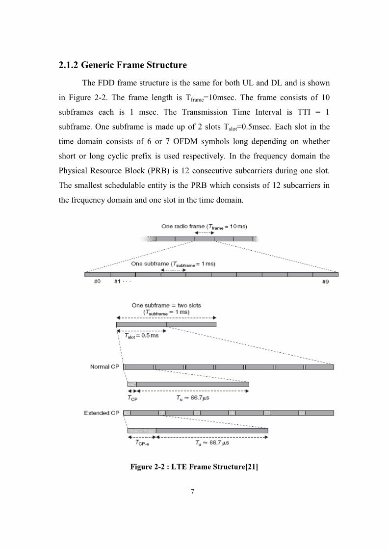
2.1.2 Generic Frame Structure
The FDD frame structure is the same for both UL and DL and is shown
in Figure 2-2. The frame length is Tframe=10msec. The frame consists of 10
subframes each is 1 msec. The Transmission Time Interval is TTI = 1
subframe. One subframe is made up of 2 slots Tslot=0.5msec. Each slot in the
time domain consists of 6 or 7 OFDM symbols long depending on whether
short or long cyclic prefix is used respectively. In the frequency domain the
Physical Resource Block (PRB) is 12 consecutive subcarriers during one slot.
The smallest schedulable entity is the PRB which consists of 12 subcarriers in
the frequency domain and one slot in the time domain.
Figure 2-2 : LTE Frame Structure [21]

8
The scheduling in the uplink is done on a TTI basis, therefore
assignment is carried out in terms of consecutive pairs of PRBs.
2.1.3 Reference Signals
To enable coherent demodulation at the eNB reference signals for
channel estimation are transmitted in the uplink. Uplink reference signals are
time multiplexed with uplink data and therefore are transmitted with the same
transmission bandwidth as the data. As these signals are only transmitted in the
bandwidth assigned to the user they cannot be used to estimate the channel for
the user on the other frequencies not assigned to him. To perform channel
dependant scheduling the eNB need to estimate the channel quality for the user
on the whole bandwidth and to that aim channel-sounding reference signals are
also transmitted. The difference between the channel sounding and
demodulation reference signals are:
1) Channel-sounding reference signals have much larger
transmission bandwidth than demodulation reference signals.
2) Channel-sounding reference signals are transmitted less often
than demodulation reference signals.
3) Channel sounding reference signals from more than one user can
be transmitted within the same frequency band. This is achieved
by sharing the resource in the time domain, frequency domain or
using different cyclic shifts.
The blocks assigned for channel sounding reference signals are not
available for uplink data transmission.

9
2.2 Link Adaptation
Link adaptation is the ability of the system to match the data rate of the
users to the channel conditions for a given transmission power. This is achieved
by Adaptive Modulation and Coding. (AMC) provides two degrees of freedom,
the choice of the modulation scheme and the choice of the coding rate. Higher
order modulation schemes provide high data rates but are more prone to errors
as they are easily affected by variations in interference, noise and errors in
channel estimations. Therefore they should be chosen for high SINR values.
The code rate can be adapted such that a low code rate is chosen for bad
channels.
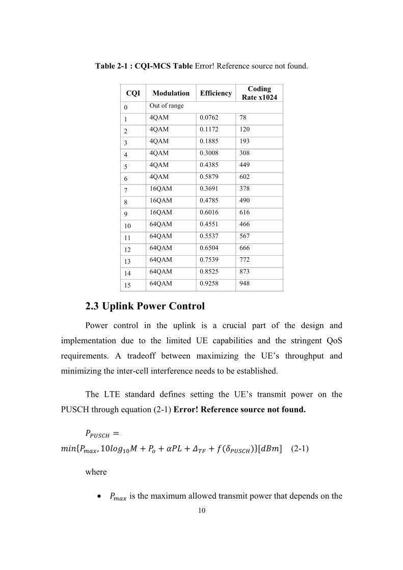
The LTE standard supports AMC by providing different modulation and
coding rates for the different SINR ranges. Table 2-1 is accessed with the
Channel Quality Indicator (CQI) value and the corresponding modulation and
Effective Code Rate (ECR) is achieved. The CQI is mapped from the SINR
value which is calculated from the channel estimation. In the uplink the eNB
estimates the channels from the sounding reference signals.
In the design of the AMC scheme for the LTE one of the issues was
whether to assign the MCS on a per PRB basis or on an assignment basis that is
all PRBs assigned to one user should have the same MCS. Since it was found
that assigning the MCS on a PRB basis only improved the performance slightly
and that the signaling overhead was much higher, the LTE standard specified
that the MCS will be assigned on an assignment basis.
Another issue is the frequency of the AMC decision. Whether the MCS
should be selected every TTI or once every period of time is left to the vendor
implementation.
10
Table 2-1 : CQI-MCS Table Error! Reference source not found.
CQI Modulation Efficiency Coding
Rate x1024
0 Out of range
1 4QAM 0.0762 78
2 4QAM 0.1172 120
3 4QAM 0.1885 193
4 4QAM 0.3008 308
5 4QAM 0.4385 449
6 4QAM 0.5879 602
7 16QAM 0.3691 378
8 16QAM 0.4785 490
9 16QAM 0.6016 616
10 64QAM 0.4551 466
11 64QAM 0.5537 567
12 64QAM 0.6504 666
13 64QAM 0.7539 772
14 64QAM 0.8525 873
15 64QAM 0.9258 948
2.3 Uplink Power Control
Power control in the uplink is a crucial part of the design and
implementation due to the limited UE capabilities and the stringent QoS
requirements. A tradeoff between maximizing the UE’s throughput and
minimizing the inter-cell interference needs to be established.
The LTE standard defines setting the UE’s transmit power on the
PUSCH through equation (2-1) Error! Reference source not found.
{ } (2-1)
where
is the maximum allowed transmit power that depends on the

11
UE power class
M is the number of PRBs assigned to the user in this subframe
is a parameter with a cell specific nominal component and a
UE specific component
referred to as the path loss compensation factor is a 3-bit cell
specific parameter with values {0,0.4,0.5,0.6,0.7,0.8,0.9,1}.
indicates no path loss compensation i.e the power is
adjusted without regards to the user’s pathloss, while
indicates full compensation of the path loss. Values between 0
and 1 indicate partial compensation of the path loss.
is the downlink path loss estimate
is a cell specific parameter function in the Transport Format
(MCS)
is a UE specific value referred to as a Transmitter Power
Control (TPC) command or closed loop correction value. f(*)
can represent an accumulation function or a current absolute
value, the function type is a UE specific parameter.
The equation without the parameter represents open
loop power control, which means that the UE adjusts its power
without intervention from the eNB. The addition of this parameter
converts the equation to closed loop power control where the
eNB can adjust the UE’s power through this parameter.
For further information regarding the power control parameters refer to
the LTE standard [26].
The choice of these parameters affects the power control scheme. Power
control schemes can be categorized based on the value of α. For α=1 this will
lead to full compensation of the path loss, where the transmission power is
increased to compensate for the path loss and the higher the path loss the higher
the transmission power, giving a conventional power control scheme.
12
α=0 will lead to no compensation of the path loss and therefore no power
control. 0<α<1 leads to fractional power control schemes where the path loss is
only partially compensated for.
Another categorization for the power control scheme is whether it is
open loop or closed loop. In open loop power control scheme the UE set its
uplink transmit power based on measurements and estimations done at the UE.
In closed loop power control schemes the eNB can control the uplink transmit
power of the UE. In equation (2-1) the parameters , , and are cell
specific values signaled to the UE by the eNB once. The path loss can be
estimated at the UE and the number of PRBs M is known at the UE. From this
it can be seen that the first part of equation (2-1)
which can be considered as an open loop power control, where the UE
can adjust its power without further signaling from the eNB. The addition of
will make the power control scheme a closed loop one, since the
eNB will signal this parameter to adjust the power of the UE. As can be seen
from the uplink transmit power equation, the closed loop power control is
based on the open loop point of operation, that is the eNB only send correction
values to the open loop power.
2.4 QoS and EPS bearers
Nowadays mobile station applications are not limited to voice. This
wide range of applications introduced different levels of requirements leading
to different QoS classes definitions. While some application could tolerate
relatively high packet delay they could not tolerate high packet loss ratio. To
address the different requirements for the applications different EPS bearers are
established each with a different set of QoS requirements.
The first categorization for the EPS bearers depends on the nature of the
QoS they offer

13
Minimum Guaranteed Bit Rate (GBR) bearers: these have
dedicated transmission resources allocated for the bearer which is
usually done in the admission control functionality of the RRM.
Non-GBR bearers: these do not guarantee a bit rate and therefore
no resources are permanently allocated to the bearer.
Each EPS bearer is also defined with a QoS Class Identifier (QCI) and
an Allocation and Retention Priority (ARP). The parameters associated with
each QCI have been standardized so that uniform traffic handling can be
expected regardless of the eNB vendors’ implementation as shown in Table
2-2. The ARP parameter is used only during bearer establishment i.e. during
admission control only, it governs whether or not the bearer could be accepted
and the priority of the bearer in relation to a new bearer that would be
established. Scheduling decisions are governed by the parameters associated
with the bearer’s QCI. All packets forwarded on the same EPS bearer receive
the same QoS level, therefore to provide a different QoS level a separate EPS
bearer must be established.
Table 2-2 : Standardized QCI for LTE [27]
QCI Resource
Type
Priority Packet
delay (ms)
Packet error
loss rate
Example Services
1 GBR 2 100 10-2
Conversational Voice
2 GBR 4 150 10-3
Conversational video (live
streaming)
3 GBR 5 300 10-6
Non-conversational video
(buffered streaming)
4 GBR 3 50 10-3
Real Time Gaming
5 Non-GBR 1 100 10-6
IMS Signaling

14
QCI Resource
Type
Priority Packet
delay (ms)
Packet error
loss rate
Example Services
6 Non-GBR 7 100 10-3
Voice,video(live streaming),
interactive gaming
7 Non-GBR 6 300 10-6
Video (buffered streaming)
8 Non-GBR 8 300 10-6
TCP-based(e.gWWW,e-
mail)chat,FTP,p2pfile sharing,
progressive video, etc.
9 Non-GBR 9 300 10-6

15
2.5 Reports Sent by UE
2.5.1 Buffer Status Reports
To allocate resources efficiently the uplink scheduler at the eNB needs
to know the requirements of the different UEs in terms of pending data. The
UE informs the eNB of the amount of data in its buffer by means of Buffer
Status Reports (BSR).
EPS bearers are mapped to radio bearers and the radio bearers are
mapped to logical channels. BSR’s are reported on logical Channels.
There are two types of BSRs. A Short BSR which reports the amount of
data available in one logical channel or logical channel group. The Long BSR
reports the amount of data in the buffers of four logical channels or logical
channel groups. The choice of which type of BSR to transmit depends on how
many logical channels have data in their buffers or the amount of available
uplink resources.
When a BSR is triggered and there are not enough resources to transmit
it, a 1 bit Scheduling Request is transmitted or the Random Access procedure is
performed to request uplink resources to transmit the BSR.
2.5.2 Power Headroom Reports
Power Headroom reports are sent by the UE to the eNB to inform the
latter of the amount of available power at the UE. Each UE has a maximum
uplink power transmission limit that it cannot exceed; therefore assigning
resources to a UE which has reached its maximum power limit will be a waste
of resources as the UE will not be able to benefit from the allocation. The eNB
can then use the power headroom report to determine how much more
bandwidth it can allocate to a UE or how much extra bandwidth was previously

16
allocated.
The eNB can also use the power headroom reports to calculate the path
loss of the users from it using the PPUSCH power control equation as shown in
equation (2-2)
PH = Pmax - PPUSCH [dBm] (2-2)
where PH is the Power Headroom
Pmax is the maximum allowed uplink transmission power
PPUSCH is the uplink transmission power

17
Chapter 3
Problem Description and Overview of Related
Work
3.1 Problem Description
The 3GPP LTE standard was put based on a set of requirements and
design targets. To achieve these targets the LTE used new technologies such as
multi-carrier, multiple antennae and packet switched radio interface. As these
technologies help improve system performance they impose new constraints
and challenges for the design and implementation problem.
To exploit the new dimensions of frequency and space introduced by
OFDM and MIMO respectively, cross layer techniques between the physical
layer and the link layers should be implemented. Some of these techniques
which exploit the frequency dimension include channel dependant scheduling,
dynamic link adaptation and power control. It is then noted that optimizing the
RRM functionalities depend on the physical layer configurations.
In addition to the constraints and requirements introduced by the
standard specifications and the technologies used, the RRM design must
consider the requirements and constraints of the different types of applications
or what is known as providing the appropriate QoS to the appropriate traffic
type. Proportional to the importance of this issue is its complexity as more
diverse applications with different requirements are introduced.

18
Time Domain Scheduler
Frequency Domain Scheduler
AMC
Power Control
Channel Estimation and
SINR calculation
SINR to CQI mapping
QoS parameters
BSR
PHR
CQ
I S
INR
S
RS
Tx BW
Allocation
MCS
TPC Commands
Figure 3-1 : The RRM Design Problem Visualization

19
3.1.1 RRM Functionalities
As radio resources are scarce and at the same time the number of users
and their demands increase, managing the radio resources becomes a crucial
point in the performance of any wireless network. The two main resources that
need management are the transmission bandwidth and uplink power. The RRM
functionalities are:
Admission Control: This function ensures that a new user is not
allowed to join the network unless there are enough resources to
meet its QoS requirements. This function is performed only
during EPS bearer establishment.
Scheduling transmission bandwidth: The number of users is
larger than the available bandwidth. The scheduler function is to
determine each TTI, which users to be served, the transmission
bandwidth allocated to each user and the location of this
bandwidth in the spectrum.
Link Adaptation: The link adaptation determines the transport
format of the packets for each user, i.e. it assigns a modulation
and coding scheme. It also performs power control to have the
users operate at a target SINR.
3.1.2 RRM Constraints and Challenges
The implementation of the above RRM functionalities must meet the
requirements of the system and users while respecting the constraints of the
technologies.
The constraints on the scheduler can be summarized as (1) the number
of available PRBs, (2) for each PRB at most one user can be assigned. For the
link adaptation functionality the constraints are (1) the available

20
modulation schemes, (2) the available code rates, (3) the maximum
transmission power.
SC-FDMA was chosen as the uplink transmission scheme for LTE. This
adds a constraint on the scheduler functionality that the PRBs allocated to one
user must be contiguous in frequency.
Figure 3-2 : Contiguous Assignment of PRBs in SC-FDMA
The main requirements the RRM functionalities must meet are those
related to the QoS parameters. The RRM functionalities should provide each
user with the QoS the connection was established based on. This includes
meeting the guaranteed bit rate, maximum tolerated packet delay and maximum
tolerated packet loss ratio.
Besides the constraints and requirements the RRM functionalities must
address the issues of system performance. Design of RRM algorithms should
consider issues such as maximizing spectral efficiency and overall system

21
throughput, minimizing inter-cell interference and providing fairness among
users.
3.1.3 Inputs to the RRM
To serve its purpose the RRM is provided with inputs to help it take
informed decisions.
The channel conditions which are required for the link adaptation and
scheduling can be estimated for the whole bandwidth for each user with the
help of the channel sounding reference signals. The SINR is calculated for the
SRS’s and then mapped to a CQI. For the downlink the UE sends CSI reports
to the eNB.
To distinguish active users with data in their buffers from idle users,
each user with data pending in its buffers sends a one bit Scheduling Request
(SR) to the eNB informing it with the need for UL grants.
The information about the amount of data available at each user’s
buffers is collected by means of buffer status reports.
The UE sends Power Headroom Reports to the eNB to inform it about
the amount of available power the UE has which is used in the power control
and scheduling functionalities of the RRM. The PHR can also be used to
estimate the downlink path loss.

22
UE eNB
Buffer 1
Buffer 2
Buffer 3
Buffer 4
SR
BSR
PHR
SRS
UL Grant
MCS
TPC
RRM
Figure 3-3 : UE-eNB Signalling

23
3.2 Related Work
3.2.1 Channel Dependant Scheduling
Frequency Domain Packet Scheduling also known as Channel
Dependant Scheduling exploits the multiuser diversity to increase spectral
efficiency and throughput. The idea behind channel dependant scheduling is
that not all users see the channels in the same way. A channel which one user
has very low gain on, can have very high gain for another user as seen in Figure
3-4 [21]. The scheduling decision is the assignment of resource blocks to users
in such a way as to maximize a utility function based on throughput. The
channels for each user are obtained by providing the SRS to a channel
estimation algorithm. To simplify the problem and focus on the scheduling part
of it, perfect channel knowledge is assumed in the majority of the literature
addressing this problem.
Figure 3-4 : Channel Dependant Scheduling [21]
3.2.1.1 Heuristic Algorithms for Channel Dependant Scheduling
The following work tackled the channel dependant scheduling from a
heuristic point of view to decrease computational complexity and provide a

24
cost efficient implementation.
S. Lee et al. in [1] evolved the conventional Round Robin algorithm and
introduced four algorithms to address the problem of uplink scheduling in the
LTE.
Algorithm 1: Carrier by Carrier in turn. Round robin on the RBs
starting from RB number 1, the RB is assigned to the user with
the highest Proportional Fair (PF) metric
⁄ ,
on the RB without violating the contiguity constraint, where r is
the instantaneous channel rate for user i on RB c at time t, and R
is the long term average rate of user i.
Algorithm 2: Largest Metric Value RB First. Same as algorithm 1
but instead of starting with RB number 1 start with the RB with
the highest metric value, if 2 non-adjacent RBs are assigned to
the same user, the RBs in-between these 2 assigned RBs are also
assigned to the same user.
Algorithm 3: Riding Peaks. The idea is based on that there is
correlation between adjacent RBs i.e. if for a user a certain RB
has high metric it is with high probability that the neighboring
RBs will also have high metrics. Same as algorithm 2 look at the
highest metric value RB first, the RB is assigned to user i if the
RB is adjacent to the previously assigned RBs of user i or user i
has no RBs assigned yet. Otherwise it is not allocated and we
move on to the next RB.
Algorithm 4: RB Grouping. Algorithm 3 is expected to yield
good results if the frequency domain exhibits high correlation
between two adjacent RBs. However correlation in the frequency

25
domain is not strong which implies that even though we have an
overall frequency correlation the granularity of this correlation is
not necessarily as small as one RB. To deal with this issue of
small scale variations the unit of consideration will be RB group.
A RB group is a number of contiguous RBs viewed as one block
together.
In [2] a Search-Tree Based packet scheduling algorithm is proposed.
The idea is to draw a binary tree where each node has 2 branches the maximum
utility and the second maximum utility. Allocation is decided at the end where
the path with the highest overall global utility is chosen. In the simulations the
bandwidth is assumed equal and fixed for all UEs therefore neglecting the
adaptive transmission bandwidth problem, imperfect channel knowledge is
considered through considering HARQ retransmissions, and open loop power
control is implemented.
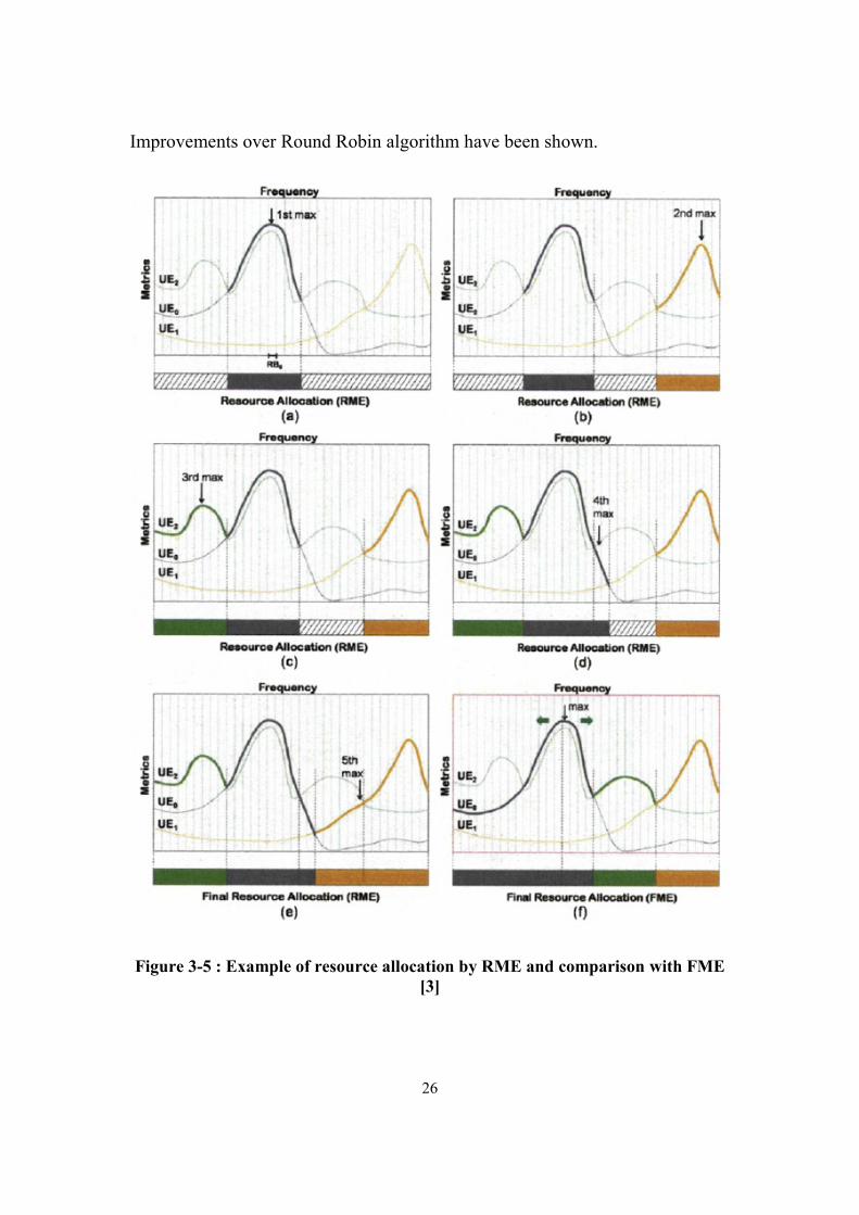
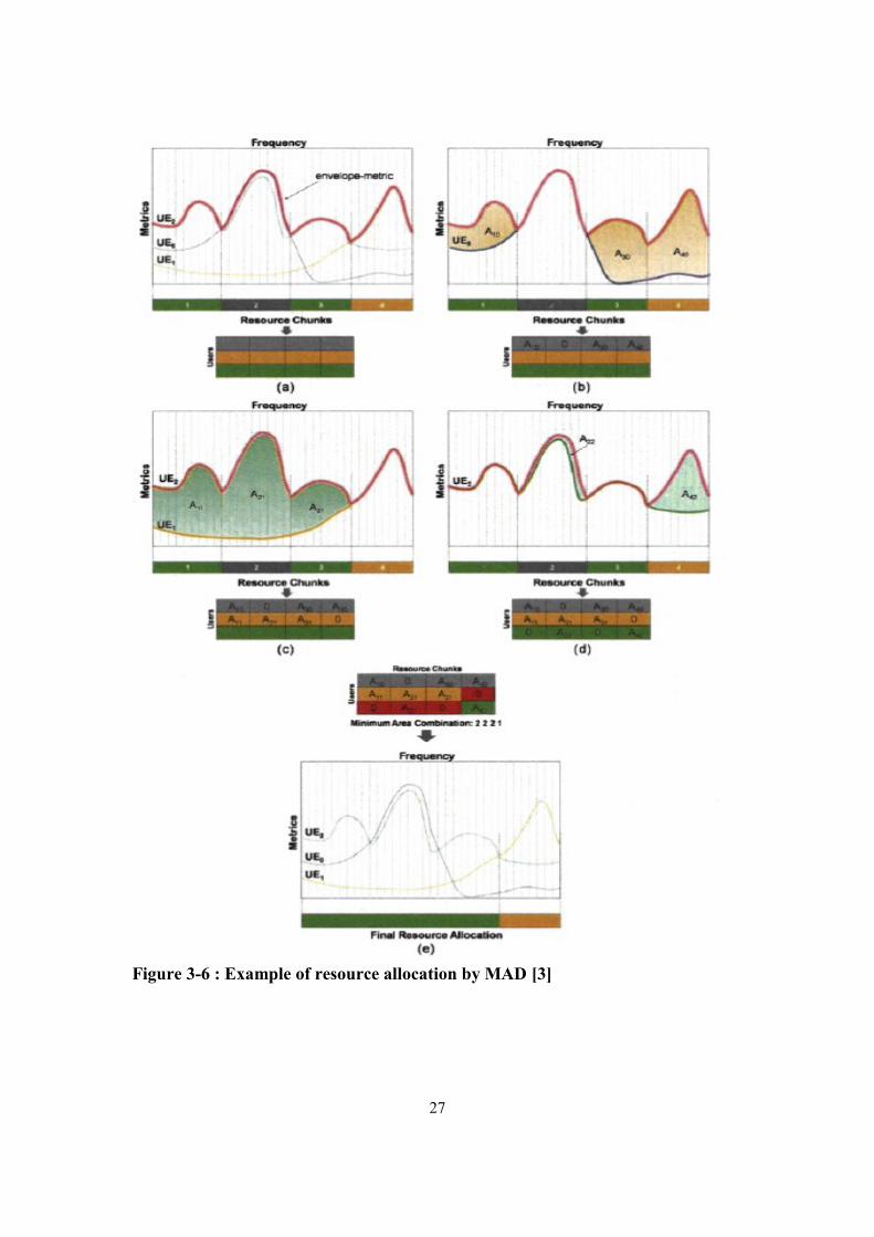
In [3] three heuristic algorithms were proposed. First Maximum
Expansion (FME) algorithm assigns resources starting from the highest metric
value and expanding the allocation on both sides, the allocation for a UE is
stopped whenever another UE with a higher metric is found. The second
algorithm Recursive Maximum Expansion (RME) is similar to the first one
except that it performs a recursive search of the maximum. Figure 3-5 shows a
comparison between the allocation done using RME and FME. Minimum Area
Difference (MAD) to the Envelope algorithm’s scope is to derive the resource
allocation that provides the minimum difference between its cumulative metric
and the envelope-metric, i.e., the envelope of the users' metrics. An example of
how the resources are assigned is shown in Figure 3-6. Although MAD is a
more computationally expensive algorithm than the previous two however it
gives closer results to the optimal solution. This algorithm aims at minimizing
the difference between its cumulative metric and the envelope metric.
26
Improvements over Round Robin algorithm have been shown.
Figure 3-5 : Example of resource allocation by RME and comparison with FME
[3]
27
Figure 3-6 : Example of resource allocation by MAD [3]

28
In [4] the authors combine the work of [2] and [3] and propose two
improvements for the Recursive Maximum Expansion Algorithm. The first
algorithm gives higher flexibility in the RB expansion by not limiting the
expansion only to the maximum but having it to be within a threshold, while
the second algorithm Improved Tree Based Recursive Maximum Expansion
gives even more flexibility in the expansion by considering the highest and
second highest metric deriving a binary search tree. Results show that with a
little higher complexity around 15% gain in spectral efficiency is obtained
compared with conventional Recursive Maximum Expansion.
The authors in [5] looked at the problem from a different view by
focusing on investigating different scheduling metrics, mainly a combination of
two metrics throughput based in the time domain and SINR based in the
frequency domain. Scheduling metrics affect the priority of the users.
Evaluations are based on a RRM framework with open loop power control and
AMC.
A Heuristic Localized Gradient Algorithm (HLGA) is discussed in [6].
The algorithm simplifies the optimal Localized Gradient Algorithm (LGA) by
following a simple heuristic in allocating the RBs to the users while
maintaining the required allocation constraint and taking retransmission
requests into consideration. The basic idea is to search for the RB-user pair
with the highest metric value and assigning this RB to this user, if the user has
previous allocations that is not contiguous to the new allocation, all in-between
RBs are assigned to the user. The HLGA is compared to a reference algorithm
LGA which defines and solves an optimization problem. In [7] the authors
examined the performance of the HLGA when dynamic traffic models are
assumed. To solve the problem of different buffer occupancies and therefore
different users' requirements, a procedure called 'pruning' is introduced. The
pruning procedure states that RBs are first assigned to users according to the
29
HLGA regardless of their traffic requirement. Extra RBs allocated to users are
then reallocated to either neighboring users in the spectrum or users with no
assignments. Pruning is performed on edge RBs to preserve the contiguity
constraint.
3.2.1.2 Optimization Problem of Channel Dependant Scheduling
The channel dependant scheduling problem was addressed as an
optimization problem to obtain an optimal solution. As these solutions usually
need high computation resources they are mostly used as a benchmark and
reference for other suboptimal or heuristic solutions. In [6] and [8], the authors
discussed the optimization problem and provided suboptimal algorithms to
solve it.
In [6] the gradient metric was chosen as the scheduling metric for the
scheme. The utility function is a strictly concave smooth utility function. An
integer programming assignment problem is formulated with a contiguity
constraint. The integer programming optimal solution assumes perfect channel
knowledge, in case of measurement delays and estimation errors, the selection
rule occasionally picks rates that do not match the channel capacity.
Synchronous non adaptive HARQ is assumed to take care of these errors and
therefore a constraint is added to allocate to the users having HARQ processes
operating on certain RBs those same RBs until successful transmission is
achieved. In this case the solution provided is not the optimal one.
In [8] a general LTE UL Frequency Domain Packet Scheduling (FDPS)
problem is formulated. The problem defines a profit function which is a general
term used to represent various scheduling policies. The aim is to schedule the
RBs in a time slot such that the profit is maximized. The LTE UL FDPS
problem is shown to be NP-hard and therefore two approximation algorithms
are introduced which computes solutions close to the optimum. The first

30
heuristic algorithm is a greedy strategy based algorithm which divides the LTE
UL FDPS problem into several sub problems according to the profit and then
apply a greedy method to each problem. The second algorithm is based on a
local ratio technique.
The aforementioned algorithms have all assumed full buffer traffic
model, fixed traffic classes and only focusing on increasing overall throughput
with no regards to interference on other cells.
3.2.2 QoS Oriented Scheduling
QoS oriented scheduling considers in addition to increasing throughput,
per-flow metrics such as packet loss and packet delay. In today’s wireless
networks, more diverse applications, such as video and interactive gaming, are
introduced leading to different QoS requirements. The scheduling scheme
should consider these variations when assigning resources. QoS parameters
including maximum allowed packet delay, maximum allowed packet drop
ratio, priority and guaranteed bit rate GBR must be respected. In the channel
dependant scheduling problem, the utility function is usually a function of the
overall rate is to be maximized under the contiguity constraint. When QoS
classes are accounted for in the resource assignment, this will add further
constraints on the scheduler.
3.2.2.1 Downlink QoS Oriented Scheduling
The following papers discussed QoS-oriented scheduling but from the
downlink point of view. Downlink scheduling is a simpler problem than the
uplink as the contiguity constraint is removed. Another issue that is different in
the downlink from the uplink is that the HOL packet delay in the downlink is
available at the eNB while in the uplink it is either estimated or the buffer
status is used instead.
The authors in [9] expanded the channel dependant scheduling

31
problem to include buffer status awareness. AMC is also implemented where,
the MCS is chosen depending on the CQI reported by the UE. Proportional
fairness is achieved by preferring users with good channel conditions to be
scheduled but at the same time if the user is scheduled frequently the priority of
the user is decreased. A priority function is proposed to achieve four objectives
1) maximize system throughput 2) decrease packet drop ratio 3) keep certain
fairness among users 4) guarantee QoS of multimedia services. The priority is a
function of the buffer status, the instantaneous data rate, the average data rate,
priority of the service class and GBR for RT services. For each subband the
priority function is calculated for all the users and the subband is allocated to
the user with the highest priority on this subband.
In [10] a decoupled time and frequency domain scheduler is proposed.
The time domain scheduler helps in reducing the complexity of the frequency
domain scheduler by minimizing the set of schedulable users. Users are added
to the set of schedulable users if they satisfy that they have data to be
transmitted and that the data has passed either the buffer amount threshold or
the head of line threshold. The schedulable users are then prioritized according
to a set target bit rate. The frequency domain scheduler then selects for PRB k
the user n that maximizes a chosen metric. Three metrics are investigated
Proportional Fair:
where is the past average throughput of user n
is the estimated achievable throughput for user n on PRB k
Proportional Fair Scheduled:
where is an estimate of the user throughput if user n was
scheduled every sub-frame.
32
Carrier Over Interference to Average.
∑
where is an estimation of the SINR on the kth
PRB of the nth
user. The denominator describes the average channel quality of the user.
In [11] the authors propose a delay prioritized scheduling algorithm
consisting of three steps. Step 1 the algorithm computes for each user the
remaining time of the HOL packet delay to approach the delay threshold. Step
2 the user with the lowest difference between the HOL delay and the threshold
is chosen. Step 3 finds the RB with the highest gain for the selected user and
assigns the RB to it.
In [12] a similar approach is adopted where the users are classified into
three categories according to their HOL packet delay and then the packet
scheduler allocates RBs to corresponding users according to their priorities.
3.2.2.2 Uplink QoS Oriented Scheduling
The QoS oriented scheduling was discussed in the uplink in the
following papers.
In [13] two algorithms are proposed which consider the end to end
packet delay constraint in addition to the contiguity constraint imposed in LTE
uplink scheduling. The first algorithm goes through each RB and assigns it to a
user taking into account the contiguity constraint if the maximum delay and
minimum throughput requirements are satisfied for all the users. Otherwise it
assigns first the users with critical delay or throughput as long as RBs are
available and do not violate the contiguity constraint. The second algorithm
differs from the first one in the use of a different metric value and that RBs are
not assigned in order but with respect to users with critical delay requirement.
Both algorithms tend to assign one block per user and therefore are not

33
efficient in the case when the number of users is smaller than the number of
RBs, also in both algorithms some users may never be assigned RBs.
In [14] the constraint of the queuing delay is studied under the goal to
minimize power transmission. An optimization problem is formulated and a
suboptimal algorithm is proposed and evaluated.
3.2.3 Uplink Power Control and Interference Coordination
The problem of power control is closely associated with inter-cell
interference. An optimum transmission power is the power that can maximize
system throughput. System throughput is a function of the cell throughput and
the inter-cell interference. The higher the transmission power the higher the cell
throughput but also the higher the inter-cell interference and subsequently the
inter-cell interference decrease the throughput for the neighboring cells. So
basically power control objective is to achieve a transmission power that
maximizes user and cell throughput but at a reasonable inter-cell interference
level. The argument for this concept is that if all eNB’s control the level of
interference they cause to neighboring cells, then each individual eNB will also
receive limited interference from its neighbors resulting in an overall good
performance. This behavior is desirable as it is in synchrony with the concept
of self-organization (SoN) that is being promoted by 3GPP and other forums to
enhance the configuration, optimization, and operations of future wireless
networks [22] [23].
The LTE uplink power control mechanism constitutes of a closed loop
component operating around an open loop point of operation. The open loop
component is derived based on a parameterized power control scheme.
Conventional power control schemes assume full compensation for the path
loss where all users are received with the same SINR, which means that the
higher the path loss the higher the transmission power. Since the path loss to

34
the serving eNB is inversely proportional to the path loss to the neighboring
eNB’s, the conventional power control scheme with full compensation could
lead to high inter-cell interference levels. The uplink power equation as stated
in the 3GPP LTE standard allows the use of Fractional Power Control (FPC)
where users with higher path loss operate at a lower SINR requirement. To
further improve the performance in terms of interference a closed loop
component is added to the open loop. The closed loop component is left to the
implementation of the vendor where usually it is associated with a SINR or
interference target.
While the open loop term determines the tradeoff between cell capacity
and cell outage by compensating for slow variations, the closed loop term
affect the long term performance tradeoff between inter-cell interference and
system throughput by compensating for fast variations.
3.2.3.1 Performance Evaluation of the LTE Uplink Power Control mechanism
In [15] and [16] the authors have evaluated the performance of the
uplink power control mechanism defined in the LTE standard.
The authors in [15] evaluate the FPC equation and study the effect of the
different parameters on the interference levels and the SINR which gives an
indication on the throughput. The paper’s focus was only on the open loop
power control therefore depending on the aim of the PC scheme whether it is to
increase capacity or to improve outage performance, a choice for the different
parameters of the open loop power control equation was made to achieve that.
While authors in [15] focused on the open loop performance, authors in
[16] evaluated the performance of both the open loop and closed loop power
control mechanisms. Investigations of the different parameter sets to give (a)
high bit rate and (b) high capacity have been done.

35
3.2.3.2 Uplink Power Control and ICIC
The following work studied the uplink power control problem and
proposed power control techniques but neglected the effect of some RRM
functionalities.
In [17] the author designed and implemented a closed loop power
control scheme in combination with the fractional path loss compensation
factor. An investigation for the different values of the path loss compensation
factor has been provided as well as a choice for the optimal value that gives
best cell edge and mean user throughput. The SINR Target is set by the eNB as
the target SINR that a UE should be using. The SINR Target affects two
parameters, the throughput and the interference. A mathematical model for
setting the SINR Target based on the path loss is described. The proposed
model assigns a higher SINR Target for users with low path loss therefore
allowing these users to transmit at a higher power. Implementing this model
will decrease the inter-cell interference but at the expense of lower throughput
for the cell edge users.
In [18] the author studied the open loop power control and introduced
two closed loop power control algorithms to enhance the performance.
The first algorithm is designed to set the transmission power
spectral density according to the tradeoff between the UE’s
generated signal and interference powers to achieve a higher
SINR for this UE. The algorithm calculates the total interference
generated by a UE and compares it to an interference limit. While
the interference spectral density limit is equal to all users the
interference limit is dependent on the allocated bandwidth to the
users, but the author assumes equal bandwidth allocation to all
users in the simulation. The transmitting power spectral density is

36
set using the interference spectral density limit.
o A further modification is introduced by adding a factor
similar to the path loss compensation, to tune the path loss
of the UE to the neighboring eNBs. The two path loss
terms (path loss between UE and serving eNB, and path
loss between UE and neighboring eNBs) with their
compensation factors are combined in a formula to obtain
the transmitting power spectral density.
The second algorithm is designed to set the transmission power
according to a throughput measure. While a user may represent a
better tradeoff between signal and interference powers, it is not
necessary to represent a better tradeoff between gain in
throughput and interference. For each user two parameters are
calculated, the gain to the system calculated as the increase in
throughput due to the increase in power, and the cost to the
system calculated as the increase in interference due to the
increase in power. To calculate the increase in throughput an
estimate of the interference this user is experiencing is estimated.
An “interference budget” of the cell is managed by allowing
iteratively one UE to increase its transmission power by one step
until the target interference is met. The UE will be chosen based
on the gain/cost criteria.
In [19] an uplink radio resource management scheme is proposed with
an emphasis on admission control, packet scheduling and handover. The
admission control algorithm is based on fractional power control. The
admission decision for a new user is based on the availability of enough PRBs
to satisfy his QoS requirements. To calculate the number of PRBs required to

37
fulfill the requested GBR, the open loop fractional power control equation is
used. The number of required PRBs of existing users is obtained by using the
average number of PRBs allocated to these users by the packet scheduler.
The admission control algorithm is then combined with a packet
scheduler. The packet scheduling is done in two phases: Time Domain and
Frequency Domain. The time domain scheduler prioritizes the users according
to their GBR requirements giving higher priority to the user further below his
GBR and then selects N users to input to the frequency domain scheduler. The
frequency domain scheduler allocates flexible number of PRBs to the users by
using an adaptive transmission bandwidth based scheduling which aims at
maximizing the sum of a frequency domain metric. QoS is included in the
frequency domain by weighting the frequency domain metric according to the
QoS requirements. The combined admission control and packet scheduling is
evaluated for different traffic profiles.
The work also discusses handover procedure which is out of scope of
this thesis.
38
3.3 Shortcomings of Previous Work
As seen from the previous chapter the LTE uplink RRM problem has
been the interest of many researchers. As the RRM problem is a broad subject
and even though many findings and contributions have been made there still
room for more contributions and improvements.
Previous work when studying the RRM problem mainly focused on one
or two functionalities only. Authors would focus on optimizing the frequency
domain scheduler, or the AMC or the power control functionality. As this
approach optimizes this functionality the effect of the algorithm on the other
functionalities is not studied. Therefore an algorithm optimizing the frequency
domain packet scheduling for example may not be the optimum one from the
point of view of power control and ICIC.
Most previous work also evaluates performance assuming full buffer
model and unified traffic model for all the users. Since this evaluation
disregards the QoS requirements, the performance of the algorithms in terms of
user satisfaction could not be measured. Therefore while an algorithm could
yield high performance metrics in terms of throughput, it can possibly give
very low metrics with respect to respecting the QoS requirements.
39
Chapter 4
The Proposed Radio Resource Management
Framework
4.1 General Framework
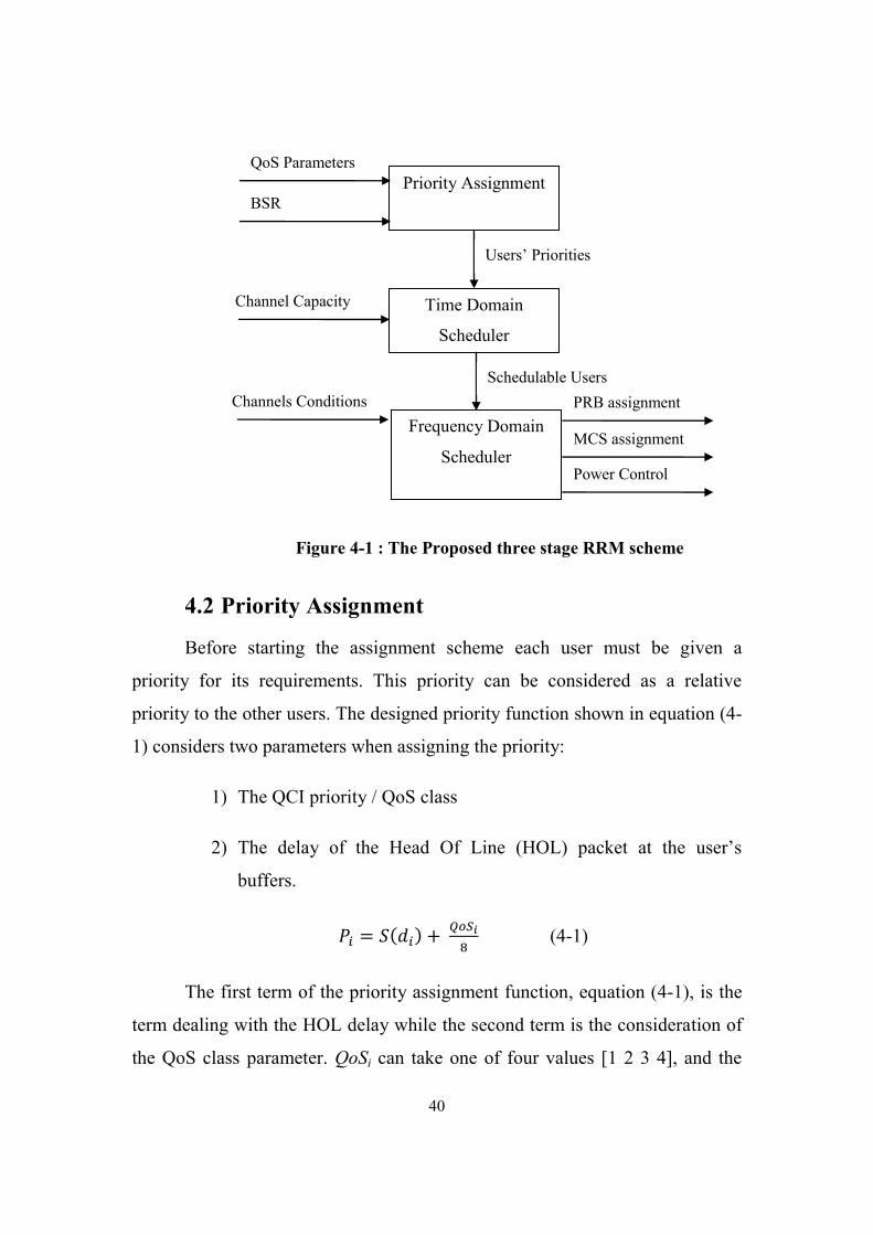
The proposed RRM scheme selects the users to be served in each TTI
from the set of active users and assigns the transmission bandwidth, MCS and
power for the selected users.
The scheme consists of three stages
1) Priority Assignment: In this stage a relative priority is assigned to
each user. This priority is used in the next two stages to decide
whether the user will be served in this TTI or not and how many
resources will be allocated to it.
2) Time Domain Scheduling: To decrease the complexity of the
frequency domain scheduler so as to search in a limited number
of users for the optimum solution, the Time Domain Scheduler
selects from the set of active users according to the priority the
users to be served in this TTI.
3) Frequency Domain Scheduling: The frequency domain scheduler
for each user decides the number and location of PRBs to be
assigned, the MCS and the closed loop power adjustment.
40
4.2 Priority Assignment
Before starting the assignment scheme each user must be given a
priority for its requirements. This priority can be considered as a relative
priority to the other users. The designed priority function shown in equation (4-
1) considers two parameters when assigning the priority:
1) The QCI priority / QoS class
2) The delay of the Head Of Line (HOL) packet at the user’s
buffers.
(4-1)
The first term of the priority assignment function, equation (4-1), is the
term dealing with the HOL delay while the second term is the consideration of
the QoS class parameter. QoSi can take one of four values [1 2 3 4], and the
Priority Assignment
Time Domain
Scheduler
Frequency Domain
Scheduler
QoS Parameters
BSR
Users’ Priorities
Channel Capacity
Channels Conditions
Schedulable Users
PRB assignment
MCS assignment
Power Control
Figure 4-1 : The Proposed three stage RRM scheme

41
function S has values less than one, therefore to have the QoS term comparable
to the delay term and not to have the QoS dominate the priority, the QoS is
divided by 8. di is the average delay of the HOL packet for user i, and S(x) is a
sigmoid function. The sigmoid function was chosen as the function type to only
give weight to the HOL delay when it approaches its maximum allowed value,
as the HOL delay is still small compared to the maximum allowed the main
weight of the priority function will be the QoS class. This way the QoS
requirements are respected and at the same time possible starvation of some
low QoS class users is avoided. The function S [28] is given by:
(4-2)
where is the maximum allowed delay for user i and qi as defined by
equation (4-3) [28], is a quantization constant which indicates the emergency of
the traffic of user i according to its required PELR.
(4-3)
Referring to Table 2-2 we find that the minimum PELR is 10-6
accordingly we set the Total Number of Levels in the system to be equal 6. The
level number is the exponent of the PELR, e.g. for VoIP the maximum allowed
PELR is 10-2
therefore a user with a VoIP traffic shall have a Level number =
2.
The HOL delay is not signaled explicitly to the eNB instead the user
only signals the number of bits in its buffers using BSRs, therefore to have a
realistic implementation; we deduced an approximation equation for the HOL
using BSR.
(4-4)
42
where bi is the amount of data in bits available in the buffers of user i,
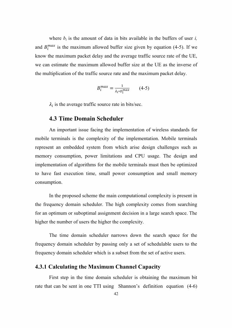
and is the maximum allowed buffer size given by equation (4-5). If we
know the maximum packet delay and the average traffic source rate of the UE,
we can estimate the maximum allowed buffer size at the UE as the inverse of
the multiplication of the traffic source rate and the maximum packet delay.
(4-5)
is the average traffic source rate in bits/sec.
4.3 Time Domain Scheduler
An important issue facing the implementation of wireless standards for
mobile terminals is the complexity of the implementation. Mobile terminals
represent an embedded system from which arise design challenges such as
memory consumption, power limitations and CPU usage. The design and
implementation of algorithms for the mobile terminals must then be optimized
to have fast execution time, small power consumption and small memory
consumption.
In the proposed scheme the main computational complexity is present in
the frequency domain scheduler. The high complexity comes from searching
for an optimum or suboptimal assignment decision in a large search space. The
higher the number of users the higher the complexity.
The time domain scheduler narrows down the search space for the
frequency domain scheduler by passing only a set of schedulable users to the
frequency domain scheduler which is a subset from the set of active users.
4.3.1 Calculating the Maximum Channel Capacity
First step in the time domain scheduler is obtaining the maximum bit
rate that can be sent in one TTI using Shannon’s definition equation (4-6)

43
for the maximum capacity of a communication channel.
(4-6)
where C is the maximum channel capacity in bits/second, B is the
channel’s bandwidth, S is the total received signal power and N is the total
noise power. S/N is also referred to as the signal to noise ratio.
Although there are variations of the SNR from one user to another and
even for the same user from one part of the bandwidth to another, to calculate
the maximum capacity we assume the best channel conditions. By this we
assume that the SNR value is the highest possible which will give the
maximum CQI index.
The number of bits that can be transmitted per PRB in one TTI is
calculated using equation (4-7),
(4-7)
where is the number of subcarriers per PRB, is the number of symbols
per slot, is the number of slots per TTI, and ECR is the Effective Code
Rate (ECR) which is equal to the efficiency obtained from Table 2-1.
To calculate the maximum number of bits that can be transmitted in one
TTI, we assume the best channel conditions and from Table 2-1for CQI=15 we
obtain the highest possible modulation scheme and coding rate which is
64QAM i.e. 6 symbols per slot, and ECR = 0.9258.
4.3.2 Selection Criteria
The normal case scenario in any wireless network is that the requests of
the active users exceed the maximum capacity of the channel. The basic idea of
the time domain scheduler is to select from the set of active users the users that

44
will be served in this TTI.
Users are sorted in a descending order of priority. As mentioned in the
previous section the priority is a function of QoS requirements and buffer
queue size. Users are scheduled in this TTI as long as the cumulative
throughput request did not exceed the maximum capacity.
It is possible that users may have equal priority. When sorting these
users the user with the worse channel conditions is given higher priority than
the user with better channel conditions. This is done to improve the users’
chance of finding a good enough channel to transmit on. The time domain
scheduler is depicted in Figure 4-2.
4.4 Frequency Domain Scheduler
The frequency domain scheduler assigns the transmission bandwidth to
the users selected by the time domain scheduler. In addition to the transmission
bandwidth the frequency domain scheduler is also responsible for assigning the
MCS and adjusting the uplink power.
In short the time domain scheduler is responsible for selecting the users
1. Find the set of active users (users with traffic in their buffers)
2. Sort the active users according to their priority as assigned by the priority function.
3. In case more than one user have the same priority, sort the equal priority users such
that the worst channel gets served first.
4. Calculate the maximum capacity of the system.
5. The first group of users whose scheduling request fills the maximum capacity is
chosen to be served in this TTI.
Figure 4-2 : Time Domain Scheduler

45
to be served in this TTI and the frequency domain scheduler is responsible for
selecting and assigning the resources to these users.
The users are passed to the frequency domain scheduler sorted by their
priorities. The frequency domain scheduler serves the users one at a time
starting with the highest priority user. Each user is served until the user’s
request is satisfied or the resources are consumed.
Due to the fact that there is a high correlation in the frequency domain
between the adjacent PRBs, this means that a PRB adjacent to a PRB with high
gain will probably have high gain as well. From this the PRB assignment is
done starting with the PRB with the highest gain and then assigning PRBs left
and right of the maximum gain PRB. This should help reduce the number of
PRBs needed to satisfy the user’s request.
1. Let U be the set of users to be served
2. Let A[i] be the allocation matrix, i is the PRB index. The value of A[i] is the
user index assigned to the PRB.
3. Initialize A to be zeros indicating PRB is empty
4. Define PRB_Groupk as a set of empty contiguous RBs in A
5. for User = 1 to number of users do 6. Get all available PRB_Groups in A
7. for k = 1 to number of available PRB_Groups do
a. Calculate this user’s average gain on PRB_Groupk
b. Get maximum power allowed to the user set by the system
c. Estimate the user’s overall request from the BSR
d. Obtain the MCS from the power and calculate the average number of
PRBs needed to satisfy the user request, the minimum of the
calculated number of PRBs and the number of PRBs in the
PRB_Group is taken.
e. Calculate the closed loop power adjustment (TPC)
f. Calculate the PUSCHP using the outputs of steps d and e.
g. Recalculate the needed number of PRBs and the MCS using the
calculated transmission power in step f.
h. Find the PRB with the maximum gain in the PRB_Group.
i. Assign the peak PRB to the user.
j. Assign the PRBs left and right of the peak until the calculated number
of PRBs is assigned.
8. end for
9. Find the PRB_Group that gives the highest number of bits to the user with the
minimum number of PRBs
10. Assign this PRB_Group to this user, update A[i]=user_id for assigned PRBs
11. end for
Figure 4-3 : Frequency Domain Scheduler

46
For each user the frequency domain scheduler finds the set of
schedulable groups of contiguous PRBs. For each PRB group the number of
bits that the user can send on this group is calculated. The PRB group which
satisfy the user’s request in the minimum number of PRBs or the PRB group
which gives the user the highest number of bits that can be sent, is assigned to
this user. This is repeated until all the users are served or all the bandwidth is
assigned.
4.5 SINR-CQI Mapping and AMC
To perform AMC the scheduler at the eNB needs to know the channel
conditions for each user, such that the appropriate modulation scheme and
coding rate is assigned. The channel conditions are estimated from the received
uplink SRS. The channel estimation from the SRS is outside the scope of this
thesis and therefore perfect channel knowledge is assumed.
The next step is to calculate the Signal to Noise Ratio (SNR) for the
channel as in equation (4-8). It is more accurate to calculate the Signal to
Interference and Noise Ratio (SINR) instead of the SNR, but we neglect
interference power for simplicity without loss of generality.
(4-8)
where is the received signal power, is the total noise power, and NF
is the noise figure at the receiver.
Since this is a fading channel the SNR is not used directly as is to obtain
the channel CQI. An effective SNR is used instead to take the effect of the
channel gain and path loss into consideration.
| |
(4-9)
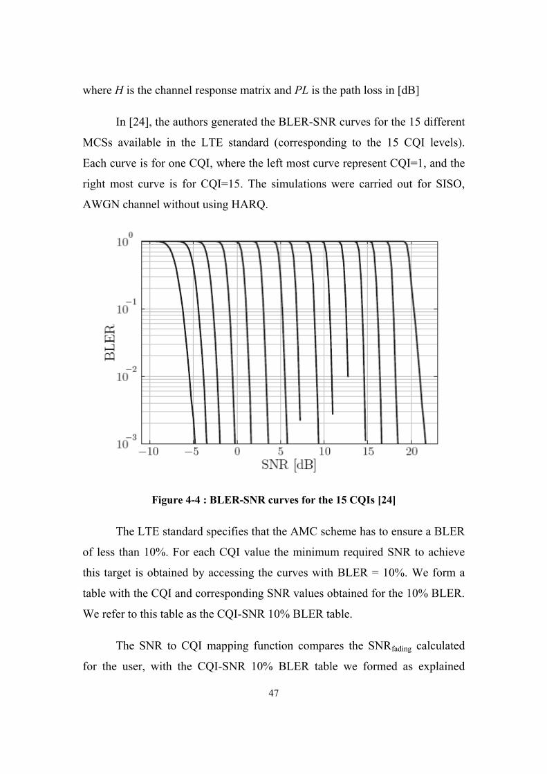
47
where H is the channel response matrix and PL is the path loss in [dB]
In [24], the authors generated the BLER-SNR curves for the 15 different
MCSs available in the LTE standard (corresponding to the 15 CQI levels).
Each curve is for one CQI, where the left most curve represent CQI=1, and the
right most curve is for CQI=15. The simulations were carried out for SISO,
AWGN channel without using HARQ.
Figure 4-4 : BLER-SNR curves for the 15 CQIs [24]
The LTE standard specifies that the AMC scheme has to ensure a BLER
of less than 10%. For each CQI value the minimum required SNR to achieve
this target is obtained by accessing the curves with BLER = 10%. We form a
table with the CQI and corresponding SNR values obtained for the 10% BLER.
We refer to this table as the CQI-SNR 10% BLER table.
The SNR to CQI mapping function compares the SNRfading calculated
for the user, with the CQI-SNR 10% BLER table we formed as explained

48
above. The CQI of the first SNR value that is less than or equal to the SNRfading
is chosen for the user. The CQI is then used to access the CQI-MCS table to
obtain the modulation scheme and coding rate to be assigned.

49
4.6 Closed Loop Power Control and ICIC
At first glance a tradeoff between increasing cell throughput and
decreasing the generated interference on neighboring cells exist. Deeper
analysis shows that if the overall system inter-cell interference decreased, this
will provide higher system throughput due to decreasing erroneous
transmissions and therefore decreasing retransmissions.
Still the scheduler is faced with the design challenge of maximizing the
throughput while minimizing the generated interference which are two
conflicting goals as maximizing throughput requires the use of high
transmission power while minimizing interference requires the use of lower
transmission power. Therefore a balance between the two should be found.
Previous work considered each issue separately, frequency domain
scheduling aiming at maximizing throughput has been studied before as well as
power control techniques to minimize inter-cell interference, but these studies
did not consider the mutual effect these issues have on each other. Therefore
the algorithms maximizing throughput did not analyze the effect on inter-cell
interference and the algorithms minimizing interference did not consider
maximizing the throughput.
In this thesis we present a closed loop power control mechanism that is
an integrated part of the resource management framework. The mechanism
considers the tradeoff between maximizing throughput and minimizing inter-
cell interference and the effect of each requirement on the other is analyzed.
The mechanism is based on the LTE closed loop power control equation
(2-1) which is explained in chapter 2.3
{ }

50
The main goal of the algorithm is setting such that
interference is minimized and throughput is maximized. As can be seen from
the above equation the power equation is also dependant on M the number of
PRBs assigned to the user. Previous work studying ICIC mostly assumed M as
a fixed number known from the beginning usually by equally dividing the
bandwidth among the users.
The power control mechanism is presented here as a part of an
integrated radio resource management framework assigning both M and
to meet both the requirements of system efficiency and ICIC.
Contrary to previous work where power control mechanisms are applied after
the frequency domain scheduling, in our work power control and frequency
domain scheduling are done simultaneously in the frequency domain scheduler.
The ICIC algorithm is done as a 2 step process:
Step 1a: Using the maximum allowed transmission power for the UE
class and the average channel gain we obtain the MCS which the user can
transmit with and from that we calculate the number of required PRBs (M) to
satisfy the user’s request.
Step 1b: is calculated as described below.
Step 2a: Using the calculated number of PRBs (M) and
obtained from step 1, the uplink transmission power is calculated using
equation (2-1).
Step 2b: The required number of PRBs (M) to satisfy the user request is
recalculated using the new transmission power.
Note: The above steps for calculating the number of PRBs M and the
transmission power can be repeated again but only 2 repetitions gave

51
satisfactory results.
The main power control mechanism is encapsulated in the TPC
command which is done in step 1b, therefore this step shall be elaborated.
Most ICIC algorithms revolve around an interference threshold or SINR
threshold and this one is no different. Two variations of the proposed power
control scheme are described below.
The setting of either the SINR or the Interference targets has the goal of
controlling or limiting the overall total generated interference on neighboring
cells. This goal can be achieved with an emphasis on maximizing cell
throughput or maximizing user satisfaction.
4.6.1 TPC Scheme 1: SINR Target
In this case there exists a SINR Target that all UEs must meet. The
SINR Target can be fixed as a constant value for all the UEs or it can be a
range of values operating around a fixed value. In conventional power control
algorithms where path loss is not compensated for, all UEs have the same
SINR Target regardless of their position or their path loss. In Fractional Path
loss Compensation (FPC) power control algorithms the SINR Target is
adjusted for each UE according to its path loss, the adjustment is made for only
a fraction of the path loss.
Our scheme is a FPC power control scheme. Accordingly before setting
the power level for a UE by setting its TPC command, we adjust the UE’s
SINR Target according to its path loss.
4.6.1.1 SINR Target Adjustment
It should be noted that since the path loss is proportional to the distance
between the UE and the serving eNB, therefore the path loss is proportionally
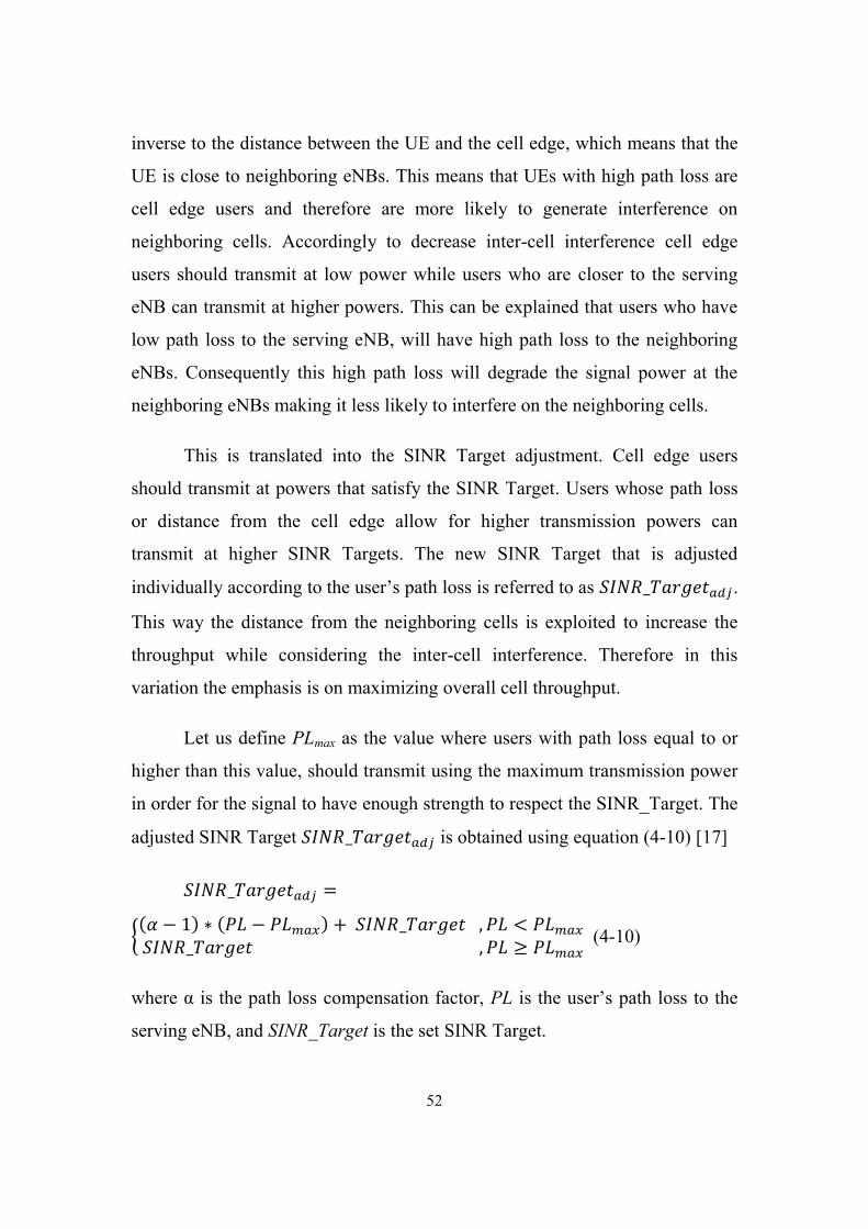
52
inverse to the distance between the UE and the cell edge, which means that the
UE is close to neighboring eNBs. This means that UEs with high path loss are
cell edge users and therefore are more likely to generate interference on
neighboring cells. Accordingly to decrease inter-cell interference cell edge
users should transmit at low power while users who are closer to the serving
eNB can transmit at higher powers. This can be explained that users who have
low path loss to the serving eNB, will have high path loss to the neighboring
eNBs. Consequently this high path loss will degrade the signal power at the
neighboring eNBs making it less likely to interfere on the neighboring cells.
This is translated into the SINR Target adjustment. Cell edge users
should transmit at powers that satisfy the SINR Target. Users whose path loss
or distance from the cell edge allow for higher transmission powers can
transmit at higher SINR Targets. The new SINR Target that is adjusted
individually according to the user’s path loss is referred to as .
This way the distance from the neighboring cells is exploited to increase the
throughput while considering the inter-cell interference. Therefore in this
variation the emphasis is on maximizing overall cell throughput.
Let us define PLmax as the value where users with path loss equal to or
higher than this value, should transmit using the maximum transmission power
in order for the signal to have enough strength to respect the SINR_Target. The
adjusted SINR Target is obtained using equation (4-10) [17]
{
(4-10)
where α is the path loss compensation factor, PL is the user’s path loss to the
serving eNB, and SINR_Target is the set SINR Target.

53
The above equation shows that users with path loss that give the user
power headroom to use higher transmission power will have a higher SINR
Target. Power headroom is the difference between the transmission power and
the maximum allowed transmission power. Therefore equation (4-10) increases
the SINR_Target for users closer to the eNB (have lower path loss).
The LTE PUSCH power control adjustment state is given by the
function . The function can represent either accumulation or current
absolute value. In this study it is considered to represent current absolute value.
In the case of current absolute value, the values taken by in dB are {-4,-
1,1,4}.
The adjusted SINR Target and the received SINR are entered into a
mapping function to obtain the value of . The mapping function is
described in Figure 4-5.
1. Calculate difference between received SINR and adjusted SINR Target
2. Using the SINR difference calculate the required transmission power needed to
be added to the received SINR to reach the adjusted SINR Target.
3. Obtain the TPC command as follows
If Prequired ≤ -4 then TPC = -4
elseif -4 < Prequired ≤ -1 then TPC = -1
elseif -1 < Prequired ≤ 1 then TPC = 1
else TPC = 4
endif
Figure 4-5 : Mapping Function

54
4.6.2 TPC Scheme 2: Total Generated Interference Limit
In the second scheme instead of setting an individual SINR Target, a
total target on the overall cell interference is set. In other words, a maximum
limit for the total interference generated by all the users in one cell is set. For
simplicity the cell interference limit is divided among the users in the cell such
that each user will have an interference limit it has to respect.
4.6.2.1 Interference Limit Distribution Among the Users
To divide the interference limit on the users present in the cell, there are
three different options.
Option1: The interference limit is equally divided among the users. This
provides the simplest solution and at the same time provides fairness among the
users as well as expected improved interference performance metrics. The
downside of using this option is that the large distance of the cell center users
from the cell edge is not exploited to increase throughput, neither are the cell
edge users given any advantage on the cell center users to compensate for their
large path loss. Therefore while this option provides a simple solution with
good performance in terms of throughput, it does not provide improved
Mapping Function - Adjusted SINR Target
Rec
eived
SIN
R
Figure 4-6 : Calculating TPC command Scheme 1
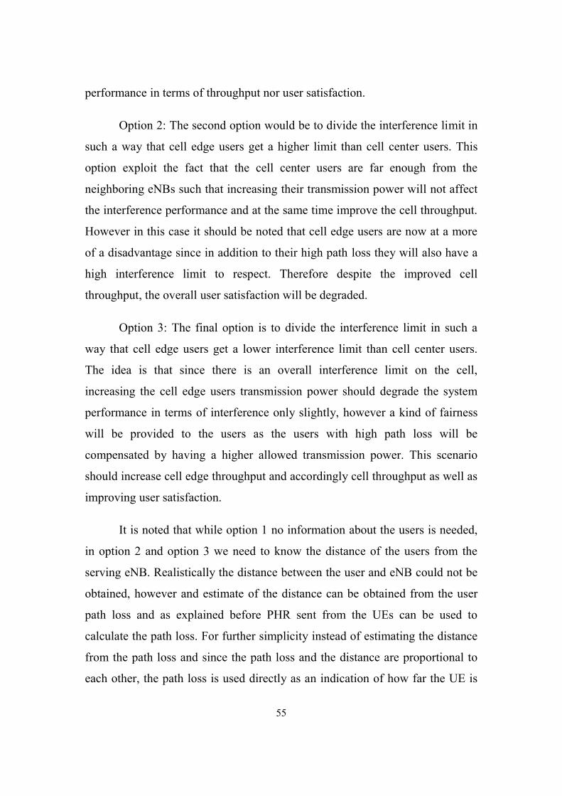
55
performance in terms of throughput nor user satisfaction.
Option 2: The second option would be to divide the interference limit in
such a way that cell edge users get a higher limit than cell center users. This
option exploit the fact that the cell center users are far enough from the
neighboring eNBs such that increasing their transmission power will not affect
the interference performance and at the same time improve the cell throughput.
However in this case it should be noted that cell edge users are now at a more
of a disadvantage since in addition to their high path loss they will also have a
high interference limit to respect. Therefore despite the improved cell
throughput, the overall user satisfaction will be degraded.
Option 3: The final option is to divide the interference limit in such a
way that cell edge users get a lower interference limit than cell center users.
The idea is that since there is an overall interference limit on the cell,
increasing the cell edge users transmission power should degrade the system
performance in terms of interference only slightly, however a kind of fairness
will be provided to the users as the users with high path loss will be
compensated by having a higher allowed transmission power. This scenario
should increase cell edge throughput and accordingly cell throughput as well as
improving user satisfaction.
It is noted that while option 1 no information about the users is needed,
in option 2 and option 3 we need to know the distance of the users from the
serving eNB. Realistically the distance between the user and eNB could not be
obtained, however and estimate of the distance can be obtained from the user
path loss and as explained before PHR sent from the UEs can be used to
calculate the path loss. For further simplicity instead of estimating the distance
from the path loss and since the path loss and the distance are proportional to
each other, the path loss is used directly as an indication of how far the UE is

56
from the serving eNB.
The interference limit ILi for each user i can be calculated by the
following equation:
∑ (4-11)
∑ (4-12)
where CIL is the cell interference limit in watts, and wi is the weight of user i.
According to which option will be implemented the weights of the users are
determined. For option 1, wi = 1, i, for option 2,
{ }, and for option 3, { }
where wi =1 for the user with average path loss for both options 2 and 3. The
values for the weights are obtained by experimenting with different sets of
values until a set is reached which provides good performance.
Note: The sum of the weights is not necessarily equal to one, but the sum of the
interference limits per user is equal to the cell interference limit CIL as
indicated in equation (4-12).
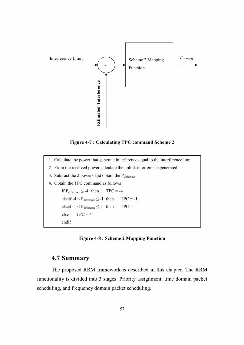
57
4.7 Summary
The proposed RRM framework is described in this chapter. The RRM
functionality is divided into 3 stages. Priority assignment, time domain packet
scheduling, and frequency domain packet scheduling.
Scheme 2 Mapping
Function -
Interference Limit
Est
ima
ted
In
terf
eren
ce
1. Calculate the power that generate interference equal to the interference limit
2. From the received power calculate the uplink interference generated.
3. Subtract the 2 powers and obtain the Pdifference
4. Obtain the TPC command as follows
If Pdifference ≤ -4 then TPC = -4
elseif -4 < Pdifference ≤ -1 then TPC = -1
elseif -1 < Pdifference ≤ 1 then TPC = 1
else TPC = 4
endif
Figure 4-7 : Calculating TPC command Scheme 2
Figure 4-8 : Scheme 2 Mapping Function

58
The priority assignment and the time domain packet scheduler are
mainly concerned with meeting the QoS requirements. The frequency domain
packet scheduler performs channel dependant scheduling with contiguity
constraint, AMC and power control.
ICIC was implemented through two power control algorithms. The first
algorithm controlled the users’ power individually, while the second algorithm
handled the power control on a cell level.

59
Chapter 5
System Model and Results Analysis
5.1 System Model
The simulated system is based on the 3GPP LTE. The scope of this
thesis is the uplink transmission only which use SC-FDMA as the radio access
technology.
Simulations are carried out using MATLAB code. The channels are
generated using the WINNER II Channel Models [25].
The system is simulated as a single cell of radius 500 m using the
suburban macro-cell scenario C1. In suburban macro-cells the eNB is located
well above the rooftops and UEs are outdoors at street level. Buildings are
typically low residential detached houses with one or two floors, or blocks of
flats with a few floors. Occasional open areas such as parks or playgrounds
between the houses make the environment rather open. Streets do not form
urban-like regular strict grid structure. Vegetation is modest.
The path loss models used in the WINNER II are of the form
(
) (5-1)
where d is the distance between the transmitter and receiver in [m], fc is the
center frequency in [GHz], the fitting parameter A includes the path loss
exponent, B is the intercept, C describes the path loss frequency dependence,
and X is an optional environment specific term.
For suburban macro-cell C1 scenarios, A=23.8, B=41.2 and C=20,

60
heNB=25 m, hUE=1.5 m
Table 5-1 : Path loss Model for C1 WINNER II Scenario [25]
LOS
⁄
σ=4 30 m<d<dBP
σ=6 dBP<d<5 Km
NLOS
⁄ σ=8 50 m<d<5 Km
The center frequency according to the LTE specification fc=2GHz.
According to [29], the LTE specifications support spectrum flexibility
by having a list of spectrum allocations. This allow mobile operators to choose
the spectrum allocation which is suitable for the user density in an area. The
lower the user density the smaller the bandwidth they need and therefore this
allows them to save on the bandwidth they purchase. Table 5-2 show the
allowed spectrum allocations and their corresponding transmission bandwidth
measured in terms of number of PRBs.
Table 5-2 : Transmission bandwidth configuration NRB in E-UTRA channel
bandwidths [29]
Channel bandwidth BWChannel [MHz]
1.4 3 5 10 15 20
Transmission bandwidth configuration NRB
6 15 25 50 75 100
The users belong to one of four traffic classes : VoIP, FTP, Interactive
Gaming and Video Streaming according to the distribution shown in Table 5-3.
The overall system parameters used in the simulations are shown in Table 5-4.

61
Table 5-3 : Traffic Classes Distribution
Traffic Class Percentage
VoIP 30%
FTP 30%
Interactive Gaming 20%
Video Streaming 20%
Table 5-4 : Simulation Parameters Summary
Parameter Setting
Number of simulation
runs 10
Simulation run duration 60 seconds
Center Frequency 2GHz
System Bandwidth 10MHz
Subcarrier Spacing 15KHz
FFT Size 1024
Fs 15.36MHz
Channel Model C1 – Suburban Macro-cell
User Speed 60m/s
Number of OFDM
symbols per slot 7
Slot Duration 0.5ms
TTI 1ms
Noise Power -160dBm/Hz
Rx Noise Figure 5dB
Maximum User Power 24dBm
α [18] 0.8
Po [18] -81dBm/Hz
Number of users 100
SINR Target 1dB
5.1.1 Calculating FFT Size and Sampling Frequency
To transform from time domain to frequency domain, FFT is employed
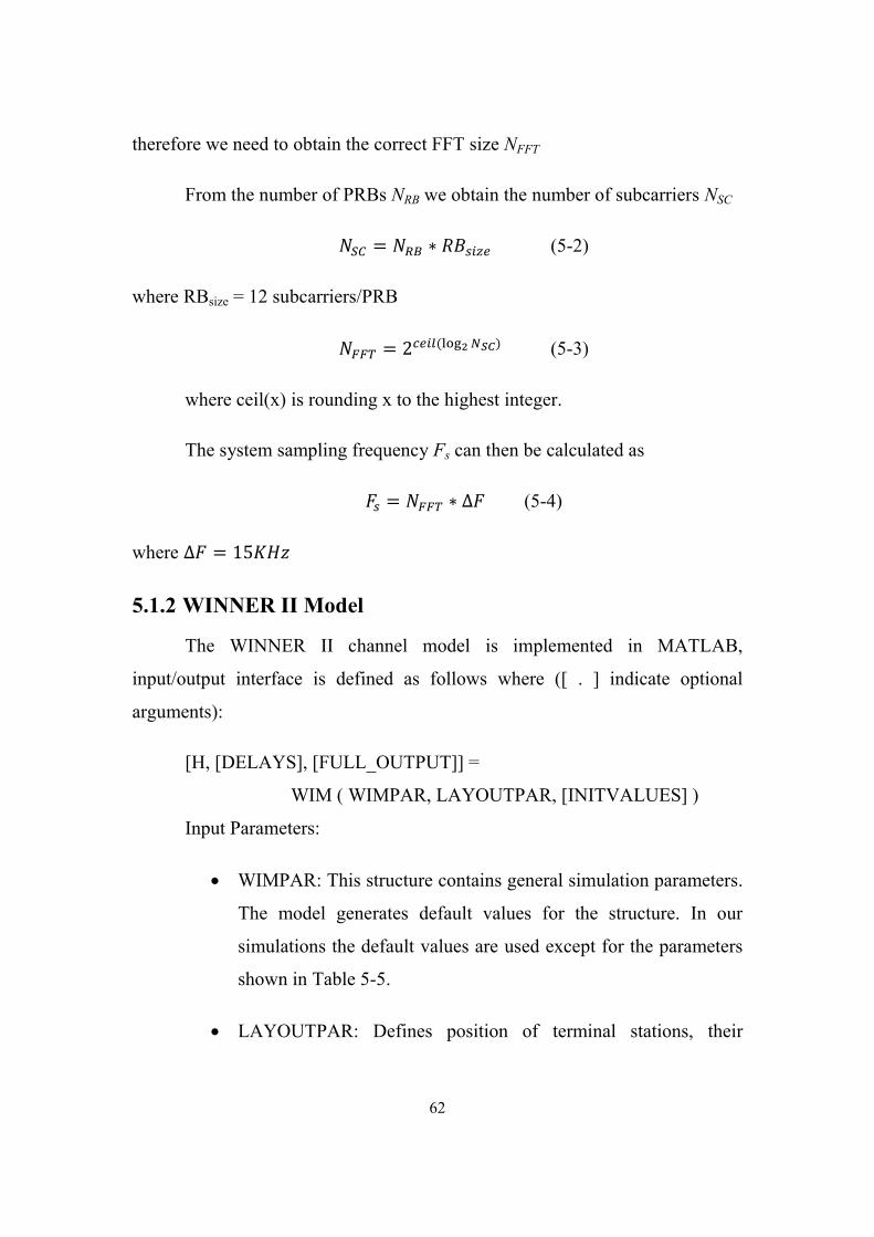
62
therefore we need to obtain the correct FFT size NFFT
From the number of PRBs NRB we obtain the number of subcarriers NSC
(5-2)
where RBsize = 12 subcarriers/PRB
(5-3)
where ceil(x) is rounding x to the highest integer.
The system sampling frequency Fs can then be calculated as
(5-4)
where
5.1.2 WINNER II Model
The WINNER II channel model is implemented in MATLAB,
input/output interface is defined as follows where ([ . ] indicate optional
arguments):
[H, [DELAYS], [FULL_OUTPUT]] =
WIM ( WIMPAR, LAYOUTPAR, [INITVALUES] )
Input Parameters:
WIMPAR: This structure contains general simulation parameters.
The model generates default values for the structure. In our
simulations the default values are used except for the parameters
shown in Table 5-5.
LAYOUTPAR: Defines position of terminal stations, their

63
assigned antenna arrays and gives links of interest for simulation.
INITVALUES: Parameters of the propagation channel. When
this parameter is given WIM does not generate the channel
parameters randomly, but uses the supplied initial channel values.
Output Parameters:
H: MIMO channel 5Dimensional-matrix which is collection of
time-variant Channel Impulse Responses (CIRs) (=f(t,τ)) between
all (Tx,Rx) pairs, for all links defined.
DELAYS: Multipath delays for all links, given in seconds.
FULL_OUTPUT: Stores the randomly generated link parameters
and the final phases of the complex sinusoids. This MATLAB
structure can be used as INITVALUES in subsequent function
calls to generate time continuous channel realizations with
separate function calls.
Table 5-5 : WIMPAR parameters values
Parameter Name Value
CenterFrequency 2GHz
NumTimeSamples 1000
SampleDensity 1.2491
PathLossModelUsed ‘No’
ShadowingModelUsed ‘No’
5.1.2.1 Calculating SampleDensity
The sample density represents the number of time samples per half
wavelength which indicates the sampling frequency of the channel. Therefore
to obtain the required sampling frequency we must set the SampleDensity
64
correctly.
(5-5)
where slight is the speed of light and equals 299792458m/s, fc is the carrier
frequency, vUE is the velocity of the UE and Tchannel is the channel sampling
time.
For fast fading channels the channel sampling time is the system
sampling time. This is the case when we are interested in the channel at every
time instant for example when we need to convolve the channel with a bit
stream. In this case we set ⁄ .
Flat fading is where we assume that the channel is constant with no
variations during a block of time. For flat fading channels the channel sampling
time is the block time. This is the case when we are interested in the channel
value at certain instances for example at the beginning of each TTI.
In our scheme, we schedule users on each TTI, so channel variations
lower than one TTI are not captured and therefore we set the channel sampling
time to flat fading with
5.1.2.2 Transforming Channel Matrix to Frequency Domain
The output of the WINNER model is a cell array of length equal to the
number of links. Each element in the array is a 4-D (UxSxTxN) channel matrix
h.
U: Number of receiver elements
S: Number of transmitter elements
T: Number of time samples
65
N: Number of paths/taps
The output matrix is in the time domain and since all our work is on
PRBs in the frequency domain we need to transform the channel matrix from
the time domain to the frequency domain using FFT. Before applying FFT the
channel matrix needs to be adjusted following the below steps:
1- The channel matrix resulting from the WINNER model may contain
Not any Number (NaN) values, which are MATLAB representation
for invalid values. Remove NaN values from the channel matrix
2- Round the delays of the different paths to the nearest multiple of the
system sampling time Ts=1/Fs.
3- Sum the taps that have the same delay
4- For the delays that have no taps insert zeros. e.g if we take Ts = 5
msec, we should have taps(path values) at delays 0,5,10,15 etc, there
could exist taps/paths at 0,10,15 so we need to insert 0 at the second
position in the taps array.
5- Normalize the channel energy
6- Perform FFT on the adjusted channel
5.1.3 Traffic Models
5.1.3.1 FTP Traffic Model
FTP traffic model is based on a Bernoulli process. Packets are generated
every 5 msec with probability 0.5. The packet size follows a uniform
distribution with the parameters shown in Table 5-6.
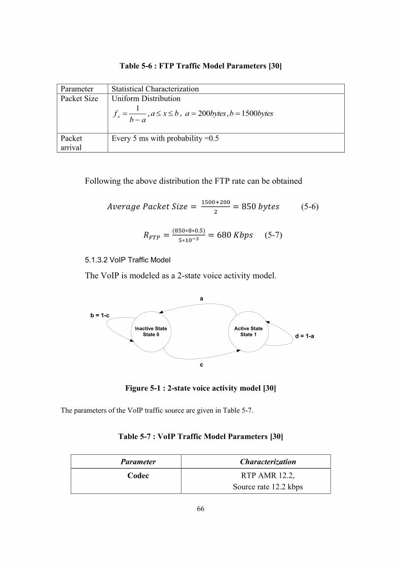
66
Table 5-6 : FTP Traffic Model Parameters [30]
Parameter Statistical Characterization
Packet Size Uniform Distribution
bxaab
f x
,1
, bytesbbytesa 1500,200
Packet
arrival
Every 5 ms with probability =0.5
Following the above distribution the FTP rate can be obtained
(5-6)
(5-7)
5.1.3.2 VoIP Traffic Model
The VoIP is modeled as a 2-state voice activity model.
Inactive State
State 0
Active State
State 1
a
c
d = 1-a
b = 1-c
Figure 5-1 : 2-state voice activity model [30]
The parameters of the VoIP traffic source are given in Table 5-7.
Table 5-7 : VoIP Traffic Model Parameters [30]
Parameter Characterization
Codec RTP AMR 12.2,
Source rate 12.2 kbps
67
Encoder frame length 20 ms
Voice activity factor
(VAF)
50% (c=0.01, d=0.99)
SID payload Modeled
15 bytes (5 Bytes + header)
SID packet every 160 ms during
silence
Protocol Overhead
with compressed header
10 bit + padding (RTP-pre-header)
4 Byte (RTP/UDP/IP)
2 Byte (RLC/security)
16 bits (CRC)
Total voice payload on
air interface
40 bytes (AMR 12.2)
Following the above distribution the VoIP rate can be obtained
(5-8)
Note: The 12.2 Kbps is the source rate that is it is the rate of the voice
data without any overheads in the active state.
5.1.3.3 Gaming Traffic Model
The gaming traffic model follow the distribution and parameters shown
in Table 5-8.
Table 5-8 : Uplink Gaming Network Traffic Parameters [30]
Parameter Statistical Characterization
Initial packet
arrival
Uniform Distribution
bxaab
f x
,1
, msba 40,0
Packet
arrival
Deterministic, 40 ms

68
Packet size Largest Extreme Value Distribution (also known as Fisher-Tippett
distribution)
b
ax
eb
ax
x eeb
f
1
, 7.5,45 bBytesa
Values for this distribution can be generated by the following
procedure:
ybax lnln , where y is drawn from a uniform distribution in
the range 1,0
Because packet size has to be integer number of bytes, the largest
integer less than or equal to x is used as the actual packet size
UDP header Deterministic (2 Bytes). This is added to the packet size accounting
for the UDP header after header compression.
Following the above distribution the gaming rate can be obtained
(5-9)
5.1.3.4 Video Streaming Traffic Model
Video data is divided into frames where each of these frames is
decomposed into a fixed number of slices each transmitted as a single packet.
The size of these packets and their inter-arrival time are modeled to have a
truncated Pareto distribution, while the number of packets in a frame and the
inter-arrival time between frames is deterministic. The traffic model assumes a
source video rate of 64 Kbps with other parameters and distributions defined in
Table 5-9.
Table 5-9 : Video Streaming Traffic Parameters [30]
Parameter Statistical Characterization
Inter-Arrival time
between the
beginning of each
frame
Deterministic
100 ms (based on 10 frames per second)
Number of packets
(slices) in a frame
Deterministic, 8 packets per frame

69
Packet (slice) size Truncated Pareto Distribution
Minimum= 53 Bytes, Mean=100 Bytes, Maximum =250 Bytes
(Before Truncation)
PDF: mxkf k
x
,1
, mxm
kf x
,
,
,20,2.1 Bytesk
Inter-arrival time
between packets
(slices) in a frame
Truncated Pareto Distribution
Minimum= 2.5 ms, Mean=m=6 ms, Maximum =12.5 ms (Before
Truncation)
PDF: mxkf k
x
,1
, mxm
kf x
,
, msk 5.2,2.1
Following the above distribution the video rate can be obtained
(5-10)

70
5.2 Simulation Results
5.2.1 Fixed Load and Fixed SINR Target
5.2.1.1 Comparison Algorithm
The proposed RRM framework is compared to the First Maximum
Expansion (FME) algorithm described in [3]. Results for the throughput and
packet delay are obtained for both the RRM framework and the FME
algorithm. The main idea of the FME algorithm is starting the assignment with
the PRB that has the highest metric value and “expanding” the assignment on
both sides of the allocation matrix. The metric could be the proportional fair
metric, or the channel gain. The algorithm steps are summarized below:
1- Search for highest metric in matrix and assign the RB to this UE (UE0-
RB0)
2- Check for the maximum value of the metric in the column on the left and
right of the assigned RB0. Expand in the direction of the higher maximum.
3- In the chosen direction for column by column get the maximum metric in
this column. Assign this RB to the UE with this highest metric if the
contiguity condition is not broken, otherwise to the UE assigned in the
previous column. Repeat until all the columns in this direction are assigned.
4- Repeat step 3 for the other direction.

71
5.2.1.2 Calculation of maximum achievable throughput and moving average
parameters
To have a benchmark to compare the simulation results with we
calculate the maximum achievable throughput for the current TTI. The
maximum achievable throughput is calculated by obtaining the set of active
users and allocating a PRB to the user who has highest channel gain on this
PRB. For the calculation of the maximum achievable throughput the contiguity
constraint is neglected.
A moving average is calculated for the maximum achievable throughput
and the throughput per TTI
The moving average of parameter X is calculated as
(5-11)
where we set α=0.8, giving higher weight to the average than the instantaneous
value.
5.2.1.3 Fixed Load and Fixed SINR Target Results
The simulation is carried out according to the default parameters in
Table 5-4 and the traffic mix in Table 5-3.
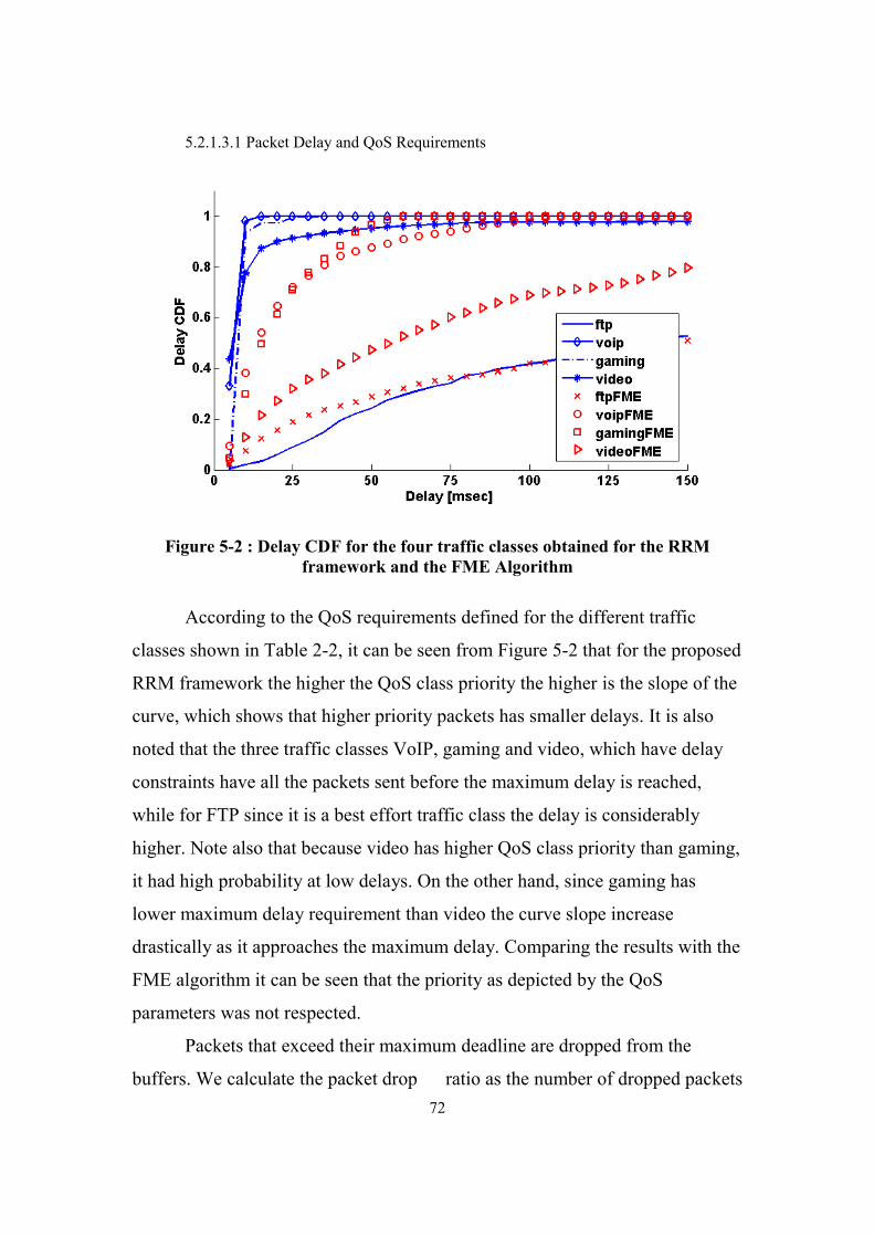
72
5.2.1.3.1 Packet Delay and QoS Requirements
Figure 5-2 : Delay CDF for the four traffic classes obtained for the RRM
framework and the FME Algorithm
According to the QoS requirements defined for the different traffic
classes shown in Table 2-2, it can be seen from Figure 5-2 that for the proposed
RRM framework the higher the QoS class priority the higher is the slope of the
curve, which shows that higher priority packets has smaller delays. It is also
noted that the three traffic classes VoIP, gaming and video, which have delay
constraints have all the packets sent before the maximum delay is reached,
while for FTP since it is a best effort traffic class the delay is considerably
higher. Note also that because video has higher QoS class priority than gaming,
it had high probability at low delays. On the other hand, since gaming has
lower maximum delay requirement than video the curve slope increase
drastically as it approaches the maximum delay. Comparing the results with the
FME algorithm it can be seen that the priority as depicted by the QoS
parameters was not respected.
Packets that exceed their maximum deadline are dropped from the
buffers. We calculate the packet drop ratio as the number of dropped packets

73
relative to the total number of generated packets. Results for the FME overall
packet drop ratio is around 40%. For the proposed RRM framework no packets
were dropped for VoIP and video traffic, while gaming and FTP had packet
drop ratios in the ranges of 10-3
and 10-2
, showing that the PELR QoS
parameter as depicted in Table 2-2 has been respected as well.

74
5.2.1.3.2 Cell Throughput
Figure 5-3 : Cell Throughput simulated for the RRM Framework and the FME
algorithm and compared to the maximum achievable throughput.
Figure 5-3 shows the maximum attainable throughput for the system and
also the achieved throughput using our RRM framework and the FME
algorithm. The plots are for the moving average of the maximum attainable
throughput and the achieved throughput. Although the FME algorithm give
higher throughput due to its usage of maximum transmission power and
allocations of PRBs based only on channel conditions, it is seen that the
proposed RRM framework yields throughput that is very close to the FME, it is
noted that for the RRM framework due to respecting the QoS parameters and
respecting the packets’ deadlines this helped in avoiding high packet drop rates.
It should be noted that the achieved throughput will always be less than
the maximum achievable throughput due to:

75
1. Contiguity constraint: PRBs assigned to one user must be
contiguous, which means that a PRB can be assigned to a user
who is not the best candidate for this PRB, from the point of view
of channel conditions, or a PRB can be assigned to a user who
does not need the PRB to send data on but the PRB is assigned as
it is in between PRBs assigned to this user.
2. QoS constraints: The QoS constraints are reflected in the user’s
priority, a PRB can be assigned to a user who is not the best
candidate since this user has higher priority than other users and
is served first.
3. Request constraint: The PRBs are assigned depending on the
user’s request. A user can be the best candidate for a PRB and is
not assigned this PRB since he does not need it and his request is
already fulfilled.
4. The inter-cell interference strategy that limits the transmission
power.

76
5.2.1.3.3 Generated Interference
Figure 5-4 : Total generated uplink interference for the proposed RRM
framework and the FME algorithm
Figure 5-4 shows the total generated uplink interference on neighboring
cells. It can be seen that with no power control mechanism as is the case with
the FME algorithm, high values of the generated interference are obtained,
while a considerable performance gain is obtained by using power control.
Since this evaluation is done considering a single cell, we can conjecture that in
a multi-cell environment, the performance of schemes without power control
will have an impact on throughput due to the increased interference from
neighboring cells. From Figures 5-3 and 5-4 it can be seen that the effect of the
tradeoff between minimizing inter-cell interference and maximizing throughput
can be handled through having an integrated framework which considers both
factors in the assignment.
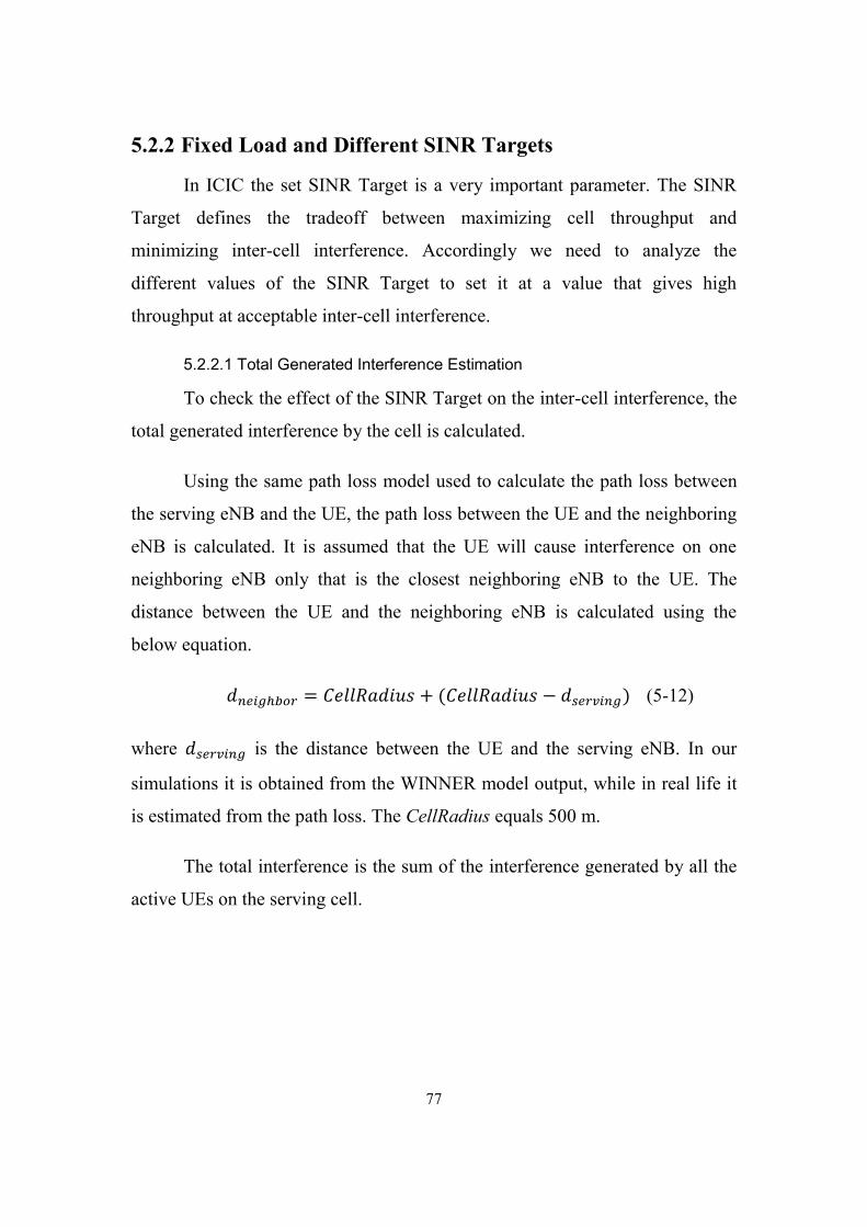
77
5.2.2 Fixed Load and Different SINR Targets
In ICIC the set SINR Target is a very important parameter. The SINR
Target defines the tradeoff between maximizing cell throughput and
minimizing inter-cell interference. Accordingly we need to analyze the
different values of the SINR Target to set it at a value that gives high
throughput at acceptable inter-cell interference.
5.2.2.1 Total Generated Interference Estimation
To check the effect of the SINR Target on the inter-cell interference, the
total generated interference by the cell is calculated.
Using the same path loss model used to calculate the path loss between
the serving eNB and the UE, the path loss between the UE and the neighboring
eNB is calculated. It is assumed that the UE will cause interference on one
neighboring eNB only that is the closest neighboring eNB to the UE. The
distance between the UE and the neighboring eNB is calculated using the
below equation.
(5-12)
where is the distance between the UE and the serving eNB. In our
simulations it is obtained from the WINNER model output, while in real life it
is estimated from the path loss. The CellRadius equals 500 m.
The total interference is the sum of the interference generated by all the
active UEs on the serving cell.

78
5.2.2.2 Fixed Load and Different SINR Targets Results
The default simulation parameters defined in Table 5-4 are used with the
following exceptions.
Parameter Setting
Simulation run duration 30 seconds
Number of users 20
Users traffic type FTP
SINR Target range [-5 5] dB
Serving
eNB
Figure 5-5 : Cells Layout showing the serving cell and the neighboring cells
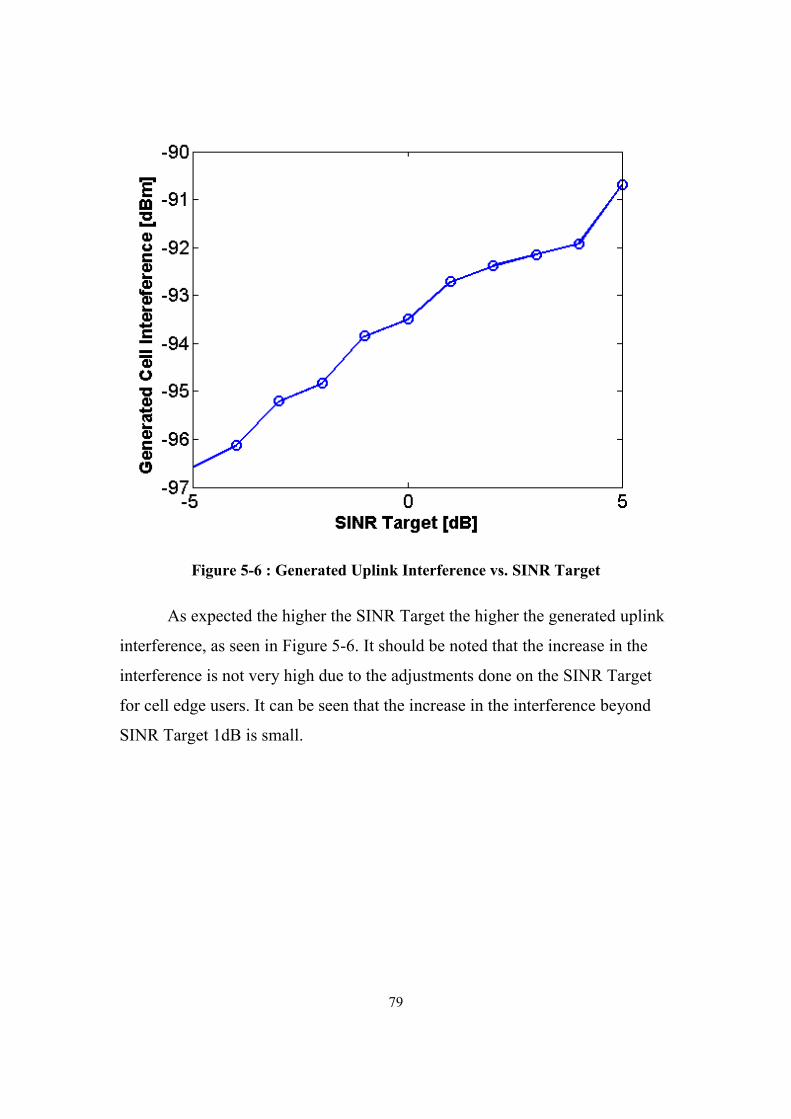
79
Figure 5-6 : Generated Uplink Interference vs. SINR Target
As expected the higher the SINR Target the higher the generated uplink
interference, as seen in Figure 5-6. It should be noted that the increase in the
interference is not very high due to the adjustments done on the SINR Target
for cell edge users. It can be seen that the increase in the interference beyond
SINR Target 1dB is small.

80
Figure 5-7 : Average Throughput vs. SINR Target
Higher SINR Targets means higher transmission power which is
mapped to higher MCS and therefore higher throughput. This is evident in
Figure 5-7. The high throughput values are due to the adjustments done on the
SINR Target for users far from the cell edge. Users who are near the cell center
and far from the cell edge are given an adjusted SINR Target which is higher
than the SINR Target, this allow them to transmit with higher power without
having concerns on the generated interference.
From the above graphs the optimum SINR Target can be chosen by
looking for the SINR Target that yields high throughput with an acceptable
generated interference.
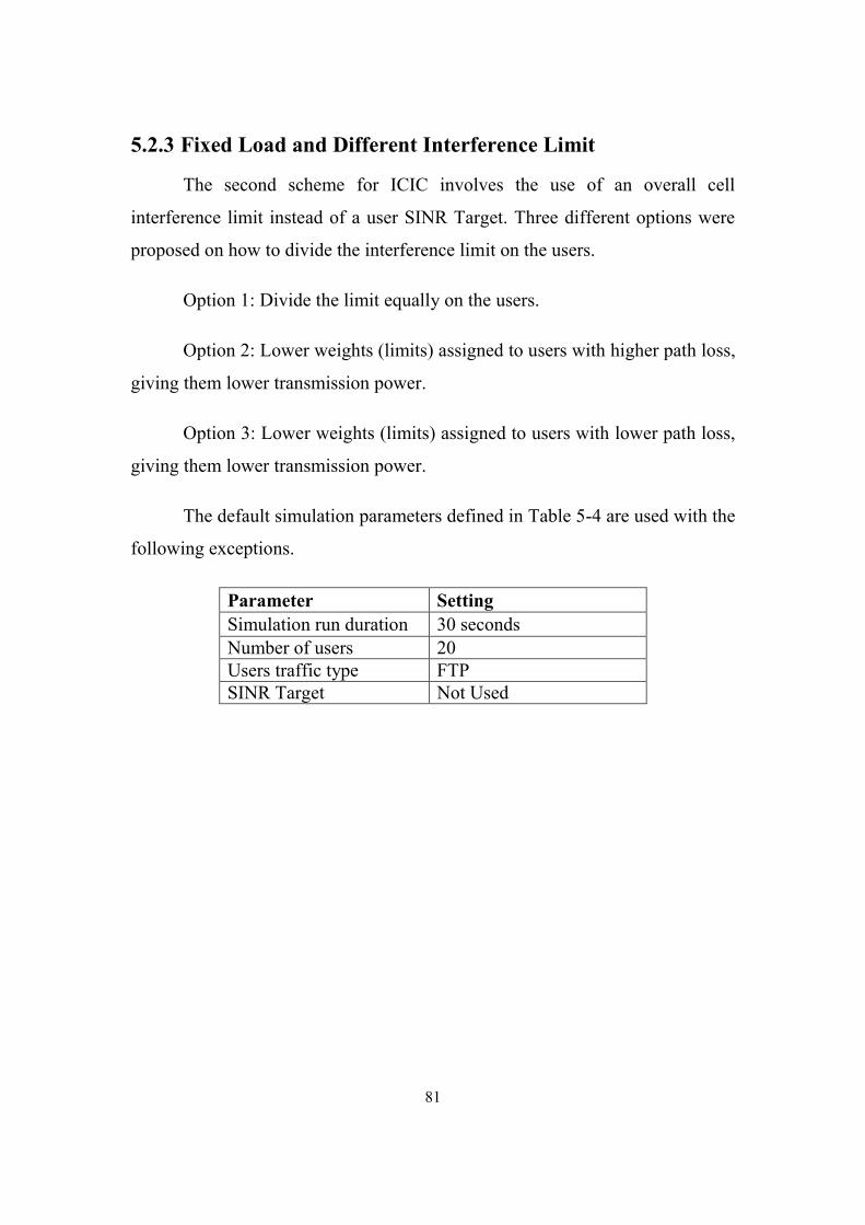
81
5.2.3 Fixed Load and Different Interference Limit
The second scheme for ICIC involves the use of an overall cell
interference limit instead of a user SINR Target. Three different options were
proposed on how to divide the interference limit on the users.
Option 1: Divide the limit equally on the users.
Option 2: Lower weights (limits) assigned to users with higher path loss,
giving them lower transmission power.
Option 3: Lower weights (limits) assigned to users with lower path loss,
giving them lower transmission power.
The default simulation parameters defined in Table 5-4 are used with the
following exceptions.
Parameter Setting
Simulation run duration 30 seconds
Number of users 20
Users traffic type FTP
SINR Target Not Used
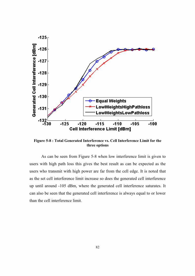
82
Figure 5-8 : Total Generated Interference vs. Cell Interference Limit for the
three options
As can be seen from Figure 5-8 when low interference limit is given to
users with high path loss this gives the best result as can be expected as the
users who transmit with high power are far from the cell edge. It is noted that
as the set cell interference limit increase so does the generated cell interference
up until around -105 dBm, where the generated cell interference saturates. It
can also be seen that the generated cell interference is always equal to or lower
than the cell interference limit.

83
Figure 5-9 : Overall Cell Throughput vs. Cell Interference Limit
Figure 5-9 shows the total cell throughput versus the cell interference
limit. As the interference limit decrease the throughput increase due to the
higher transmission power that can be used, until the power reach the
maximum allowed transmission power beyond which any decrease in the
interference limit do not have an effect on the throughput, this can be seen at
around -105 dBm. When low weights are given to users with high path loss this
means that users with low path loss will get higher weights leading to higher
limits and therefore they can transmit with higher powers, this leads to an
increase in the overall cell throughput as the users with good channel
conditions are favored.
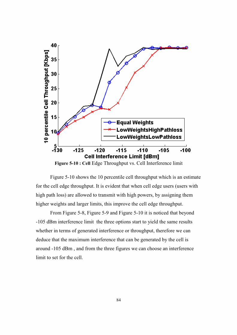
84
Figure 5-10 : Cell Edge Throughput vs. Cell Interference limit
Figure 5-10 shows the 10 percentile cell throughput which is an estimate
for the cell edge throughput. It is evident that when cell edge users (users with
high path loss) are allowed to transmit with high powers, by assigning them
higher weights and larger limits, this improve the cell edge throughput.
From Figure 5-8, Figure 5-9 and Figure 5-10 it is noticed that beyond
-105 dBm interference limit the three options start to yield the same results
whether in terms of generated interference or throughput, therefore we can
deduce that the maximum interference that can be generated by the cell is
around -105 dBm , and from the three figures we can choose an interference
limit to set for the cell.
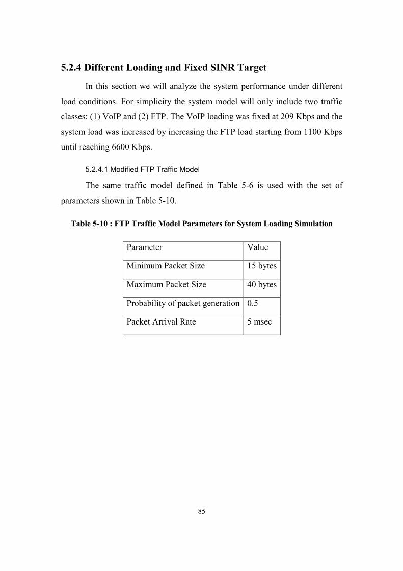
85
5.2.4 Different Loading and Fixed SINR Target
In this section we will analyze the system performance under different
load conditions. For simplicity the system model will only include two traffic
classes: (1) VoIP and (2) FTP. The VoIP loading was fixed at 209 Kbps and the
system load was increased by increasing the FTP load starting from 1100 Kbps
until reaching 6600 Kbps.
5.2.4.1 Modified FTP Traffic Model
The same traffic model defined in Table 5-6 is used with the set of
parameters shown in Table 5-10.
Table 5-10 : FTP Traffic Model Parameters for System Loading Simulation
Parameter Value
Minimum Packet Size 15 bytes
Maximum Packet Size 40 bytes
Probability of packet generation 0.5
Packet Arrival Rate 5 msec

86
5.2.4.2 Different Loading and Fixed SINR Target Results
Figure 5-11 : 95 percentile of delay Vs. Load
As can be seen from Figure 5-11, as long as the load is small and the
system bandwidth is sufficient the delay is almost near zero. As the number of
FTP load and accordingly the system load increase the delay increase. It is
noted that the VoIP delay start to increase slightly but remain within its limit of
50 msec when the FTP load reach 4400 Kbps, in comparison the FTP delay
increase dramatically when the system load increase. This shows that the QoS
parameters were respected and at the same time the delay of the best effort
traffic was minimized as much as the system can support, from this figure we
can estimate the system capacity beyond which the performance starts to
degrade.

87
Figure 5-12 : Throughput vs. FTP load
As can be expected as the load (number of users) increase the
throughput increase as seen in Figure 5-12, this is due to more efficient use of
the bandwidth as well as better exploitation of the multi user diversity.
However this is only applicable until we reach system saturation. As the
number of VoIP users is constant at 25 therefore the VoIP throughput is almost
constant, while as the number of FTP users increase the FTP throughput
increase as well.
88
Chapter 6
Conclusions and Future Work
6.1 Conclusions
In this thesis we proposed a complete radio resource management
framework for the LTE uplink transmission. The system model represented
multiple users with different channel conditions, QoS profiles and different
traffic generation parameters. The formulated problem is to determine on a TTI
basis the users who will be served in this TTI, the number and location of the
PRBs for each user, and the allocated MCS and power to transmit on these
PRBs.
It is shown from the literature that solving the frequency domain packet
scheduling problem alone is NP-hard therefore the problem of complete
resource management which is a more complex problem will be impractical to
solve optimally in real time systems. We proposed a heuristic three step
algorithm that solves the problem of complete resource management. The
framework maximizes the system throughput while minimizing the inter-cell
interference and considering the QoS requirements of the users.
The three main goals of the framework were: (1) Respect QoS
parameters of the different users, (2) Maximize system throughput, and (3)
Minimize inter-cell interference. To analyze the framework in terms of these
goals three simulation setups were done.
Simulation setup 1: Four different traffic types with different QoS
parameters and requirements were used. Fixed number of users and fixed
SINR_Target was also used. The simulation results show that the QoS
requirements represented by the packet delay and the packet error loss ratio of
the different classes have been satisfied while minimizing the reduction in

89
throughput.
Simulation setup 2: Fixed number of users belonging to four different
QoS classes is simulated. The SINR_Target was gradually increased to analyze
the effect on the inter-cell interference. It has been shown that there is a
tradeoff between maximizing throughput and minimizing inter-cell
interference.
Simulation setup 3: With fixed SINR_Target, number of users belonging
to two different QoS classes was increased gradually. The effect of system
loading has been analyzed in terms of throughput and packet delay. The
maximum system load beyond which the system is overloaded and contention
starts to occur is discovered.
6.2 Future Work
Two Inter-Cell Interference Coordination schemes were proposed in the
thesis, however simulations were done using a single cell. Future work will
include multi cell simulations to better study the schemes and how to enhance
them. In multi cell simulations there will be two types of networks:
homogenous and heterogeneous. Where the interference limit will be the same
for all cells in homogenous networks, the interference limit can be different for
different cells in heterogeneous networks. This will allow to study which type
of network has better performance as well as studying how the different
interference limits will be set for each cell in case of heterogeneous networks.
The proposed framework addressed some implementation issues of the
LTE standard. However some more aspects may be considered including,
Hybrid Automatic Repeat Request (HARQ), and actual available bandwidth for
allocation. The inclusion of the HARQ will have two effects. First a more
realistic implementation where perfect channel knowledge is not assumed will
90
be implemented, i.e. probability of erroneous transmissions and retransmissions
will be considered. The second effect is that the packet scheduler must consider
the HARQ retransmissions first, as according to the LTE standard HARQ
retransmissions must use the same PRBs used in the first transmission. as well
as that they have to be scheduled first before new transmissions.

91
REFERENCES
[1] S. Lee, I. Pefkianakis, A. Meyerson, S. Xu, and S. Lu,
"Proportional Fair Frequency-Domain Packet Scheduling for 3GPP
LTE Uplink", in Proc. INFOCOM, 2009, pp.2611-2615.
[2] F.D. Calabrese, P. Michaelsen, C. Rosa, M. Anas, C.U.
Castellanos, D.L. Villa, K.I. Pedersen, and P.E. Mogensen,
"Search-Tree Based Uplink Channel Aware Packet Scheduling for
UTRAN LTE", in Proc. VTC Spring, 2008, pp.1949-1953.
[3] L.Á.M.R.D. Temiño, G. Berardinelli, S. Frattasi, and P.E.
Mogensen, "Channel-aware scheduling algorithms for SC-FDMA
in LTE uplink", in Proc. PIMRC, 2008, pp.1-6.
[4] F. Liu, X. She, L. Chen, and H. Otsuka, "Improved Recursive
Maximum Expansion Scheduling Algorithms for Uplink Single
Carrier FDMA System", in Proc. VTC Spring, 2010, pp.1-5.
[5] F.D. Calabrese, C. Rosa, K.I. Pedersen, and P.E. Mogensen,
"Performance of Proportional Fair Frequency and Time Domain
Scheduling in LTE Uplink", in Proc. European Wireless, 2009,
pp.271-275.
[6] M. Al-Rawi, R. Jantti, J. Torsner and M. Sagfors, "Opportunistic
Uplink Scheduling for 3G LTE Systems," in Proc. 4th IEEE
Innovations in Information Technology, 2007, pp.705-709.
[7] M. Al-Rawi, R. Jäntti, J. Torsner, and M. Sågfors, "On the
performance of Heuristic opportunistic scheduling in the uplink of
3G LTE networks", in Proc. PIMRC, 2008, pp.1-6.
[8] H. Yang, F. Ren, C. Lin, and J. Zhang, "Frequency-Domain
Packet Scheduling for 3GPP LTE Uplink", in Proc. INFOCOM,
2010, pp.2597-2605.
[9] Y. Lin, and G. Yue, " Channel-Adapted and Buffer-Aware Packet
Scheduling in LTE Wireless Communication System", in Proc.
WiCOM, 2008, pp.1-4.
[10] G. Monghal, K.I. Pedersen, I.Z. Kovács, and P.E. Mogensen,
"QoS Oriented Time and Frequency Domain Packet Schedulers for
The UTRAN Long Term Evolution", in Proc. VTC Spring, 2008,

92
pp.2532-2536.
[11] K. Sandrasegaran, H.A.M. Ramli, and R. Basukala, "Delay-
Prioritized Scheduling (DPS) for Real Time Traffic in 3GPP LTE
System", in Proc. WCNC, 2010, pp.1-6.
[12] Y. Qian, C. Ren, S. Tang, and M. Chen, " Multi-service QoS
guaranteed based downlink cross-layer resource block allocation
algorithm in LTE systems", in Proc. WCNC, 2009, pp.1-4.
[13] O. Delgado and B. Jaumard, "Scheduling and Resource Allocation
in LTE Uplink with a Delay Requirement", in Proc. CNSR, 2010,
pp.268-275.
[14] Z. Li, C. Yin, and G. Yue, "Delay-Bounded Power-Efficient
Packet Scheduling for Uplink Systems of LTE", in Proc. WiCOM,
2009, pp.1-4.
[15] C.U. Castellanos, D.L. Villa, C. Rosa, K.I. Pedersen, F.D.
Calabrese, P. Michaelsen, and J. Michel, "Performance of Uplink
Fractional Power Control in UTRAN LTE", in Proc. VTC Spring,
2008, pp.2517-2521.
[16] A. Simonsson and A. Furuskar, "Uplink Power Control in LTE -
Overview and Performance, Subtitle: Principles and Benefits of
Utilizing rather than Compensating for SINR Variations", in Proc.
VTC Fall, 2008, pp.1-5.
[17] B. Muhammad, “Closed Loop Power Control for LTE Uplink”,
thesis presented as part of Degree of Master of Science in Electrical
Engineering , Blekinge Institute of Technology, November 2008.
[18] N. J. Quintero, “Advanced Power Control for UTRAN LTE
Uplink”, thesis submitted for the degree of Master of Science,
Department of Electronic Systems, Aalborg University, June 2008.
[19] M. Anas, “Uplink Radio Resource Management for QoS
Provisioning in Long Term Evolution With Emphasis on
Admission Control and Handover”, thesis presented as part of
degree of Doctor of Philosophy, Faculty of Engineering, Science
and Medicine of Aalborg University, January 2009.
[20] H.G. Myung, J. Lim, and D.J. Goodman, “Single carrier FDMA for
uplink wireless Transmission,” IEEE Veh. Technol. Mag., vol. 1,
93
no. 3, pp. 30–38, Sept. 2006.
[21] E. Dahlman, S. Parkvall, J. Skold, and P. Beming, 3G Evolution -
HSPA and LTE for Mobile Broadband, 1st ed. Academic Press,
2007.
[22] Next Generation Mobile Networks Forum, “Recommendation on
SON and O&M Requirements,” December 2008.
[23] 3rd Generation Partnership Project, “Self-Organizing Networks
(SON): Concepts and requirements,” TS 32.500 V9.0.0, Dec. 2009.
[24] C. Mehlführer, M. Wrulich, J. C. Ikuno, D. Bosanska and M. Rupp,
"Simulating the Long Term Evolution Physical Layer," in Proc. of
the 17th European Signal Processing Conference (EUSIPCO
2009), Aug. 2009, Glasgow, Scotland.
[25] WINNER II channel model
[26] Technical Specification Group Radio Access Network, “Evolved
universal terrestrial radio access (E-UTRA); physical layer
procedures,” 3rd Generation Partnership Project (3GPP), Tech.
Rep. TS 36.213, Mar. 2009.
[27] S. Sesia, I. Toufik, and M. Baker, LTE – The UMTS Long Term
Evolution From Theory to Practice, 1st ed. John Wiley & Sons,
2009.
[28] S. M. Shukry, K. Elsayed, A. Elmoghazy, and A. Nassar "Adaptive
fractional frequeny reuse (AFFR) scheme for multi-cell IEEE
802.16e systems," Proceeding of HONET'09, 2009.
[29] 3GPP TS 36.104 “3rd Generation Partnership Project; Technical
Specification Group Radio Access Network; Evolved Universal
Terrestrial Radio Access (E-UTRA); Base Station (BS) radio
transmission and reception (Release 10)”
[30] Orange, China Mobile, KPN, NTT DoCoMo, Sprint, T-Mobile,
Vodafone, Telecom Italia, “LTE physical layer framework for
performance verification,” R1-070674, 3GPP TSG-RAN1#48, St.
Louis, Mich, February, 2007.

ملخص
التحسن في الاداء في نظم "التطور البعيد المدى" اللاسلكية علي نظم "الجيل الثالث" تأتي علي
في هذه الرسالة نقدم اطار شامل لتوزيع الموارد فى حساب اضافة قيود و تحديات جديدة لتصميم النظام.
الاطار الشامل لتوزيع ة للارسال من المستخدم الى محطة البث. نظم "التطور البعيد المدى" اللاسلكي
وفقا لمواصفات نظم "التطور البعيد المدى" اللاسلكية للارسال من الموارد يحقق الوظائف الاتية
لارسال, التحكم في قوة الارسال, تخصيص عرض النطاق الترددي ل: المستخدم الى محطة البث
يز.تخصيص نظام التعديل و الترم
حامل –الأستخدام المتعدد للترددات المتعامدة "تحدد نظم "التطور البعيد المدى" تكنولوجيا
قبل أكثر من مستخدم فى نفس الوقت للارسال من أوحد" لاتاحة استخدام عرض النطاق الترددى من
قوة ارسال و يتم استخدام هذه التكنولوجيا لميزة صغر النسبة بين أعلى المستخدم الى محطة البث.
, و لكن هذه الميزة تفرض أن يكون تخصيص الحوامل التابعة لمستخدم ما متجاور متوسط قوة الارسال
مما يفرض قيد علي تصميم النظام.
مع التقدم في التكنولوجيا يوجد الان تطبيقات متعددة و يوجد لكل تطبيق تحديدات و متططلبات
لات عبر بروتوكول الانترنت تتطلب أن يكون التأخير في خاصة به. علي سبيل المثال تطبيق الاتصا
يتم أخذ هذه توصيل حزم المعلومات أقل ما يكون بينما تطبيقات بروتوكول نقل الملفات لا تتطلب ذلك.
التحكم في قوة عند .لارسالتخصيص عرض النطاق الترددي لالمتطلبات الختلفة في الاعتبار عند
بار قوة التداخل المولدة علي الخلايا الجاورة, فبالرغم من أن تخفيض قوة يجب الأخذ في الاعت الارسال
التداخل المولدة علي الخلايا الجاورة يؤدى الي تخفيض انتاجية الخلية الا أنها تؤدى الى زيادة انتاجية
لخدمة القدم النظام ككل. ألاطار المقترح يؤدى الى زيادة الانتاجية و الكفائة الطيفية بينما يراعى مستوى ا
لكل مستخدم بالاضافة الى تنفيذ نظام تنسيق التداخل بين الخلايا.

اطار شامل لتوزيع الموارد فى نظم "التطور البعيد المدى" اللاسلكية للارسال من
المستخدم الى محطة البث
إعداد
أميرة محمد يحيي عبدالهادى عفيفيم.
جامعة القاهرة –رسالة مقدمة إلى كلية الهندسة
كجزء من متطلبات الحصول على درجة الماجستير في
الاتصالات الكهربائيةوهندسة الإلكترونيات
يعتمد من لجنة الممتحنين
) عين شمس جامعة –أستاذ بكلية الهندسة ( عضو سلوى حسين الرملي .أ.د
( القاهرة جامعة –أستاذ بكلية الهندسة ( عضو محمد حازم محمد صبحى.أ.د
)جامعة القاهرة –أستاذ بكلية الهندسة ( مشرف الرسالة خالد محمد فؤاد السيد .أ.د
جامعة القاهرة –كلية الهندسة
جمهورية مصر العربية –الجيزة
م 2011 -هـ 1432

اطار شامل لتوزيع الموارد فى نظم "التطور البعيد المدى" اللاسلكية للارسال من
محطة البثالمستخدم الى
إعداد
أميرة محمد يحيي عبدالهادى عفيفيم.
جامعة القاهرة –رسالة مقدمة إلى كلية الهندسة
كجزء من متطلبات الحصول على درجة الماجستير في
الاتصالات الكهربائيةوهندسة الإلكترونيات
تحت إشراف
خالد محمد فؤاد السيد .د.أ
جامعة القاهرة –بكلية الهندسة أستاذ
جامعة القاهرة –كلية الهندسة
جمهورية مصر العربية –الجيزة
م 2011 -هـ 1432

اطار شامل لتوزيع الموارد فى نظم "التطور البعيد المدى" اللاسلكية للارسال من
المستخدم الى محطة البث
إعداد
م. أميرة محمد يحيي عبدالهادى عفيفي
جامعة القاهرة –رسالة مقدمة إلى كلية الهندسة
كجزء من متطلبات الحصول على درجة الماجستير في
هندسة الإلكترونيات والاتصالات الكهربائية
جامعة القاهرة –كلية الهندسة
جمهورية مصر العربية –الجيزة
م 2011 -هـ 1432