Linear regression and ANOVA - Amherst College · Linear regression and ANOVA Regression and analysis of variance form the basis of many investigations. In this chapter we describe

✐

✐

“book” — 2014/5/6 — 15:21 — page 113 — #137✐

✐

✐

✐

✐

✐

Chapter 6

Linear regression and ANOVA

Regression and analysis of variance form the basis of many investigations. In this chapterwe describe how to undertake many common tasks in linear regression (broadly defined),while Chapter 7 discusses many generalizations, including other types of outcome variables,longitudinal and clustered analysis, and survival methods.

Many SAS procedures and R commands can perform linear regression, as it constitutesa special case of which many models are generalizations. We present detailed descriptionsfor SAS proc reg and proc glm as well as for the R lm() command, as these offer themost flexibility and best output options tailored to linear regression in particular. WhileANOVA can be viewed as a special case of linear regression, separate routines are availablein SAS (proc anova) and R (aov()) to perform it. In addition, SAS proc mixed is neededfor some calculations. We address these additional procedures only with respect to outputthat is difficult to obtain through the standard linear regression tools.

R supports a flexible modeling language implemented using formulas (see help(formula)and 6.1.1) for regression that is shared with the lattice graphics functions. Many of the rou-tines available within R return or operate on lm class objects, which include objects suchas coefficients, residuals, fitted values, weights, contrasts, model matrices, and the like (seehelp(lm)).

The CRAN statistics for the social sciences task view provides an excellent overview ofmethods described here and in Chapter 7.

6.1 Model fitting

6.1.1 Linear regression

Example: 6.6.2SAS

proc glm data=ds;

model y = x1 ... xk;

run;orproc reg data=ds;


run;

Note: Both proc glm and proc reg support linear regression models, while proc reg pro-vides more regression diagnostics. The glm procedure more easily allows categorical covari-ates.

113

✐

✐

“book” — 2014/5/6 — 15:21 — page 114 — #138✐

✐

✐

✐

✐

✐

114 CHAPTER 6. LINEAR REGRESSION AND ANOVA

R

mod1 = lm(y ~ x1 + ... + xk, data=ds)

summary(mod1)

summary.aov(mod1)orform = as.formula(y ~ x1 + ... + xk)

mod1 = lm(form, data=ds)

summary(mod1)

coef(mod1)

Note: The first argument of the lm() function is a formula object, with the outcomespecified followed by the ∼ operator then the predictors. It returns a linear model ob-ject. More information about the linear model summary() command can be found us-ing help(summary.lm). The coef() function extracts coefficients from a model (see alsothe coefplot package). The biglm() function in the biglm package can support modelfitting to very large datasets. By default, stars are used to annotate the output of thesummary() functions regarding significance levels: these can be turned off using the com-mand options(show.signif.stars=FALSE). The biglm package can be used to undertakeestimation with larger datasets.

6.1.2 Linear regression with categorical covariates

Example: 6.6.2See 6.1.4 (parameterization of categorical covariates).

SAS

proc glm data=ds;

class x1;

model y = x1 x2 ... xk;

run;

Note: The class statement specifies covariates that should be treated as categorical. Theglm procedure uses reference cell coding; the reference category can be controlled using theorder option to the proc glm statement, as in 7.10.11.

R

ds = transform(ds, x1f = as.factor(x1))

mod1 = lm(y ~ x1f + x2 + ... + xk, data=ds)

Note: The as.factor() command in R creates a categorical variable from a variable. Bydefault, the lowest value (either numerically or lexicographically) is the reference value. Thelevels option for the factor() function can be used to select a particular reference value(see 2.2.19). Ordered factors can be constructed using the ordered() function.

6.1.3 Changing the reference category

SAS

proc sort data=ds;

by classvar;

run;

proc glm data=ds order=data;

class classvar;

model y = classvar;

run;

✐

✐

“book” — 2014/5/6 — 15:21 — page 115 — #139✐

✐

✐

✐

✐

✐

6.1. MODEL FITTING 115

orproc genmod data=ds;

class classvar (param=ref ref="level");

model y = classvar;

run;

Note: The first code is necessary for procedures that use the more primitive class state-ment, as reviewed in 6.1.4. For these procedures, the default reference category is the lastone. The order option can take other values, which may be useful. If the desired referencecell cannot be sorted to the end, it may be necessary to recode the category values to, e.g.,A. Brown, B. Blue, and C. Green from Blue, Brown, and Green, before sorting. Sorting bydescending classvar may also be useful. The second set of code will work in the genmod,logistic, and surveylogistic procedures.

R

ds = transform(ds, neworder = factor(classvar,

levels=c("level", "otherlev1", "otherlev2"))

mod1 = lm(y ~ neworder, data=ds)

Note: The first level of a factor (by default that which appears first lexicographically) isthe reference group. This can be modified through use of the factor() function.

6.1.4 Parameterization of categorical covariates

Example: 6.6.5SAS and R handle this issue in different ways. In R, as.factor() can be applied within anymodel-fitting function. Parameterization of the covariate can be controlled as below. ForSAS, some procedures accept a class statement to declare that a covariate is to be treatedas categorical. The following procedures will not accept a class statement: arima, catmod,factor, lifetest, loess, mcmc, nlin, nlmixed, reg, and varclus. For these procedures,indicator (or “dummy”) variables must be created in a data step, though this should bedone with caution. The following procedures accept a class statement which applies ref-erence cell or indicator variable coding (described as contr.SAS() in the R note below)to the listed variables: proc anova, candisc, discrim, fmm, gam, glimmix, glm, mixed,quantreg, robustreg, stepdisc, and surveyreg. The value used as the referent can oftenbe controlled, usually as an order option to the controlling proc, as in 7.10.11. For theseprocedures, other parameterizations must be coded in a data step. The following proceduresaccept multiple parameterizations, using the syntax shown below for proc logistic: procgenmod (defaults to reference cell coding), proc logistic (defaults to effect coding), procphreg (defaults to reference cell coding), and proc surveylogistic (defaults to effectcoding).

SAS

proc logistic data=ds;

class x1 (param=paramtype) x2 (param=paramtype);

...

run;orproc logistic data=ds;

class x1 x2 / param=paramtype;

...

run;

Note: Available paramtypes include: 1) orthpoly, equivalent to contr.poly(); 2) effect(the default for proc logistic and proc surveylogistic), equivalent to contr.sum();and 3) ref, equivalent to contr.SAS(). In addition, if the same parameterization is desired

✐

✐

“book” — 2014/5/6 — 15:21 — page 116 — #140✐

✐

✐

✐

✐

✐


for all of the categorical variables in the model, it can be added in a statement such asthe second example. In this case, param=glm can be used to emulate the parameterizationfound in the other procedures which accept class statements and in contr.SAS() withinR; this is the default for proc genmod and proc phreg.

R

ds = transform(ds, x1f = as.factor(x1))

mod1 = lm(y ~ x1f, contrasts=list(x1f="contr.SAS"), data=ds)

Note: The as.factor() function creates a factor object, akin to how SAS treatsclass variables in proc glm. The contrasts option for the lm() function specifies how thelevels of that factor object should be used within the function. The levels option to thefactor() function allows specification of the ordering of levels (the default is lexicographic).An example can be found in 6.6.

The specification of the design matrix for analysis of variance and regression modelscan be controlled using the contrasts option. Examples of options (for a factor with fourequally spaced levels) are given below.

> contr.treatment(4) > contr.poly(4)

2 3 4 .L .Q .C

1 0 0 0 [1,] -0.671 0.5 -0.224

2 1 0 0 [2,] -0.224 -0.5 0.671

3 0 1 0 [3,] 0.224 -0.5 -0.671

4 0 0 1 [4,] 0.671 0.5 0.224

> contr.SAS(4) > contr.sum(4)

1 2 3 [,1] [,2] [,3]

1 1 0 0 1 1 0 0

2 0 1 0 2 0 1 0

3 0 0 1 3 0 0 1

4 0 0 0 4 -1 -1 -1

> contr.helmert(4)

[,1] [,2] [,3]

1 -1 -1 -1

2 1 -1 -1

3 0 2 -1

4 0 0 3

See options("contrasts") for defaults, and contrasts() or lm() to apply a contrastfunction to a factor variable. Support for reordering factors is available within the factor()function.

6.1.5 Linear regression with no intercept

SAS

proc glm data=ds;

model y = x1 ... xk / noint;

run;

Note: The noint option works with many model statements.

R

mod1 = lm(y ~ 0 + x1 + ... + xk, data=ds)

ormod1 = lm(y ~ x1 + ... + xk - 1, data=ds)

✐

✐

“book” — 2014/5/6 — 15:21 — page 117 — #141✐

✐

✐

✐

✐

✐

6.1. MODEL FITTING 117

6.1.6 Linear regression with interactions

Example: 6.6.2SAS

proc glm data=ds;

model y = x1 x2 x1*x2 x3 ... xk;

run;orproc glm data=ds;

model y = x1|x2 x3 ... xk;

run;

Note: The | operator includes the product and all lower order terms, while the * operatorincludes only the specified interaction. So, for example, model y = x1|x2|x3 and model y

= x1 x2 x3 x1*x2 x1*x3 x2*x3 x1*x2*x3 are equivalent statements. The syntax abovealso works with any covariates designated as categorical using the class statement (6.1.2).The model statement for many procedures accepts this syntax.

R

mod1 = lm(y ~ x1 + x2 + x1:x2 + x3 + ... + xk, data=ds)

orlm(y ~ x1*x2 + x3 + ... + xk, data=ds)

Note: The * operator includes all lower order terms (in this case main effects), while the : op-erator includes only the specified interaction. So, for example, the commands y ∼ x1*x2*x3

and y ∼ x1 + x2 + x3 + x1:x2 + x1:x3 + x2:x3 + x1:x2:x3 are equivalent. The syn-tax also works with any covariates designated as categorical using the as.factor() com-mand (see 6.1.2).

6.1.7 One-way analysis of variance

Example: 6.6.5SAS

proc glm data=ds;

class x;

model y = x / solution;

run;

Note: The solution option to the model statement requests that the parameter estimatesbe displayed. Other procedures which fit ANOVA models include proc anova and proc

mixed.

R

ds = transform(ds, xf=as.factor(x))

mod1 = aov(y ~ xf, data=ds)

summary(mod1)

anova(mod1)

Note: The summary() command can be used to provide details of the model fit. Moreinformation can be found using help(summary.aov). Note that summary.lm(mod1) willdisplay the regression parameters underlying the ANOVA model.

6.1.8 Analysis of variance with two or more factors

Example: 6.6.5Interactions can be specified using the syntax introduced in 6.1.6 (see interaction plots,8.5.2).

✐

✐

“book” — 2014/5/6 — 15:21 — page 118 — #142✐

✐

✐

✐

✐

✐


SAS

proc glm data=ds;

class x1 x2;

model y = x1 x2;

run;

Note: Other procedures which fit ANOVA models include proc anova and proc mixed.

R

aov(y ~ as.factor(x1) + as.factor(x2), data=ds)

6.2 Tests, contrasts, and linear functions of parameters

6.2.1 Joint null hypotheses: several parameters equal 0

As an example, consider testing the null hypothesis H0 : β1 = β2 = 0.

SAS

proc reg data=ds;

model ...;

nametest: test x1=0, x2=0;

run;

Note: In the above, nametest is an arbitrary label which will appear in the output. Multipletest statements are permitted.

R



anova(mod2, mod1)

6.2.2 Joint null hypotheses: sum of parameters

As an example, consider testing the null hypothesis H0 : β1 + β2 = 1.

SAS

proc reg data=ds;

model ...;

nametest: test x1 + x2 = 1;

run;

Note: The test statement is prefixed with an arbitrary nametest which will appear in theoutput. Multiple test statements are permitted.

R


covb = vcov(mod1)

coeff.mod1 = coef(mod1)

t = (coeff.mod1[2] + coeff.mod1[3] - 1)/

sqrt(covb[2,2] + covb[3,3] + 2*covb[2,3])

pvalue = 2*(1-pt(abs(t), df=mod1$df))

Note: The I() function inhibits the interpretation of operators, to allow them to be usedas arithmetic operators.

✐

✐

“book” — 2014/5/6 — 15:21 — page 119 — #143✐

✐

✐

✐

✐

✐

6.2. TESTS, CONTRASTS, AND LINEAR FUNCTIONS OF PARAMETERS 119

6.2.3 Tests of equality of parameters

Example: 6.6.7As an example, consider testing the null hypothesis H0 : β1 = β2.

SAS

proc reg data=ds;

model ...;

nametest: test x1=x2;

run;

Note: The test statement is prefixed with an arbitrary nametest which will appear in theoutput. Multiple test statements are permitted.

R


mod2 = lm(y ~ I(x1+x2) + ... + xk, data=ds)

anova(mod2, mod1)orlibrary(gmodels)

estimable(mod1, c(0, 1, -1, 0, ..., 0))ormod1 = lm(y ~ x1 + ... + xk, data=ds)

covb = vcov(mod1)


t = (coeff.mod1[2]-coeff.mod1[3])/sqrt(covb[2,2]+covb[3,3]-2*covb[2,3])

pvalue = 2*(1-pt(abs(t), mod1$df))

Note: The I() function inhibits the interpretation of operators, to allow them to be usedas arithmetic operators. The estimable() function calculates a linear combination of theparameters. The more general R code below utilizes the same approach introduced in 6.2.1for the specific test of β1 = β2 (different coding would be needed for other comparisons).

6.2.4 Multiple comparisons

Example: 6.6.6SAS

proc glm data=ds;

class x1;

model y = x1;

lsmeans x1 / pdiff adjust=tukey;

run;

Note: The pdiff option requests p-values for the hypotheses involving the pairwise compar-ison of means. The adjust option adjusts these p-values for multiple comparisons. Otheroptions available through adjust include bon (for Bonferroni) and dunnett, among others.SAS proc mixed also has an adjust option for its lsmeans statement. A graphical presen-tation of significant differences among levels can be obtained with the lines option to thelsmeans statement, as shown in 6.6.6.

R

mod1 = aov(y ~ x, data=ds)

TukeyHSD(mod1, "x")

Note: The TukeyHSD() function takes an aov object as an argument and calculates thepairwise comparisons of all of the combinations of the factor levels of the variable x (seethe multcomp package).

✐

✐

“book” — 2014/5/6 — 15:21 — page 120 — #144✐

✐

✐

✐

✐

✐


6.2.5 Linear combinations of parameters

Example: 6.6.7It is often useful to calculate predicted values for particular covariate values. Here, wecalculate the predicted value E[Y |X1 = 1, X2 = 3] = β0 + β1 + 3β2.

SAS

proc glm data=ds;


estimate 'label' intercept 1 x1 1 x2 3;

run;

Note: The estimate statement is used to calculate a linear combination of parameters (andassociated standard errors). The optional quoted text is a label which will be printed withthe estimated function.

R

mod1 = lm(y ~ x1 + x2, data=ds)

newdf = data.frame(x1=c(1), x2=c(3))

predict(mod1, newdf, se.fit=TRUE, interval="confidence")orlibrary(gmodels)

estimable(mod1, c(0, 1, 3))orlibrary(mosaic)

myfun = makeFun(mod1)

myfun(x1=1, x2=3)

Note: The predict() command in R can generate estimates at any combination of param-eter values, as specified as a dataframe that is passed as an argument. More information onthis function can be found using help(predict.lm).

6.3 Model diagnostics

6.3.1 Predicted values

Example: 6.6.2SAS

proc reg data=ds;

model ...;

output out=newds predicted=predicted_varname;


model ...;

output out=newds predicted=predicted_varname;

run;

Note: The output statement creates a new dataset and specifies variables to be included,of which the predicted values are an example. Others can be found using the on-line help:Contents; SAS Products; SAS Procedures; REG; OUTPUT.

R

mod1 = lm(y ~ x, data=ds)

predicted.varname = predict(mod1)

Note: The command predict() operates on any lm object and by default generates a vectorof predicted values. Similar commands retrieve other regression output.

✐

✐

“book” — 2014/5/6 — 15:21 — page 121 — #145✐

✐

✐

✐

✐

✐

6.3. MODEL DIAGNOSTICS 121

6.3.2 Residuals

Example: 6.6.2SAS

proc glm data=ds;

model ...;

output out=newds residual=residual_varname;


model ...;

output out=newds residual=residual_varname;

run;

Note: The output statement creates a new dataset and specifies variables to be included, ofwhich the residuals are an example. Others can be found using the on-line help: Contents;SAS Products; SAS Procedures; REG; OUTPUT.

R


residual.varname = residuals(mod1)

Note: The command residuals() operates on any lm object and generates a vec-tor of residuals. Other functions for aov, glm, or lme objects exist (see, for example,help(residuals.glm)).

6.3.3 Standardized and Studentized residuals

Example: 6.6.2Standardized residuals are calculated by dividing the ordinary residual (observed minusexpected, yi − yi) by an estimate of its standard deviation. Studentized residuals are cal-culated in a similar manner, where the predicted value and the variance of the residual areestimated from the model fit while excluding that observation. In SAS proc glm the stan-dardized residual is requested by the student option, while the rstudent option generatesthe studentized residual.

SAS

proc glm data=ds;

model ...;

output out=newds student=standardized_resid_varname;


model ...;

output out=newds rstudent=studentized_resid_varname;

run;

Note: The output statement creates a new dataset and specifies variables to be included, ofwhich the Studentized residuals are an example. Both proc reg and proc glm include bothtypes of residuals. Others can be found using the on-line help: Contents; SAS Products; SASProcedures; REG; OUTPUT.

R


standardized.resid.varname = stdres(mod1)

studentized.resid.varname = studres(mod1)

Note: The stdres() and studres() functions operate on any lm object and generatea vector of studentized residuals (the former command includes the observation in the

✐

✐

“book” — 2014/5/6 — 15:21 — page 122 — #146✐

✐

✐

✐

✐

✐


calculation, while the latter does not). Similar commands retrieve other regression output(see help(influence.measures)).

6.3.4 Leverage

Example: 6.6.2Leverage is defined as the diagonal element of the (X(XTX)−1XT ) or “hat” matrix.

SAS

proc glm data=ds;

model ...;

output out=newds h=leverage_varname;


model ...;

output out=newds h=leverage_varname;

run;

Note: The output statement creates a new dataset and specifies variables to be included,of which the leverage values are one example. Others can be found using the on-line help:Contents; SAS Products; SAS Procedures; REG; OUTPUT.

R


leverage.varname = hatvalues(mod1)

Note: The command hatvalues() operates on any lm object and generates a vector ofleverage values. Similar commands can be utilized to retrieve other regression output (seehelp(influence.measures)).

6.3.5 Cook’s D

Example: 6.6.2Cook’s distance (D) is a function of the leverage (see 6.3.4) and the residual. It is used asa measure of the influence of a data point in a regression model.

SAS

proc glm data=ds;

model ...;

output out=newds cookd=cookd_varname;


model ...;

output out=newds cookd=cookd_varname;

run;

Note: The output statement creates a new dataset and specifies variables to be included,of which the Cook’s distance values are an example. Others can be found using the on-linehelp: Contents; SAS Products; SAS Procedures; REG; OUTPUT.

R


cookd.varname = cooks.distance(mod1)

Note: The command cooks.distance() operates on any lm object and generates a vectorof Cook’s distance values. Similar commands retrieve other regression output.

✐

✐

“book” — 2014/5/6 — 15:21 — page 123 — #147✐

✐

✐

✐

✐

✐

6.3. MODEL DIAGNOSTICS 123

6.3.6 DFFITS

Example: 6.6.2DFFITS are a standardized function of the difference between the predicted value for theobservation when it is included in the dataset and when (only) it is excluded from thedataset. They are used as an indicator of the observation’s influence.

SAS

proc reg data=ds;

model ...;

output out=newds dffits=dffits_varname;


model ...;

output out=newds dffits=dffits_varname;

run;

Note: The output statement creates a new dataset and specifies variables to be included,of which the DFFITS values are an example. Others can be found using the on-line help:Contents; SAS Products; SAS Procedures; REG; OUTPUT.

R


dffits.varname = dffits(mod1)

Note: The command dffits() operates on any lm object and generates a vector of DFFITSvalues. Similar commands retrieve other regression output.

6.3.7 Diagnostic plots

Example: 6.6.3SAS

proc reg data=ds;

model ...

output out=newds predicted=pred_varname residual=resid_varname

h=leverage_varname cookd=cookd_varname;

run;

proc gplot data=ds;

plot resid_varname * pred_varname;

plot resid_varname * leverage_varname;

run;

quit;

Note: To mimic R more closely, use a data step to generate the square root of residuals.QQ plots of residuals can be generated via proc univariate. It is not straightforward toplot lines of constant Cook’s D on the residuals vs. leverage plot. The reg procedure willproduce many diagnostic plots, as will proc glm with the plots=diagnostics option.

R


par(mfrow=c(2, 2)) # display 2 x 2 matrix of graphs

plot(mod1)

Note: The plot.lm() function (which is invoked when plot() is given a linear regressionmodel as an argument) can generate six plots: 1) a plot of residuals against fitted values,2) a Scale-Location plot of

√

(Yi − Yi) against fitted values, 3) a normal Q-Q plot of the

✐

✐

“book” — 2014/5/6 — 15:21 — page 124 — #148✐

✐

✐

✐

✐

✐


residuals, 4) a plot of Cook’s distances (6.3.5) versus row labels, 5) a plot of residualsagainst leverages (6.3.4), and 6) a plot of Cook’s distances against leverage/(1–leverage).The default is to plot the first three and the fifth. The which option can be used to specifya different set (see help(plot.lm)).

6.3.8 Heteroscedasticity tests

SAS

proc model data=ds;

parms int slope;

y = int + slope * x;

fit y / pagan=(1 x) white;

run; quit;

Note: In SAS, White’s test [192] and the Breusch–Pagan test [19] can be found in the modelprocedure in the SAS/ETS product. Note the atypical syntax of proc model.

R

library(lmtest)

bptest(y ~ x1 + ... + xk, data=ds)

Note: The bptest() function in the lmtest package performs the Breusch–Pagan test forheteroscedasticity [19].

6.4 Model parameters and results

6.4.1 Parameter estimates

Example: 6.6.2SAS

ods output parameterestimates=newds;

proc glm data=ds;

model ... / solution;

run;orproc reg data=ds outest=newds;

model ...;

run;

Note: The ods output statement (A.7.1) can be used to save any piece of SAS output asa SAS dataset. The outest option is specific to proc reg, though many other proceduresaccept similar syntax.

R



Note: The first element of the vector coeff.mod1 is the intercept (assuming that a modelwith an intercept was fit).

6.4.2 Standardized regression coefficients

Standardized coefficients from a linear regression model are the parameter estimates ob-tained when the predictors and outcomes have been standardized to have a variance of 1prior to model fitting.

✐

✐

“book” — 2014/5/6 — 15:21 — page 125 — #149✐

✐

✐

✐

✐

✐

6.4. MODEL PARAMETERS AND RESULTS 125

SAS

proc reg data=ds;

model ... / stb;

run;

R

library(QuantPsyc)

mod1 = lm(y ~ x)

lm.beta(lm1)

6.4.3 Standard errors of parameter estimates

See 6.4.9 (covariance matrix).

SAS

proc reg data=ds outest=newds;

model .../ outseb ...;

run;orods output parameterestimates=newds;

proc glm data=ds;

model .../ solution;

run;

Note: The ods output statement (A.7.1) can be used to save any piece of SAS output asa SAS dataset.

R


sqrt(diag(vcov(mod1)))orcoef(summary(mod1))[,2]

Note: The standard errors are the second column of the results from coef().

6.4.4 Confidence interval for parameter estimates

Example: 6.6.2SAS

proc reg data=ds;

model ... / clb;

run;

R


confint(mod1)

6.4.5 Confidence limits for the mean

These are the lower (and upper) confidence limits for the mean of observations with thegiven covariate values, as opposed to the prediction limits for individual observations withthose values (see prediction limits, 6.4.6).

SAS

proc glm data=ds;

model ...;

output out=newds lclm=lcl_mean_varname;

run;

✐

✐

“book” — 2014/5/6 — 15:21 — page 126 — #150✐

✐

✐

✐

✐

✐


orproc reg data=ds;

model ...;

output out=newds lclm=lcl_mean_varname;

run;

Note: The output statement creates a new dataset and specifies output variables to beincluded, of which the lower confidence limit values are one example. The upper confidencelimits can be generated using the uclm option to the output statement. Other possibili-ties can be found using the on-line help: Contents; SAS Products; SAS Procedures; REG;OUTPUT.

R


pred = predict(mod1, interval="confidence")

lcl.varname = pred[,2]

Note: The lower confidence limits are the second column of the results from predict(). Togenerate the upper confidence limits, the user would replace lclm with uclm for SAS andaccess the third column of the predict() object in R. The command predict() operateson any lm() object, and with these options generates confidence limit values. By default, thefunction uses the estimation dataset, but a separate dataset of values to be used to predictcan be specified. The panel=panel.lmbands option from the mosaic package can be addedto an xyplot() call to augment the scatterplot with confidence interval and predictionbands.

6.4.6 Prediction limits

These are the lower (and upper) prediction limits for “new” observations with the covariatevalues of subjects observed in the dataset, as opposed to confidence limits for the populationmean (see confidence limits, 6.4.5).

SAS

proc glm data=ds;

model ...;

output out=newds lcl=lcl_varname;


model ...;

output out=newds lcl=lcl_varname;

run;

Note: The output statement creates a new dataset and specifies variables to be included, ofwhich the lower prediction limit values are an example. The upper limits can be requestedwith the ucl option to the output statement. Other possibilities can be found using theon-line help: Contents; SAS Products; SAS Procedures; REG; OUTPUT.

R

mod1 = lm(y ~ ..., data=ds)

pred.w.lowlim = predict(mod1, interval="prediction")[,2]

Note: This code saves the second column of the results from the predict() function into avector. To generate the upper confidence limits, the user would access the third column ofthe predict() object in R. The command predict() operates on any lm() object, and withthese options generates prediction limit values. By default, the function uses the estimationdataset, but a separate dataset of values to be used to predict can be specified.

✐

✐

“book” — 2014/5/6 — 15:21 — page 127 — #151✐

✐

✐

✐

✐

✐

6.4. MODEL PARAMETERS AND RESULTS 127

6.4.7 R-squared

SAS

proc glm data=ds;

model ...;

run;

Note: The coefficient of determination can be found as default output from proc reg orproc glm.

R

mod1 = lm(y ~ ..., data=ds)

summary(mod1)$r.squaredorlibrary(mosaic)

rsquared(mod1)

6.4.8 Design and information matrix

See 3.3 (matrices).

SAS

proc reg data=ds;

model .../ xpx ...;


model .../ xpx ...;

run;

Note: A dataset containing the information (X ′X) matrix can be created using ODS byspecifying either proc statement or by adding the option outsscp=newds to the proc reg

statement.

R


XpX = t(model.matrix(mod1)) %*% model.matrix(mod1)orX = cbind(rep(1, length(x1)), x1, x2, ..., xk)

XpX = t(X) %*% X

rm(X)

Note: The model.matrix() function creates the design matrix from a linear model object.Alternatively, this quantity can be built up using the cbind() function to glue together thedesign matrix X. Finally, matrix multiplication (3.3.6) and the transpose function are usedto create the information (X ′X) matrix.

6.4.9 Covariance matrix of parameter estimates

Example: 6.6.2See 3.3 (matrices) and 6.4.3 (standard errors).

SAS

proc reg data=ds outest=newds covout;

run;

✐

✐

“book” — 2014/5/6 — 15:21 — page 128 — #152✐

✐

✐

✐

✐

✐


orods output covb=newds;

proc reg data=ds;

model ... / covb ...;

R


vcov(mod1)orsumvals = summary(mod1)

covb = sumvals$cov.unscaled*sumvals$sigma^2

Note: Running help(summary.lm) provides details on return values.

6.4.10 Correlation matrix of parameter estimates

See 3.3 (matrices) and 6.4.3 (standard errors).

SAS

ods output covb=lmcov corrb=lmcorr ;

proc reg data=ds;

model ... / covb corrb ...;orproc reg data=ds outest=newds covout;

model ...;

outest=outds;

run;

Note: the former can be used to generate either the covariance or correlation matrix, orboth. The demonstrated ODS command will save the matrix or matrices as datasets. Thelatter uses the older method of generating SAS output as a dataset, but does not allow thegeneration of the correlation matrix.

R


mod1.cov = vcov(mod1)

mod1.cor = cov2cor(mod1.cov)

Note: The cov2cor() function is a convenient way to convert a covariance matrix into acorrelation matrix.

6.5 Further resources

Accessible guides to linear regression in R and SAS can be found in [38] and [108], respec-tively. Cook [29] reviews regression diagnostics. Frank Harrell’s rms (regression modelingstrategies) package [63] features extensive support for regression modeling. The CRANstatistics for the social sciences task view provides an excellent overview of methods de-scribed here and in Chapter 7.

6.6 Examples

To help illustrate the tools presented in this chapter, we apply many of the entries tothe HELP data. SAS and R code can be downloaded from http://www.amherst.edu/

~nhorton/sasr2/examples.

✐

✐

“book” — 2014/5/6 — 15:21 — page 129 — #153✐

✐

✐

✐

✐

✐

6.6. EXAMPLES 129

We begin by reading in the dataset and keeping only the female subjects. In R, weprepare for later analyses by creating a version of substance as a factor variable (see6.1.4).

proc import datafile='c:/book/help.dta'

out=help_a dbms=dta;

run;

data help;

set help_a;

if female;

run;

> options(digits=3)

> # read in Stata format

> library(foreign)

> ds = read.dta("help.dta", convert.underscore=FALSE)

> ds = transform(ds, sub = factor(substance,

levels=c("heroin", "alcohol", "cocaine")))

> newds = subset(ds, female==1)

6.6.1 Scatterplot with smooth fit

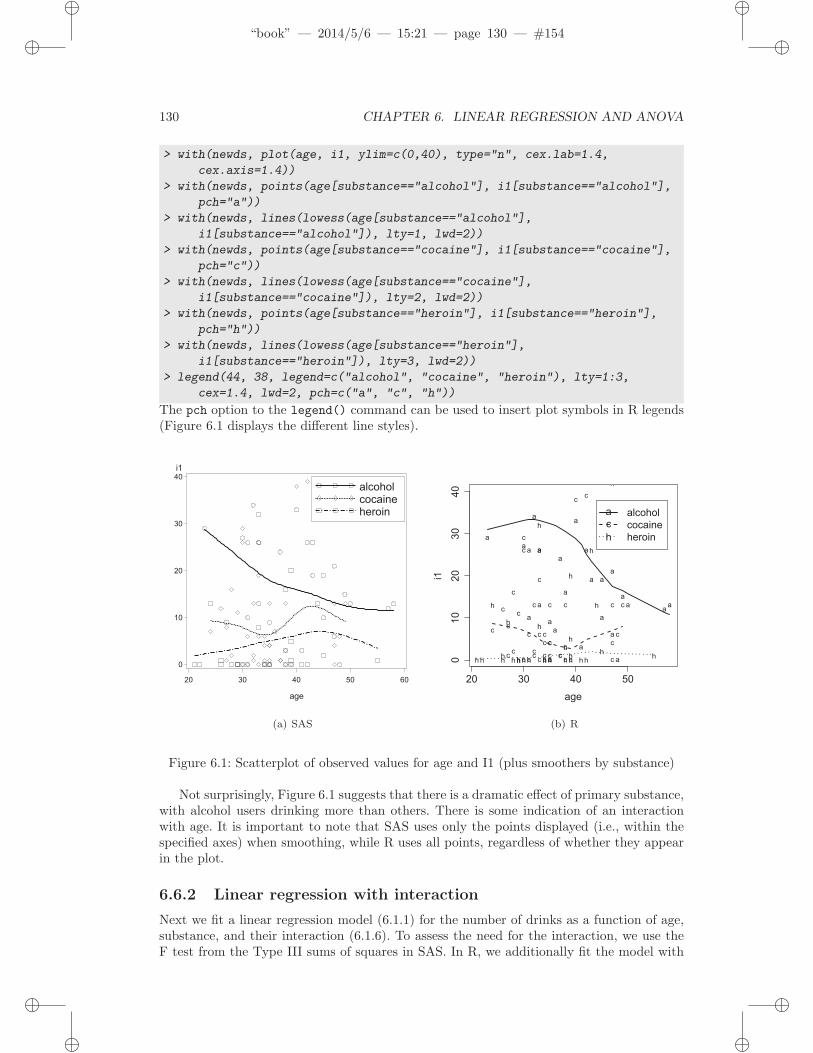
As a first step to help guide fitting a linear regression, we create a scatterplot (8.3.1)displaying the relationship between age and the number of alcoholic drinks consumed inthe period before entering detox (variable name: i1), as well as primary substance of abuse(alcohol, cocaine, or heroin).

Figure 6.1 displays a scatterplot of observed values for i1 (along with separate smoothfits by primary substance). To improve legibility, the plotting region is restricted to thosewith number of drinks between 0 and 40 (see plotting limits, 9.2.9).

axis1 order = (0 to 40 by 10) minor=none;

axis2 minor=none;

legend1 label=none value=(h=1.5) shape=symbol(10,1.2)

down=3 position=(top right inside) frame mode=protect;

symbol1 v=circle i=sm70s c=black l=1 h=1.1 w=5;

symbol2 v=diamond i=sm70s c=black l=33 h=1.1 w=5;

symbol3 v=square i=sm70s c=black l=8 h=1.1 w=5;

proc gplot data=help;

plot i1*age = substance / vaxis=axis1 haxis=axis2 legend=legend1;

run; quit;

✐

✐

“book” — 2014/5/6 — 15:21 — page 130 — #154✐

✐

✐

✐

✐

✐


> with(newds, plot(age, i1, ylim=c(0,40), type="n", cex.lab=1.4,

cex.axis=1.4))

> with(newds, points(age[substance=="alcohol"], i1[substance=="alcohol"],

pch="a"))

> with(newds, lines(lowess(age[substance=="alcohol"],

i1[substance=="alcohol"]), lty=1, lwd=2))

> with(newds, points(age[substance=="cocaine"], i1[substance=="cocaine"],

pch="c"))

> with(newds, lines(lowess(age[substance=="cocaine"],

i1[substance=="cocaine"]), lty=2, lwd=2))

> with(newds, points(age[substance=="heroin"], i1[substance=="heroin"],

pch="h"))

> with(newds, lines(lowess(age[substance=="heroin"],

i1[substance=="heroin"]), lty=3, lwd=2))

> legend(44, 38, legend=c("alcohol", "cocaine", "heroin"), lty=1:3,

cex=1.4, lwd=2, pch=c("a", "c", "h"))

The pch option to the legend() command can be used to insert plot symbols in R legends(Figure 6.1 displays the different line styles).

i1

0

10

20

30

40

age

20 30 40 50 60

alcoholcocaineheroin

(a) SAS

20 30 40 50

010

20

30

40

age

i1

a

a

a

a

a

aa

a

a

a

aa

aa

a a

a

a

a

aa

a a

a

a

a

c

c

cc

cc

cc

c

c

c

c

c

cc

c

c

c

c

c

c

c

c

cc

c

c

c

c

c

c

c

c

c

c

c

cc

c

ch

hh

h

h hhh

h

h

h

h h

h

h

h

h

hh

hhh

h

hh h

h

h

h

h

a

c

h

alcohol

cocaine

heroin

(b) R

Figure 6.1: Scatterplot of observed values for age and I1 (plus smoothers by substance)

Not surprisingly, Figure 6.1 suggests that there is a dramatic effect of primary substance,with alcohol users drinking more than others. There is some indication of an interactionwith age. It is important to note that SAS uses only the points displayed (i.e., within thespecified axes) when smoothing, while R uses all points, regardless of whether they appearin the plot.

6.6.2 Linear regression with interaction

Next we fit a linear regression model (6.1.1) for the number of drinks as a function of age,substance, and their interaction (6.1.6). To assess the need for the interaction, we use theF test from the Type III sums of squares in SAS. In R, we additionally fit the model with

✐

✐

“book” — 2014/5/6 — 15:21 — page 131 — #155✐

✐

✐

✐

✐

✐

6.6. EXAMPLES 131

no interaction and use the anova() function to compare the models (the drop1() functioncould also be used). To save space, some results of proc glm have been suppressed usingthe ods select statement (see A.7).

options ls=74; /* reduces width of output to make it fit in gray area */

ods select overallanova modelanova parameterestimates;

proc glm data=help;

class substance;

model i1 = age substance age * substance / solution;

output out=helpout cookd=cookd_ch4 dffits=dffits_ch4

student=sresids_ch4 residual=resid_ch4

predicted=pred_ch4 h=lev_ch4;

run; quit;

ods select all;

The GLM Procedure

Dependent Variable: i1 i1

Sum of

Source DF Squares Mean Square F Value Pr > F

Model 5 12275.17570 2455.03514 9.99 <.0001

Error 101 24815.36635 245.69670

Corrected Total 106 37090.54206

The GLM Procedure


Source DF Type I SS Mean Square F Value Pr > F

age 1 384.75504 384.75504 1.57 0.2137

substance 2 10509.56444 5254.78222 21.39 <.0001

age*substance 2 1380.85622 690.42811 2.81 0.0649

Source DF Type III SS Mean Square F Value Pr > F

age 1 27.157727 27.157727 0.11 0.7402

substance 2 3318.992822 1659.496411 6.75 0.0018

age*substance 2 1380.856222 690.428111 2.81 0.0649

✐

✐

“book” — 2014/5/6 — 15:21 — page 132 — #156✐

✐

✐

✐

✐

✐


The GLM Procedure


Standard

Parameter Estimate Error t Value Pr > |t|

Intercept -7.77045212 B 12.87885672 -0.60 0.5476

age 0.39337843 B 0.36221749 1.09 0.2801

substance alcohol 64.88044165 B 18.48733701 3.51 0.0007

substance cocaine 13.02733169 B 19.13852222 0.68 0.4976

substance heroin 0.00000000 B . . .

age*substance alcohol -1.11320795 B 0.49135408 -2.27 0.0256

age*substance cocaine -0.27758561 B 0.53967749 -0.51 0.6081

age*substance heroin 0.00000000 B . . .

> options(show.signif.stars=FALSE)

> lm1 = lm(i1 ~ sub * age, data=newds)

> lm2 = lm(i1 ~ sub + age, data=newds)

> anova(lm2, lm1)

Analysis of Variance Table

Model 1: i1 ~ sub + age

Model 2: i1 ~ sub * age

Res.Df RSS Df Sum of Sq F Pr(>F)

1 103 26196

2 101 24815 2 1381 2.81 0.065

> summary.aov(lm1)

Df Sum Sq Mean Sq F value Pr(>F)

sub 2 10810 5405 22.00 1.2e-08

age 1 84 84 0.34 0.559

sub:age 2 1381 690 2.81 0.065

Residuals 101 24815 246There is some indication of a borderline significant interaction between age and substancegroup (p=0.065).

In SAS, the ods output statement can be used to save any printed result as a SASdataset. In the following code, all printed output from proc glm is suppressed, but theparameter estimates are saved as a SAS dataset, then printed using proc print. In addition,various diagnostics are saved via the the output statement.ods select none;

ods output parameterestimates=helpmodelanova;

proc glm data=help;

class substance;

model i1 = age|substance / solution;

output out=helpout cookd=cookd_ch4 dffits=dffits_ch4

student=sresids_ch4 residual=resid_ch4

predicted=pred_ch4 h=lev_ch4;

run; quit;

ods select all;

✐

✐

“book” — 2014/5/6 — 15:21 — page 133 — #157✐

✐

✐

✐

✐

✐

6.6. EXAMPLES 133

proc print data=helpmodelanova;

var parameter estimate stderr tvalue probt;

format _numeric_ 6.3;

run;

Obs Parameter Estimate StdErr tValue Probt

1 Intercept -7.770 12.879 -0.603 0.548

2 age 0.393 0.362 1.086 0.280

3 substance alcohol 64.880 18.487 3.509 0.001

4 substance cocaine 13.027 19.139 0.681 0.498

5 substance heroin 0.000 . . .

6 age*substance alcohol -1.113 0.491 -2.266 0.026

7 age*substance cocaine -0.278 0.540 -0.514 0.608

8 age*substance heroin 0.000 . . .

In R, the summary() function provides similar information.

> summary(lm1)

Call:

lm(formula = i1 ~ sub * age, data = newds)

Residuals:

Min 1Q Median 3Q Max

-31.92 -8.25 -4.18 3.58 49.88

Coefficients:

Estimate Std. Error t value Pr(>|t|)

(Intercept) -7.770 12.879 -0.60 0.54763

subalcohol 64.880 18.487 3.51 0.00067

subcocaine 13.027 19.139 0.68 0.49763

age 0.393 0.362 1.09 0.28005

subalcohol:age -1.113 0.491 -2.27 0.02561

subcocaine:age -0.278 0.540 -0.51 0.60813

Residual standard error: 15.7 on 101 degrees of freedom

Multiple R-squared: 0.331, Adjusted R-squared: 0.298

F-statistic: 9.99 on 5 and 101 DF, p-value: 8.67e-08

> confint(lm1)

2.5 % 97.5 %

(Intercept) -33.319 17.778

subalcohol 28.207 101.554

subcocaine -24.938 50.993

age -0.325 1.112

subalcohol:age -2.088 -0.138

subcocaine:age -1.348 0.793

It may also be useful to produce the table in LATEX format. In SAS, we can do this usingthe latex destination for the ODS system. When compiled, the resulting table is displayedin Figure 6.2.

✐

✐

“book” — 2014/5/6 — 15:21 — page 134 — #158✐

✐

✐

✐

✐

✐


ods latex file="c:\book\table.tex" style=styles.printer;

proc print data = helpmodelanova; run;

ods latex close;

Figure 6.2: SAS table produced with latex destination in ODS

In R, we can use the xtable package to display the regression results in LATEX, as shownin Table 6.1.> library(xtable)

> lmtab = xtable(lm1, digits=c(0,3,3,2,4), label="better",

caption="Formatted results using the {\\tt xtable} package")

> print(lmtab) # output the LaTeX

Table 6.1: Formatted results using the xtable packageEstimate Std. Error t value Pr(>|t|)

(Intercept) -7.770 12.879 -0.60 0.5476subalcohol 64.880 18.487 3.51 0.0007subcocaine 13.027 19.139 0.68 0.4976

age 0.393 0.362 1.09 0.2801subalcohol:age -1.113 0.491 -2.27 0.0256subcocaine:age -0.278 0.540 -0.51 0.6081

There are many quantities of interest stored in the linear model object lm1, and these canbe viewed or extracted for further use.> names(summary(lm1))

[1] "call" "terms" "residuals" "coefficients"

[5] "aliased" "sigma" "df" "r.squared"

[9] "adj.r.squared" "fstatistic" "cov.unscaled"

> summary(lm1)$sigma

[1] 15.7

> names(lm1)

[1] "coefficients" "residuals" "effects" "rank"

[5] "fitted.values" "assign" "qr" "df.residual"

[9] "contrasts" "xlevels" "call" "terms"

[13] "model"

✐

✐

“book” — 2014/5/6 — 15:21 — page 135 — #159✐

✐

✐

✐

✐

✐

6.6. EXAMPLES 135

> coef(lm1)

(Intercept) subalcohol subcocaine age subalcohol:age

-7.770 64.880 13.027 0.393 -1.113

subcocaine:age

-0.278

> vcov(lm1)

(Intercept) subalcohol subcocaine age subalcohol:age

(Intercept) 165.86 -165.86 -165.86 -4.548 4.548

subalcohol -165.86 341.78 165.86 4.548 -8.866

subcocaine -165.86 165.86 366.28 4.548 -4.548

age -4.55 4.55 4.55 0.131 -0.131

subalcohol:age 4.55 -8.87 -4.55 -0.131 0.241

subcocaine:age 4.55 -4.55 -10.13 -0.131 0.131

subcocaine:age

(Intercept) 4.548

subalcohol -4.548

subcocaine -10.127

age -0.131

subalcohol:age 0.131

subcocaine:age 0.291

6.6.3 Regression diagnostics

Assessing the model is an important part of any analysis. We begin by examining theresiduals (6.3.2). First, we calculate the quantiles of their distribution (5.1.4), then displaythe smallest residual.options ls=74;

proc means data=helpout min q1 median q3 max maxdec=2;

var resid_ch4;

run;

The MEANS Procedure

Analysis Variable : resid_ch4

Lower Upper

Minimum Quartile Median Quartile Maximum

------------------------------------------------------------------------

-31.92 -8.31 -4.18 3.69 49.88

------------------------------------------------------------------------

> newds = transform(newds, pred = fitted(lm1))

> newds = transform(newds, resid = residuals(lm1))

> with(newds, quantile(resid))

0% 25% 50% 75% 100%

-31.92 -8.25 -4.18 3.58 49.88We could examine the output, then condition to find the value of the residual that is lessthan −31. Instead the dataset can be sorted so the smallest observation is first and thenprint one observation.

✐

✐

“book” — 2014/5/6 — 15:21 — page 136 — #160✐

✐

✐

✐

✐

✐


proc sort data=helpout;

by resid_ch4;

run;

proc print data=helpout (obs=1);

var id age i1 substance pred_ch4 resid_ch4;

run;

resid_

Obs id age i1 substance pred_ch4 ch4

1 325 35 0 alcohol 31.9160 -31.9160One way to print the largest value is to sort the dataset in the reverse order (2.3.10), thenprint just the first observation.proc sort data=helpout;

by descending resid_ch4;

run;

proc print data=helpout (obs=1);

var id age i1 substance pred_ch4 resid_ch4;

run;

resid_

Obs id age i1 substance pred_ch4 ch4

1 9 50 71 alcohol 21.1185 49.8815

> tmpds = with(newds,

data.frame(id, age, i1, sub, pred, resid, rstandard(lm1)))

> subset(tmpds, resid==max(resid))

id age i1 sub pred resid rstandard.lm1.

9 9 50 71 alcohol 21.1 49.9 3.32Graphical tools are one of the best ways to examine residuals. Figure 6.3 displays the defaultdiagnostic plots (6.3) from the model (for R) and the Q-Q plot generated from the saveddiagnostics (for SAS).

Sometimes in SAS it is necessary to clear out old graphics settings. This is easiest to dowith the goptions reset=all statement (9.2.8).

goptions reset=all;

ods select univar;

proc univariate data=helpout;

qqplot resid_ch4 / normal(mu=est sigma=est color=black);

run;

ods select all;

> oldpar = par(mfrow=c(2, 2), mar=c(4, 4, 2, 2)+.1)

> plot(lm1)

> par(oldpar)

In SAS, we get assorted diagnostic plots by default, but here we demonstrate a manualapproach using the previously saved diagnostics. Figure 6.4 displays the empirical densityof the standardized residuals, along with an overlaid normal density. The assumption thatthe residuals are approximately Gaussian does not appear to be tenable.

✐

✐

“book” — 2014/5/6 — 15:21 — page 137 — #161✐

✐

✐

✐

✐

✐

6.6. EXAMPLES 137

-3 -2 -1 0 1 2 3

-40

-20

0

20

40

60

resid

_ch4

Normal Quantiles

(a) SAS

0 10 20 30 40

−40

−20

020

40

60

Fitted values

Resid

uals

Residuals vs Fitted

9320

295

−2 −1 0 1 2

−2

−1

01

23

Theoretical Quantiles

Sta

ndard

ized r

esid

uals

Normal Q−Q

9320

295

0 10 20 30 40

0.0

0.5

1.0

1.5

Fitted valuesS

tandard

ized

resid

uals

Scale−Location9

320

295

0.00 0.10 0.20

−2

−1

01

23

4

Leverage

Sta

ndard

ized r

esid

uals

Cook's distance

0.5

Residuals vs Leverage

9

213

225

(b) R

Figure 6.3: Q-Q plot from SAS, default diagnostics from R

-2.8 -2.0 -1.2 -0.4 0.4 1.2 2.0 2.8 3.6 4.4

0

10

20

30

40

50

60

70

Perc

ent

Standardized residuals

(a) SAS

standardized residuals

Density

−2 −1 0 1 2 3

0.0

0.2

0.4

0.6

0.8

(b) R

Figure 6.4: Empirical density of residuals, with superimposed normal density

axis1 label=("Standardized residuals");

ods select "Histogram 1";

proc univariate data=helpout;

var sresids_ch4;

histogram sresids_ch4 / normal(mu=est sigma=est color=black)

kernel(color=black) haxis=axis1;

run;

ods select all;

✐

✐

“book” — 2014/5/6 — 15:21 — page 138 — #162✐

✐

✐

✐

✐

✐


> library(MASS)

> std.res = rstandard(lm1)

> hist(std.res, breaks=seq(-2.5, 3.5, by=.5), main="",

xlab="standardized residuals", col="gray80", freq=FALSE)

> lines(density(std.res), lwd=2)

> xvals = seq(from=min(std.res), to=max(std.res), length=100)

> lines(xvals, dnorm(xvals, mean(std.res), sd(std.res)), lty=2)

The residual plots indicate some potentially important departures from model assumptions,and further exploration should be undertaken.

6.6.4 Fitting the regression model separately for each value of an-

other variable

One common task is to perform identical analyses in several groups. Here, as an example,we consider separate linear regressions for each substance abuse group. In SAS, we showonly the parameter estimates, using ODS.ods select none;

proc sort data=help;

by substance;

run;

ods output parameterestimates=helpsubstparams;

proc glm data=help;

by substance;

model i1 = age / solution;

run;

ods select all;

options ls=74;

proc print data=helpsubstparams;

run;

Obs substance Dependent Parameter Estimate StdErr tValue Probt

1 alcohol i1 Intercept 57.10998953 18.00474934 3.17 0.0032

2 alcohol i1 age -0.71982952 0.45069028 -1.60 0.1195

3 cocaine i1 Intercept 5.25687957 11.52989056 0.46 0.6510

4 cocaine i1 age 0.11579282 0.32582541 0.36 0.7242

5 heroin i1 Intercept -7.77045212 8.59729637 -0.90 0.3738

6 heroin i1 age 0.39337843 0.24179872 1.63 0.1150

For R, a matrix of the correct size is created, then a for loop is run for each unique valueof the grouping variable.

✐

✐

“book” — 2014/5/6 — 15:21 — page 139 — #163✐

✐

✐

✐

✐

✐

6.6. EXAMPLES 139

> uniquevals = unique(newds$substance)

> numunique = length(uniquevals)

> formula = as.formula(i1 ~ age)

> p = length(coef(lm(formula, data=newds)))

> res = matrix(rep(0, numunique*p), p, numunique)

> for (i in 1:length(uniquevals)) {

res[,i] = coef(lm(formula,

data=subset(newds, substance==uniquevals[i])))

}

> rownames(res) = c("intercept","slope")

> colnames(res) = uniquevals

> res

heroin cocaine alcohol

intercept -7.770 5.257 57.11

slope 0.393 0.116 -0.72

6.6.5 Two-way ANOVA

Is there a statistically significant association between gender and substance abuse groupwith depressive symptoms? In SAS, we can make an interaction plot (8.5.2) by hand, asbelow, or proc glm will make a similar one automatically.

libname k 'c:/book';

proc sort data=k.help;

by substance female;

run;

ods select none;

proc means data=k.help;

by substance female;

var cesd;

output out=helpmean mean=;

run;

ods select all;

axis1 minor=none;

symbol1 i=j v=none l=1 c=black w=5;

symbol2 i=j v=none l=2 c=black w=5;

proc gplot data=helpmean;

plot cesd*substance = female / haxis=axis1 vaxis=axis1;

run; quit;

R has a function interaction.plot() to carry out this task. Figure 6.5 displays an inter-action plot for CESD as a function of substance group and gender.

> ds = transform(ds, genf = as.factor(ifelse(female, "F", "M")))

> with(ds, interaction.plot(substance, genf, cesd,

xlab="substance", las=1, lwd=2))

There are indications of large effects of gender and substance group, but little suggestion ofinteraction between the two. The same conclusion is reached in Figure 6.6, which displaysboxplots by substance group and gender.

✐

✐

“book” — 2014/5/6 — 15:21 — page 140 — #164✐

✐

✐

✐

✐

✐


CESD

28

29

30

31

32

33

34

35

36

37

38

39

40

41

SUBSTANCE

alcohol cocaine heroin

FEMALE 0 1

(a) SAS

28

30

32

34

36

38

40

substance

mean o

f c

esd

alcohol cocaine heroin

genf

F

M

(b) R

Figure 6.5: Interaction plot of CESD as a function of substance group and gender

alcohol cocaine heroin alcohol cocaine heroin

0

20

40

60

CESD

SUBSTANCE

F M

(a) SAS

Alc.F Coc.F Her.F Alc.M Coc.M Her.M

010

20

30

40

50

60

(b) R

Figure 6.6: Boxplot of CESD as a function of substance group and gender

data h2; set k.help;

if female eq 1 then sex='F';

else sex='M';

run;

proc sort data=h2; by sex; run;

symbol1 v='x' c=black;

proc boxplot data=h2;

plot cesd * substance(sex) / notches boxwidthscale=1;

run;

✐

✐

“book” — 2014/5/6 — 15:21 — page 141 — #165✐

✐

✐

✐

✐

✐

6.6. EXAMPLES 141

> library(memisc)

> ds = transform(ds, subs = cases(

"Alc" = substance=="alcohol",

"Coc" = substance=="cocaine",

"Her" = substance=="heroin"))

> boxout = with(ds,

boxplot(cesd ~ subs + genf, notch=TRUE, varwidth=TRUE,

col="gray80"))

> boxmeans = with(ds, tapply(cesd, list(subs, genf), mean))

> points(seq(boxout$n), boxmeans, pch=4, cex=2)

The width of each box is proportional to the size of the sample, with the notches denotingconfidence intervals for the medians and X’s marking the observed means. Next, we proceedto formally test whether there is a significant interaction through a two-way analysis ofvariance (6.1.8). In SAS, the Type III sums of squares table can be used to assess theinteraction; we restrict output to this table to save space. In R we fit models with andwithout an interaction, and then compare the results. We also construct the likelihood ratiotest manually.options ls=74;

ods select modelanova;

proc glm data=k.help;

class female substance;

model cesd = female substance female*substance / ss3;

run;

The GLM Procedure

Dependent Variable: CESD

Source DF Type III SS Mean Square F Value Pr > F

FEMALE 1 2463.232928 2463.232928 16.84 <.0001

SUBSTANCE 2 2540.208432 1270.104216 8.69 0.0002

FEMALE*SUBSTANCE 2 145.924987 72.962494 0.50 0.6075

> aov1 = aov(cesd ~ sub * genf, data=ds)

> aov2 = aov(cesd ~ sub + genf, data=ds)

> resid = residuals(aov2)

> anova(aov2, aov1)

Analysis of Variance Table

Model 1: cesd ~ sub + genf

Model 2: cesd ~ sub * genf

Res.Df RSS Df Sum of Sq F Pr(>F)

1 449 65515

2 447 65369 2 146 0.5 0.61

✐

✐

“book” — 2014/5/6 — 15:21 — page 142 — #166✐

✐

✐

✐

✐

✐


> options(digits=6)

> logLik(aov1)

'log Lik.' -1768.92 (df=7)

> logLik(aov2)

'log Lik.' -1769.42 (df=5)

> lldiff = logLik(aov1)[1] - logLik(aov2)[1]

> lldiff

[1] 0.505055

> 1 - pchisq(2*lldiff, df=2)

[1] 0.603472

> options(digits=3)

> summary(aov2)

Df Sum Sq Mean Sq F value Pr(>F)

sub 2 2704 1352 9.27 0.00011

genf 1 2569 2569 17.61 3.3e-05

Residuals 449 65515 146There is little evidence (p=0.61) of an interaction, so this term can be dropped. For SAS,this means estimating the reduced model.

options ls=74; /* stay in gray box */

ods select overallanova parameterestimates;



model cesd = female substance / ss3 solution;

run;

The GLM Procedure


Sum of

Source DF Squares Mean Square F Value Pr > F

Model 3 5273.13263 1757.71088 12.05 <.0001

Error 449 65515.35744 145.91394

Corrected Total 452 70788.49007

✐

✐

“book” — 2014/5/6 — 15:21 — page 143 — #167✐

✐

✐

✐

✐

✐

6.6. EXAMPLES 143

The GLM Procedure


Standard


Intercept 39.13070331 B 1.48571047 26.34 <.0001

FEMALE 0 -5.61922564 B 1.33918653 -4.20 <.0001

FEMALE 1 0.00000000 B . . .

SUBSTANCE alcohol -0.28148966 B 1.41554315 -0.20 0.8425

SUBSTANCE cocaine -5.60613722 B 1.46221461 -3.83 0.0001

SUBSTANCE heroin 0.00000000 B . . .The model was already fit in R to allow assessment of the interaction.> aov2

Call:

aov(formula = cesd ~ sub + genf, data = ds)

Terms:

sub genf Residuals

Sum of Squares 2704 2569 65515

Deg. of Freedom 2 1 449

Residual standard error: 12.1

Estimated effects may be unbalanced

If results with the same referent categories used by SAS are desired, the default R designmatrix (see 6.1.4) can be changed and the model re-fit.

> contrasts(ds$sub) = contr.SAS(3)

> aov3 = lm(cesd ~ sub + genf, data=ds)

> summary(aov3)

Call:

lm(formula = cesd ~ sub + genf, data = ds)

Residuals:

Min 1Q Median 3Q Max

-32.13 -8.85 1.09 8.48 27.09

Coefficients:

Estimate Std. Error t value Pr(>|t|)

(Intercept) 33.52 1.38 24.22 < 2e-16

sub1 5.61 1.46 3.83 0.00014

sub2 5.32 1.34 3.98 8.1e-05

genfM -5.62 1.34 -4.20 3.3e-05

Residual standard error: 12.1 on 449 degrees of freedom

Multiple R-squared: 0.0745, Adjusted R-squared: 0.0683

F-statistic: 12 on 3 and 449 DF, p-value: 1.35e-07

The AIC criteria (7.8.3) can also be used to compare models. In SAS it is available in proc

reg and proc mixed. Here we use proc mixed, omitting other output.

✐

✐

“book” — 2014/5/6 — 15:21 — page 144 — #168✐

✐

✐

✐

✐

✐


ods select fitstatistics;

proc mixed data=k.help method=ml;


model cesd = female|substance;

run; quit;

The Mixed Procedure

Fit Statistics

-2 Log Likelihood 3537.8

AIC (smaller is better) 3551.8

AICC (smaller is better) 3552.1

BIC (smaller is better) 3580.6

ods select fitstatistics;

proc mixed data=k.help method=ml;


model cesd = female substance;

run; quit;

ods select all;

The Mixed Procedure

Fit Statistics

-2 Log Likelihood 3538.8

AIC (smaller is better) 3548.8

AICC (smaller is better) 3549.0

BIC (smaller is better) 3569.4

> AIC(aov1)

[1] 3552

> AIC(aov2)

[1] 3549

The AIC criterion also suggests that the model without the interaction is most appropriate.

6.6.6 Multiple comparisons

We can also carry out multiple comparison (6.2.4) procedures to test each of the pairwisedifferences between substance abuse groups. In SAS this utilizes the lsmeans statementwithin proc glm.ods select diff lsmeandiffcl lsmlines diffplot;


class substance;

model cesd = substance;

lsmeans substance / pdiff adjust=tukey cl lines;

run; quit;

ods select all;

✐

✐

“book” — 2014/5/6 — 15:21 — page 145 — #169✐

✐

✐

✐

✐

✐

6.6. EXAMPLES 145

The GLM Procedure

Least Squares Means

Adjustment for Multiple Comparisons: Tukey-Kramer

Least Squares Means for effect SUBSTANCE

Pr > |t| for H0: LSMean(i)=LSMean(j)


i/j 1 2 3

1 0.0009 0.9362

2 0.0009 0.0008

3 0.9362 0.0008

The GLM Procedure

Least Squares Means


Least Squares Means for Effect SUBSTANCE

Difference Simultaneous 95%

Between Confidence Limits for

i j Means LSMean(i)-LSMean(j)

1 2 4.951829 1.753296 8.150362

1 3 -0.498086 -3.885335 2.889162

2 3 -5.449915 -8.950037 -1.949793

The GLM Procedure

Least Squares Means


Tukey-Kramer Comparison Lines for Least Squares Means of SUBSTANCE

LS-means with the same letter are not significantly different.

CESD LSMEAN

LSMEAN SUBSTANCE Number

A 34.87097 heroin 3

A

A 34.37288 alcohol 1

B 29.42105 cocaine 2The above output demonstrates the results of the lines option using the lsmeans state-ment. The letter A shown on the left connecting the heroin and alcohol substances im-plies that there is not a statistically significant difference between these two groups. Sincethe cocaine substance has the letter B and no other group has one, the cocaine group issignificantly different from each of the other groups. If instead the cocaine and alcohol

substances both had a letter B attached, while the heroin and alcohol substances retainedthe letter A they have in the actual output, only the heroin and cocaine groups would differsignificantly, while the alcohol group would differ from neither. This presentation becomes

✐

✐

“book” — 2014/5/6 — 15:21 — page 146 — #170✐

✐

✐

✐

✐

✐


CESD Comparisons for SUBSTANCE

SignificantNot significant

Differences for alpha=0.05 (Tukey-Kramer Adjustment)

alcoholcocaine heroin

alcohol

cocaine

heroin

28 30 32 34 36

28

30

32

34

36

(a) SAS

−8 −6 −4 −2 0 2

cocain

e−

alc

ohol

cocain

e−

hero

inalc

ohol−

hero

in

95% family−wise confidence level

Differences in mean levels of sub

(b) R

Figure 6.7: Pairwise comparisons

particularly useful as the number of groups increases. A graphical version called a diffplotis also produced; it is shown in Figure 6.7.

In R, we use the TukeyHSD() function.

> mult = TukeyHSD(aov(cesd ~ sub, data=ds), "sub")

> mult

Tukey multiple comparisons of means

95% family-wise confidence level

Fit: aov(formula = cesd ~ sub, data = ds)

$sub

diff lwr upr p adj

alcohol-heroin -0.498 -3.89 2.89 0.936

cocaine-heroin -5.450 -8.95 -1.95 0.001

cocaine-alcohol -4.952 -8.15 -1.75 0.001The alcohol group and heroin group both have significantly higher CESD scores than thecocaine group, but the alcohol and heroin groups do not significantly differ from each other(95% CI for the difference ranges from −3.9 to 2.9). Figure 6.7 provides a graphical displayof the pairwise comparisons.

> plot(mult)

6.6.7 Contrasts

We can also fit contrasts (6.2.3) to test hypotheses involving multiple parameters. In thiscase, we can compare the CESD scores for the alcohol and heroin groups to the cocainegroup. In SAS, to allow checking the contrast, we use the e option to the estimate state-ment.

✐

✐

“book” — 2014/5/6 — 15:21 — page 147 — #171✐

✐

✐

✐

✐

✐

6.6. EXAMPLES 147

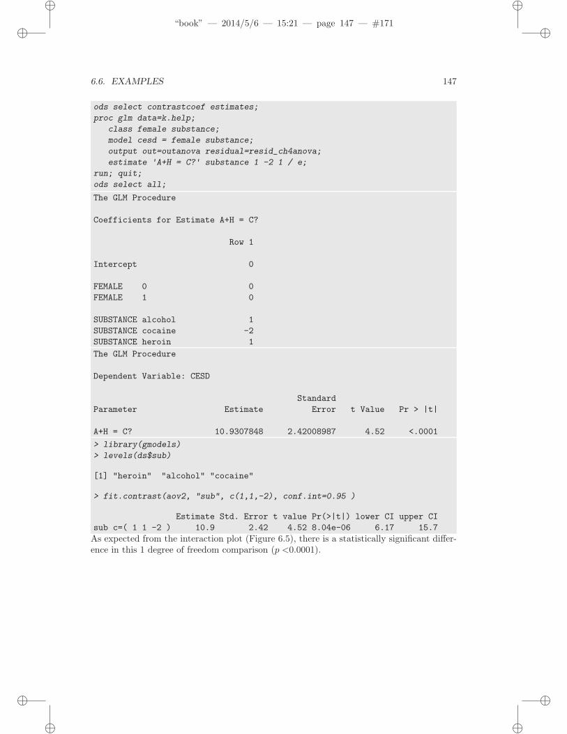
ods select contrastcoef estimates;



model cesd = female substance;

output out=outanova residual=resid_ch4anova;

estimate 'A+H = C?' substance 1 -2 1 / e;

run; quit;

ods select all;

The GLM Procedure

Coefficients for Estimate A+H = C?

Row 1

Intercept 0

FEMALE 0 0

FEMALE 1 0

SUBSTANCE alcohol 1

SUBSTANCE cocaine -2

SUBSTANCE heroin 1

The GLM Procedure


Standard


A+H = C? 10.9307848 2.42008987 4.52 <.0001

> library(gmodels)

> levels(ds$sub)

[1] "heroin" "alcohol" "cocaine"

> fit.contrast(aov2, "sub", c(1,1,-2), conf.int=0.95 )

Estimate Std. Error t value Pr(>|t|) lower CI upper CI

sub c=( 1 1 -2 ) 10.9 2.42 4.52 8.04e-06 6.17 15.7

As expected from the interaction plot (Figure 6.5), there is a statistically significant differ-ence in this 1 degree of freedom comparison (p <0.0001).

Documents

Linear regression and ANOVA - Amherst College · Linear regression and ANOVA Regression and analysis of variance form the basis of many investigations. In this chapter we describe