Linear regression / ANOVAstaff.pubhealth.ku.dk/~sr/MPH/slides/dag4.pdf · · 2017-05-05Linear regression / ANOVA Susanne Rosthøj ... One-way ANOVA In one-way ANOVA we ... therefore

u n i v e r s i t y o f c o p e n h a g e n d e p a r t m e n t o f b i o s t a t i s t i c s

Dag 4: Linear regression / ANOVA

Susanne Rosthøj

Section of BiostatisticsDepartment of Public HealthUniversity of Copenhagen

[email protected]


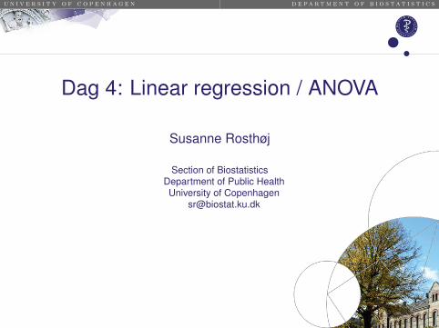
Regression models

The purpose with a regression analysis is to relate one outcomevariable to one or more explanatory variables.

The type of the outcome variable determines which kind of regressionmodel is relevant:

Outcome Model Effect0/1 (binary) logistic regression odds ratioQuantitative linear regression difference in meansSurvival time Cox (Poisson) regression hazard (rate) ratio

2 / 1


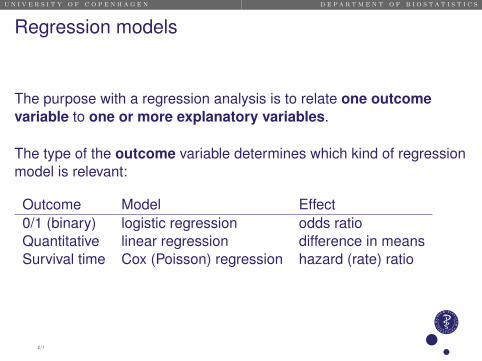
Linear regression model

The outcome Y has a normal distribution with

EY = a + b · XVarY = σ2

where X is a quanititative explanatory variable.

n independent observations Y1,Y2, . . . ,Yn.

We write

Yi = a + b · Xi + εi, with εi ∼ N (0, σ2) independent

ε is the residual error.

3 / 1


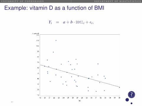
Example: vitamin D as a function of BMI

Yi = a + b · BMIi + εi,

4 / 1


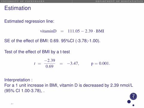
Estimation

Estimated regression line:

vitaminD = 111.05− 2.39 · BMI

SE of the effect of BMI: 0.69. 95%CI (-3.78;-1.00).

Test of the effect of BMI by a t-test

t = −2.390.69

= −3.47, p = 0.001.

Interpretation :For a 1 unit increase in BMI, vitamin D is decreased by 2.39 nmol/L(95% CI 1.00-3.78), .

5 / 1


Analysis in SAS

We use proc glm (General Linear Model):proc glm data=vitamin plots=DiagnosticsPanel;

model vitd = bmi / solution clparm;where country=4; * Irland;

run;

Discuss the output in the handout and find the numbers on theprevious slide.

6 / 1


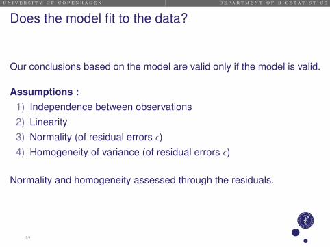
Does the model fit to the data?

Our conclusions based on the model are valid only if the model is valid.

Assumptions :1) Independence between observations2) Linearity3) Normality (of residual errors ε)4) Homogeneity of variance (of residual errors ε)

Normality and homogeneity assessed through the residuals.

7 / 1


Assessment of 2) Linearity

Extend the model :

Yi = a + b · BMIi + c · BMI2i + εi

A test of linearity : H0 : c = 0.

proc glm data=vitamin plots=DiagnosticsPanel;model vitd = bmi bmi*bmi / solution clparm;where country=4; * Irland;

run;

Conclude from handout: Is the linear model plausible?

8 / 1


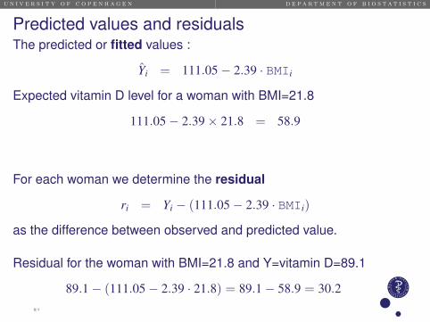
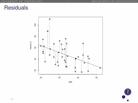
Predicted values and residualsThe predicted or fitted values :

Yi = 111.05− 2.39 · BMIi

Expected vitamin D level for a woman with BMI=21.8

111.05− 2.39× 21.8 = 58.9

For each woman we determine the residual

ri = Yi − (111.05− 2.39 · BMIi)

as the difference between observed and predicted value.

Residual for the woman with BMI=21.8 and Y=vitamin D=89.1

89.1− (111.05− 2.39 · 21.8) = 89.1− 58.9 = 30.29 / 1


Residuals

●

●

●

●

●

●

●●

●

●

●

●

●

●

●

●

●

●

●

●

●

●

●

●

●

●

●

●

●●

●

●

●

●

●

●

●

●

●

●

●

20 25 30 35

2040

6080

100

BMI

Vita

min

D●

10 / 1


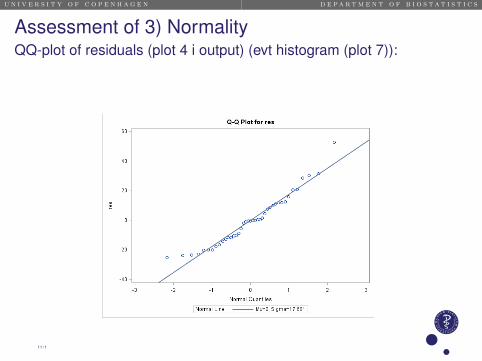
Assessment of 3) NormalityQQ-plot of residuals (plot 4 i output) (evt histogram (plot 7)):

11 / 1


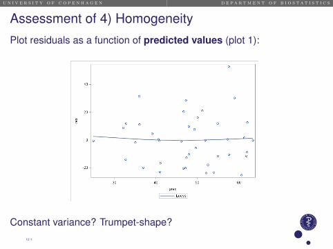
Assessment of 4) Homogeneity

Plot residuals as a function of predicted values (plot 1):

Constant variance? Trumpet-shape?12 / 1


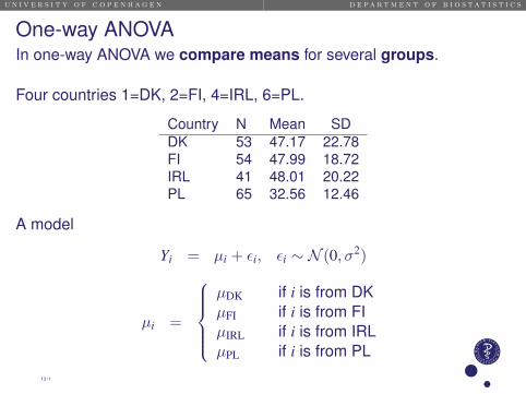
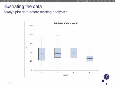
One-way ANOVAIn one-way ANOVA we compare means for several groups.

Four countries 1=DK, 2=FI, 4=IRL, 6=PL.

Country N Mean SDDK 53 47.17 22.78FI 54 47.99 18.72IRL 41 48.01 20.22PL 65 32.56 12.46

A model

Yi = µi + εi, εi ∼ N (0, σ2)

µi =

µDK if i is from DKµFI if i is from FIµIRL if i is from IRLµPL if i is from PL

13 / 1


An illustration of the model

Sampling distribution:

Mean

µ1 µ2 µ3 µ4

14 / 1


Illustrating the dataAlways plot data before starting analysis :

15 / 1


Useful formulation of mean structure

We are interested in quantifying the differences between the groups

µi =

µDK DKµFI FIµIRL IRLµPL PL

=

47.17 DK47.99 FI48.01 IRL32.56 PL

=

a DKa + b1 FIa + b2 IRLa + b3 IRL

=

47.17 DK47.17 + 0.82 FI47.17 + 0.84 IRL47.17− 14.60 PL

16 / 1


The overall test for associationHypothesis

H0 : µDK = µFI = µIRL = µPL

against HA : at least two means are different

Equivalently the hypothesis is

H0 : b1 = b2 = b3 = 0

against HA : either b1 6= 0, b2 6= 0 or b3 6= 0.

The test statistics follows an F-distribution with df=(k − 1, n− k) wheren = 213 is the total number of patients, k = 4 is the number of groups.

The test statistic compare the variance between the groups to thevariance within the groups, therefore an ANalysis Of VAriance(even though we are actually comparing means...).

17 / 1


One-way ANOVA in SAS

We again use proc glm:

proc glm data=vitamin;class country (ref=’1’);model vitd = country / solution clparm;

run;

18 / 1


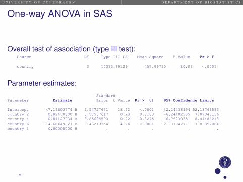
One-way ANOVA in SAS

Overall test of association (type III test):Source DF Type III SS Mean Square F Value Pr > F

country 3 10373.99129 457.99710 10.06 <.0001

Parameter estimates:

StandardParameter Estimate Error t Value Pr > |t| 95% Confidence Limits

Intercept 47.16603774 B 2.54727631 18.52 <.0001 42.14438954 52.18768593country 2 0.82470300 B 3.58567617 0.23 0.8183 -6.24402535 7.89343136country 4 0.84127934 B 3.85698593 0.22 0.8275 -6.76230351 8.44486218country 6 -14.60449927 B 3.43210354 -4.26 <.0001 -21.37047771 -7.83852084country 1 0.00000000 B . . . . .

19 / 1


Assumptions

Assumptions need to be checked:• the observations are independent (i.e. no siblings)• in each group, the distribution of the observations have to be

normal• the variances are the same in all groups.

20 / 1


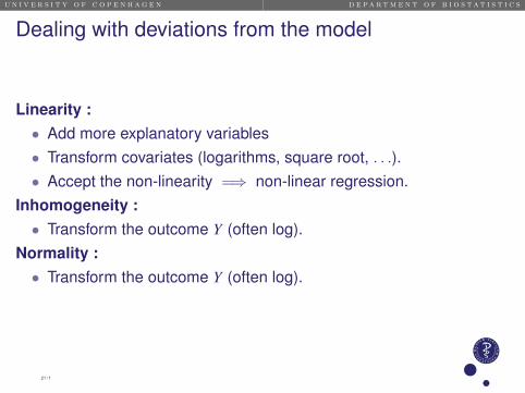
Dealing with deviations from the model

Linearity :• Add more explanatory variables• Transform covariates (logarithms, square root, . . .).• Accept the non-linearity =⇒ non-linear regression.

Inhomogeneity :• Transform the outcome Y (often log).

Normality :• Transform the outcome Y (often log).

21 / 1

Documents

Linear regression / ANOVAstaff.pubhealth.ku.dk/~sr/MPH/slides/dag4.pdf · · 2017-05-05Linear regression / ANOVA Susanne Rosthøj ... One-way ANOVA In one-way ANOVA we ... therefore