Repeated measuresa.k.a. within-subjects ANOVA

Repeated measures

Today’s goal: Teach you about within-subjects ANOVA, the test used to test the differences between more than two within-subjects conditions

Outline:

- The theory of within-subjects ANOVA

- Within-subjects ANOVA in R

- Within-subjects Factorial ANOVA in R

Within-subjects ANOVAthe theory

Within-subjects

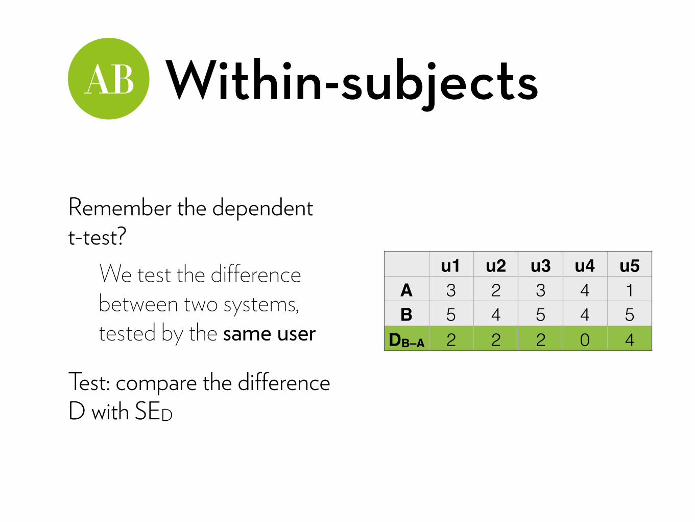
Remember the dependent t-test?

We test the difference between two systems, tested by the same user

Test: compare the difference D with SED

u1 u2 u3 u4 u5A 3 2 3 4 1B 5 4 5 4 5DB–A 2 2 2 0 4

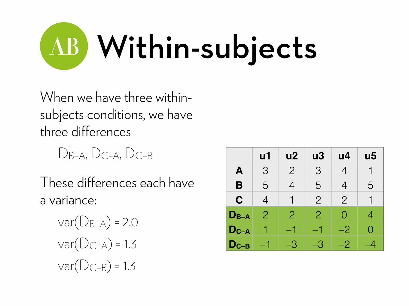
Within-subjectsWhen we have three within-subjects conditions, we have three differences

DB–A, DC–A, DC–B

These differences each have a variance:

var(DB–A) = 2.0 var(DC–A) = 1.3 var(DC–B) = 1.3

u1 u2 u3 u4 u5A 3 2 3 4 1B 5 4 5 4 5C 4 1 2 2 1DB–A 2 2 2 0 4DC–A 1 –1 –1 –2 0DC–B –1 –3 –3 –2 –4

Assumption

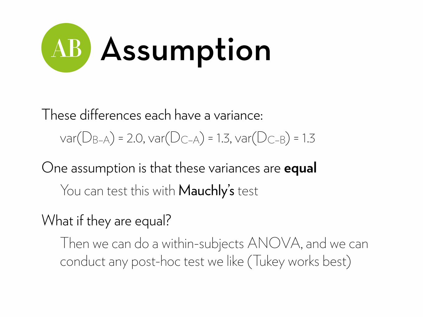
These differences each have a variance: var(DB–A) = 2.0, var(DC–A) = 1.3, var(DC–B) = 1.3

One assumption is that these variances are equal You can test this with Mauchly’s test

What if they are equal? Then we can do a within-subjects ANOVA, and we can conduct any post-hoc test we like (Tukey works best)

Assumption

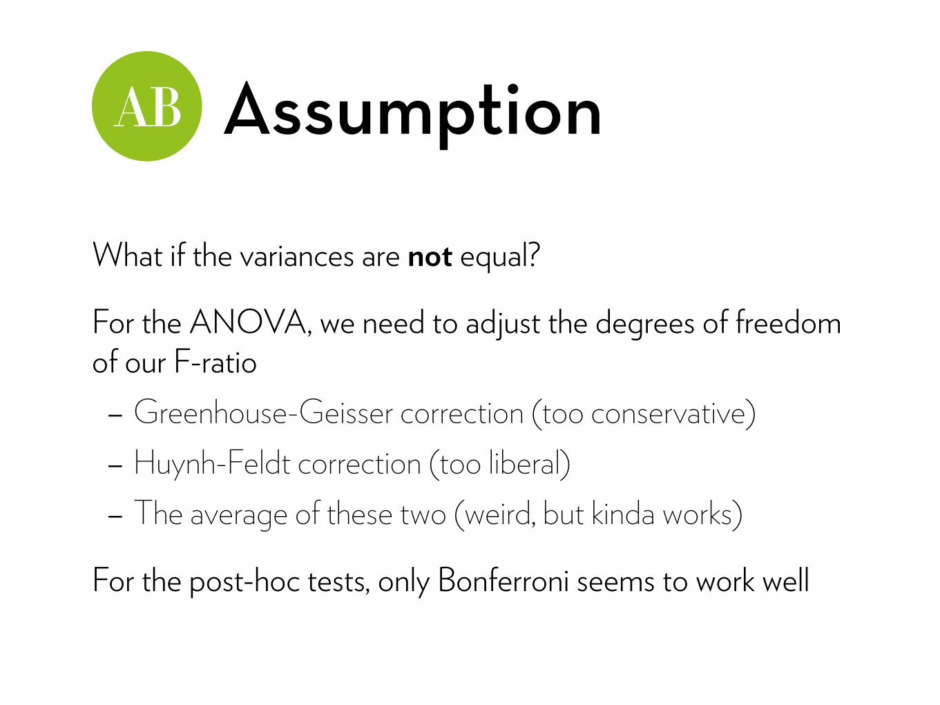
What if the variances are not equal?

For the ANOVA, we need to adjust the degrees of freedom of our F-ratio

- Greenhouse-Geisser correction (too conservative)

- Huynh-Feldt correction (too liberal)

- The average of these two (weird, but kinda works)

For the post-hoc tests, only Bonferroni seems to work well

Assumption

Or… we can run a multilevel linear model!

A multilevel linear model is a repeated measures version of linear regression

Remember, ANOVA and linear regression are kind of the same thing

Multilevel models far more flexible than the repeated measures ANOVA

We will learn all about them next week!

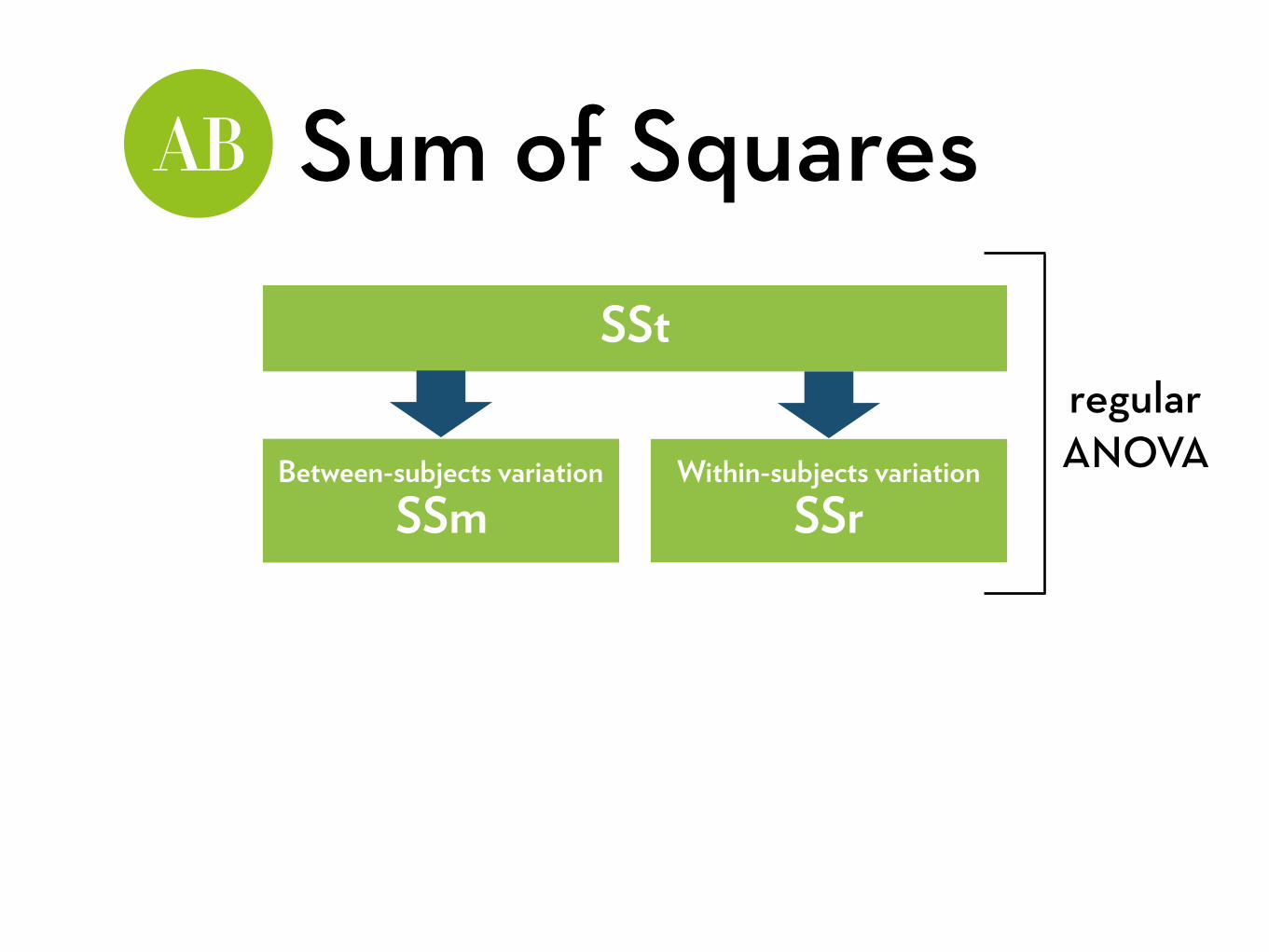
Sum of Squares

SSt

Between-subjects variation SSm

Within-subjects variation SSr

regular ANOVA

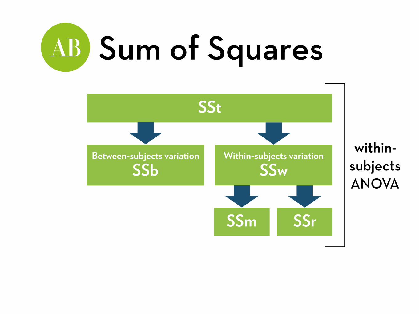
Sum of Squares

SSt

Between-subjects variation SSb

Within-subjects variation SSw

within-subjects ANOVA

SSm SSr

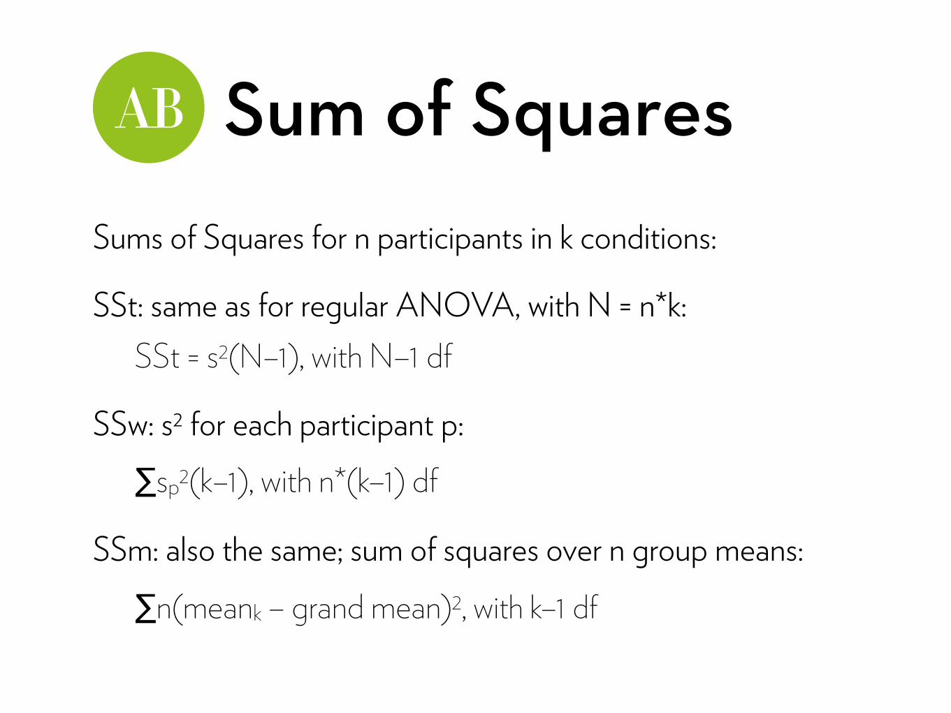
Sum of SquaresSums of Squares for n participants in k conditions:

SSt: same as for regular ANOVA, with N = n*k: SSt = s2(N–1), with N–1 df

SSw: s2 for each participant p:

∑sp2(k–1), with n*(k–1) df

SSm: also the same; sum of squares over n group means:

∑n(meank – grand mean)2, with k–1 df

Sum of Squares

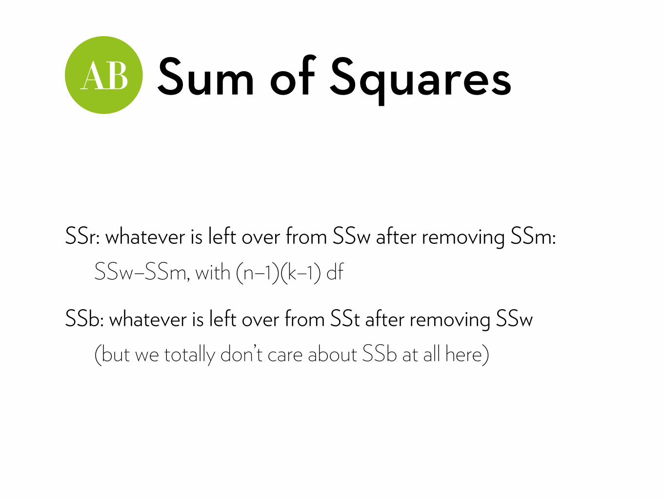
SSr: whatever is left over from SSw after removing SSm: SSw–SSm, with (n–1)(k–1) df

SSb: whatever is left over from SSt after removing SSw (but we totally don’t care about SSb at all here)

F-ratio

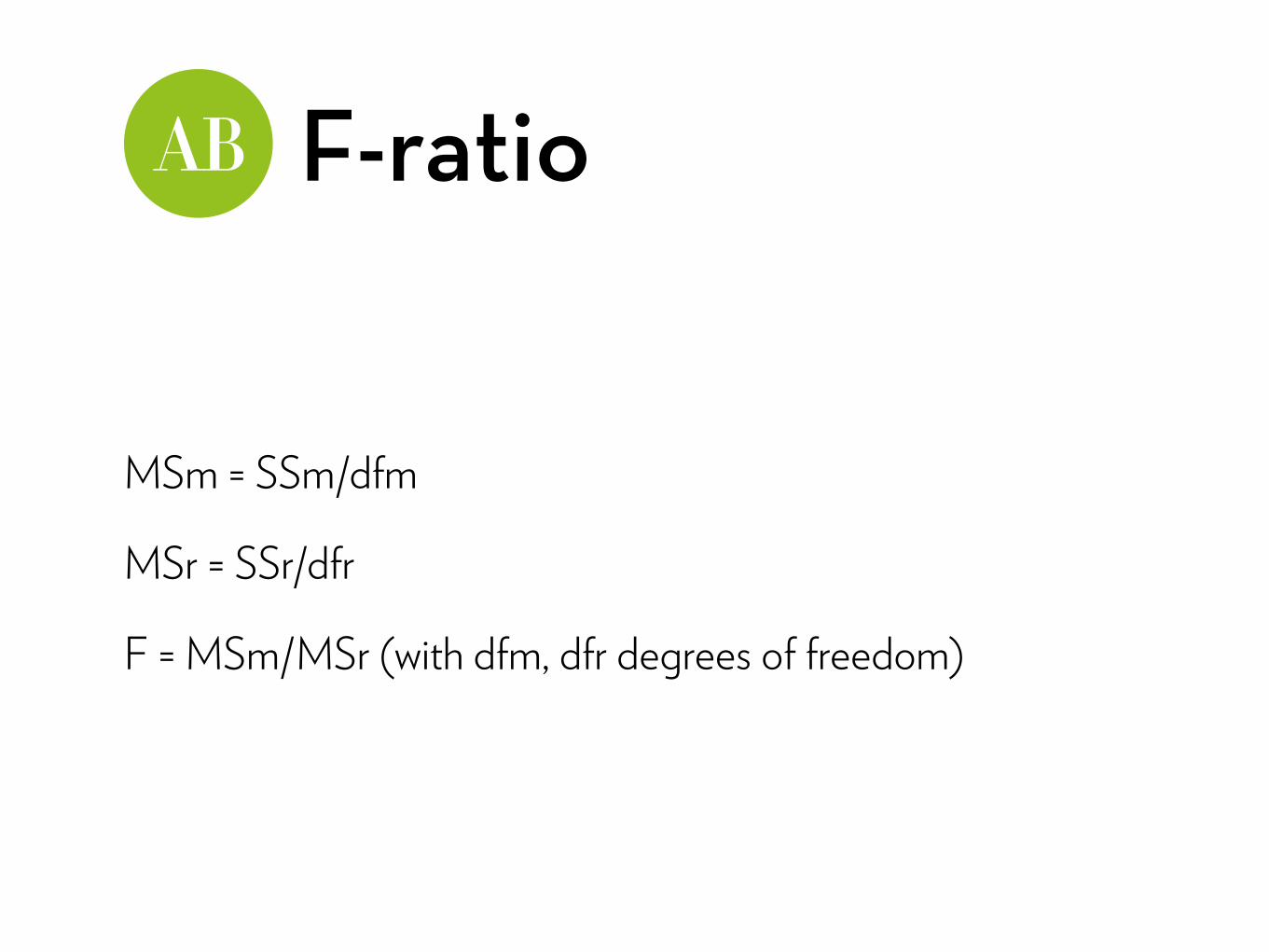
MSm = SSm/dfm

MSr = SSr/dfr

F = MSm/MSr (with dfm, dfr degrees of freedom)

Within-subjects in Rusing ezANOVA and lme

Within-subjects in RDataset “Bushtucker.dat” —> rename to “bush”

Effect of eating disgusting things on retching

Variables: participant: the participant ID stick_insect: time it takes before participant retches after eating a stick insect kangaroo_testicle: …after eating a kangaroo testicle fish eye: …after eating a fish eye witchetty grub: …after eating a witchetty grub (a larvae)

Reshape the data

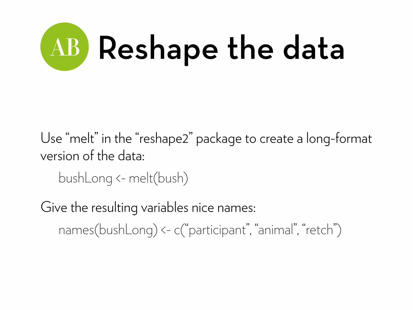
Use “melt” in the “reshape2” package to create a long-format version of the data:

bushLong <- melt(bush)

Give the resulting variables nice names: names(bushLong) <- c(“participant”, “animal”, “retch”)

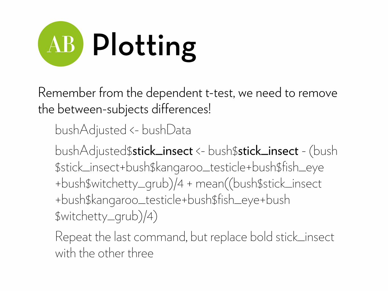
PlottingRemember from the dependent t-test, we need to remove the between-subjects differences!

bushAdjusted <- bushData bushAdjusted$stick_insect <- bush$stick_insect - (bush$stick_insect+bush$kangaroo_testicle+bush$fish_eye+bush$witchetty_grub)/4 + mean((bush$stick_insect+bush$kangaroo_testicle+bush$fish_eye+bush$witchetty_grub)/4) Repeat the last command, but replace bold stick_insect with the other three

Plotting

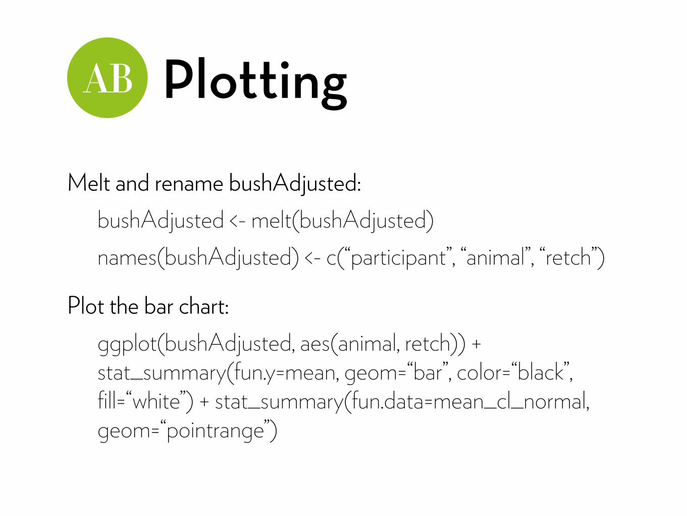
Melt and rename bushAdjusted: bushAdjusted <- melt(bushAdjusted) names(bushAdjusted) <- c(“participant”, “animal”, “retch”)

Plot the bar chart: ggplot(bushAdjusted, aes(animal, retch)) + stat_summary(fun.y=mean, geom=“bar”, color=“black”, fill=“white”) + stat_summary(fun.data=mean_cl_normal, geom=“pointrange”)

Plotting

Boxplots: ggplot(bushLong,aes(animal,retch)) + geom_boxplot()

ContrastsLevels of animal variable:

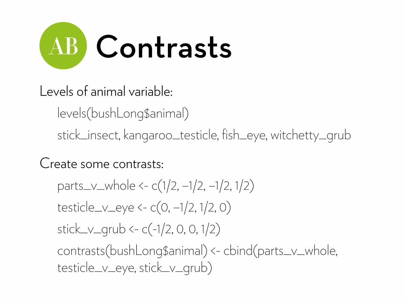
levels(bushLong$animal) stick_insect, kangaroo_testicle, fish_eye, witchetty_grub

Create some contrasts: parts_v_whole <- c(1/2, –1/2, –1/2, 1/2) testicle_v_eye <- c(0, –1/2, 1/2, 0) stick_v_grub <- c(-1/2, 0, 0, 1/2) contrasts(bushLong$animal) <- cbind(parts_v_whole, testicle_v_eye, stick_v_grub)

ezANOVA

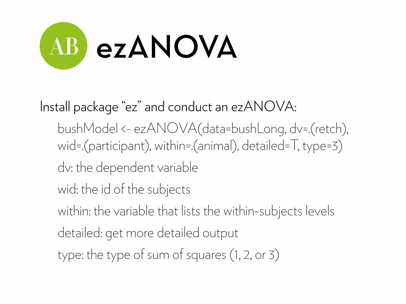
Install package “ez” and conduct an ezANOVA: bushModel <- ezANOVA(data=bushLong, dv=.(retch), wid=.(participant), within=.(animal), detailed=T, type=3) dv: the dependent variable wid: the id of the subjects within: the variable that lists the within-subjects levels detailed: get more detailed output type: the type of sum of squares (1, 2, or 3)

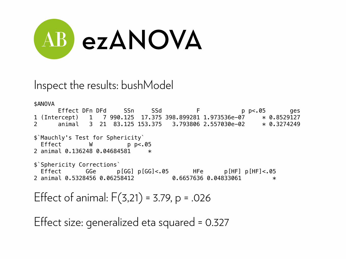
ezANOVAInspect the results: bushModel $ANOVA Effect DFn DFd SSn SSd F p p<.05 ges 1 (Intercept) 1 7 990.125 17.375 398.899281 1.973536e-07 * 0.8529127 2 animal 3 21 83.125 153.375 3.793806 2.557030e-02 * 0.3274249

$`Mauchly's Test for Sphericity` Effect W p p<.05 2 animal 0.136248 0.04684581 *

$`Sphericity Corrections` Effect GGe p[GG] p[GG]<.05 HFe p[HF] p[HF]<.05 2 animal 0.5328456 0.06258412 0.6657636 0.04833061 *

Effect of animal: F(3,21) = 3.79, p = .026

Effect size: generalized eta squared = 0.327

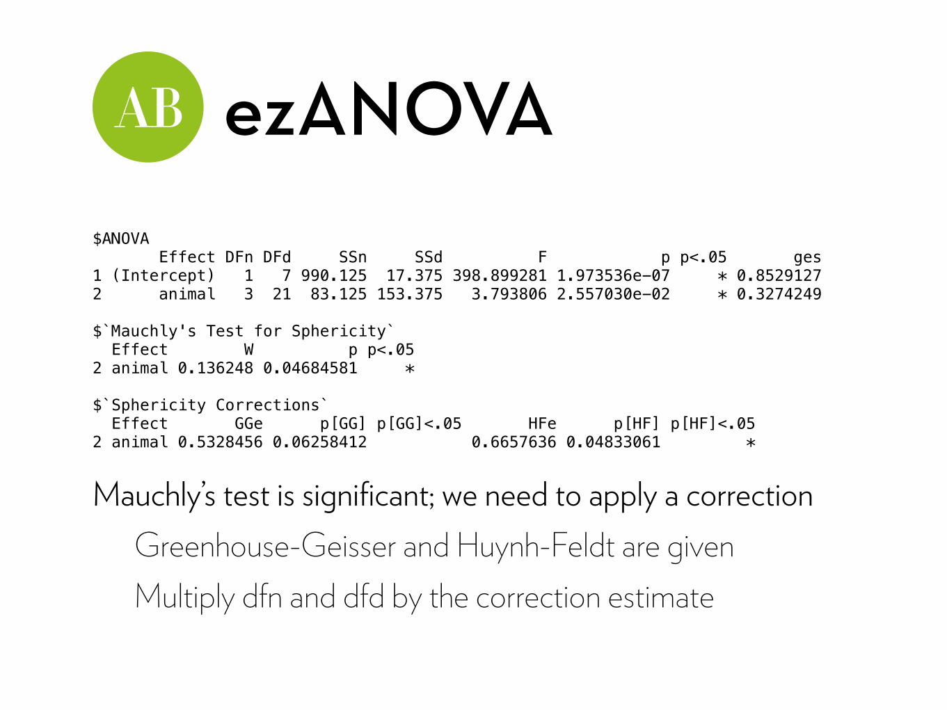
ezANOVA$ANOVA Effect DFn DFd SSn SSd F p p<.05 ges 1 (Intercept) 1 7 990.125 17.375 398.899281 1.973536e-07 * 0.8529127 2 animal 3 21 83.125 153.375 3.793806 2.557030e-02 * 0.3274249

$`Mauchly's Test for Sphericity` Effect W p p<.05 2 animal 0.136248 0.04684581 *

$`Sphericity Corrections` Effect GGe p[GG] p[GG]<.05 HFe p[HF] p[HF]<.05 2 animal 0.5328456 0.06258412 0.6657636 0.04833061 *

Mauchly’s test is significant; we need to apply a correction Greenhouse-Geisser and Huynh-Feldt are given Multiply dfn and dfd by the correction estimate

ezANOVA

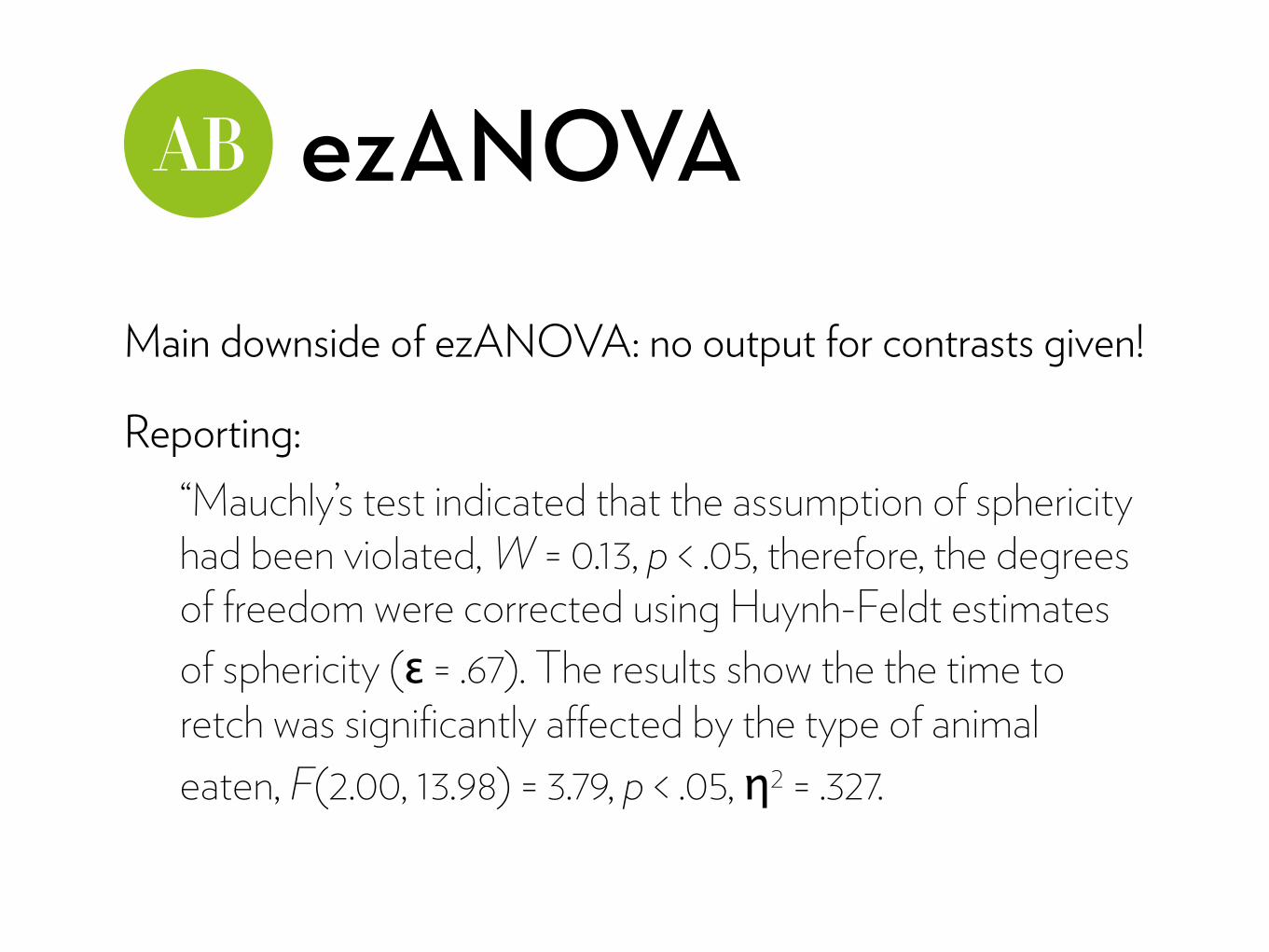
Main downside of ezANOVA: no output for contrasts given!

Reporting: “Mauchly’s test indicated that the assumption of sphericity had been violated, W = 0.13, p < .05, therefore, the degrees of freedom were corrected using Huynh-Feldt estimates of sphericity (ε = .67). The results show the the time to retch was significantly affected by the type of animal eaten, F(2.00, 13.98) = 3.79, p < .05, η2 = .327.

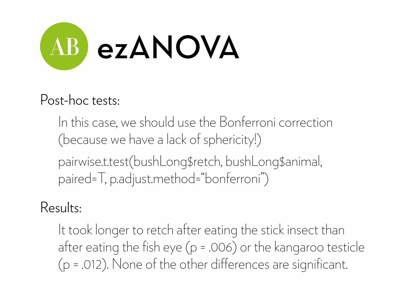
ezANOVAPost-hoc tests:

In this case, we should use the Bonferroni correction (because we have a lack of sphericity!) pairwise.t.test(bushLong$retch, bushLong$animal, paired=T, p.adjust.method=“bonferroni”)

Results: It took longer to retch after eating the stick insect than after eating the fish eye (p = .006) or the kangaroo testicle (p = .012). None of the other differences are significant.

lme

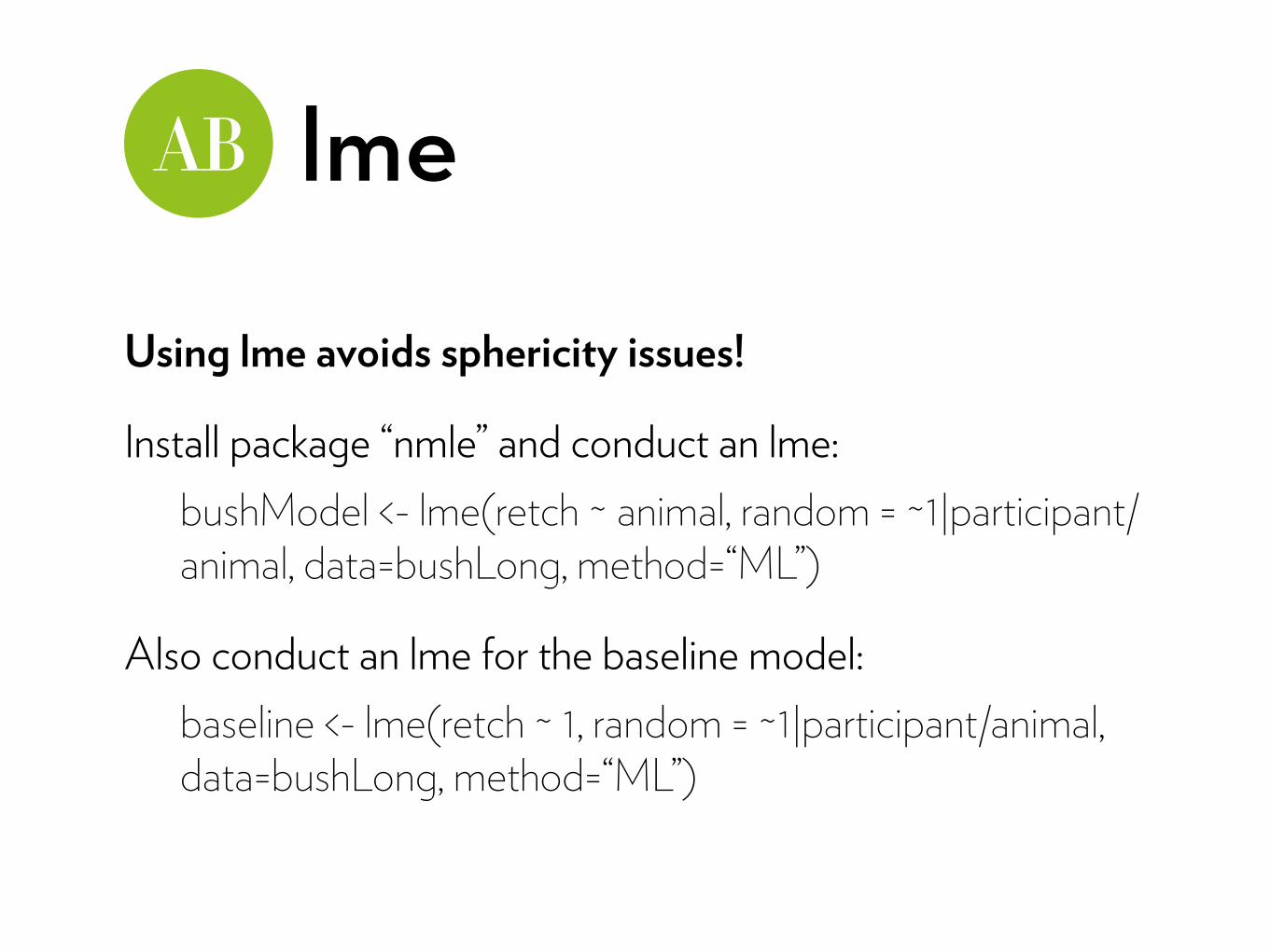
Using lme avoids sphericity issues!

Install package “nmle” and conduct an lme: bushModel <- lme(retch ~ animal, random = ~1|participant/animal, data=bushLong, method=“ML”)

Also conduct an lme for the baseline model: baseline <- lme(retch ~ 1, random = ~1|participant/animal, data=bushLong, method=“ML”)

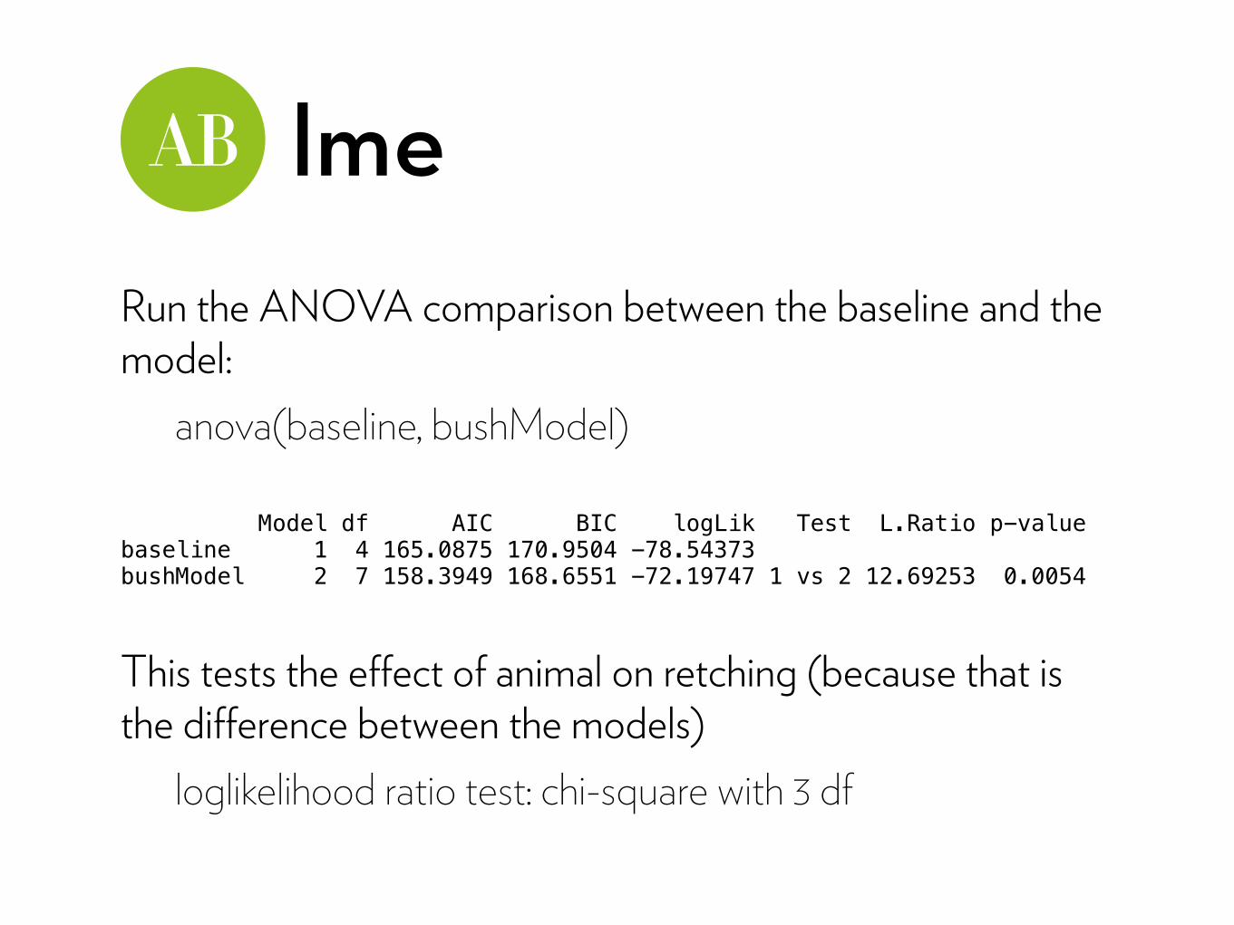
lmeRun the ANOVA comparison between the baseline and the model:

anova(baseline, bushModel)

Model df AIC BIC logLik Test L.Ratio p-value baseline 1 4 165.0875 170.9504 -78.54373 bushModel 2 7 158.3949 168.6551 -72.19747 1 vs 2 12.69253 0.0054

This tests the effect of animal on retching (because that is the difference between the models)

loglikelihood ratio test: chi-square with 3 df

lme

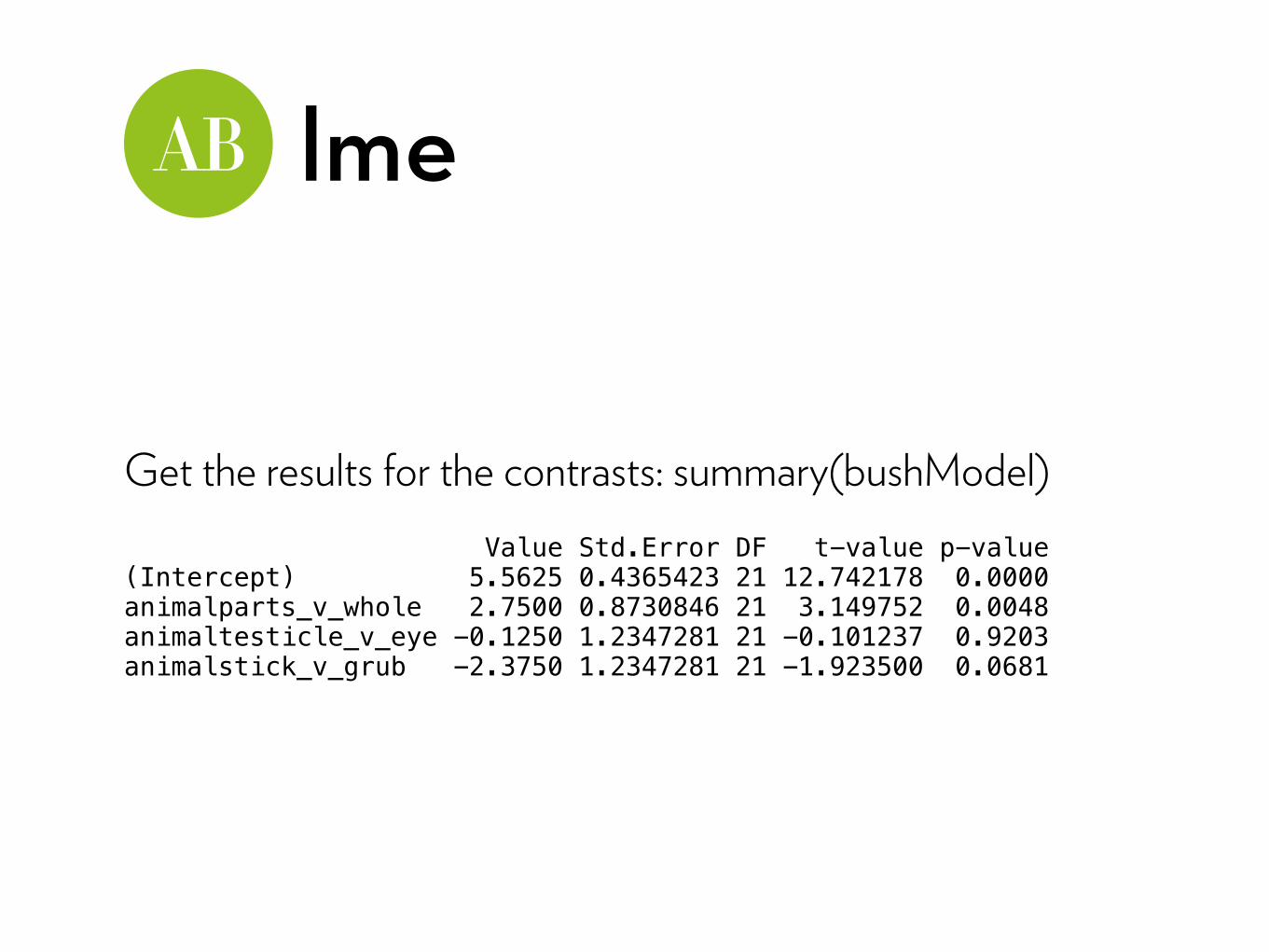
Get the results for the contrasts: summary(bushModel) Value Std.Error DF t-value p-value (Intercept) 5.5625 0.4365423 21 12.742178 0.0000 animalparts_v_whole 2.7500 0.8730846 21 3.149752 0.0048 animaltesticle_v_eye -0.1250 1.2347281 21 -0.101237 0.9203 animalstick_v_grub -2.3750 1.2347281 21 -1.923500 0.0681

lme

Reporting: The type of animal consumed had a significant effect on the time taken to retch, χ2(3) = 12.69, p = .005. Orthogonal contrasts revealed that retching times were significantly quicker for animal parts (testicle and eye) than for whole animals (stick insect and witchetty grub), b = 2.75, t(21) = 3.15, p = .005); there was no significant difference between testicles and eyes (b = –0.125, t(21) = –0.101, p = .920), or between grub than stick (b = –2.375, t(21) = –1.92, p = .068).

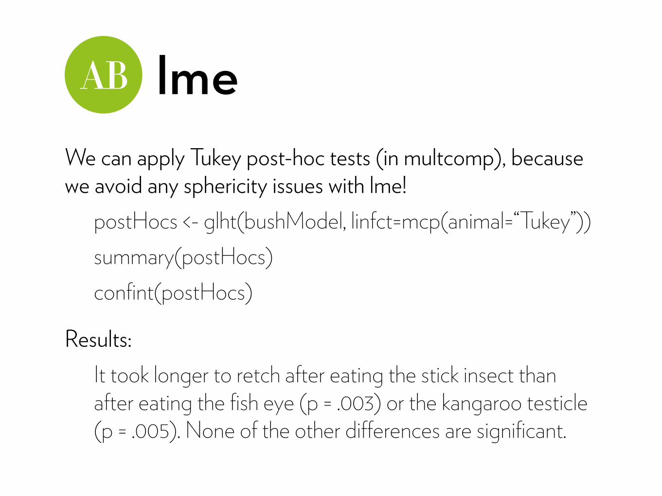
lmeWe can apply Tukey post-hoc tests (in multcomp), because we avoid any sphericity issues with lme!

postHocs <- glht(bushModel, linfct=mcp(animal=“Tukey”)) summary(postHocs) confint(postHocs)

Results: It took longer to retch after eating the stick insect than after eating the fish eye (p = .003) or the kangaroo testicle (p = .005). None of the other differences are significant.

Robust methods

WRS2 package functions work on the wide versions of the dataset (bushData)

First, though, we need to keep only the used columns: bushData2 <- bushData[,c("stick_insect", "kangaroo_testicle", "fish_eye", "witchetty_grub")]

Robust methods

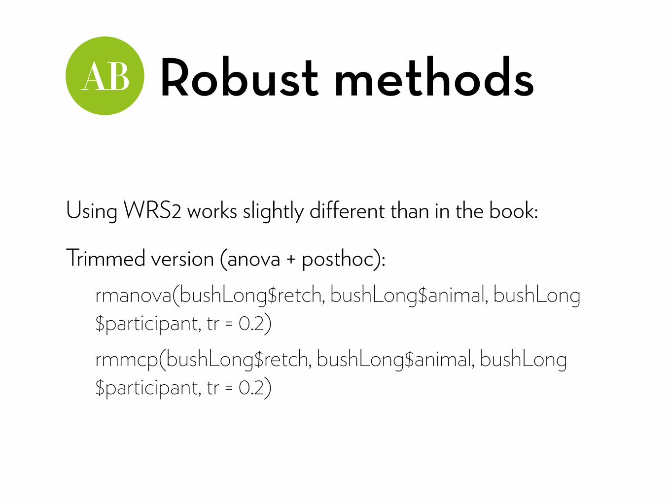
Using WRS2 works slightly different than in the book:

Trimmed version (anova + posthoc): rmanova(bushLong$retch, bushLong$animal, bushLong$participant, tr = 0.2) rmmcp(bushLong$retch, bushLong$animal, bushLong$participant, tr = 0.2)

Robust methods

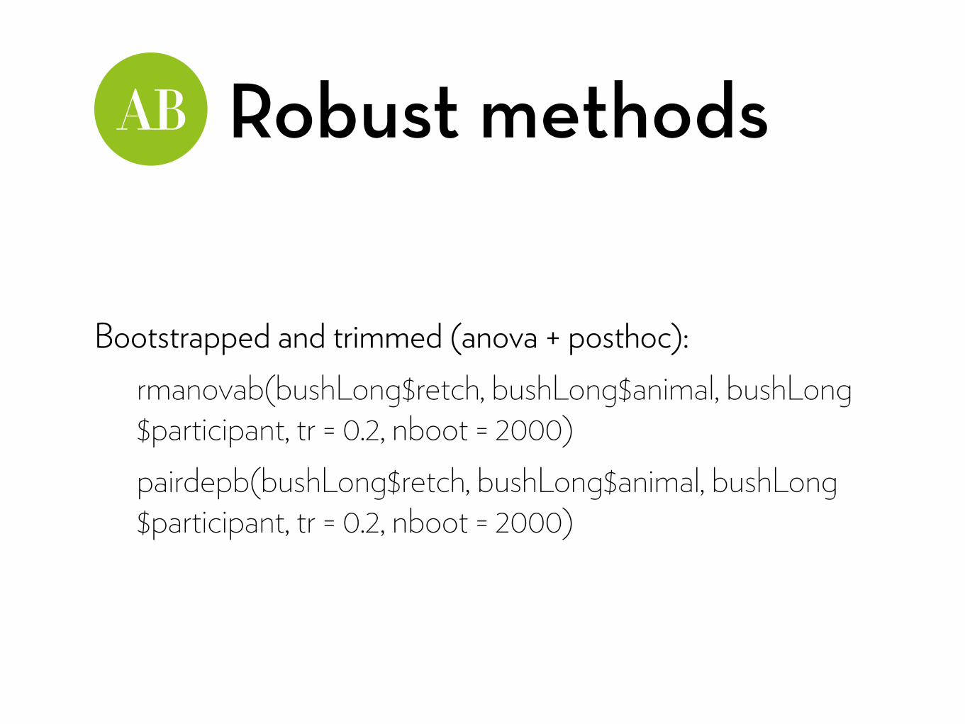
Bootstrapped and trimmed (anova + posthoc): rmanovab(bushLong$retch, bushLong$animal, bushLong$participant, tr = 0.2, nboot = 2000) pairdepb(bushLong$retch, bushLong$animal, bushLong$participant, tr = 0.2, nboot = 2000)

Factorial repeated in Rusing ezANOVA and lme

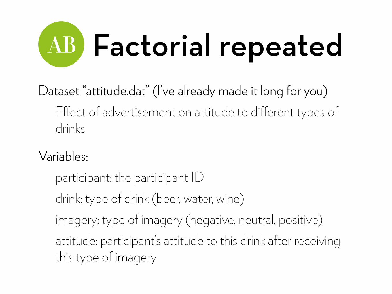
Factorial repeatedDataset “attitude.dat” (I’ve already made it long for you)

Effect of advertisement on attitude to different types of drinks

Variables: participant: the participant ID drink: type of drink (beer, water, wine) imagery: type of imagery (negative, neutral, positive) attitude: participant’s attitude to this drink after receiving this type of imagery

Plotting

Create boxplots: ggplot(attitude,aes(drink,attitude))+geom_boxplot()+facet_wrap(~imagery)

Contrasts

For drink, test alcohol vs water, and beer vs wine: alcohol_v_water <- c(1/3, -2/3, 1/3) beer_v_wine <-c(1/2, 0, -1/2) contrasts(attitude$drink) <- cbind(alcohol_v_water, beer_v_wine)

Contrasts

For imagery, test negative vs other, and positive vs neutral: neg_v_other <- c(-2/3, 1/3, 1/3) pos_v_neutral <-c(0, -1/2, 1/2) contrasts(attitude$imagery) <- cbind(neg_v_other, pos_v_neutral)

ezANOVA

Conduct an ezANOVA: a1 <- ezANOVA(data=attitude, dv=.(attitude), wid=.(participant), within=.(imagery, drink), detailed=T, type=3)

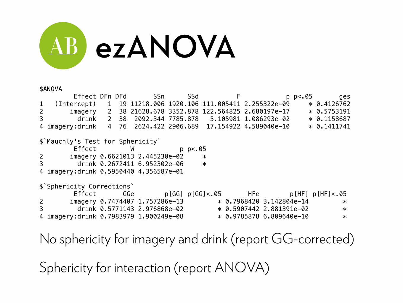
ezANOVA$ANOVA Effect DFn DFd SSn SSd F p p<.05 ges 1 (Intercept) 1 19 11218.006 1920.106 111.005411 2.255322e-09 * 0.4126762 2 imagery 2 38 21628.678 3352.878 122.564825 2.680197e-17 * 0.5753191 3 drink 2 38 2092.344 7785.878 5.105981 1.086293e-02 * 0.1158687 4 imagery:drink 4 76 2624.422 2906.689 17.154922 4.589040e-10 * 0.1411741

$`Mauchly's Test for Sphericity` Effect W p p<.05 2 imagery 0.6621013 2.445230e-02 * 3 drink 0.2672411 6.952302e-06 * 4 imagery:drink 0.5950440 4.356587e-01

$`Sphericity Corrections` Effect GGe p[GG] p[GG]<.05 HFe p[HF] p[HF]<.05 2 imagery 0.7474407 1.757286e-13 * 0.7968420 3.142804e-14 * 3 drink 0.5771143 2.976868e-02 * 0.5907442 2.881391e-02 * 4 imagery:drink 0.7983979 1.900249e-08 * 0.9785878 6.809640e-10 *

No sphericity for imagery and drink (report GG-corrected)

Sphericity for interaction (report ANOVA)

−10

0

10

20

30

beer water winedrink

attitude

imagery

neg

neutral

pos

ezANOVA

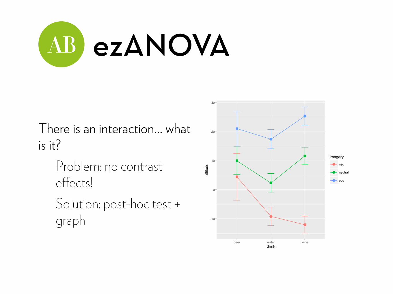
There is an interaction… what is it?

Problem: no contrast effects! Solution: post-hoc test + graph

ezANOVA

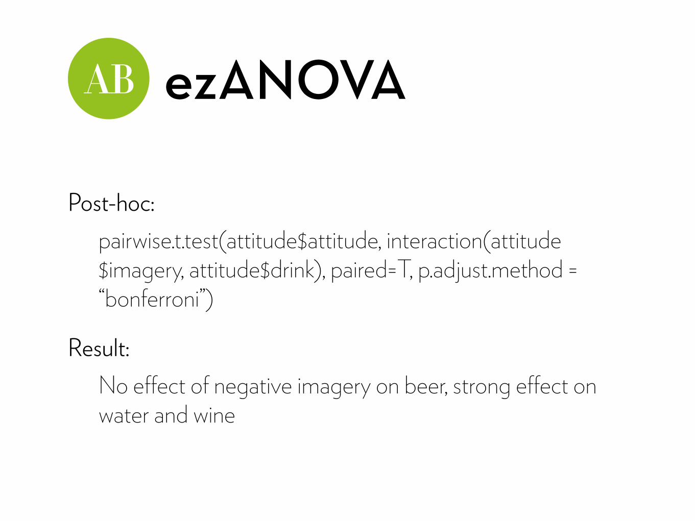
Post-hoc: pairwise.t.test(attitude$attitude, interaction(attitude$imagery, attitude$drink), paired=T, p.adjust.method = “bonferroni”)

Result: No effect of negative imagery on beer, strong effect on water and wine

ezANOVAReporting:

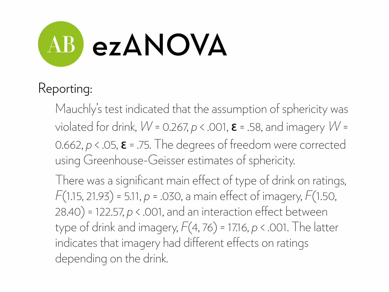
Mauchly’s test indicated that the assumption of sphericity was violated for drink, W = 0.267, p < .001, ε = .58, and imagery W = 0.662, p < .05, ε = .75. The degrees of freedom were corrected using Greenhouse-Geisser estimates of sphericity. There was a significant main effect of type of drink on ratings, F(1.15, 21.93) = 5.11, p = .030, a main effect of imagery, F(1.50, 28.40) = 122.57, p < .001, and an interaction effect between type of drink and imagery, F(4, 76) = 17.16, p < .001. The latter indicates that imagery had different effects on ratings depending on the drink.

ezANOVA

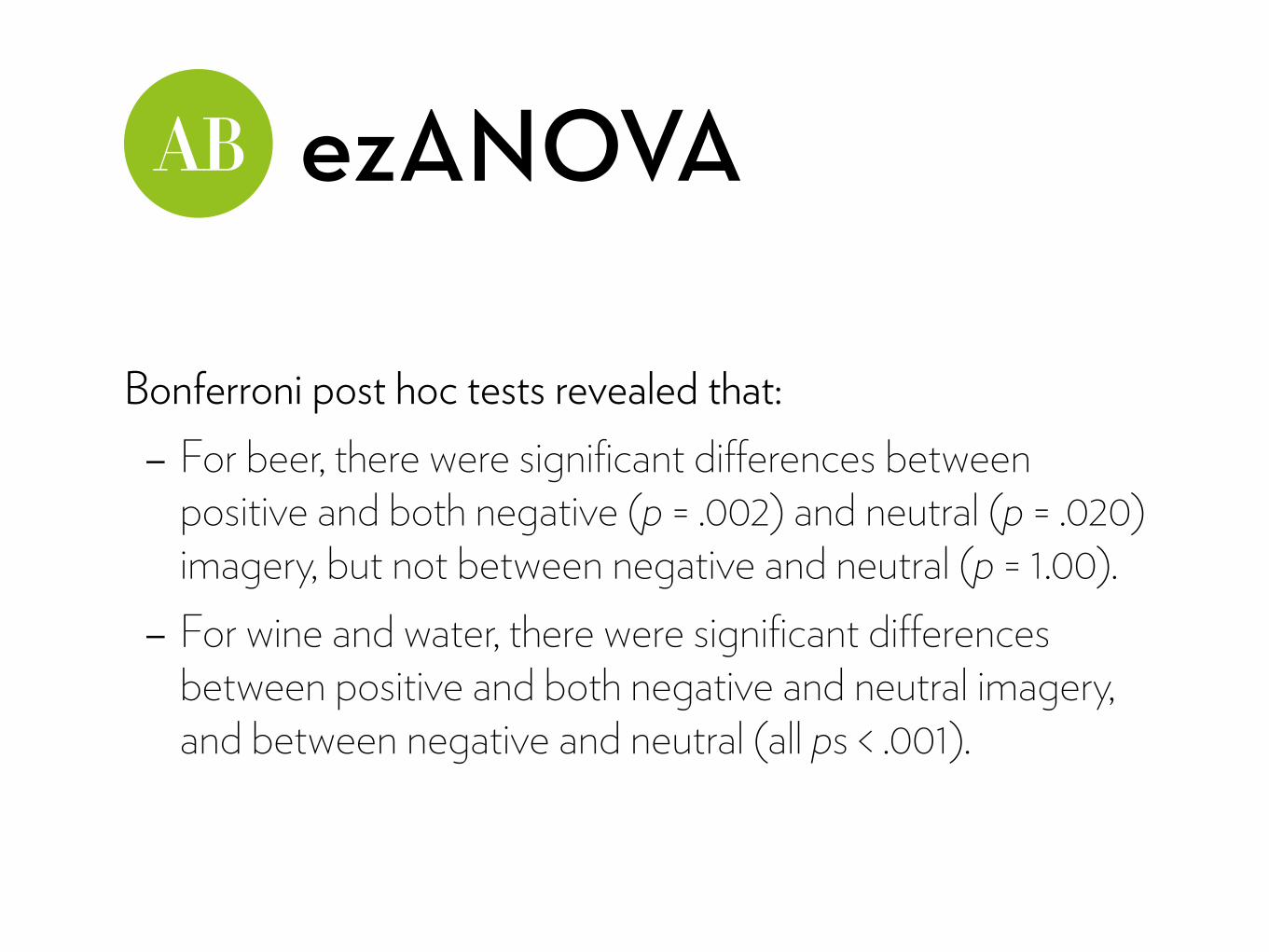
Bonferroni post hoc tests revealed that:

- For beer, there were significant differences between positive and both negative (p = .002) and neutral (p = .020) imagery, but not between negative and neutral (p = 1.00).

- For wine and water, there were significant differences between positive and both negative and neutral imagery, and between negative and neutral (all ps < .001).

lme

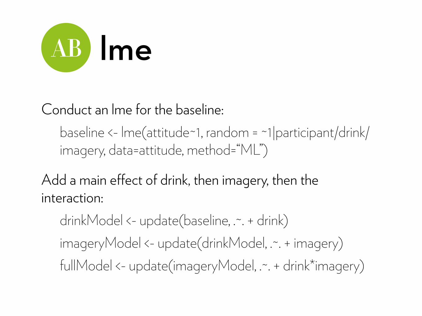
Conduct an lme for the baseline: baseline <- lme(attitude~1, random = ~1|participant/drink/imagery, data=attitude, method=“ML”)

Add a main effect of drink, then imagery, then the interaction:

drinkModel <- update(baseline, .~. + drink) imageryModel <- update(drinkModel, .~. + imagery) fullModel <- update(imageryModel, .~. + drink*imagery)

lme

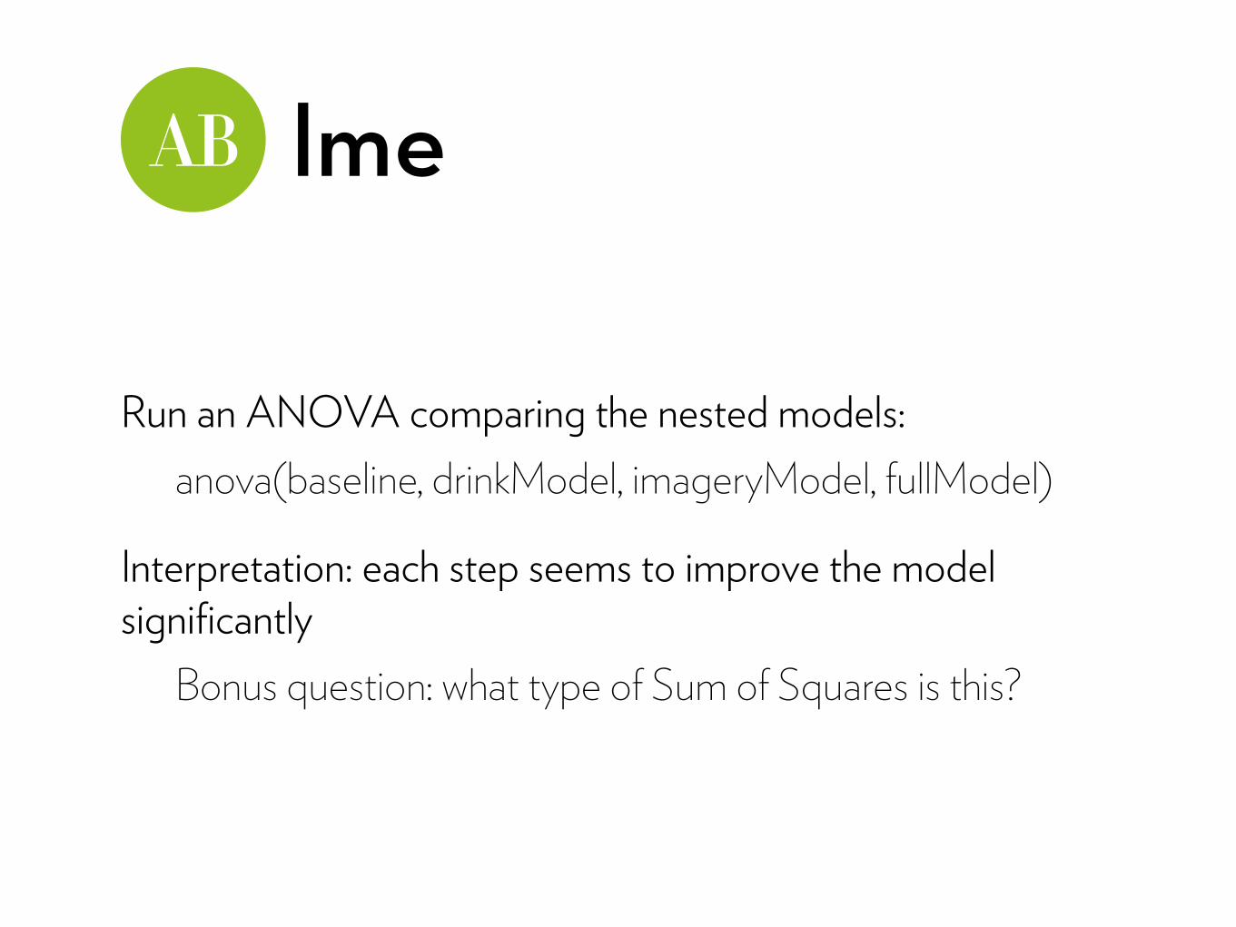
Run an ANOVA comparing the nested models: anova(baseline, drinkModel, imageryModel, fullModel)

Interpretation: each step seems to improve the model significantly

Bonus question: what type of Sum of Squares is this?

lme

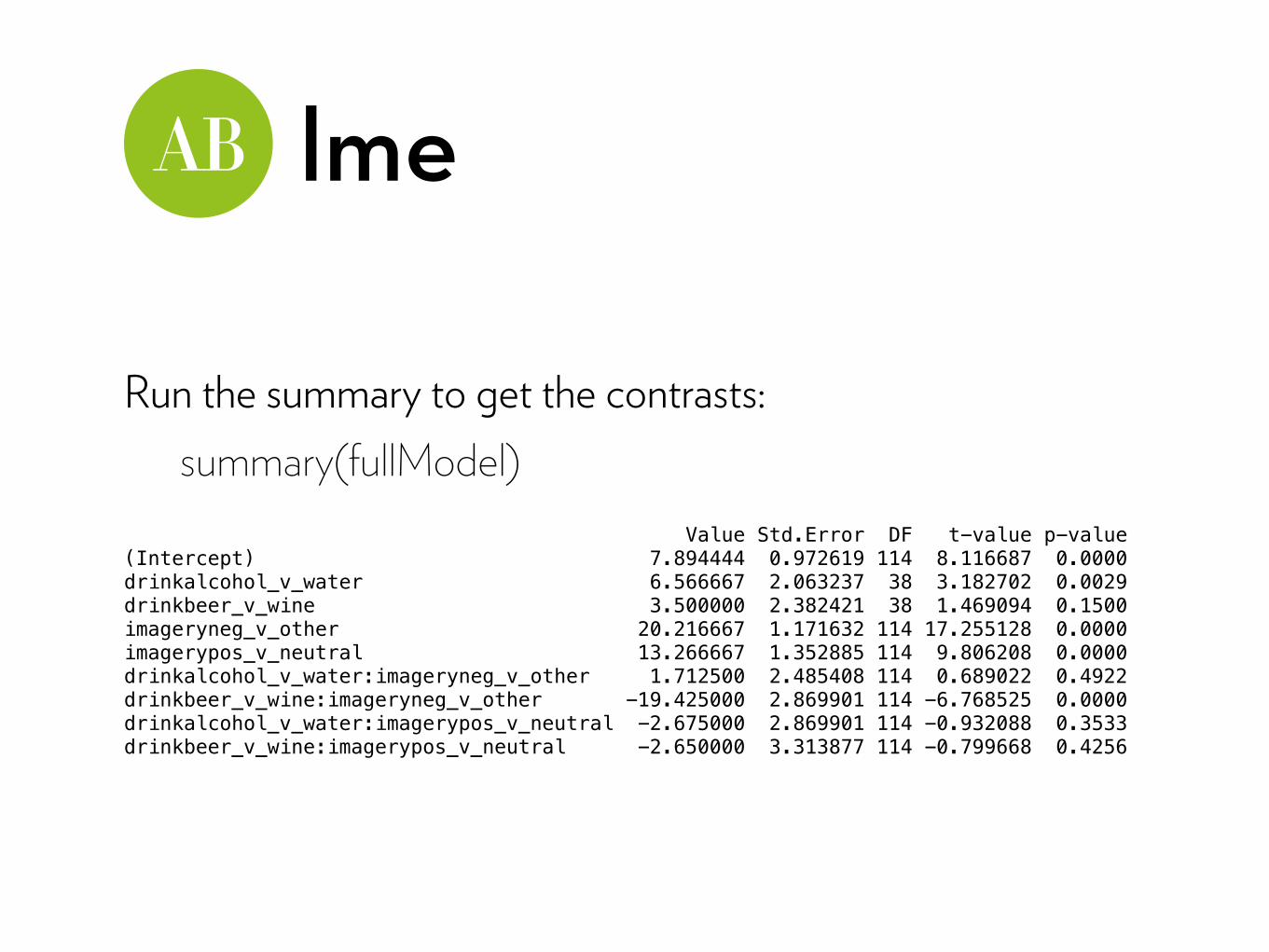
Run the summary to get the contrasts: summary(fullModel)

Value Std.Error DF t-value p-value (Intercept) 7.894444 0.972619 114 8.116687 0.0000 drinkalcohol_v_water 6.566667 2.063237 38 3.182702 0.0029 drinkbeer_v_wine 3.500000 2.382421 38 1.469094 0.1500 imageryneg_v_other 20.216667 1.171632 114 17.255128 0.0000 imagerypos_v_neutral 13.266667 1.352885 114 9.806208 0.0000 drinkalcohol_v_water:imageryneg_v_other 1.712500 2.485408 114 0.689022 0.4922 drinkbeer_v_wine:imageryneg_v_other -19.425000 2.869901 114 -6.768525 0.0000 drinkalcohol_v_water:imagerypos_v_neutral -2.675000 2.869901 114 -0.932088 0.3533 drinkbeer_v_wine:imagerypos_v_neutral -2.650000 3.313877 114 -0.799668 0.4256

lme

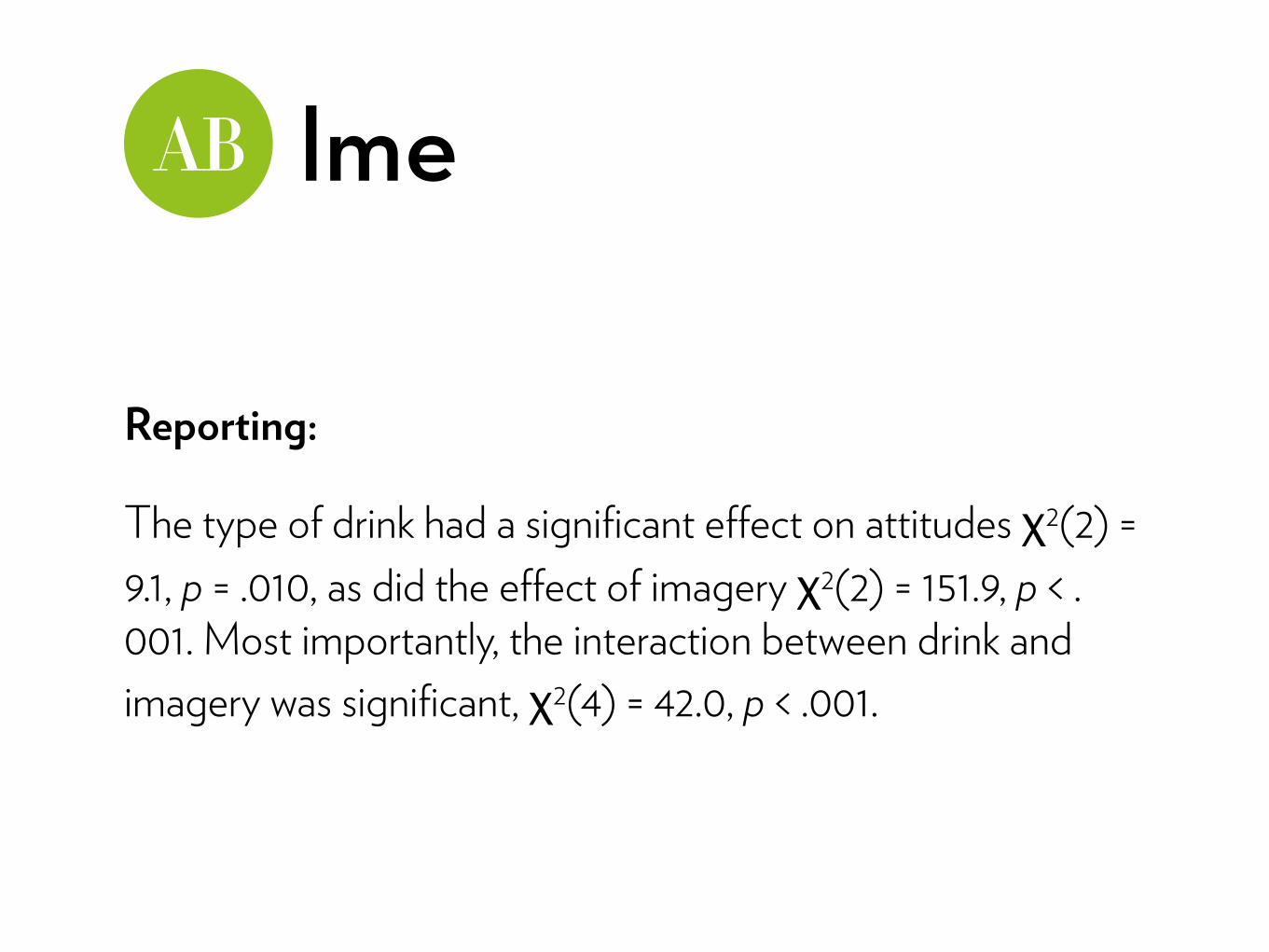
Reporting:

The type of drink had a significant effect on attitudes χ2(2) = 9.1, p = .010, as did the effect of imagery χ2(2) = 151.9, p < .001. Most importantly, the interaction between drink and imagery was significant, χ2(4) = 42.0, p < .001.

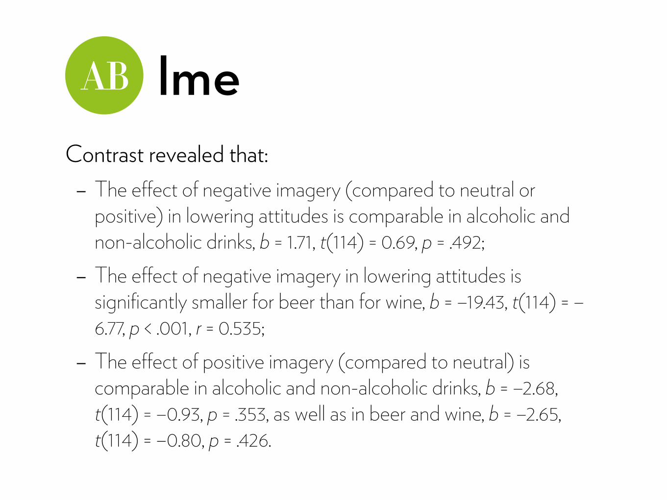
lmeContrast revealed that: - The effect of negative imagery (compared to neutral or

positive) in lowering attitudes is comparable in alcoholic and non-alcoholic drinks, b = 1.71, t(114) = 0.69, p = .492;

- The effect of negative imagery in lowering attitudes is significantly smaller for beer than for wine, b = –19.43, t(114) = –6.77, p < .001, r = 0.535;

- The effect of positive imagery (compared to neutral) is comparable in alcoholic and non-alcoholic drinks, b = –2.68, t(114) = –0.93, p = .353, as well as in beer and wine, b = –2.65, t(114) = –0.80, p = .426.

“It is the mark of a truly intelligent person to be moved by statistics.”

George Bernard Shaw