Linear predictors for nonlinear dynamicalsystems: Koopman operator meets model

predictive control

Milan Korda1, Igor Mezic1

Draft of January 31, 2018

Abstract

This paper presents a class of linear predictors for nonlinear controlled dynamicalsystems. The basic idea is to lift (or embed) the nonlinear dynamics into a higherdimensional space where its evolution is approximately linear. In an uncontrolled set-ting, this procedure amounts to numerical approximations of the Koopman operatorassociated to the nonlinear dynamics. In this work, we extend the Koopman operatorto controlled dynamical systems and apply the Extended Dynamic Mode Decomposi-tion (EDMD) to compute a finite-dimensional approximation of the operator in such away that this approximation has the form of a linear controlled dynamical system. Innumerical examples, the linear predictors obtained in this way exhibit a performancesuperior to existing linear predictors such as those based on local linearization or theso called Carleman linearization. Importantly, the procedure to construct these linearpredictors is completely data-driven and extremely simple – it boils down to a nonlin-ear transformation of the data (the lifting) and a linear least squares problem in thelifted space that can be readily solved for large data sets. These linear predictors canbe readily used to design controllers for the nonlinear dynamical system using linearcontroller design methodologies. We focus in particular on model predictive control(MPC) and show that MPC controllers designed in this way enjoy computational com-plexity of the underlying optimization problem comparable to that of MPC for a lineardynamical system with the same number of control inputs and the same dimensionof the state-space. Importantly, linear inequality constraints on the state and controlinputs as well as nonlinear constraints on the state can be imposed in a linear fashionin the proposed MPC scheme. Similarly, cost functions nonlinear in the state variablecan be handled in a linear fashion. We treat both the full-state measurement caseand the input-output case, as well as systems with disturbances / noise. Numericalexamples demonstrate the approach.

Keywords: Koopman operator, Model predictive control, Data-driven control design, Optimalcontrol, Lifting, Embedding.

1Milan Korda and Igor Mezic are with the University of California, Santa Barbara,milan.korda@engineering.ucsb.edu, mezic@engineering.ucsb.edu

1

1 Introduction

This paper presents a class of linear predictors for nonlinear controlled dynamical systems.By a predictor, we mean an artificial dynamical system that can predict the future state (oroutput) of a given nonlinear dynamical system based on the measurement of the current state(or output) and current and future inputs of the system. We focus on predictors possessinga linear structure that allows established linear control design methodologies to be used todesign controllers for nonlinear dynamical systems.

The key step in obtaining accurate predictions of a nonlinear dynamical system as theoutput of a linear dynamical system is lifting of the state-space to a higher dimensional space,where the evolution of this lifted state is (approximately) linear. For uncontrolled dynamicalsystems, this idea can be rigorously justified using the Koopman operator theory [15]. TheKoopman operator is a linear operator that governs the evolution of scalar functions (oftenreferred to as observables) along trajectories of a given nonlinear dynamical system. A finite-dimensional approximation of this operator, acting on a given finite-dimensional subspace ofall functions, can be viewed as a predictor of the evolution of the values of these functionsalong the trajectories of the nonlinear dynamical system and hence also as a predictor of thevalues of the state variables themselves provided that they lie in the subspace of functionsthe operator is truncated on. In the uncontrolled context, this idea goes back to the seminalworks of Koopman, Carleman and Von Neumann [9, 4, 10].

In this work, we extend the definition of the Koopman operator to controlled dynamicalsystems by viewing the controlled dynamical system as an uncontrolled one evolving onan extended state-space given by the product of the original state-space and the space ofall control sequences. Subsequently, we use a modified version of the Extended DynamicMode Decomposition (EDMD) [24] to compute a finite-dimensional approximation of thiscontrolled Koopman operator. In particular we impose a specific structure on the set ofobservables appearing in the EDMD such that the resulting approximation of the operatorhas the form of a linear controlled dynamical system. Importantly, the procedure to constructthese linear predictors is completely data-driven (i.e., does not require the knowledge of theunderlying dynamics) and extremely simple – it boils down to a nonlinear transformationof the data (the lifting) and a linear least squares problem in the lifted space that canreadily solved for large data sets using linear algebra. On the numerical examples tested,the linear predictors obtained in this way exhibit a predictive performance superior comparedto both Carleman linearization as well as local linearization methods. For a related work onextending Koopman operator methods to controlled dynamical systems, see [2, 17, 18, 23].See also [21, 20] and [13] for the use of Koopman operator methods for state estimation andnonlinear system identification, respectively.

Finally, we demonstrate in detail the use of these predictors for model predictive control(MPC) design; see the survey [14] or the book [7] for an overview of MPC. In particular weshow that these predictors can be used to design MPC controllers for nonlinear dynamicalsystems with computational complexity comparable to MPC controllers for linear dynami-cal systems with the same number of control inputs and states. Indeed, the resulting MPCscheme is extremely simple: In each time step of closed-loop operation it involves one eval-uation of a family of nonlinear functions (the lifting) to obtain the initial condition of the

2

linear predictor and the solution of a convex quadratic program affinely parametrized by thislifted initial condition. Importantly, nonlinear cost functions and constraints can be handledin a linear fashion by including all nonlinear terms appearing in these functions among thelifting functions. Therefore, the proposed scheme can be readily used for predictive controlof nonlinear dynamical systems, using the tailored and extremely efficient solvers for linearMPC (in our case qpOASES [6]), thereby avoiding the troublesome and computationallyexpensive solution of nonconvex optimization problems encountered in classical nonlinearMPC schemes [7].

The paper is organized as follows: In Section 2 we describe the problem setup and the basicidea behind the use of linear predictors for nonlinear dynamical systems. In Section 3 wederive these linear predictors as finite-dimensional approximations to the Koopman operatorextended to nonlinear dynamical systems. In Section 4 we describe a numerical algorithmfor obtaining these linear predictors. In Section 5 we describe the use of these predictors formodel predictive control. In Section 7 we discuss extensions of the approach to input outputsystems (Section 7.1) and to systems with disturbances / noise (Section 7.2). In Section 8we present numerical examples.

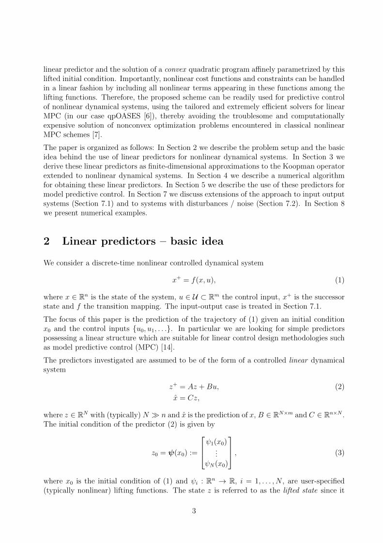
2 Linear predictors – basic idea

We consider a discrete-time nonlinear controlled dynamical system

x+ = f(x, u), (1)

where x ∈ Rn is the state of the system, u ∈ U ⊂ Rm the control input, x+ is the successorstate and f the transition mapping. The input-output case is treated in Section 7.1.

The focus of this paper is the prediction of the trajectory of (1) given an initial conditionx0 and the control inputs {u0, u1, . . .}. In particular we are looking for simple predictorspossessing a linear structure which are suitable for linear control design methodologies suchas model predictive control (MPC) [14].

The predictors investigated are assumed to be of the form of a controlled linear dynamicalsystem

z+ = Az +Bu, (2)

x = Cz,

where z ∈ RN with (typically) N � n and x is the prediction of x, B ∈ RN×m and C ∈ Rn×N .The initial condition of the predictor (2) is given by

z0 = ψ(x0) :=

ψ1(x0)...

ψN(x0)

, (3)

where x0 is the initial condition of (1) and ψi : Rn → R, i = 1, . . . , N , are user-specified(typically nonlinear) lifting functions. The state z is referred to as the lifted state since it

3

evolves on a higher-dimensional, lifted, space1. Importantly, the control input u ∈ U of (2)remains unlifted and hence linear constraints on the control inputs can be imposed in a linearfashion. Notice also that the predicted state x is a linear function of the lifted state z andhence also linear constraints on the state can be readily imposed. Figure (1) depicts thisidea.

x+ = f(x, u)

z+ = Az + Bu

z0 = ψ(x0)

x0 given

x = Cz

Nonlinear system Linear predictor

�

dim(z) � dim(x)

H�

LQR

Linear control design

MPC

Figure 1: Linear predictor for a nonlinear controlled dynamical system – z is the lifted state evolving on ahigher-dimensional state space, x is the prediction of the true state x and ψ is a nonlinear lifting mapping.This predictor can then be used for control design using linear methods, in our case linear MPC.

Predictors of this form lend themselves immediately to linear feedback control design method-ologies. Importantly, however, the resulting feedback controller will be nonlinear in the orig-inal state x even though it may be (but is not required to be) linear in the lifted state z.Indeed, from any feedback controller κlift : RN → Rm for (2), we obtain a feedback controllerκ : Rn → Rm for the original system (1) defined by

κ(x) := κlift(ψ(x)). (4)

The idea is that if the true trajectory of x generated by (1) and the predicted trajectory ofx generated by (2) are close for each admissible input sequence, then the optimal controllerfor (2) should be close to the optimal controller for (1). In Section 3 we will see how thelinear predictors (2) can be derived within the Koopman operator framework extended tocontrolled dynamical systems.

Note, however, that in general one cannot hope that a trajectory of a linear system (2)will be an accurate prediction of the trajectory of a nonlinear system for all future times.Nevertheless, if the predictions are accurate on a long enough time interval, these predictorscan facilitate the use of linear control systems design methodologies. Especially suited forthis purpose is model predictive control (MPC) that uses only finite-time predictions togenerate the control input.

We will briefly mention in Section 3.2.2 how more complex, bi-linear, predictors of the form

z+ = Az + (Bz)u, (5)

x = Cz

1In general, the term “lifted state” may be misleading as, in principle, the same approach can be appliedto dynamical systems with states evolving on a (possibly infinite-dimensional) space M, with finitely manyobservations (or outputs) h(x) = [h1(x), . . . , hp(x)]> available at each time instance; the lifting is thenapplied to these output measurements (and possibly their time-delayed versions), i.e., ψi(x) in (19) becomesψi(h(x)) for some functions ψi : Rp → R. In other words, rather than the state itself we lift the output ofthe dynamical system. For a detailed treatment of the input-output case, see Section 7.1.

4

can be obtained within the same framework and argue that predictors of this form can beasymptotically tight (in a well defined sense). Nevertheless, predictors of the from (5) arenot immediately suited for linear control design and hence in this paper we focus on thelinear predictors (2).

3 Koopman operator – rationale behind the approach

We start by recalling the Koopman operator approach for the analysis of an uncontrolleddynamical system

x+ = f(x). (6)

The Koopman operator K : F → F is defined by

(Kψ)(x) = ψ(f(x)) (7)

for every ψ : Rn → R belonging to F , which is a space of functions (often referred to asobservables) invariant under the action of the Koopman operator. Importantly, the Koop-man operator is linear (but typically infinite-dimensional) even if the underlying dynamicalsystem is nonlinear. Crucially, this operator fully captures all properties of the underlyingdynamical system provided that the space of observables F contains the components of thestate xi, i.e, the mappings x 7→ xi belong to F for all i ∈ {1, . . . , n}. For a detailed surveyon Koopman operator and its applications, see [3].

3.1 Koopman operator for controlled systems

There are several ways of generalizing the Koopman operator to controlled systems; see,e.g., [18, 23]. In this paper we present a generalization that is both rigorous and practical.We define the Koopman operator associated to the controlled dynamical system (1) as theKoopman operator associated to the uncontrolled dynamical system evolving on the extendedstate-space defined as the product of the original state-space and the space of all controlsequences, i.e., in our case Rn × `(U), where `(U) is the space of all sequences (ui)

∞i=0 with

ui ∈ U . Elements of `(U) will be denoted by u := (ui)∞i=0. The dynamics of the extended

state

χ =

[xu

],

is described by

χ+ = F (χ) :=

[f(x,u(0))Su

], (8)

where S is the left shift operator, i.e. (Su)(i) = u(i + 1), and u(i) denotes the ith elementof the sequence u.

The Koopman operator K : H → H associated to (8) is defined by

(Kφ)(χ) = φ(F (χ)) (9)

for each φ : Rn × `(U)→ R belonging to some space of observables H.

5

The Koopman operator (9) is a linear operator fully describing the non-linear dynamicalsystem (1) provided that H contains the components of the non-extended state2 xi, i =1, . . . , n. For example, spectral properties of the operator K should provide information onspectral properties of the nonlinear dynamical system (1).

3.2 EDMD for controlled systems

In this paper, however, we are not interested in spectral properties but rather in time-domain prediction of trajectories of (1). To this end, we construct a finite-dimensionalapproximation to the operator K which will yield a predictor of the form (2). In order to doso, we adapt the extended dynamic mode decomposition algorithm (EDMD) of [24] to thecontrolled setting. The EDMD is a data-driven algorithm to construct finite-dimensionalapproximations to the Koopman operator. The algorithm assumes that a collection of data(χj, χ

+j ), j = 1, . . . , K satisfying χ+

j = F (χj) is available and seeks a matrix A (the transposeof the finite-dimensional approximation of K) minimizing

K∑j=1

‖φ(χ+j )−Aφ(χj)‖2

2, (10)

whereφ(χ) =

[φ1(χ) . . . φNφ(χ)

]>is a vector of lifting functions (or observables) φi : Rn × `(U) → R, i ∈ {1, . . . , Nφ}. Notethat χ = (x,u) is in general an infinite-dimensional object and hence the objective (10)cannot be evaluated in a finite time unless φi’s are chosen in a special way.

3.2.1 Linear predictors

In order to obtain a linear predictor (2) and a computable objective function in (10) weimpose that the functions φi are of the form

φi(x,u) = ψi(x) + Li(u), (11)

where ψi : Rn → R is in general nonlinear but Li : `(U) → R is linear. Without loss ofgenerality (by linearity and causality) we can assume that Nφ = N +m for some N > 0 andthat the vector of lifting functions φ = [φ1, . . . , φNφ ]> is of the form

φ(x,u) =

[ψ(x)u(0)

], (12)

where ψ = [ψ1, . . . ψN ]> and u(0) ∈ Rm denotes the first component of the sequence u. Sincewe are not interested in predicting future values of the control sequence, we can disregardthe last m components of each term φ(χ+

j )−Aφ(χj) in (10). Denoting A the first N rows

2Note that the definition of the Koopman operator implicitly assumes that H is invariant under the actionof K and hence in the controlled setting H necessarily contains functions depending on u.

6

of A and decomposing this matrix such that A = [A,B] with A ∈ RN×N , B ∈ RN×m andusing the notation χj = (xj,uj) in (10), leads to the minimization problem

minA,B

K∑j=1

‖ψ(x+j )− Aψ(xj)−Buj(0)‖2

2. (13)

Minimizing (13) over A and B leads to the predictor of the form (2) starting from the initialcondition

z0 = ψ(x0) :=

ψ1(x0)...

ψN(x0)

. (14)

The matrix C is obtained simply as the best projection of x onto the span of ψi’s in a leastsquares sense, i.e., as the solution to

minC

K∑j=1

‖xj − Cψ(xj)‖22. (15)

We emphasize that (13) and (15) are linear least squares problem that can be readily solvedusing linear algebra.

Remark 1 Note that the solution to (15) is trivial if the set of lifting functions {ψ1, . . . , ψN}contains the state observable, i.e., if, after possible reordering, ψi(x) = xi for all i ∈{1, . . . , n}. In this case, the solution to (15) is C = [I, 0], where I is the identity matrix ofsize n.

The resulting algorithm for constructing the linear predictor (2) is concisely summarized inSection 4.

3.2.2 Bilinear predictors

Predictors with a more complex structure can be obtained by imposing a structure on thefunctions φi different than the linear structure (11). In particular, bilinear predictors of theform (5) can be obtained by requiring that

φi(x,u) = ψi(x) + ξi(x)Li(u)

for some nonlinear functions ψi, ξi and linear operators Li.A bilinear predictor of the form (5) can be tight (in the sense of convergence of predictedtrajectories to the true ones as the number of basis functions tends to infinity) under theassumption that the discrete-time mapping (1) comes from a discretization of a continuous-time system and the discretization interval tends to zero and the underlying continuous-time dynamics is input-affine; see Section IV-C of [20] for more details. This bilinearityphenomenon is well known from the classical Carleman linearization in continuous time [4].In this work, however, we focus on linear predictors since they are immediately amenableto the range of mature linear control design techniques. The use of bilinear predictors forcontroller design is left for further investigation.

7

4 Numerical algorithm – Finding A, B, C

We assume that a set of data

X =[x1, . . . , xK

], Y =

[y1, . . . , yK

],U =

[u1, . . . , uK

](16)

satisfying the relation yi = f(xi, ui) is available. Note that we do not assume any temporalordering of the data. In particular the data is not required to come from one trajectoryof (1).

Given the data X, Y, U in (16), the matrices A ∈ RN×N and B ∈ RN×m in (2) are obtainedas the best linear one-step predictor in the lifted space in a least-squares sense, i.e., they areobtained as the solution to the optimization problem

minA,B‖Ylift − AXlift −BU‖F , (17)

whereXlift =

[ψ(x1), . . . ,ψ(xK)

], Ylift =

[ψ(y1), . . . ,ψ(yK)

], (18)

with

ψ(x) :=

ψ1(x)...

ψN(x)

(19)

being a given basis (or dictionary) of nonlinear functions. The symbol ‖ · ‖F denotes theFrobenius norm of a matrix. The matrix C ∈ Rn×N is obtained as the best linear least-squares estimate of X given Xlift, i.e., the solution to

minC‖X− CXlift‖F . (20)

The analytical solution to (17) is

[A,B] = Ylift[Xlift,U]†, (21)

where † denotes the Moore-Penrose pseudoinverse of a matrix. The analytical solution to (20)is

C = XX†lift.

Notice the close relation of the resulting algorithm to the DMD with control proposed in [17].There, however, no lifting is applied and the the least squares fit (17) is carried out on theoriginal data, limiting the predictive power.

4.1 Practical considerations

The analytical solution (21) is not the preferred method of solving the least-squares prob-lem (17) in practice. In particular for larger data sets with K � N it is beneficial to solveinstead the normal equations associated to (17). The normal equations read

V =MG (22)

8

with variable M = [A,B] and data

G =

[Xlift

U

] [Xlift

U

]>, V = Ylift

[Xlift

U

]>.

Any solution solution to (22) is a solution to (17). Importantly, the size of the matricesG and V is (N + m) × (N + m) respectively N × (N + m) and hence independent of thenumber of samples K in the data set (16). The same considerations hold for the least-squaresproblem (20). Note that, in practice, the lifting functions ψi will typically contain the stateitself in which case the solution to (20) is just the selection of appropriate indices of Xlift,i.e., after possible reordering, C = [I, 0].

If lifting to a very high dimensional space is required, it may be worth exploring the so calledkernel methods known from machine learning which do not require an explicit evaluationof the lifting mapping ψ. These methods were succesfully applied to the standard EDMDalgorithm in [25], leading to substantial computational savings.

5 Model predictive control

In this section we describe how the linear predictor (2) can be used to design an MPC con-troller for the nonlinear system (1) with computational complexity comparable to that of anMPC controller for a linear system of the same state-space dimension and number of controlinputs. We recall that MPC is a control strategy where the control input at each time stepof the closed-loop operation is obtained by solving an optimization problem where a user-specified cost function (e.g., the energy or tracking error) is minimized along a predictionhorizon subject to constraints on the control inputs and state variables. Traditionally, linearMPC solves a convex quadratic program, thereby allowing for an extremely fast evaluationof the control input. Nonlinear MPC, on the other hand, solves a difficult non-convex op-timization problem, thereby requiring far more computational resources and/or relying onlocal solutions only; see, e.g., [7] for an overview of nonlinear MPC. Just as linear MPC, thelifting-based MPC for nonlinear systems developed here relies on convex quadratic program-ming, thereby avoiding all issues associated with non-convex optimization and allowing foran extremely fast evaluation of the control input. We first describe the proposed MPC con-troller in its most general form and subsequently, in Section 5.2, describe how a traditionalnonlinear MPC problem translates to the proposed one.

The proposed model predictive controller solves at each time instance k of the closed-loopoperation the optimization problem

minimizeui,zi

J(

(ui)Np−1i=0 , (zi)

Npi=0

)subject to zi+1 = Azi +Bui, i = 0, . . . , Np − 1

Eizi + Fiui ≤ bi, i = 0, . . . , Np − 1ENpzNp ≤ bNp

parameter z0 = ψ(xk),

(23)

9

where Np is the prediction horizon and the convex quadratic cost function J is given by

J(

(ui)Np−1i=0 , (zi)

Npi=0

)= z>NpQNpzNp + q>NpzNp +

Np−1∑i=0

z>i Qizi + u>i Riui + q>i zi + r>i ui

with Qi ∈ RN×N and Ri ∈ Rm×m positive semidefinite. The matrices Ei ∈ Rnc×N andFi ∈ Rnc×m and the vector bi ∈ Rnc define state and input polyhedral constraints. Theoptimization problem (23) is parametrized by the current state of the nonlinear dynamicalsystem xk. This optimization problems defines a feedback controller

κ(xk) = u?0(xk),

where u?0(xk) denotes an optimal solution to problem (23) parametrized by the currentstate xk.

Several observations are in order:

1. The optimization problem (23) is a convex quadratic programming problem (QP).

2. At each time step k, the predictions are initialized from the lifted state ψ(xk).

3. Nonlinear functions of the original state x can be penalized in the cost functionand included among the constraints by including these nonlinear functions amongthe lifting functions ψi. For example, if one wished for some reason to minimize∑Np−1

i=0 cos(‖xi‖∞), one could simply set ψ1 = cos(‖x‖∞) and q = [1, 0, 0, . . . , 0]>. SeeSection 5.2 for more details.

5.1 Eliminating dependence on the lifting dimension

In this section we show that the computational complexity of solving the MPC problem (23)can be rendered independent of the dimension of the lifted state N . This is achieved bytransforming (23) in the so-called dense form

minimizeU∈RmNp

U>HU> + h>U + z>0 GU

subject to LU +Mz0 ≤ cparameter z0 = ψ(xk),

(24)

for some positive-semidefinite matrix H ∈ RmNp×mNp and some matrices and vectors h ∈RmNp, G ∈ RN×mNp, L ∈ RncNp×mNp, M ∈ RncNp×N and c ∈ RncNp . The optimization isover the vector of predicted control inputs U = [u>0 , u

>1 , . . . , u

>Np−1]>. This “dense” formula-

tion can be readily derived from the “sparse” formulation (23) by solving explicitly for zi’sand concatenating the point-wise-in-time stage costs and constraints; see the Appendix forexplicit expressions for the data matrices of (24) in terms of those of (23).

Notice that, crucially, the size of the Hessian H or the number of the constraints nc in thedense formulation (24) is independent of the size of the lift N . Hence, once the nonlinearmapping z0 = ψ(xk) is evaluated, the computational cost of solving (24) is comparable to

10

solving a standard linear MPC on the same prediction horizon, with the same number ofcontrol inputs and with the dimension of the state-space equal to n rather than N . Thiscomes from the fact that the cost of solving an MPC problem in a dense form is independentof the dimension of the state-space, once the data matrices in (24) are formed. Importantly,these matrices are fixed and precomputed offline before deploying the controller (with theexception of the inexpensive matrix-vector multiplication z>0 G). This is in contrast withother nonlinear MPC schemes where these matrices have to be re-computed at each timestep of the closed-loop operation, thereby greatly increasing the computational cost.

The closed-loop operation of the lifting-based MPC can be summarized by the followingalgorithm, where U?

1:m denotes the first m components of U?:

Algorithm 1 Lifting MPC – closed-loop operation

1: for k = 0, 1, . . . do2: Compute z0 = ψ(xk)3: Solve (24) to get an optimal solution U?

4: Set uk = U?1:m

5: xk+1 = f(xk, uk) [apply uk to the system (1)]

5.2 Transforming NMPC to Koopman MPC

In this section we describe in detail how a traditional nonlinear MPC problem translates3

to the proposed MPC (23). We assume a nonlinear MPC problem which at each time stepk of the closed-loop operation solves the optimization problem

minimizeui,xi

lNp(xNp) +∑Np−1

i=0 li(xi) + u>i Riui + r>i ui

subject to xi+1 = f(xi, ui), i = 0, . . . , Np − 1cxi(xi) + c>uiui ≤ 0, i = 0, . . . , Np − 1cxNp (xNp) ≤ 0

x0 = xk,

(25)

where the notation x is used to distinguish the predicted state x, used only within theoptimization problem (25), from the true measured state x of the dynamical system (1).Notice that the true nonlinear dynamics x+ = f(x, u) appears as a constraint of (25); inaddition, the functions li and cxi can be nonlinear and hence the optimization problem (25)is in general nonconvex and extremely hard to solve to global optimality.

In order to translate (25) to the proposed form (23) we assume that a predictor of theform (2) with matrices A and B has been constructed as described in Section 4, using alifting mapping ψ = [ψ1, . . . , ψN ]>. The matrices A, B appear in the first constraint of (23)and the lifting mapping ψ is used for initialization z0 = ψ(xk). In order to obtain theremaining data matrices of (23) we assume without loss of generality that ψi(x) = li(x), i =0, . . . , Np and ψNp+i(x) = cxi(x), i = 0, . . . , Np. With this assumption, the remaining data

3By translate, we do not mean to rewrite in an equivalent form. The problem (23) is of course only anapproximation to (25) since the lifted linear predictor is not exact unless the dynamical system is linear.

11

is given by Qi = 0, Ri = Ri, r = ri, qi = [01×i, 1, 01×N−1−i], Ei = [01×Np+i, 1, 01×N−Np−1−i],Fi = c>ui , bi = 0, where 0i×j denotes the matrix of zeros of size i × j. Note that thisderivation assumed that the constraint functions cxi and cui are scalar-valued; for vectorvalued constraint functions, the approach is analogous, setting the lifting functions ψi equalto the individual components of the constraint functions cxi .

We also note that this canonical approach always leads to a linear cost function in (23).However, in special cases, when some of the cost functions li(xi) are convex quadratic, onemay want to use the freedom of the formulation (23) and instead of setting ψi = li, use thequadratic terms in the cost function of (23), thereby reducing the dimension of the lift. SeeSection 8.2 for an example.

6 Theoretical analysis

In this section we discuss theoretical properties of the EDMD algorithm of Section 3.2. Fullexposition of the theoretical analysis of EDMD is beyond the scope of this paper and thereforewe only summarize the authors’ results obtained concurrently in [11], where the reader isreferred to for proofs of the theorems stated in this section and additional results. Note thatthe results of Theorems 1 and 2 are not new and were, to the best of our knowledge, firstrigorously proven in [8, Section 3.4] and alluded to already in the original EDMD paper [24];here we state them in a language suitable for our purposes.

We work in an abstract setting with a dynamical system

χ+ = F (χ)

with F :M→M, whereM is a given separable topological space. This encompasses boththe finite-dimensional setting with M = Rn and the infinite-dimensional controlled settingof Section 3.1 with M = Rn × l(U). The Koopman operator K : H → H on a space ofobservables H (with φ : M → R for all φ ∈ H) is defined as in (9) by Kφ = φ ◦ F forall φ ∈ H. We assume the EDMD algorithm of Section 3.2, i.e., we solve the optimizationproblem

minA∈RN×N

K∑i=1

‖φ(χ+i )−Aφ(χi)‖2

2, (26)

whereφ(χ) =

[φ1(χ), . . . , φN(χ)

]>with φi ∈ H, i = 1, . . . , N , being linearly independent basis functions. Denoting HN thespan of φ1, . . . , φN , the finite-dimensional approximation of the Koopman operator KN,K :HN → HN obtained from (26) is defined for any g = c>φ ∈ HN by

KN,Kg = c>AN,Kφ, (27)

where AN,K is the optimal solution of (26).

12

6.1 EDMD as L2 projection

First we give a characterization of the EDMD algorithm as an L2 projection. Given anarbitrary nonnegative measure µ onM, we define the L2(µ) projection4 of a function g ontoHN as

P µNg = arg min

h∈HN‖h− g‖L2(µ) = arg min

h∈HN

∫M

(h− g)2 dµ

= φ> arg minc∈RN

∫M

(c>φ− g)2 dµ. (28)

We have the following characterization of KN,K .

Theorem 1 Let µK denote the empirical measure associated to the points χ1, . . . , χK, i.e.,µK = 1

K

∑Ki=1 δχi, where δχi denotes the Dirac measure at χi. Then for any g ∈ HN

KN,Kg = P µKN Kg = arg min

h∈HN‖h−Kg‖L2(µK), (29)

i.e.,KN,K = P µK

N K|HN , (30)

where K|HN : HN → H is the restriction of the Koopman operator to the subspace HN .

In words, the operator KN,K is the L2 projection of the operator K on the span of φ1, . . . , φNwith respect to the empirical measure supported on the samples χ1, . . . , χK .

6.2 Convergence of EDMD

Now we turn into analyzing convergence KN,K to K as the number of samples K and thenumber of basis functions N tend to infinity.

First we analyze convergence as K tends to infinity. For this we assume a probabilisticsampling model. That is, we assume that the space M is endowed with a probabilitymeasure µ and that the samples χ1, . . . , χK are independent identically distributed (iid)samples from the distribution µ and we assume that H = L2(µ). We invoke the followingnon-restrictive assumption

Assumption 1 (µ independence) The basis functions φ1, . . . , φN are such that

µ({x ∈M | c>φ(x) = 0}

)= 0

for all nonzero c ∈ RN .

This is a natural assumption ensuring that the measure µ is not supported on a zero levelset of a nontrivial linear combination of the basis functions used.

4The Hilbert space L2(µ) is the space of all square integrable functions with respect to the measure µ.

13

Finally we defineKN = P µ

NK|HN , (31)

i.e., the L2(µ) projection of the Koopman operator K on HN . Then we have the followingresult:

Theorem 2 If Assumption 1 holds, then with probability one

limK→∞

‖KN,K −KN‖ = 0, (32)

where ‖ · ‖ is any operator norm and

limK→∞

dist(σ(KN,K), σ(KN)

)= 0, (33)

where σ(·) ⊂ C denotes the spectrum of an operator and dist(·, ·) the Hausdorff metric onsubsets of C.

Theorem 2 says that the EDMD approximations KN,K converge in the operator norm to theL2(µ) projection of the Koopman operator onto the span of the basis functions φ1, . . . , φN .

Having established convergence of KN,K to K we turn to studying convergence of KN to K.Since the operator KN,K is defined only on HN we extend it to all of H by precomposingwith the projection on HN , i.e., we study convergence of KNP µ

N : H → H to K : H → H.

We have the following result:

Theorem 3 If (φi)∞i=1 forms an orthonormal basis of H = L2(µ) and if K : H → H is

continuous, then the sequence of operators KNP µN = P µ

NKP µN converges to K as N → ∞ in

the strong operator topology, i.e., for all g ∈ H

limN→∞

‖KNP µNg −Kg‖L2(µ) = 0.

In particular, if g ∈ HN0 for some N0 ∈ N, then

limN→∞

‖KNg −Kg‖L2(µ) = 0.

Theorem 3 tells us that the sequence of operators KNP µN converges strongly to K. For

additional results on spectral convergence of KN to K, weak spectral convergence of KN,N(i.e., with K = N) to K and for a method to construct KN directly, without the need forsampling, see [11].

Now we use Theorem 3 to establish convergence of finite-horizon predictions of a givenvector-valued observable g ∈ Hng

N0. For our purposes, the most pertinent situation is when g

is the state observable, i.e., g(x) = x in which case the following result pertains to predictionsof the state itself. We let AN,K denote the solution to (26) and set AN = limK→∞AN,K .Since g ∈ Hng

N0, it follows that for every N ≥ N0 there exists a matrix CN ∈ Rng×N such that

g = CNφN , where φN = [φ1, . . . , φN ]>. With this notation the following result holds:

14

Corollary 1 If the assumptions of Theorem 3 hold and g ∈ HngN0

for some N0 ∈ N, then forany finite prediction horizon Np ∈ N

limN→∞

supi∈{0,...,Np}

∫M

(CNAiNφN − g ◦ F i

)2dµ = 0. (34)

In words, predictions over any finite horizon converge in the L2(µ) norm. Unfortunately,Corollary 1 does not immediately apply to the linear predictors designed in Section 3.2 asthe set of basis functions (12) does not form an orthonormal basis of H because of the specialstructure of these basis functions which ensures linearity of the resulting predictors. In thissetting, one can only prove convergence of KN to P µ

∞K|H∞ , where P µ∞ is the L2(µ) projection

onto H∞ := {φi | i ∈ N}.

7 Extensions

In this section, we describe extensions of the proposed approach to input-output dynamicalsystems and to systems with disturbances / noise.

7.1 Input-output dynamical systems

In this section we describe how the approach can be generalized to the case when full statemeasurements are not available, but rather only certain output is measured. To this end,consider the dynamical system

x+ = f(x, u), (35)

y = h(x),

where y is the measured output and h : Rn → Rnh .

7.1.1 Dynamics (35) is known

If the dynamics (35) is known, one can construct a predictor of the form (2) by applying thealgorithm of Section 4 to data obtained from simulation of the dynamical system (35). Inclosed-loop operation, the predictor (2) is then used in conjunction with a state-estimatorfor the dynamical system (35). Alternatively, one can design, using linear observer designmethodologies, a state estimator directly for the linear predictor (2). Interestingly, doing soobviates the need to evaluate the lifting mapping z = ψ(x) in closed loop, as the lifted stateis directly estimated. This idea is closely related to the use of the Koopman operator forstate estimation [21, 20].

7.1.2 Dynamics (35) is not known

If the dynamics (35) is not known and only input-output data is available, one could constructa predictor of the form (2) or (5) by taking as lifting functions only functions of the output y,

15

i.e., ψi(x) = φi(h(x)). This, however, would be extremely restrictive as this severely restrictsthe class of lifting functions available. Indeed, if, for example, h(x) = x1, only functions ofthe first component are available. However, this problem can be circumvented by utilizingthe fact that subsequent measurements, h(x), h(f(x)), h(f(f(x))), etc., are available andtherefore we can define observables depending not only on h but also on repeated compositionof h with f . In practice this corresponds to having the lifting functions depend not onlyon the current measured output but also on several previous measured outputs (and inputs,in the controlled setting). The use of time-delayed measurements is classical in systemidentification theory (see, e.g., [12]) but has also appeared in the context of Koopman opeatorapproximation (see, e.g., [1, 22]).

Assume therefore that we are given a collection of data

X = [ζ1, . . . , ζK ], Y = [ζ+1 , . . . , ζ

+K ], U = [u1, . . . , uK ]

where

ζi =[y>i,nd u>i,nd−1 y>i,nd−1 . . . u>i,0 y>i,0

]> ∈ R(nd+1)nh+ndm (36)

ζ+i =

[y>i,nd+1 u>i,nd y>i,nd . . . u>i,1 y>i,1

]> ∈ R(nd+1)nh+ndm

ui = ui,nd

with (yi,j)nd+1j=0 being a vector of consecutive output measurements generated by (ui,j)

ndj=0

consecutive inputs. We note that there does not need to be any temporal relation betweenζi and ζi+1. If, however, ζi and ζi+1 are in fact successors, then the matrices X and Y havethe familiar (quasi)-Hankel structure known from system identification theory.

Computation of a linear predictor then proceeds in the same way as for the full-state mea-surement: We lift the collected data and look for the best one-step predictor in the liftedspace. This leads to the optimization problem

minA,B

∥∥Ylift − AXlift −BU∥∥F, (37)

whereXlift =

[ψ(ζ1), . . . ,ψ(ζK)

], Ylift =

[ψ(ζ+

1 ), . . . ,ψ(ζ+K)]

(38)

and

ψ(ζ) =

ψ1(ζ)...

ψN(ζ)

is a vector of real or complex-valued, possibly nonlinear, lifting functions. This leads to alinear predictor in the lifted space

z+ = Az +Bu (39)

y = Cz,

where y is the prediction of y and C is the solution to

minC

∥∥∥[y1,nd , . . . , yK,nd ]− CXlift

∥∥∥F. (40)

16

The predictor (39) starts from the initial condition

z0 = ψ(ζ0),

whereζ0 =

[y>0 u>−1 y>−1 . . . u>−nd y>−nd

]>is the vector of nd + 1 most recent output measurements and nd input measurements. Weremark that the solution to (40) is trivial provided that the outputs and its delays areincluded among the lifting functions (e.g., if ψj(ζ) = ζ(2j), j = 0, . . . , nd); see Remark 1.

Remark 2 (Closed-loop operation) The closed-loop operation of the resulting MPC con-troller follows the steps of Algorithm 1, only the initialization z0 = ψ(xk) in line 2 is replacedby z0 = ψ(ζk), where ζk = [y>k , u

>k−1, y

>k−1, . . . , u

>k−nd , y

>k−nd ]

>.

7.2 Disturbance / Noise propagation

The approach can be readily extended to systems affected by a disturbance or noise of theform

x+ = f(x, u, w), (41)

where w is the disturbance or process noise. The goal is to construct a predictor for (41) ofthe form

z+ = Az +Bu+Dw (42)

x = Cz,

starting from the initial condition z0 = ψ(x0), where ψ(·) is the lifting mapping definedin (19). For example, if w is a stochastic disturbance with known distribution, the linearpredictor of the form (42) can be used to approximately compute the distribution of thestate x at a future time instance, given a sequence of control inputs up to that time.

In order to obtain the matrices of the predictor (42), we assume that we are given data ofthe form

X =[x1, . . . , xK

], Y =

[y1, . . . , yK

], (43a)

U =[u1, . . . , uK

], W =

[w1, . . . , wK

](43b)

satisfying yi = f(xi, ui, wi) for all i = 1, . . . , K. As in Section 4, the matrices are thenobtained using least-squares regression:

minA,B,D

‖Ylift − AXlift −BU−DW‖F , minC‖X− CXlift‖F . (44)

If measurements of the disturbance w are not available, then these must best estimatedfrom the available data, either using one of the nonlinear estimation techniques or using theKoopman operator-based estimator proposed in [21, 20]. Alternatively, if the mapping f isknown (either analytically or in the form of an algorithm) and an algorithm to draw samplesfrom the distribution of w is available, one can obtain data (43) by simulation.

Remark 3 If full-state measurements are not available, the approach can be readily combinedwith the approach of Section 7.1.1 or 7.1.2.

17

8 Numerical examples

In this section we compare the prediction accuracy of the linear lifting-based predictor (2)with several other predictors and demonstrate the use of the lifting-based MPC proposed inSection 5 for feedback control of a bilinear model of a motor and of the Korteweg-de Vriesnonlinear partial differential equation.

8.1 Prediction comparison

In order to evaluate the proposed predictor, we compare its prediction quality with that ofseveral commonly used predictors. The system to compare the predictors on is the classicalforced Van der Pol oscillator with dynamics given by

x1 = 2x2

x2 = −0.8x1 + 2x2 − 10x21x2 + u.

The predictors compared are:

1. Predictor based on local linearization of the dynamics at the origin,

2. Predictor based on local linearization of the dynamics at a given initial condition x0,

3. Carleman linearization predictor [4],

4. The proposed lifting-based predictor (2).

In order to obtain the lifting-based predictor, we discretize the dynamics using the Runge-Kutta four method with discretization period Ts = 0.01 s and simulate 200 trajectories over1000 sampling periods (i.e., 20 s per trajectory). The control input for each trajectory isa random signal with uniform distribution over the interval [−1, 1]. The trajectories startfrom initial conditions generated randomly with uniform distribution on the unit box [−1, 1]2.This data collection process results in the matrices X and Y of size 2×2·105 and matrix U ofsize 1× 105. The lifting functions ψi are chosen to be the state itself (i.e., ψ1 = x1, ψ2 = x2)and 100 thin plate spline radial basis functions5 with centers selected randomly with uniformdistribution on the unit box. The dimension of the lifted state-space is therefore N = 102.

The degree of the Carleman linearization is set to 14, resulting in the size of the Carlemanlinearization predictor of 120 (= the number of monomials of degree less than or equal to 14in two variables). The B matrix for Carleman linearization predictor is set to [0, 1, 0, . . . , 0]>.

Figure 2 compares the predictions starting from two initial conditions x10 = [0.5, 0.5]>, x2

0 =[−0.1,−0.5]> generated by a control signal u(t) being a square wave with unit magnitude

5Thin plate spline radial basis function with center at x0 is defined by ψ(x) = ‖x− x0‖2 log(‖x− x0‖).

18

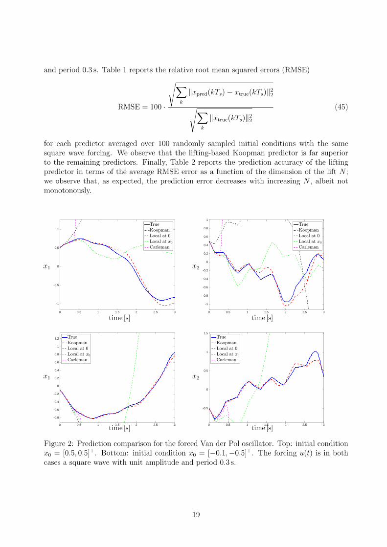
and period 0.3 s. Table 1 reports the relative root mean squared errors (RMSE)

RMSE = 100 ·

√∑k

‖xpred(kTs)− xtrue(kTs)‖22√∑

k

‖xtrue(kTs)‖22

(45)

for each predictor averaged over 100 randomly sampled initial conditions with the samesquare wave forcing. We observe that the lifting-based Koopman predictor is far superiorto the remaining predictors. Finally, Table 2 reports the prediction accuracy of the liftingpredictor in terms of the average RMSE error as a function of the dimension of the lift N ;we observe that, as expected, the prediction error decreases with increasing N , albeit notmonotonously.

0 0.5 1 1.5 2 2.5 3

-1

-0.5

0

0.5

1TrueKoopmanLocal at 0Local at x0

Carleman

0 0.5 1 1.5 2 2.5 3

-1

-0.8

-0.6

-0.4

-0.2

0

0.2

0.4

0.6

0.8

1

TrueKoopmanLocal at 0Local at x0

Carleman

0 0.5 1 1.5 2 2.5 3

-0.8

-0.6

-0.4

-0.2

0

0.2

0.4

0.6

0.8

1

1.2 TrueKoopmanLocal at 0Local at x0

Carleman

0 0.5 1 1.5 2 2.5 3

-0.5

0

0.5

1

1.5TrueKoopmanLocal at 0Local at x0

Carleman

time [s] time [s]

x1 x2

time [s] time [s]

x1 x2

Figure 2: Prediction comparison for the forced Van der Pol oscillator. Top: initial conditionx0 = [0.5, 0.5]>. Bottom: initial condition x0 = [−0.1,−0.5]>. The forcing u(t) is in bothcases a square wave with unit amplitude and period 0.3 s.

19

Table 1: Prediction comparison – average RMSE (45) over 100 randomly sampled initial conditions:comparison among different predictors.

x0 Average RMSE

Koopman 24.4 %

Local linearization at x0 2.83 · 103 %

Local linearization at 0 912.5 %

Carleman 5.08 · 1022 %

Table 2: Prediction comparison – lifting-based Koopman predictor – average prediction RMSEover 100 randomly sampled initial conditions as a function of the dimension of the lift.

N 5 10 25 50 75 100

Average RMSE 66.5 % 44.9 % 47.0 % 38.7 % 30.6 % 24.4 %

8.2 Feedback control of a bilinear motor

In this section we apply the proposed approach to the control of a bilinear model of a DCmotor [5]. The model reads

x1 = −(Ra/La)x1 − (km/La)x2u+ ua/La

x2 = −(B/J)x2 + (km/J)x1u− τl/J,y = x2

where x1 is the rotor current, x2 the angular velocity and the control input u is the statorcurrent and the output y is the angular velocity. The parameters are La = 0.314, Ra =12.345, km = 0.253, J = 0.00441, B = 0.00732, τl = 1.47, ua = 60. Notice in particular thebilinearity between the state and the control input. The physical constraints on the controlinput are u ∈ [−4, 4], which we scale to [−1, 1].

The goal is to design an MPC controller based on Section 7.1.2, i.e., assuming only input-output data available and no explicit knowledge of the model. In order to obtain the lifting-based predictor (39), we discretize the scaled dynamics using the Runge-Kutta four methodwith discretization period Ts = 0.01 s and simulate 200 trajectories over 1000 samplingperiods (i.e., 20 s per trajectory). The control input for each trajectory is a random signaluniformly distributed on [−1, 1]. The trajectories start from initial conditions generatedrandomly with uniform distribution on the unit box [−1, 1]2. We choose the number ofdelays nd = 1. The lifting functions ψi are chosen to be the time-delayed vector ζ ∈R3, defined in (36), and 100 thin plate spline radial basis functions (see Footnote 5) withcenters selected randomly with uniform distribution over [−1, 1]3. The dimension of thelifted state-space is therefore N = 103. First, in Figure 3, we compare the output predictionsfor two different, randomly chosen, initial conditions against the predictor based on locallinearization at a given initial condition. The prediction accuracy of the proposed predictoris superior, especially for longer prediction times. This is documented further in Table 3

20

by the relative root mean-squared errors (45) over a one-second prediction horizon averagedover one hundred randomly sampled initial conditions. Both in Figure 3 and Table 3, thecontrol signal was a pseudo-random binary signal generated anew for each initial condition.

Table 3: Feedback control of a bilinear motor – prediction RMSE (45) for 100 randomly generatedinitial condtions.

Koopman Local linearization at x0

Average RMSE 32.3 % 135.5 %

0 0.2 0.4 0.6 0.8 1

-1

-0.5

0

0.5

1 TrueKoopmanLocal at x0

0 0.2 0.4 0.6 0.8 1

-1

-0.5

0

0.5TrueKoopmanLocal at x0

time[s] time[s]

y y

Figure 3: Feedback control – predictor comparison for the bilinear motor model. Left: initialcondition x0 = [0.887, 0.587]>. Right: initial condition x0 = [−0.404,−0.126]>.

The control objective is to track a given angular velocity reference yr, which translates intothe objective function minimized in the MPC problem

J = (CzNp − yr)>QNp(CzNp − yr)

+

Np−1∑i=0

(Czi − yr)>Q(Czi − yr) + u>i Rui (46)

with C = [1, 0, . . . , 0]. This tracking objective function readily translates to the canonicalform (23) by expanding the quadratic forms and neglecting constant terms. The cost functionmatrices were chosen as Q = QNp = 1 and R = 0.01. The prediction horizon was set toone second, which results in Np = 100. We compare the Koopman operator-based MPCcontroller (K-MPC) with an MPC controller based on local linearization (L-MPC) in twoscenarios. In the first one we do not impose any constraints on the output and track apiecewise constant reference. In the second one, we impose the constraint y ∈ [−0.4, 0.4] andtrack a time-varying reference yr(t) = 0.5 cos(2πt/3), which violates the output constraintfor some portion of the simulated period. The simulation results are shown in Figure 4.We observe a virtually identical tracking performance in the first case. In the second case,however, the local-linearization controller becomes infeasible and hence cannot complete

21

0 0.5 1 1.5 2 2.5 3

-0.6

-0.4

-0.2

0

0.2

0.4

0.6

K-MPCL-MPCReference

0 1 2 3

-1

-0.5

0

0.5

1

K-MPCL-MPCConstraints

0 0.5 1 1.5 2 2.5 3

-0.4

-0.2

0

0.2

0.4

0.6K-MPCL-MPCReferenceConstraints

0 1 2 3

0

0.2

0.4

0.6

0.8

1

K-MPCL-MPCConstraint

0 0.05 0.1 0.15 0.2

0.2

0.4

0.6

0.8

1

CCCCCCO

L-MPCinfeasible

HHY

time[s] time[s]

y u

time[s] time[s]

y u

Figure 4: Feedback control – reference tracking for a bilinear model of a DC motor. Top:piecewise constant reference, x0 = [0, 0.6]>, no state constraints. Right: time-varying reference,x0 = [−0.1, 0.1]>, constraints on the output imposed.

the entire simulation period6. This infeasibility occurs due to the inaccurate predictionsof the local linearization predictor over longer prediction horizons. The proposed K-MPCcontroller, on the other hand, does not run infeasible and completes the simulation periodwithout violating the constraints.

Note that, even in the first scenario where the two controllers perform equally, the K-MPCcontroller has the benefit of being completely data-driven and requiring only output measure-ments, whereas the L-MPC controller requires a model (to compute the local linearization)and full state measurements. In addition, the average computation time7 required to evalu-ate the control input of the K-MPC controller was 6.86 ms (including the evaluation of thelifting mapping ψ(ζ)), as opposed to 103 ms for the L-MPC controller. This discrepancy isdue to the fact that the local linearization and all data defining the underlying optimizationproblem that depend on it have to be re-computed at every iteration, which is costly on itsown and also precludes efficient warm-starting; on the other hand, all data (except for theinitial condition) of the underlying optimization problem of K-MPC are precomputed offline.In both cases, the computation times could be significantly reduced with a more efficient

6Infeasibility of the underlying optimization problem is a common problem encountered in predictivecontrol with various heuristic (e.g., soft constraints) or theoretically substantiated (e.g., set invariance)approaches trying to address them. See, e.g., [7, 19] for more details.

7The optimization problems were solved by qpOASES [6] running on Matlab and 2 GHz Intel Core i7with 8 GB RAM.

22

implementation. However, we believe, that the proposed approach would still be superior interms of computational speed.

8.3 Nonlinear PDE control

In order to demonstrate the scalability and versatility of the approach, we use it to controlthe nonlinear Korteweg-de Vries (KdV) equation modelling the propagation of acoustic wavesin a plasma or shallow-water waves [16]. The equation reads

∂ y(t, x)

∂t+ y(t, x)

∂y(t, x)

∂x+∂3y(t, x)

∂x3= u(t, x),

where y(t, x) is the unknown function and u(t, x) the control input. We consider a periodicboundary condition on the spatial variable x ∈ [−π, π]. The nonlinear PDE is discretizedusing the split-stepping method with spatial mesh of 128 points and time discretization of∆t = 0.01 s, resulting in a computational state-space of dimension n = 128. The control in-put u is considered to be of the form u(t, x) =

∑3i=1 ui(t)vi(x), where the coefficients ui(t) are

to be determined by the controller and vi are fixed spatial profiles given by vi(x) = e−25(x−ci)2

with c1 = −π/2, c2 = 0, c3 = π/2. The control inputs are constrained to ui(t) ∈ [−1, 1]. Thelifting-based predictors are constructed from data in the form of 1000 trajectories of length200 samples. The initial conditions of the trajectories are random convex combinations ofthree fixed spatial profiles given by y1

0 = e−(x−π/2)2 , y20 = − sin(x/2)2, y3

0 = e−(x+π/2)2 ; thecontrol inputs ui(t) are distributed uniformly in [−1, 1]3. The lifting mapping ψ is composedof the state itself, the elementwise square of the state, the elementwise product of the statewith its periodic shift and the constant function, resulting in the dimension of the liftedstate N = 3 · 128 + 1 = 385. The control goal is to track a constant-in-space reference thatvaries in time in a piecewise constant manner. In order to do so we design the lifting-basedKoopman MPC (23) with the reference tracking objective (46) with Q = QNp = I, R = 0,C = [I128, 0] and prediction horizon Np = 10 (i.e., 0.1 s). The results are depicted in Figure 5;we observe a fast and accurate tracking of the reference profile. The average computationtime to evaluate the control input was 0.28 ms (using the dense form (24) and the hardwareconfiguration described in Footnote 7), allowing for deployment in applications requiring fastsampling rates such as tokamak control.

9 Conclusion and outlook

In this paper, we described a class of linear predictors for nonlinear controlled dynamicalsystems building on the Koopman operator framework. The underlying idea is to lift thenonlinear dynamics to a higher dimensional space where its evolution is approximately linear.The predictors exhibit superior performance on the numerical examples tested and can bereadily used for feedback control design using linear control design methods. In particular,linear model predictive control (MPC) can be readily used to design controllers for thenonlinear dynamical system without resorting to non-linear numerical optimization schemes.Linear inequality constraints on the states and control inputs as well as nonlinear constraintson the states can be imposed in a linear fashion; in addition cost functions nonlinear in the

23

0 10 20 30 40 50-0.1

0

0.1

0.2

0.3

0.4

0.5

0.6

0.7

0.8Spatial mean of y(t; x)Reference

0 10 20 30 40 50-1

-0.8

-0.6

-0.4

-0.2

0

0.2

0.4

0.6

0.8

1u1(t)u2(t)u3(t)

xt[s]

y(t,x

)

t[s] t [s]

Figure 5: Nonlinear PDE control – Tracking of a time-varying constant-in-space profile for theKdV equation. Left: closed-loop solution. Middle: spatial mean of the solution. Right: controlinputs.

state can be handled in a linear fashion as well. Computational complexity of the underlyingoptimization problem is comparable to that of an MPC problem for a linear dynamicalsystem of the same size. This is achieved by using the so-called dense form of an MPCproblem whose computational complexity depends only on the number of control inputsand is virtually independent of the number of states. Importantly, the entire control designprocedure is data-driven, requiring only input-output measurements.

Future work should focus on imposing or proving closed-loop guarantees (e.g., stability ordegree of suboptimality) of the controller designed using the presented methodology andon optimal selection of the lifting functions given some prior information on the dynamicalsystem at hand.

10 Acknowledgments

The first author would like to thank Colin N. Jones for initial discussions on the topicand for comments on the manuscript, as well as to the three anonymous referees for theirconstructive comments that helped improve the manuscript. The authors would also like tothank Peter Koltai for bringing to our attantion reference [8].

This research was supported in part by the ARO-MURI grant W911NF-14-1-0359 and theDARPA grant HR0011-16-C-0116. The research of M. Korda was supported by the SwissNational Science Foundation under grant P2ELP2 165166.

Appendix

This appendix expresses explicitly the matrices in the “dense-form” MPC problem (24) as afunction of the data defining the “sparse-form” MPC problem (23). The matrices are givenby

H = R + B>QB, h = q>B + r>, G = 2A>QB,

L = F + EB, M = EA, c = [b>0 , . . . , b>Np ]>,

24

where

A =

IAA2

...ANp

, B =

0 0 . . . 0B 0 . . . 0AB B . . . 0

.... . . . . .

ANp−1B . . . AB B

, F =

F0 0 . . . 00 F1 . . . 0...

. . ....

0 0 . . . FNp−1

0 0 . . . 0

Q = diag(Q0, . . . , QNp), R = diag(R0, . . . , RNp−1),

E = diag(E0, . . . , ENp), q = [q0, . . . , qNp ], r = [r0, . . . , rNp−1],

with diag(·, . . . , ·) denoting a block-diagonal matrix composed of the arguments.

References

[1] S. L. Brunton, B. W. Brunton, J. L. Proctor, E. Kaiser, and J. N. Kutz. Chaos as anintermittently forced linear system. arXiv preprint arXiv:1608.05306, 2016.

[2] S. L. Brunton, B. W. Brunton, J. L. Proctor, and J. N. Kutz. Koopman invariantsubspaces and finite linear representations of nonlinear dynamical systems for control.PloS one, 11(2):e0150171, 2016.

[3] M. Budisic, R. Mohr, and I. Mezic. Applied Koopmanism. Chaos: An InterdisciplinaryJournal of Nonlinear Science, 22(4):047510, 2012.

[4] T. Carleman. Application de la theorie des equations integrales lineaires aux systemesd’equations differentielles non lineaires. Acta Mathematica, 59(1):63–87, 1932.

[5] S. Daniel-Berhe and H. Unbehauen. Experimental physical parameter estimation ofa thyristor driven DC-motor using the HMF-method. Control Engineering Practice,6(5):615–626, 1998.

[6] H. J. Ferreau, C. Kirches, A. Potschka, H. G. Bock, and M. Diehl. qpOASES: Aparametric active-set algorithm for quadratic programming. Mathematical ProgrammingComputation, 6(4):327–363, 2014.

[7] L. Grune and J. Pannek. Nonlinear model predictive control. In Nonlinear ModelPredictive Control. Springer, 2011.

[8] S. Klus, P. Koltai, and C. Schutte. On the numerical approximation of the Perron-Frobenius and Koopman operator. Journal of Computational Dynamics, 3(1):51–79,2016.

[9] B. Koopman. Hamiltonian systems and transformation in Hilbert space. Proceedingsof the National Academy of Sciences of the United States of America, 17(5):315–318,1931.

25

[10] B. Koopman and J. von Neuman. Dynamical systems of continuous spectra. Proceedingsof the National Academy of Sciences of the United States of America, 18(3):255–263,1932.

[11] M. Korda and I. Mezic. On convergence of Extended dynamic mode decomposition tothe Koopman operator. arXiv preprint: arXiv:1703.04680, 2017.

[12] L. Ljung. System identification. In Signal Analysis and Prediction, pages 163–173.Springer, 1998.

[13] A. Mauroy and J. Goncalves. Linear identification of nonlinear systems: A liftingtechnique based on the Koopman operator. In Conference on Decision and Control(CDC), 2016.

[14] D. Q. Mayne, J. B. Rawlings, C. V. Rao, and P. O. Scokaert. Constrained modelpredictive control: Stability and optimality. Automatica, 36(6):789–814, 2000.

[15] I. Mezic. Spectral properties of dynamical systems, model reduction and decomposi-tions. Nonlinear Dynamics, 41(1-3):309–325, 2005.

[16] R. M. Miura. The korteweg–devries equation: A survey of results. SIAM review,18(3):412–459, 1976.

[17] J. L. Proctor, S. L. Brunton, and J. N. Kutz. Dynamic mode decomposition withcontrol. SIAM Journal on Applied Dynamical Systems, 15(1):142–161, 2016.

[18] J. L. Proctor, S. L. Brunton, and J. N. Kutz. Generalizing Koopman theory to allowfor inputs and control. arXiv preprint arXiv:1602.07647, 2016.

[19] J. B. Rawlings and D. Q. Mayne. Model Predictive Control: Theory and Design. NobHill Publishing, first edition, 2009.

[20] A. Surana. Koopman operator based observer synthesis for control-affine nonlinearsystems. In Conference on Decision and Control (CDC), 2016.

[21] A. Surana and A. Banaszuk. Linear observer synthesis for nonlinear systems usingKoopman operator framework. In IFAC Symposium on Nonlinear Control Systems(NOLCOS), 2016.

[22] J. H. Tu, C. W. Rowley, D. M. Luchtenburg, S. L. Brunton, and J. N. Kutz. On dynamicmode decomposition: theory and applications. arXiv preprint arXiv:1312.0041, 2013.

[23] M. O. Williams, M. S. Hemati, S. T. M. Dawson, I. G. Kevrekidis, and C. W. Rowley.Extending data-driven Koopman analysis to actuated systems. In IFAC Symposium onNonlinear Control Systems (NOLCOS), 2016.

[24] M. O. Williams, I. G. Kevrekidis, and C. W. Rowley. A data–driven approximation ofthe Koopman operator: Extending dynamic mode decomposition. Journal of NonlinearScience, 25(6):1307–1346, 2015.

[25] M. O. Williams, C. W. Rowley, and I. G. Kevrekidis. A kernel-based approach todata-driven Koopman spectral analysis. arXiv preprint arXiv:1411.2260, 2014.

26