Embed Size (px)
Citation preview
IntroductionMethodology
Simulation studyMacroeconomic application
Conclusions
Nonlinear Forecasting with Many Predictorsusing Kernel Ridge Regression
Peter Exterkate
Seventh ECB Workshop on Forecasting TechniquesNew Directions for Forecasting
Frankfurt am Main, May 4, 2012
Peter Exterkate (CREATES, Aarhus University) Nonlinear Forecasting with Many Predictors using Kernel Ridge Regression

IntroductionMethodology
Simulation studyMacroeconomic application
Conclusions
One-slide summary
I Main research question: Is it possible to forecast with large datasets, while allowing for nonlinear relations between target variableand predictors?
I Background: Large data sets are increasingly available inmacroeconomics and finance, but forecasting is mostly limited to alinear framework
I Solution: Kernel ridge regression (KRR), which avoids the curse ofdimensionality by manipulating the forecast equation in a clever way:the kernel trick
I Contributions:
I Extension of KRR to models with “preferred” predictorsI Monte Carlo and empirical evidence that KRR works, and improves
upon conventional techniques such as principal component regressionI Clearer understanding of the choice of kernel and tuning parameters
(companion paper)
I Joint work with Patrick Groenen, Christiaan Heij, and Dick van Dijk(Econometric Institute, Erasmus University Rotterdam)
Peter Exterkate (CREATES, Aarhus University) Nonlinear Forecasting with Many Predictors using Kernel Ridge Regression

IntroductionMethodology
Simulation studyMacroeconomic application
Conclusions
One-slide summary
I Main research question: Is it possible to forecast with large datasets, while allowing for nonlinear relations between target variableand predictors?
I Background: Large data sets are increasingly available inmacroeconomics and finance, but forecasting is mostly limited to alinear framework
I Solution: Kernel ridge regression (KRR), which avoids the curse ofdimensionality by manipulating the forecast equation in a clever way:the kernel trick
I Contributions:I Extension of KRR to models with “preferred” predictorsI Monte Carlo and empirical evidence that KRR works, and improves
upon conventional techniques such as principal component regressionI Clearer understanding of the choice of kernel and tuning parameters
(companion paper)I Joint work with Patrick Groenen, Christiaan Heij, and Dick van Dijk
(Econometric Institute, Erasmus University Rotterdam)Peter Exterkate (CREATES, Aarhus University) Nonlinear Forecasting with Many Predictors using Kernel Ridge Regression

IntroductionMethodology
Simulation studyMacroeconomic application
Conclusions
Introduction
I How to forecast in today’s data-rich environment?
I In an ideal world:
I use all available informationI flexible functional forms
I In practice:
I the simpler the betterI “curse of dimensionality”
Peter Exterkate (CREATES, Aarhus University) Nonlinear Forecasting with Many Predictors using Kernel Ridge Regression

IntroductionMethodology
Simulation studyMacroeconomic application
Conclusions
Introduction
I How to forecast in today’s data-rich environment?
I In an ideal world:I use all available informationI flexible functional forms
I In practice:I the simpler the betterI “curse of dimensionality”
Peter Exterkate (CREATES, Aarhus University) Nonlinear Forecasting with Many Predictors using Kernel Ridge Regression

IntroductionMethodology
Simulation studyMacroeconomic application
Conclusions
Possible ways out
I Handling high-dimensionality:
I Principal components regression (Stock and Watson, 2002)I Partial least squares (Groen and Kapetanios, 2008)I Selecting variables (Bai and Ng, 2008)I Bayesian regression (De Mol, Giannone, Reichlin, 2008)
I Handling nonlinearity:
I Neural networks (Terasvirta, Van Dijk, Medeiros, 2005)I Linear regression on nonlinear PCs (Bai and Ng, 2008)I Nonlinear regression on linear PCs (Giovannetti, 2011)
I Unified approach: kernel ridge regression
Peter Exterkate (CREATES, Aarhus University) Nonlinear Forecasting with Many Predictors using Kernel Ridge Regression

IntroductionMethodology
Simulation studyMacroeconomic application
Conclusions
Possible ways out
I Handling high-dimensionality:I Principal components regression (Stock and Watson, 2002)
I Partial least squares (Groen and Kapetanios, 2008)I Selecting variables (Bai and Ng, 2008)I Bayesian regression (De Mol, Giannone, Reichlin, 2008)
I Handling nonlinearity:
I Neural networks (Terasvirta, Van Dijk, Medeiros, 2005)I Linear regression on nonlinear PCs (Bai and Ng, 2008)I Nonlinear regression on linear PCs (Giovannetti, 2011)
I Unified approach: kernel ridge regression
Peter Exterkate (CREATES, Aarhus University) Nonlinear Forecasting with Many Predictors using Kernel Ridge Regression

IntroductionMethodology
Simulation studyMacroeconomic application
Conclusions
Possible ways out
I Handling high-dimensionality:I Principal components regression (Stock and Watson, 2002)I Partial least squares (Groen and Kapetanios, 2008)
I Selecting variables (Bai and Ng, 2008)I Bayesian regression (De Mol, Giannone, Reichlin, 2008)
I Handling nonlinearity:
I Neural networks (Terasvirta, Van Dijk, Medeiros, 2005)I Linear regression on nonlinear PCs (Bai and Ng, 2008)I Nonlinear regression on linear PCs (Giovannetti, 2011)
I Unified approach: kernel ridge regression
Peter Exterkate (CREATES, Aarhus University) Nonlinear Forecasting with Many Predictors using Kernel Ridge Regression

IntroductionMethodology
Simulation studyMacroeconomic application
Conclusions
Possible ways out
I Handling high-dimensionality:I Principal components regression (Stock and Watson, 2002)I Partial least squares (Groen and Kapetanios, 2008)I Selecting variables (Bai and Ng, 2008)
I Bayesian regression (De Mol, Giannone, Reichlin, 2008)
I Handling nonlinearity:
I Neural networks (Terasvirta, Van Dijk, Medeiros, 2005)I Linear regression on nonlinear PCs (Bai and Ng, 2008)I Nonlinear regression on linear PCs (Giovannetti, 2011)
I Unified approach: kernel ridge regression
Peter Exterkate (CREATES, Aarhus University) Nonlinear Forecasting with Many Predictors using Kernel Ridge Regression

IntroductionMethodology
Simulation studyMacroeconomic application
Conclusions
Possible ways out
I Handling high-dimensionality:I Principal components regression (Stock and Watson, 2002)I Partial least squares (Groen and Kapetanios, 2008)I Selecting variables (Bai and Ng, 2008)I Bayesian regression (De Mol, Giannone, Reichlin, 2008)
I Handling nonlinearity:I Neural networks (Terasvirta, Van Dijk, Medeiros, 2005)
I Linear regression on nonlinear PCs (Bai and Ng, 2008)I Nonlinear regression on linear PCs (Giovannetti, 2011)
I Unified approach: kernel ridge regression
Peter Exterkate (CREATES, Aarhus University) Nonlinear Forecasting with Many Predictors using Kernel Ridge Regression

IntroductionMethodology
Simulation studyMacroeconomic application
Conclusions
Possible ways out
I Handling high-dimensionality:I Principal components regression (Stock and Watson, 2002)I Partial least squares (Groen and Kapetanios, 2008)I Selecting variables (Bai and Ng, 2008)I Bayesian regression (De Mol, Giannone, Reichlin, 2008)
I Handling nonlinearity:I Neural networks (Terasvirta, Van Dijk, Medeiros, 2005)I Linear regression on nonlinear PCs (Bai and Ng, 2008)
I Nonlinear regression on linear PCs (Giovannetti, 2011)
I Unified approach: kernel ridge regression
Peter Exterkate (CREATES, Aarhus University) Nonlinear Forecasting with Many Predictors using Kernel Ridge Regression

IntroductionMethodology
Simulation studyMacroeconomic application
Conclusions
Possible ways out
I Handling high-dimensionality:I Principal components regression (Stock and Watson, 2002)I Partial least squares (Groen and Kapetanios, 2008)I Selecting variables (Bai and Ng, 2008)I Bayesian regression (De Mol, Giannone, Reichlin, 2008)
I Handling nonlinearity:I Neural networks (Terasvirta, Van Dijk, Medeiros, 2005)I Linear regression on nonlinear PCs (Bai and Ng, 2008)I Nonlinear regression on linear PCs (Giovannetti, 2011)
I Unified approach: kernel ridge regression
Peter Exterkate (CREATES, Aarhus University) Nonlinear Forecasting with Many Predictors using Kernel Ridge Regression

IntroductionMethodology
Simulation studyMacroeconomic application
Conclusions
Forecasting context
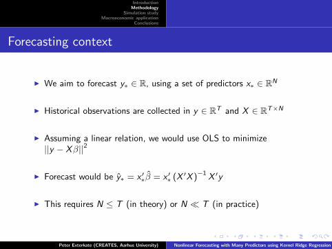
I We aim to forecast y∗ ∈ R, using a set of predictors x∗ ∈ RN
I Historical observations are collected in y ∈ RT and X ∈ RT×N
I Assuming a linear relation, we would use OLS to minimize||y − Xβ||2
I Forecast would be y∗ = x ′∗β = x ′∗ (X ′X )−1
X ′y
I This requires N ≤ T (in theory) or N � T (in practice)
Peter Exterkate (CREATES, Aarhus University) Nonlinear Forecasting with Many Predictors using Kernel Ridge Regression
IntroductionMethodology
Simulation studyMacroeconomic application
Conclusions
Forecasting context
I We aim to forecast y∗ ∈ R, using a set of predictors x∗ ∈ RN
I Historical observations are collected in y ∈ RT and X ∈ RT×N
I Assuming a linear relation, we would use OLS to minimize||y − Xβ||2
I Forecast would be y∗ = x ′∗β = x ′∗ (X ′X )−1
X ′y
I This requires N ≤ T (in theory) or N � T (in practice)
Peter Exterkate (CREATES, Aarhus University) Nonlinear Forecasting with Many Predictors using Kernel Ridge Regression

IntroductionMethodology
Simulation studyMacroeconomic application
Conclusions
Ridge regression
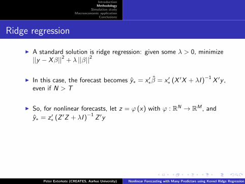
I A standard solution is ridge regression: given some λ > 0, minimize||y − Xβ||2 + λ ||β||2
I In this case, the forecast becomes y∗ = x ′∗β = x ′∗ (X ′X + λI )−1
X ′y ,even if N > T
I So, for nonlinear forecasts, let z = ϕ (x) with ϕ : RN → RM , and
y∗ = z ′∗ (Z ′Z + λI )−1 Z ′y
I For very large M, the inversion is numerically unstable andcomputationally intensive
I Typical example: N = 132, quadratic model ⇒ M = 8911
Peter Exterkate (CREATES, Aarhus University) Nonlinear Forecasting with Many Predictors using Kernel Ridge Regression

IntroductionMethodology
Simulation studyMacroeconomic application
Conclusions
Ridge regression
I A standard solution is ridge regression: given some λ > 0, minimize||y − Xβ||2 + λ ||β||2
I In this case, the forecast becomes y∗ = x ′∗β = x ′∗ (X ′X + λI )−1
X ′y ,even if N > T
I So, for nonlinear forecasts, let z = ϕ (x) with ϕ : RN → RM , and
y∗ = z ′∗ (Z ′Z + λI )−1 Z ′y
I For very large M, the inversion is numerically unstable andcomputationally intensive
I Typical example: N = 132, quadratic model ⇒ M = 8911
Peter Exterkate (CREATES, Aarhus University) Nonlinear Forecasting with Many Predictors using Kernel Ridge Regression

IntroductionMethodology
Simulation studyMacroeconomic application
Conclusions
Kernel trick (Boser, Guyon, Vapnik, 1992)
I Essential idea: if M � T , working with T -dimensional objects iseasier than working with M-dimensional objects
I We wish to compute y∗ = z ′∗ (Z ′Z + λI )−1 Z ′y
I Some algebra yields y∗ = z ′∗Z′ (ZZ ′ + λI )−1 y
I So if we know k∗ = Zz∗ ∈ RT and K = ZZ ′ ∈ RT×T , computingy∗ = k ′∗ (K + λI )−1 y is feasible
I Define the kernel function κ (xs , xt) = ϕ (xs)′ ϕ (xt)
I tth element of k∗ is z ′tz∗ = κ (xt , x∗)I (s, t)th element of K is z ′szt = κ (xs , xt)
I If we choose ϕ smartly, κ (and hence y∗) will be easy to compute!
Peter Exterkate (CREATES, Aarhus University) Nonlinear Forecasting with Many Predictors using Kernel Ridge Regression

IntroductionMethodology
Simulation studyMacroeconomic application
Conclusions
Kernel trick (Boser, Guyon, Vapnik, 1992)
I Essential idea: if M � T , working with T -dimensional objects iseasier than working with M-dimensional objects
I We wish to compute y∗ = z ′∗ (Z ′Z + λI )−1 Z ′y
I Some algebra yields y∗ = z ′∗Z′ (ZZ ′ + λI )−1 y
I So if we know k∗ = Zz∗ ∈ RT and K = ZZ ′ ∈ RT×T , computingy∗ = k ′∗ (K + λI )−1 y is feasible
I Define the kernel function κ (xs , xt) = ϕ (xs)′ ϕ (xt)I tth element of k∗ is z ′tz∗ = κ (xt , x∗)I (s, t)th element of K is z ′szt = κ (xs , xt)
I If we choose ϕ smartly, κ (and hence y∗) will be easy to compute!
Peter Exterkate (CREATES, Aarhus University) Nonlinear Forecasting with Many Predictors using Kernel Ridge Regression

IntroductionMethodology
Simulation studyMacroeconomic application
Conclusions
Bayesian interpretation
I Like “normal” ridge regression, KRR has a Bayesian interpretation:
I Likelihood: p(y |X , β, θ2
)= N
(Zβ, θ2I
)I Priors: p
(θ2)∝ θ−2, p (β|θ) = N
(0,(θ2/λ
)I)
I Posterior distribution of y∗ is Student’s t with T degrees of freedom,mode y∗, variance also analytically available
I Note that we can interpret λ in terms of the signal-to-noise ratio
Peter Exterkate (CREATES, Aarhus University) Nonlinear Forecasting with Many Predictors using Kernel Ridge Regression

IntroductionMethodology
Simulation studyMacroeconomic application
Conclusions
Bayesian interpretation
I Like “normal” ridge regression, KRR has a Bayesian interpretation:
I Likelihood: p(y |X , β, θ2
)= N
(Zβ, θ2I
)
I Priors: p(θ2)∝ θ−2, p (β|θ) = N
(0,(θ2/λ
)I)
I Posterior distribution of y∗ is Student’s t with T degrees of freedom,mode y∗, variance also analytically available
I Note that we can interpret λ in terms of the signal-to-noise ratio
Peter Exterkate (CREATES, Aarhus University) Nonlinear Forecasting with Many Predictors using Kernel Ridge Regression

IntroductionMethodology
Simulation studyMacroeconomic application
Conclusions
Bayesian interpretation
I Like “normal” ridge regression, KRR has a Bayesian interpretation:
I Likelihood: p(y |X , β, θ2
)= N
(Zβ, θ2I
)I Priors: p
(θ2)∝ θ−2, p (β|θ) = N
(0,(θ2/λ
)I)
I Posterior distribution of y∗ is Student’s t with T degrees of freedom,mode y∗, variance also analytically available
I Note that we can interpret λ in terms of the signal-to-noise ratio
Peter Exterkate (CREATES, Aarhus University) Nonlinear Forecasting with Many Predictors using Kernel Ridge Regression

IntroductionMethodology
Simulation studyMacroeconomic application
Conclusions
Bayesian interpretation
I Like “normal” ridge regression, KRR has a Bayesian interpretation:
I Likelihood: p(y |X , β, θ2
)= N
(Zβ, θ2I
)I Priors: p
(θ2)∝ θ−2, p (β|θ) = N
(0,(θ2/λ
)I)
I Posterior distribution of y∗ is Student’s t with T degrees of freedom,mode y∗, variance also analytically available
I Note that we can interpret λ in terms of the signal-to-noise ratio
Peter Exterkate (CREATES, Aarhus University) Nonlinear Forecasting with Many Predictors using Kernel Ridge Regression

IntroductionMethodology
Simulation studyMacroeconomic application
Conclusions
Function approximation (Hofmann, Scholkopf, Smola, 2008)
I Other way to look at KRR: it also solves, for some Hilbert space H,
minf∈H
T∑t=1
(yt − f (xt))2 + λ ||f ||2H
I Choosing a kernel function implies choosing H and its norm ||·||H
I The “complexity” of the prediction function is measured by ||f ||H
Peter Exterkate (CREATES, Aarhus University) Nonlinear Forecasting with Many Predictors using Kernel Ridge Regression
IntroductionMethodology
Simulation studyMacroeconomic application
Conclusions
Choosing the kernel function
I We can understand KRR from a Bayesian/ridge point of view, or asa function approximation technique
I Thus, our choice of kernel can be guided in two ways:
I The prediction function x 7→ y will be linear in ϕ (x), so choose a κthat leads to a ϕ for which this makes sense
I Complexity of the prediction function is penalized through ||·||H, sochoose a κ for which this penalty ensures “smoothness”
I We will give examples of both
Peter Exterkate (CREATES, Aarhus University) Nonlinear Forecasting with Many Predictors using Kernel Ridge Regression

IntroductionMethodology
Simulation studyMacroeconomic application
Conclusions
Choosing the kernel function
I We can understand KRR from a Bayesian/ridge point of view, or asa function approximation technique
I Thus, our choice of kernel can be guided in two ways:I The prediction function x 7→ y will be linear in ϕ (x), so choose a κ
that leads to a ϕ for which this makes sense
I Complexity of the prediction function is penalized through ||·||H, sochoose a κ for which this penalty ensures “smoothness”
I We will give examples of both
Peter Exterkate (CREATES, Aarhus University) Nonlinear Forecasting with Many Predictors using Kernel Ridge Regression

IntroductionMethodology
Simulation studyMacroeconomic application
Conclusions
Choosing the kernel function
I We can understand KRR from a Bayesian/ridge point of view, or asa function approximation technique
I Thus, our choice of kernel can be guided in two ways:I The prediction function x 7→ y will be linear in ϕ (x), so choose a κ
that leads to a ϕ for which this makes senseI Complexity of the prediction function is penalized through ||·||H, so
choose a κ for which this penalty ensures “smoothness”
I We will give examples of both
Peter Exterkate (CREATES, Aarhus University) Nonlinear Forecasting with Many Predictors using Kernel Ridge Regression

IntroductionMethodology
Simulation studyMacroeconomic application
Conclusions
Polynomial kernel functions (Poggio, 1975)
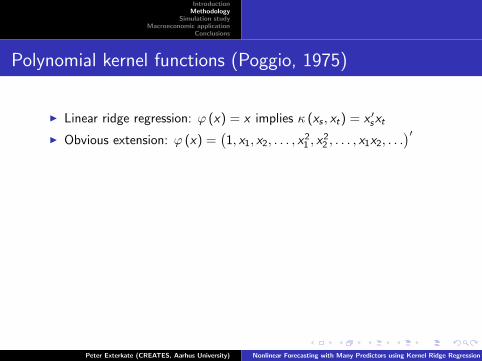
I Linear ridge regression: ϕ (x) = x implies κ (xs , xt) = x ′sxt
I Obvious extension: ϕ (x) =(1, x1, x2, . . . , x
21 , x
22 , . . . , x1x2, . . .
)′I However, κ does not take a particularly simple form in this case
I Better: ϕ (x) =(
1,√2σ x1,
√2σ x2, . . . ,
1σ2 x2
1 ,1σ2 x2
2 , . . . ,√2
σ2 x1x2, . . .)′
,
which implies κ (xs , xt) =(
1 +x′s xtσ2
)2I More generally, κ (xs , xt) =
(1 +
x′s xtσ2
)dcorresponds to
ϕ (x) = (all monomials in x up to degree d)
I Interpretation of tuning parameter: higher σ ⇒ smaller coefficientson higher-order terms ⇒ smoother prediction function
Peter Exterkate (CREATES, Aarhus University) Nonlinear Forecasting with Many Predictors using Kernel Ridge Regression

IntroductionMethodology
Simulation studyMacroeconomic application
Conclusions
Polynomial kernel functions (Poggio, 1975)
I Linear ridge regression: ϕ (x) = x implies κ (xs , xt) = x ′sxt
I Obvious extension: ϕ (x) =(1, x1, x2, . . . , x
21 , x
22 , . . . , x1x2, . . .
)′I However, κ does not take a particularly simple form in this case
I Better: ϕ (x) =(
1,√2σ x1,
√2σ x2, . . . ,
1σ2 x2
1 ,1σ2 x2
2 , . . . ,√2
σ2 x1x2, . . .)′
,
which implies κ (xs , xt) =(
1 +x′s xtσ2
)2I More generally, κ (xs , xt) =
(1 +
x′s xtσ2
)dcorresponds to
ϕ (x) = (all monomials in x up to degree d)
I Interpretation of tuning parameter: higher σ ⇒ smaller coefficientson higher-order terms ⇒ smoother prediction function
Peter Exterkate (CREATES, Aarhus University) Nonlinear Forecasting with Many Predictors using Kernel Ridge Regression
IntroductionMethodology
Simulation studyMacroeconomic application
Conclusions
Polynomial kernel functions (Poggio, 1975)
I Linear ridge regression: ϕ (x) = x implies κ (xs , xt) = x ′sxt
I Obvious extension: ϕ (x) =(1, x1, x2, . . . , x
21 , x
22 , . . . , x1x2, . . .
)′
I However, κ does not take a particularly simple form in this case
I Better: ϕ (x) =(
1,√2σ x1,
√2σ x2, . . . ,
1σ2 x2
1 ,1σ2 x2
2 , . . . ,√2
σ2 x1x2, . . .)′
,
which implies κ (xs , xt) =(
1 +x′s xtσ2
)2I More generally, κ (xs , xt) =
(1 +
x′s xtσ2
)dcorresponds to
ϕ (x) = (all monomials in x up to degree d)
I Interpretation of tuning parameter: higher σ ⇒ smaller coefficientson higher-order terms ⇒ smoother prediction function
Peter Exterkate (CREATES, Aarhus University) Nonlinear Forecasting with Many Predictors using Kernel Ridge Regression

IntroductionMethodology
Simulation studyMacroeconomic application
Conclusions
Polynomial kernel functions (Poggio, 1975)
I Linear ridge regression: ϕ (x) = x implies κ (xs , xt) = x ′sxt
I Obvious extension: ϕ (x) =(1, x1, x2, . . . , x
21 , x
22 , . . . , x1x2, . . .
)′I However, κ does not take a particularly simple form in this case
I Better: ϕ (x) =(
1,√2σ x1,
√2σ x2, . . . ,
1σ2 x2
1 ,1σ2 x2
2 , . . . ,√2
σ2 x1x2, . . .)′
,
which implies κ (xs , xt) =(
1 +x′s xtσ2
)2I More generally, κ (xs , xt) =
(1 +
x′s xtσ2
)dcorresponds to
ϕ (x) = (all monomials in x up to degree d)
I Interpretation of tuning parameter: higher σ ⇒ smaller coefficientson higher-order terms ⇒ smoother prediction function
Peter Exterkate (CREATES, Aarhus University) Nonlinear Forecasting with Many Predictors using Kernel Ridge Regression

IntroductionMethodology
Simulation studyMacroeconomic application
Conclusions
Polynomial kernel functions (Poggio, 1975)
I Linear ridge regression: ϕ (x) = x implies κ (xs , xt) = x ′sxt
I Obvious extension: ϕ (x) =(1, x1, x2, . . . , x
21 , x
22 , . . . , x1x2, . . .
)′I However, κ does not take a particularly simple form in this case
I Better: ϕ (x) =(
1,√2σ x1,
√2σ x2, . . . ,
1σ2 x2
1 ,1σ2 x2
2 , . . . ,√2
σ2 x1x2, . . .)′
,
which implies κ (xs , xt) =(
1 +x′s xtσ2
)2
I More generally, κ (xs , xt) =(
1 +x′s xtσ2
)dcorresponds to
ϕ (x) = (all monomials in x up to degree d)
I Interpretation of tuning parameter: higher σ ⇒ smaller coefficientson higher-order terms ⇒ smoother prediction function
Peter Exterkate (CREATES, Aarhus University) Nonlinear Forecasting with Many Predictors using Kernel Ridge Regression

IntroductionMethodology
Simulation studyMacroeconomic application
Conclusions
Polynomial kernel functions (Poggio, 1975)
I Linear ridge regression: ϕ (x) = x implies κ (xs , xt) = x ′sxt
I Obvious extension: ϕ (x) =(1, x1, x2, . . . , x
21 , x
22 , . . . , x1x2, . . .
)′I However, κ does not take a particularly simple form in this case
I Better: ϕ (x) =(
1,√2σ x1,
√2σ x2, . . . ,
1σ2 x2
1 ,1σ2 x2
2 , . . . ,√2
σ2 x1x2, . . .)′
,
which implies κ (xs , xt) =(
1 +x′s xtσ2
)2I More generally, κ (xs , xt) =
(1 +
x′s xtσ2
)dcorresponds to
ϕ (x) = (all monomials in x up to degree d)
I Interpretation of tuning parameter: higher σ ⇒ smaller coefficientson higher-order terms ⇒ smoother prediction function
Peter Exterkate (CREATES, Aarhus University) Nonlinear Forecasting with Many Predictors using Kernel Ridge Regression

IntroductionMethodology
Simulation studyMacroeconomic application
Conclusions
Polynomial kernel functions (Poggio, 1975)
I Linear ridge regression: ϕ (x) = x implies κ (xs , xt) = x ′sxt
I Obvious extension: ϕ (x) =(1, x1, x2, . . . , x
21 , x
22 , . . . , x1x2, . . .
)′I However, κ does not take a particularly simple form in this case
I Better: ϕ (x) =(
1,√2σ x1,
√2σ x2, . . . ,
1σ2 x2
1 ,1σ2 x2
2 , . . . ,√2
σ2 x1x2, . . .)′
,
which implies κ (xs , xt) =(
1 +x′s xtσ2
)2I More generally, κ (xs , xt) =
(1 +
x′s xtσ2
)dcorresponds to
ϕ (x) = (all monomials in x up to degree d)
I Interpretation of tuning parameter: higher σ ⇒ smaller coefficientson higher-order terms ⇒ smoother prediction function
Peter Exterkate (CREATES, Aarhus University) Nonlinear Forecasting with Many Predictors using Kernel Ridge Regression

IntroductionMethodology
Simulation studyMacroeconomic application
Conclusions
The Gaussian kernel function (Broomhead and Lowe, 1988)
I Examine the effects of ||f ||H on f , the Fourier transform of theprediction function. Popular choice: set the kernel κ such that
||f ||H ∝∫RN
∣∣∣f (ω)∣∣∣2
σN exp(− 1
2σ2ω′ω
)dω
I As σ ↑, components at high frequencies ω are penalized moreheavily, leading to a smoother f
I Corresponding kernel is κ (xs , xt) = exp(−12σ2 ||xs − xt ||2
)I For a ridge regression interpretation, we would need to build
infinitely many regressors of the form exp(− x′x
2σ2
)∏Nn=1
xdnn
σdn√dn!
, for
nonnegative integers d1, d2, . . . , dN . Thus, the kernel trick allows usto implicitly work with an infinite number of regressors
Peter Exterkate (CREATES, Aarhus University) Nonlinear Forecasting with Many Predictors using Kernel Ridge Regression

IntroductionMethodology
Simulation studyMacroeconomic application
Conclusions
The Gaussian kernel function (Broomhead and Lowe, 1988)
I Examine the effects of ||f ||H on f , the Fourier transform of theprediction function. Popular choice: set the kernel κ such that
||f ||H ∝∫RN
∣∣∣f (ω)∣∣∣2
σN exp(− 1
2σ2ω′ω
)dω
I As σ ↑, components at high frequencies ω are penalized moreheavily, leading to a smoother f
I Corresponding kernel is κ (xs , xt) = exp(−12σ2 ||xs − xt ||2
)
I For a ridge regression interpretation, we would need to build
infinitely many regressors of the form exp(− x′x
2σ2
)∏Nn=1
xdnn
σdn√dn!
, for
nonnegative integers d1, d2, . . . , dN . Thus, the kernel trick allows usto implicitly work with an infinite number of regressors
Peter Exterkate (CREATES, Aarhus University) Nonlinear Forecasting with Many Predictors using Kernel Ridge Regression

IntroductionMethodology
Simulation studyMacroeconomic application
Conclusions
The Gaussian kernel function (Broomhead and Lowe, 1988)
I Examine the effects of ||f ||H on f , the Fourier transform of theprediction function. Popular choice: set the kernel κ such that
||f ||H ∝∫RN
∣∣∣f (ω)∣∣∣2
σN exp(− 1
2σ2ω′ω
)dω
I As σ ↑, components at high frequencies ω are penalized moreheavily, leading to a smoother f
I Corresponding kernel is κ (xs , xt) = exp(−12σ2 ||xs − xt ||2
)I For a ridge regression interpretation, we would need to build
infinitely many regressors of the form exp(− x′x
2σ2
)∏Nn=1
xdnn
σdn√dn!
, for
nonnegative integers d1, d2, . . . , dN . Thus, the kernel trick allows usto implicitly work with an infinite number of regressors
Peter Exterkate (CREATES, Aarhus University) Nonlinear Forecasting with Many Predictors using Kernel Ridge Regression

IntroductionMethodology
Simulation studyMacroeconomic application
Conclusions
Tuning parameters
I Several tuning parameters:
I Penalty parameter λI Smoothness parameter σI In our application: lag lengths (for y and X )
I Leave-one-out cross-validation can be implemented in acomputationally efficient way (Cawley and Talbot, 2008)
I A small (5× 5) grid of “reasonable” values for λ and σ is proposedin a companion paper (Exterkate, February 2012)
Peter Exterkate (CREATES, Aarhus University) Nonlinear Forecasting with Many Predictors using Kernel Ridge Regression

IntroductionMethodology
Simulation studyMacroeconomic application
Conclusions
Tuning parameters
I Several tuning parameters:I Penalty parameter λI Smoothness parameter σ
I In our application: lag lengths (for y and X )
I Leave-one-out cross-validation can be implemented in acomputationally efficient way (Cawley and Talbot, 2008)
I A small (5× 5) grid of “reasonable” values for λ and σ is proposedin a companion paper (Exterkate, February 2012)
Peter Exterkate (CREATES, Aarhus University) Nonlinear Forecasting with Many Predictors using Kernel Ridge Regression

IntroductionMethodology
Simulation studyMacroeconomic application
Conclusions
Tuning parameters
I Several tuning parameters:I Penalty parameter λI Smoothness parameter σI In our application: lag lengths (for y and X )
I Leave-one-out cross-validation can be implemented in acomputationally efficient way (Cawley and Talbot, 2008)
I A small (5× 5) grid of “reasonable” values for λ and σ is proposedin a companion paper (Exterkate, February 2012)
Peter Exterkate (CREATES, Aarhus University) Nonlinear Forecasting with Many Predictors using Kernel Ridge Regression

IntroductionMethodology
Simulation studyMacroeconomic application
Conclusions
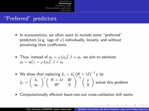
“Preferred” predictors
I In econometrics, we often want to include some “preferred”predictors (e.g. lags of y) individually, linearly, and withoutpenalizing their coefficients
I Thus, instead of yt = ϕ (xt)′β + ut , we aim to estimate
yt = w ′tγ + ϕ (xt)′β + ut
I We show that replacing y∗ = k ′∗ (K + λI )−1 y by
y∗ =
(k∗w∗
)′(K + λI W
W ′ 0
)−1(y0
)solves this problem
I Computationally efficient leave-one-out cross-validation still works
Peter Exterkate (CREATES, Aarhus University) Nonlinear Forecasting with Many Predictors using Kernel Ridge Regression

IntroductionMethodology
Simulation studyMacroeconomic application
Conclusions
“Preferred” predictors
I In econometrics, we often want to include some “preferred”predictors (e.g. lags of y) individually, linearly, and withoutpenalizing their coefficients
I Thus, instead of yt = ϕ (xt)′β + ut , we aim to estimate
yt = w ′tγ + ϕ (xt)′β + ut
I We show that replacing y∗ = k ′∗ (K + λI )−1 y by
y∗ =
(k∗w∗
)′(K + λI W
W ′ 0
)−1(y0
)solves this problem
I Computationally efficient leave-one-out cross-validation still works
Peter Exterkate (CREATES, Aarhus University) Nonlinear Forecasting with Many Predictors using Kernel Ridge Regression

IntroductionMethodology
Simulation studyMacroeconomic application
Conclusions
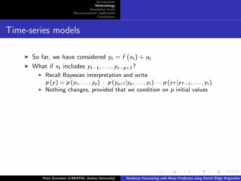
Time-series models
I So far, we have considered yt = f (xt) + ut
I What if xt includes yt−1, . . . , yt−p+1?
I Recall Bayesian interpretation and writep (y) = p (y1, . . . , yp) · p (yp+1|yp, . . . , y1) · · · p (yT |yT−1, . . . , y1)
I Nothing changes, provided that we condition on p initial valuesI Even stationarity does not seem to be an issue
I What if yt is multivariate?
I No problem whatsoever, whether or not Et−1[utu′t ] is diagonal
I So, we could treat e.g. nonlinear VAR-like models
I What if Et−1[u2t
](or Et−1[utu
′t ]) depends on yt−1, . . . , yt−p+1?
I Does not seem analytically tractableI Work in progress, using an iterative approach to estimate mean and
log-volatility equations
Peter Exterkate (CREATES, Aarhus University) Nonlinear Forecasting with Many Predictors using Kernel Ridge Regression

IntroductionMethodology
Simulation studyMacroeconomic application
Conclusions
Time-series models
I So far, we have considered yt = f (xt) + ut
I What if xt includes yt−1, . . . , yt−p+1?I Recall Bayesian interpretation and write
p (y) = p (y1, . . . , yp) · p (yp+1|yp, . . . , y1) · · · p (yT |yT−1, . . . , y1)
I Nothing changes, provided that we condition on p initial valuesI Even stationarity does not seem to be an issue
I What if yt is multivariate?
I No problem whatsoever, whether or not Et−1[utu′t ] is diagonal
I So, we could treat e.g. nonlinear VAR-like models
I What if Et−1[u2t
](or Et−1[utu
′t ]) depends on yt−1, . . . , yt−p+1?
I Does not seem analytically tractableI Work in progress, using an iterative approach to estimate mean and
log-volatility equations
Peter Exterkate (CREATES, Aarhus University) Nonlinear Forecasting with Many Predictors using Kernel Ridge Regression
IntroductionMethodology
Simulation studyMacroeconomic application
Conclusions
Time-series models
I So far, we have considered yt = f (xt) + ut
I What if xt includes yt−1, . . . , yt−p+1?I Recall Bayesian interpretation and write
p (y) = p (y1, . . . , yp) · p (yp+1|yp, . . . , y1) · · · p (yT |yT−1, . . . , y1)I Nothing changes, provided that we condition on p initial values
I Even stationarity does not seem to be an issue
I What if yt is multivariate?
I No problem whatsoever, whether or not Et−1[utu′t ] is diagonal
I So, we could treat e.g. nonlinear VAR-like models
I What if Et−1[u2t
](or Et−1[utu
′t ]) depends on yt−1, . . . , yt−p+1?
I Does not seem analytically tractableI Work in progress, using an iterative approach to estimate mean and
log-volatility equations
Peter Exterkate (CREATES, Aarhus University) Nonlinear Forecasting with Many Predictors using Kernel Ridge Regression

IntroductionMethodology
Simulation studyMacroeconomic application
Conclusions
Time-series models
I So far, we have considered yt = f (xt) + ut
I What if xt includes yt−1, . . . , yt−p+1?I Recall Bayesian interpretation and write
p (y) = p (y1, . . . , yp) · p (yp+1|yp, . . . , y1) · · · p (yT |yT−1, . . . , y1)I Nothing changes, provided that we condition on p initial valuesI Even stationarity does not seem to be an issue
I What if yt is multivariate?I No problem whatsoever, whether or not Et−1[utu
′t ] is diagonal
I So, we could treat e.g. nonlinear VAR-like models
I What if Et−1[u2t
](or Et−1[utu
′t ]) depends on yt−1, . . . , yt−p+1?
I Does not seem analytically tractableI Work in progress, using an iterative approach to estimate mean and
log-volatility equations
Peter Exterkate (CREATES, Aarhus University) Nonlinear Forecasting with Many Predictors using Kernel Ridge Regression

IntroductionMethodology
Simulation studyMacroeconomic application
Conclusions
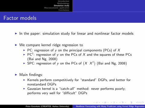
Factor models
I In the paper: simulation study for linear and nonlinear factor models
I We compare kernel ridge regression to
I PC: regression of y on the principal components (PCs) of XI PC2: regression of y on the PCs of X and the squares of these PCs
(Bai and Ng, 2008)I SPC: regression of y on the PCs of
(X X 2
)(Bai and Ng, 2008)
I Main findings:
I Kernels perform competitively for “standard” DGPs, and better fornonstandard DGPs
I Gaussian kernel is a “catch-all” method: never performs poorly;performs very well for “difficult” DGPs
Peter Exterkate (CREATES, Aarhus University) Nonlinear Forecasting with Many Predictors using Kernel Ridge Regression

IntroductionMethodology
Simulation studyMacroeconomic application
Conclusions
Factor models
I In the paper: simulation study for linear and nonlinear factor models
I We compare kernel ridge regression toI PC: regression of y on the principal components (PCs) of XI PC2: regression of y on the PCs of X and the squares of these PCs
(Bai and Ng, 2008)I SPC: regression of y on the PCs of
(X X 2
)(Bai and Ng, 2008)
I Main findings:
I Kernels perform competitively for “standard” DGPs, and better fornonstandard DGPs
I Gaussian kernel is a “catch-all” method: never performs poorly;performs very well for “difficult” DGPs
Peter Exterkate (CREATES, Aarhus University) Nonlinear Forecasting with Many Predictors using Kernel Ridge Regression
IntroductionMethodology
Simulation studyMacroeconomic application
Conclusions
Factor models
I In the paper: simulation study for linear and nonlinear factor models
I We compare kernel ridge regression toI PC: regression of y on the principal components (PCs) of XI PC2: regression of y on the PCs of X and the squares of these PCs
(Bai and Ng, 2008)I SPC: regression of y on the PCs of
(X X 2
)(Bai and Ng, 2008)
I Main findings:I Kernels perform competitively for “standard” DGPs, and better for
nonstandard DGPsI Gaussian kernel is a “catch-all” method: never performs poorly;
performs very well for “difficult” DGPs
Peter Exterkate (CREATES, Aarhus University) Nonlinear Forecasting with Many Predictors using Kernel Ridge Regression

IntroductionMethodology
Simulation studyMacroeconomic application
Conclusions
Other cross-sectional models
I In the companion paper: simulation study for wide range of models,to study the effects of choosing “wrong” kernel or tuning parameters
I Main findings:
I Rules of thumb for selecting tuning parameters work wellI Gaussian kernel acts as a “catch-all” method again, moreso than
polynomial kernels
Peter Exterkate (CREATES, Aarhus University) Nonlinear Forecasting with Many Predictors using Kernel Ridge Regression

IntroductionMethodology
Simulation studyMacroeconomic application
Conclusions
Other cross-sectional models
I In the companion paper: simulation study for wide range of models,to study the effects of choosing “wrong” kernel or tuning parameters
I Main findings:I Rules of thumb for selecting tuning parameters work wellI Gaussian kernel acts as a “catch-all” method again, moreso than
polynomial kernels
Peter Exterkate (CREATES, Aarhus University) Nonlinear Forecasting with Many Predictors using Kernel Ridge Regression

IntroductionMethodology
Simulation studyMacroeconomic application
Conclusions
Data
I 132 U.S. macroeconomic variables, 1959:1-2010:1, monthlyobservations, transformed to stationarity (Stock and Watson, 2002)
I We forecast four key series: Industrial Production, Personal Income,Manufacturing & Trade Sales, and Employment
I h-month-ahead out-of-sample forecasts of annualized h-monthgrowth rate yh
t+h = 1200h ln (yt+h/yt), for h = 1, 3, 6, 12
I Rolling estimation window of length 120 months
Peter Exterkate (CREATES, Aarhus University) Nonlinear Forecasting with Many Predictors using Kernel Ridge Regression

IntroductionMethodology
Simulation studyMacroeconomic application
Conclusions
Competing models
I Standard benchmarks: mean, random walk, AR
I DI-AR-Lag framework (Stock and Watson, 2002): regressors arelagged yt and lagged factors
I Factors extracted using PC, PC2, or SPCI Lag lengths and number of factors reselected for each forecast by
minimizing BIC
I Kernel ridge regression: same setup, but with lagged factorsreplaced by ϕ (lagged xt)
I Polynomial kernels of degree 1 and 2, and the Gaussian kernelI Lag lengths, λ and σ selected by leave-one-out cross-validation
Peter Exterkate (CREATES, Aarhus University) Nonlinear Forecasting with Many Predictors using Kernel Ridge Regression
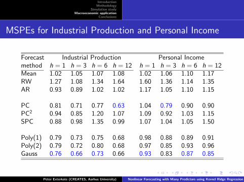
IntroductionMethodology
Simulation studyMacroeconomic application
Conclusions
MSPEs for Industrial Production and Personal Income
Forecast Industrial Production Personal Incomemethod h = 1 h = 3 h = 6 h = 12 h = 1 h = 3 h = 6 h = 12Mean 1.02 1.05 1.07 1.08 1.02 1.06 1.10 1.17RW 1.27 1.08 1.34 1.64 1.60 1.36 1.14 1.35AR 0.93 0.89 1.02 1.02 1.17 1.05 1.10 1.15
PC 0.81 0.71 0.77 0.63 1.04 0.79 0.90 0.90PC2 0.94 0.85 1.20 1.07 1.09 0.92 1.03 1.15SPC 0.88 0.98 1.35 0.99 1.07 1.04 1.05 1.50
Poly(1) 0.79 0.73 0.75 0.68 0.98 0.88 0.89 0.91Poly(2) 0.79 0.72 0.80 0.68 0.97 0.85 0.93 0.96Gauss 0.76 0.66 0.73 0.66 0.93 0.83 0.87 0.85
Peter Exterkate (CREATES, Aarhus University) Nonlinear Forecasting with Many Predictors using Kernel Ridge Regression

IntroductionMethodology
Simulation studyMacroeconomic application
Conclusions
MSPEs for Industrial Production and Personal Income
I Simple PC performs better than its nonlinear extensions
I Kernel methods perform even slightly better
I “Infinite-dimensional”, smooth Gaussian kernel is a safe choice
I Good results at all horizons
Peter Exterkate (CREATES, Aarhus University) Nonlinear Forecasting with Many Predictors using Kernel Ridge Regression

IntroductionMethodology
Simulation studyMacroeconomic application
Conclusions
MSPEs for Manufacturing & Trade Sales and Employment
Forecast Manufacturing & Trade Sales Employmentmethod h = 1 h = 3 h = 6 h = 12 h = 1 h = 3 h = 6 h = 12Mean 1.01 1.03 1.05 1.08 0.98 0.96 0.97 0.97RW 2.17 1.49 1.45 1.53 1.68 0.95 1.00 1.20AR 1.01 1.02 1.10 1.08 0.96 0.85 0.90 0.96
PC 0.89 0.80 0.77 0.63 0.76 0.56 0.48 0.48PC2 0.94 0.97 1.13 1.06 0.76 0.61 0.69 0.60SPC 0.99 1.18 1.59 1.02 0.81 0.81 0.90 0.72
Poly(1) 0.94 0.88 0.78 0.64 0.90 0.69 0.65 0.55Poly(2) 0.96 0.88 0.81 0.67 0.95 0.70 0.69 0.64Gauss 0.94 0.87 0.80 0.64 0.88 0.68 0.64 0.59
Peter Exterkate (CREATES, Aarhus University) Nonlinear Forecasting with Many Predictors using Kernel Ridge Regression
IntroductionMethodology
Simulation studyMacroeconomic application
Conclusions
MSPEs for Manufacturing & Trade Sales and Employment
I Small losses at all horizons
I Linear model is apparently sufficient here, but Gaussian KRRcontinues to yield adequate results
I Both PC and KRR work very well
I PC outperforms all other methods
Peter Exterkate (CREATES, Aarhus University) Nonlinear Forecasting with Many Predictors using Kernel Ridge Regression

IntroductionMethodology
Simulation studyMacroeconomic application
Conclusions
A closer look at performance
I So, KRR performs worse than PC only if PC performs very well
I To see if this result also holds over time, we computed mean squaredprediction errors for each ten-year window separately
I All methods yield larger errors in more volatile periods
I However: smaller relative errors in more volatile periods
I KRR produces more volatile relative errors than PC⇒ KRR most valuable in turmoil periods, including 2008-9 crisis
Peter Exterkate (CREATES, Aarhus University) Nonlinear Forecasting with Many Predictors using Kernel Ridge Regression

IntroductionMethodology
Simulation studyMacroeconomic application
Conclusions
Forecast encompassing regressions
I Forecast encompassing regression:
yht+h = α yh, PC or KRR
t+h|t + (1− α) yh, ARt+h|t + uh
t+h
I Hypotheses of interest: α = 0 and α = 1
I Across all series and horizons, α = 0 is strongly rejected for PC andfor all KRR forecasts
I In many cases, α = 1 cannot be rejected
I Thus, PC and KRR forecasts encompass AR forecasts
Peter Exterkate (CREATES, Aarhus University) Nonlinear Forecasting with Many Predictors using Kernel Ridge Regression
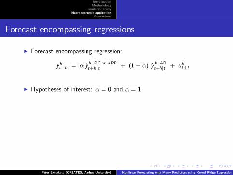
IntroductionMethodology
Simulation studyMacroeconomic application
Conclusions
Forecast encompassing regressions
I Forecast encompassing regression:
yht+h = α yh, PC or KRR
t+h|t + (1− α) yh, ARt+h|t + uh
t+h
I Hypotheses of interest: α = 0 and α = 1
I Across all series and horizons, α = 0 is strongly rejected for PC andfor all KRR forecasts
I In many cases, α = 1 cannot be rejected
I Thus, PC and KRR forecasts encompass AR forecasts
Peter Exterkate (CREATES, Aarhus University) Nonlinear Forecasting with Many Predictors using Kernel Ridge Regression
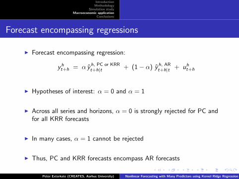
IntroductionMethodology
Simulation studyMacroeconomic application
Conclusions
Forecast encompassing regressions
I Forecast encompassing regression:
yht+h = α yh, PC or KRR
t+h|t + (1− α) yh, ARt+h|t + uh
t+h
I Hypotheses of interest: α = 0 and α = 1
I Across all series and horizons, α = 0 is strongly rejected for PC andfor all KRR forecasts
I In many cases, α = 1 cannot be rejected
I Thus, PC and KRR forecasts encompass AR forecasts
Peter Exterkate (CREATES, Aarhus University) Nonlinear Forecasting with Many Predictors using Kernel Ridge Regression

IntroductionMethodology
Simulation studyMacroeconomic application
Conclusions
Forecast encompassing regressions
I Also compare kernels and PC:
yht+h = α yh, KRR
t+h|t + (1− α) yh, PCt+h|t + uh
t+h
I In most cases, we reject both α = 0 and α = 1
I That is, 0 < α < 1: KRR and PC forecasts are complements
Peter Exterkate (CREATES, Aarhus University) Nonlinear Forecasting with Many Predictors using Kernel Ridge Regression

IntroductionMethodology
Simulation studyMacroeconomic application
Conclusions
Conclusions
I Kernel ridge regression provides a natural way of dealing withhigh-dimensionality and nonlinearity
I It can also handle time-series models with constant conditionalvolatilities and correlations, even if they are nonstationary
I Selection of kernel and tuning parameters can be fully automated:easy-to-use black-box implementation for nonlinear forecasting
I Macro forecasting: KRR outperforms more traditional methods
I Best forecast performance in turmoil periods
I The “smooth” Gaussian kernel generally performs best
Peter Exterkate (CREATES, Aarhus University) Nonlinear Forecasting with Many Predictors using Kernel Ridge Regression

IntroductionMethodology
Simulation studyMacroeconomic application
Conclusions
Current research
I Examine a wider range of kernel functions
I So far, Gaussian kernel holds up very well
I Extend the methodology to models with time-varying volatility
I This will enable applications to financial data
Peter Exterkate (CREATES, Aarhus University) Nonlinear Forecasting with Many Predictors using Kernel Ridge Regression

IntroductionMethodology
Simulation studyMacroeconomic application
Conclusions
Current research
I Examine a wider range of kernel functionsI So far, Gaussian kernel holds up very well
I Extend the methodology to models with time-varying volatilityI This will enable applications to financial data
Peter Exterkate (CREATES, Aarhus University) Nonlinear Forecasting with Many Predictors using Kernel Ridge Regression