Embed Size (px)
Citation preview
Limited Arbitrage and Pricing Discrepancies in Credit Markets
Kasing Man, Junbo Wang, and Chunchi Wu*
November 10, 2013
Abstract
In this paper we investigate the roles of nondefault risk factors and impediments to arbitrage in
the pricing discrepancies of credit markets. We find that nondefault factors contribute to the
unusual price distortions in credit markets and the noise in CDS price signals during the crisis.
However, there is ample evidence that impediments to arbitrage play a more important role in
turbulent markets. Impediments to arbitrage result in less market integration and more persistent
pricing discrepancies. These effects are more severe for riskier and less liquid firms and in times
of stress.
JEL classification: G01; G12
Keywords: impediments to arbitrage; pricing discrepancies; default and nondefault risk factors;
slow moving capital; search frictions; long memory; cointegration; price discovery
* Kasing Man is at Western Illinois University, Junbo Wang is at City University of Hong Kong, and Chunchi Wu is
at State University of New York at Buffalo.
2
1. Introduction
The arbitrage-free condition has been a building block in development of modern asset
pricing theories. This condition however was severely violated during the subprime crisis in
various markets (see Duffie, 2010; Mitchell and Pulvino, 2012; Kapadia and Pu, 2012).1
Particularly the dramatic violations of the arbitrage-based pricing relationship in credit risk
markets during the crisis have attracted a lot of attention. The credit default swap (CDS) spread
is normally within a small difference from the yield spread of a reference par bond with the same
maturity as the CDS. This spread difference (basis) however widened to above 600 basis points
for speculative-grade bonds shortly after the collapse of Lehman Brothers in 2009. As Duffie
points out in his 2010 American Finance Association presidential address, “The extreme
negative CDS basis ‘violations’ … across broad portfolios of investment-grade bonds and high-
yield bonds, respectively, is far too large to be realistically explained by CDS counterparty risk
or by other minor technical details.”
What might have caused the large pricing discrepancy in credit markets? One possibility is
that markets may price different factors for two related assets. If so, pricing discrepancies are not
a real anomaly. Instead, it could be due to a misspecification of risk factors in the credit
valuation model. For instance, illiquidity can be an important pricing factor for the corporate
bond but not for the CDS. So, when there is an aggregate illiquidity shock, corporate bonds
experience a price discount or yield jump, leading to a negative CDS basis. Likewise,
counterparty credit risk is perceived to be a more important factor for the credit derivatives
market. Heightened counterparty credit risk for CDS sellers will make the CDS worth less and
hence have a negative impact on the basis.
Another possibility for pricing discrepancies is limits to arbitrage. Significant impediments to
1 For example, there were serious violations of covered interest rate parity, a negative spread between Treasury bond
yields and LIBOR swap rates, and a breakdown of the capital structure arbitrage across equity and credit markets.
3
arbitrage can cause large and persistent pricing discrepancies between two similar assets. To take
the profitable opportunities when the basis becomes significantly negative, one can short a risk-
free bond, use the proceeds to invest in the corporate bond, and buy a CDS of the bond.2
However, arbitrage is not without costs or constraints. Search costs, market illiquidity and
uncertainty, funding constraints, or slow capital movement can impede the arbitrage. For
example, arbitrageurs may not be able to unwind their positions profitably in the short term when
the market is illiquid. An attempt to arbitrage pricing discrepancies away can also be risky when
the price persistently deviates from its equilibrium value as arbitrageurs typically have short
investment horizons and cannot sustain large losses (Shleifer and Vishny, 1997; Pontiff, 2006;
Gorton and Metrick, 2012). Limited arbitrage of this nature can cause pricing discrepancies to
persist over a sustained period of time.
Understanding the causes for pricing discrepancies in two similar markets is important for
development of general asset pricing theory. The subprime crisis provides an excellent
opportunity to understand the market function and price dynamics in times of stress. A unique
feature of this crisis is the drastic deterioration in liquidity and credit quality in financial markets.
Many large financial institutions incurred substantial portfolio losses and liquidity suddenly
dried up in the midst of the crisis. Failure to regain capital promptly impaired the ability of
financial intermediaries to absorb supply shocks. Several studies have ascribed the unusual price
distortions to this problem (see, for example, Mitchell, Pedersen and Pulvino, 2007; Duffie,
2010; Mitchell and Pulvino, 2012). As explained by these studies, impediments to capital
movement, such as time required to raise capital and inefficiency in search for trading
counterparties, prevent arbitrageurs from exploiting the profitable opportunities and cause
extreme pricing discrepancies.
In this paper, we examine different hypotheses for the pricing discrepancies between the
2 The profit of this strategy is the principal debt position times the absolute magnitude of the basis.

4
CDS and corporate bond and the channels through which this problem occur. In particular, we
investigate the possibility that the CDS and corporate bond markets may price different factors as
well as the role of limits-to-arbitrage in explaining the pricing anomaly in credit markets. In
pursuing these investigations, we address a number of important issues related to the pricing of
CDS and corporate bonds and the relationship between the two markets. Do bond and CDS
spreads contain different nondefault pricing factors which contribute to pricing discrepancies?
Are the CDS and corporate bond markets integrated? If not, is it due to differences in pricing
factors or impediments to arbitrage? Does the CDS market lead the bond market in price
discovery in the short term and provide credible signals for credit risk? Do impediments to
arbitrage lead to more persistent pricing discrepancies between the CDS and corporate bond
markets during the subprime crisis? By addressing these issues, we attempt to shed more light on
the causes of extreme price distortions in credit markets and improve understanding on asset
price dynamics.
We find that nondefault risk factors contribute to the negative CDS basis because bond
spreads are more sensitive to these factors. However, nondefault factors can only explain some
of the pricing discrepancies between the CDS and corporate bond markets. Empirical evidence
suggests that impediments to arbitrage are the fundamental cause for pricing discrepancies and
lack of integration in the CDS and corporate bond markets. Firms with high idiosyncratic risk
and trading cost and low liquidity face greater pricing discrepancies and less market integration.
Pricing discrepancies are more severe for speculative-grade firms and during the subprime crisis.
Both the level and volatility of the basis become more persistent during the crisis period and
exhibit long memory, supporting Duffie’s (2010) hypothesis that impediments to arbitrage cause
persistence in pricing discrepancies over longer horizons.
Our focus on the relationship between the CDS and corporate bond markets is related to
several recent important papers on this issue (Blanco, Brennan, and Marsh, 2005; Duffie, 2010;

5
Nashikkar, Subrahmanyam, and Mahanti, 2011; Bai and Collin-Dufresne, 2013; Das,
Kalimipalli, and Nayak, 2013). Our work differs from these studies in several aspects. First, we
explore the roles of both impediments to arbitrage and differential nondefault pricing factors in
explaining CDS-bond pricing discrepancies. Second, we look into the channels through which
pricing discrepancies may occur. Third, we investigate whether firm-level impediments to
arbitrage can explain the price divergence in the CDS and bond markets. Lastly, we test Duffie’s
(2010) hypothesis of slow capital movement and persistent pricing discrepancies using long
memory time-series models.
The remainder of this paper is organized as follows. Section 2 discusses the research issues
and empirical methodology. Section 3 describes the data and presents empirical results and
Section 4 examines the persistence of pricing discrepancies and volatility in the credit markets.
Finally, Section 5 summarizes our major findings and concludes the paper.
2. Methodology
In this section, we explore pricing factors in the CDS and corporate bond markets and the
relation between these markets, and present methodologies for empirical tests.
2.1 The relation between CDS and bond yield spreads
CDS and bond yield spreads both reflect the default risk of corporate bonds. In addition, the
literature has suggested that these spreads contain nondefault components associated with
liquidity, counterparty risk and bond characteristics. To the extent that the importance of these
factors differs between the two markets, CDS and bond spreads can deviate. Denote the CDS and
bond yield spreads as
c c c c
it it it it it itCDS L F , (1)
b b b
it it it it itBYS L F (2)
where CDSit and BYSit are credit default swap rates and corporate bond yield spreads for entity i
6
at time t, λit is the default premium, j
itL is the liquidity premium, c
it is the counterparty risk
premium, Fj represents effects of other factors such as frictions and aggregate shocks, j
i is the
noise term and the superscript j = c, b denotes the CDS and bond, respectively.
In this specification, CDS and the reference bond spreads share a common default risk
component. In an efficient market, default risk should be priced equally across markets to give
the same default premium λit. Besides default risk, the literature has shown that liquidity is an
important pricing factor in credit markets (see, for example, Bongaerts, de Jong and Driessen,
2011; Lin, Wang, and Wu, 2011; Friewald, Jankowitsch, Subrahmanyam, 2012; Dick-Nielsen,
Feldhutter, and Lando, 2012). However, the magnitude of the liquidity component can differ
between the two securities. For one, the CDS market is more liquid than the corporate bond
market. In addition, sensitivity to liquidity shocks can differ between the two securities. For
counterparty risk, as it is perceived to be more relevant for the derivatives market (Jarrow and
Yu, 2001; Arora, Gandhi and Longstaff, 2012), we add this risk component in the CDS spread.
Finally, j
itF represents other factors such as search frictions, bond characteristics and aggregate
shocks that can affect the pricing of the CDS and corporate bonds.
The basis is the difference between the CDS spread and the bond yield spread (BYS),
it it itBasis CDS BYS (3)
If both CDS and bond spreads contain only the common default component, the no-arbitrage
condition implies a zero basis. Even in this simplified case, the arbitrage can only be perfect if
the spread on a par risky floating-rate bond over a risk-free floating rate bond equals the CDS
spread or if the payment dates on the bond and the CDS are identical (see Duffie, 1999;
Houweling and Vorst, 2005; Hull, Predescu and White, 2004). Cheapest-to-delivery options and
costs of short-selling bonds can also derail the arbitrage-based pricing relationship.
An important issue is whether CDS and bond spreads contain different nondefault
7
components. If one market prices a factor that is not priced in the other market, the basis will by
nature not converge to zero. For instance, if counterparty risk is important for the CDS but is
trivial for the corporate bond, the basis will reflect this risk premium for the CDS. Similarly, if
the liquidity premium component is more important for corporate bonds, it can lead to a negative
basis. Also, firm/bond characteristics and supply/demand shocks can have different effects on
CDS and bond prices. For example, selling pressure and deleveraging by dealer banks is likely to
have a larger impact on the bond price than the CDS rate. Also, bond-specific liquidity
characteristics would be less relevant to the CDS pricing. We can express CDS basis as a
function of these nondefault factors:
( , , ), ,j c j
it it it itBasis f L F j c b (3a)
where the default risk premium is netted out.
In empirical investigation, we examine the roles of nondefault factors in explaining the CDS-
bond pricing discrepancies by running regressions of the basis, CDS spreads and bond spreads,
respectively, against these factors. The sensitivity of CDS and bond spreads to each factor
provides important information for the sources of pricing discrepancies and the relative
contribution of each factor to the negative CDS spread. For example, if bond spreads are more
sensitive to illiquidity and supply shocks than CDS spreads do, then the greater effects of these
risk factors on bonds contribute to the negative CDS spread. The coefficients in the spread and
basis regressions allow us to infer the role of each nondefault factor in affecting the CDS basis.
2.2. Market integration and price discovery
2.2.1. Cointegration tests
If default is the only risk factor for the CDS and corporate bond, the two markets should be
integrated under rationality. When there are nondefault factors, the cointegration hypothesis can
be rejected for two reasons. First, the CDS and corporate bond markets price different factors.

8
Pricing discrepancies are therefore not real anomalies if the CDS and bond prices are evaluated
against the true credit pricing model. Second, there are impediments to arbitrage. If so, the
cointegration hypothesis can still be rejected even if we account for the effects of nondefault risk
factors on the CDS and bond prices using the correct valuation model.
To examine whether the CDS and corporate bond markets are cointegrated, we perform two
tests: one is based on the observed (raw) spreads and the other based on the spreads adjusted for
the nondefault components. These tests allow us to assess the role of nondefault factors in the
long-term relation between the two markets. The adjusted spreads are the CDS and bond spreads
adjusted for the effects of nondefault factors. These adjusted CDS and bond spreads can be
viewed as pure default spreads, which should be equal if the market is integrated. If nondefault
risk factors are the reason for rejecting the hypothesis, the two series of adjusted spreads should
be cointegrated. Otherwise, limits-to-arbitrage is likely to be the cause for violation of market
integration.
To perform the cointegration test, we estimate the vector error-correction model (VECM) of
CDS and bond spreads. Denote )',( ttt qpY , where tp and tq are CDS and bond spreads,
respectively, unadjusted or adjusted for nondefault components. The VECM model can be
written as
t
r
i
ititt eYYbcY
1
1
1' , (4)
where c is the constant term, et’s are serially uncorrelated innovations with mean zero and
covariance matrix )( teVar with diagonal elements 2
1 and 2
2 and off-diagonal elements 21 ,
)',1( b is the cointegration vector with the first element normalized to one, )',( 21 is
the vector of responses for the error-correction term, and B 1 is the difference operator with
B being the back-shift operator. We apply Johansen's trace test to the VECM to determine the
number of cointegrated vectors. Details of this test procedure are described in Appendix A.

9
Blanco, Brennan, and Marsh (2005) examine the long-run equilibrium relation between the
CDS and corporate bond markets using the pre-crisis data. By contrast, we examine the relations
between the two markets in the normal and crisis periods. More importantly, we investigate
whether the rejection of the cointegration hypothesis is due to nondefault risk factors or
impediments to the arbitrage.
2.2.2 Nonparametric tests
Besides the cointegration test, we carry out a nonparametric test for market integration.3
When the CDS basis is significantly negative, the bond spread should move down and the CDS
spread should move up to close the gap if markets are integrated. If instead the CDS and bond
spreads move in the same direction, a pair of CDS and bond prices can remain divergent and
present an arbitrage opportunity. Thus, we can perform a nonparametric test for market
integration based on the frequency of observations for such arbitrage opportunities. For a given
period with k = 1, 2,…,T observations, we define γi for firm i as
, ,
1
[ 0]1 1
1i k i k
T T
i CDS BYSk
(5)
where , ( ) ( )i k i iCDS CDS k CDS k and
, ( ) ( )i k i iBYS BYS k BYS k , k ≤ T - τ, 1 ≤ τ ≤
T – 1, τ indicates a non-overlapping time interval and T is the number of observations. For a
given T, firm i’s bond and CDS markets are more integrated than those of firm j, if γi < γj. γ is
related to the Kendall correlation κ in that 4
1( 1)T T
. In the absence of mispricing, κ = -1.
More generally, a larger κ corresponds to less integrated markets.
There are advantages for this nonparametric test on market integration. First, the
nonparametric measure is not model-dependent and is thus robust to potential nonlinearities in
the CDS and bond spread relation. Additionally, the measure accounts for all possible pairs from
3 Bakshi, Cao and Chen (2000) use a similar approach to study the relation between the stock and option markets.

10
T observations and is independent of the horizon over which spreads are observed. For
robustness, we compare the result of this test with the time-series test for market cointegration.
2.3 Price discovery
Even if credit risk prices in CDS and bond markets converge to a common efficient price in
the long run, they can deviate from each other in the short run due to different speeds of
adjusting to new information or frictions. From the microstructure point of view, it is important
to evaluate the information content of prices and to know which market provides more timely
information for credit risk. When similar securities are traded in a single centralized market,
price discovery is solely produced by that market. Conversely, when trades of similar securities
take place in multiple trading venues, questions naturally arise as to what is the relative
contribution of each venue to price discovery of the whole market. The CDS market is perceived
to be more liquid than the corporate bond market. If the information is impounded in a liquid
market faster, credit risk prices in the CDS market will lead prices in the corporate bond market
and the former will assume the price leadership.
We employ two price discovery measures suggested by Hasbrouck (1995) and Gonzalo-
Granger (1995) to assess the price leadership in the credit risk market. These are standard price
discovery measures in market microstructure literature. In brief, the Gonzalo-Granger method
decomposes the price into permanent and transitory components, and associates the permanent
component with the long run price. This price discovery measure depends on the speed of
adjustment of the preceding disequilibrium in prices in the two markets. By contrast, the
Hasbrouck price discovery measure takes into consideration the innovations in the two markets.
The parameters estimated from the VECM in (4) can be used to construct the price discovery
measures. The Gonzalo-Granger (G) measure for tp and tq are defined as
21
21
G , and
21
12
G . (6)

11
By construction, the G measure is based on the speed ( ) of the error-correction term, or how
price in each market changes in response to the price disequilibrium in the preceding period.
Hasbrouck’s information share (S) measures are defined as
,)1()(
)()(
22
21
2
2112
2
21121
uS
2 2
1 2
22 2 2
2 1 1 2 1 2
( 1 )( ) ,
( ) ( 1 )S l
(7)
where u indicates the upper bound and l is the lower bound. In addition to the speed of
adjustment, Hasbrouck’s information share measure incorporates the innovations of the two
markets through their covariance structure.
Note that Hasbrouck’s measures depend on the ordering of the price series. For )',( ttt qpY ,
the measures above give the upper bound (maximum) for the first price series tp and the lower
bound (minimum) for the second price series tq . Reversing the order in the vector of the price
series )',( tt pq gives the upper bound )(2 uS for tq and the lower bound )(1 lS for tp . For small
correlation between innovations in the two markets, the upper and lower bounds will be close.
In practice, the average of the two bounds is used as a summary measure of information share.
We use these price discovery measures to assess the price leadership role of the CDS and
corporate bond markets in the pre-crisis and the subprime crisis periods. This analysis focuses on
the dynamic behavior of CDS and bond yield spreads with lead-lag relations. It contrasts the
cointegration test which deals with the long-run equilibrium relation between the two markets.
2.4 Persistence in pricing discrepancies and volatility
Duffie (2010) argues that slow movement in investment capital to trading opportunities is a
fundamental cause for the unusual negative basis during the subprime crisis. His model suggests
that slow capital movement leads to persistent pricing discrepancies. The slower the movement
12
in investment capital or the longer it takes for financial intermediaries to regain capital, the lower
is the supply of capital to support arbitrage trading and therefore, the more persistent will be the
pricing discrepancies between the CDS and bond spreads. We test this hypothesis based on the
level and changes in the CDS basis.
2.4.1. Time-series tests for the persistence of pricing discrepancies
We employ two approaches to study price persistence. The first one is the impulse response
analysis. The impulse response analysis provides a direct diagnosis for price persistence after an
exogenous shock, which can be easily visualized. The second approach involves estimating
persistence or a long memory parameter commonly used in the literature of financial time-series.
We use the impulse response function (IRF) to examine the speed and dynamic responses of
the CDS and bond spreads to an external shock (see Appendix B for the detail of the estimation
procedure). If capital movement is slow, it will take longer time for the spreads of the CDS and
reference bond to converge after an exogenous shock. Also, the initial impact of the shock on
spreads will be stronger in a less liquid market. Thus, we can compare the results in the normal
period and in the crisis period with slow capital movement to see if there are significant
differences in impulse responses.
In addition, we can measure the persistence of the pricing discrepancy between the CDS and
bond prices using time-series models. Persistence behavior of the CDS basis can be best studied
through the long-range dependency or long memory. Using this approach, we study pricing
discrepancy persistence by estimating the long memory parameter d. For a price series with long
memory, the autocorrelation between two observations k period apart decays in a slower
hyperbolic rate of 12 dk as opposed to the faster exponential rate of ka for a short memory time
series. A persistent time series does not have summable autocorrelations, and it is the slow

13
declining rate of autocorrelations that generates the persistence behavior.4
There are a number of ways to estimate the long memory parameter d. Here we employ the
rescaled range R/S method which is widely used in the literature. The R/S statistic is originally
proposed by Hurst (1951) and modified by Lo (1991). The R/S statistic is defined as
][1
mMs
QN
N (8)
where
k
j
jNk yyM1
1 )(max is the cumulative maximum,
k
j
jNk yym1
1 )(min is the
cumulative minimum,
N
j
jN yyN
s1
2 )(1
is the sample variance, and N is the sample size.
Intuitively, consider a series of gains or losses of an investment over a period of time of
length N. Within the period, M is the highest net cumulative gain, while m is the lowest net
position. If there are persistent gains or losses (i.e., the series tends to be consistently above or
below the mean over a sustained period), the cumulative max M minus cumulative min m will
tend to be large. On the other hand, if there are short gains or losses (i.e., the series tends to move
above and below the mean quickly), then M minus m would tend to be small. Thus, a larger R/S
statistic suggests a persistent behavior. In essence, R/S is simply a suitably adjusted range
statistic,5 where the range is the difference between the cumulative high and low positions.
The range scaled by the standard deviation will converge to a random variable at the rate of
5.0N if there is no long memory, and at a faster rate 5.0dN if there is long memory. Thus, the
4Consider a simple long memory time series model (1 )d
t tB x e where B is the back-shift operator, te is a
stationary ARMA process and x in the time series, where d is a real number between -0.5 and 0.5. This fractional
difference series exhibits persistent behavior can be seen as follows. Taking a binomial expansion of (1 )d
tB x
gives: 0
j t j tj
b x e
where 10 b and ( )
( ) ( 1)j
j db
d j
is the binomial coefficient, and 1
( )
d
j
jb
d
for large j.
Thus, the model can be considered as an AR model of an infinite order with slow decaying coefficients. Such
dependency of the series on its infinite past is the basis for its persistence behavior. Furthermore, it can be shown
that the lag k autocorrelation of tx decays in an hyperbolic rate, )( 12 d
k kO , and that the autocorrelations are
not summable (see Hosking, 1981). For a time series which follows a fractionally integrated ARFIMA (p, d, q)
model, the time series is stationary when d is between -0.5 and 0.5. 5 Lo’s (1991) modified R/S statistic replaces the standard deviation by the square root of Newey-West estimate of
the long-run variance.

14
slope in the log-log plot of R/S statistic versus N gives the Hurst parameter H = d + 0.5.6 We use
the R/S statistic to measure persistence in the CDS basis in the normal and crisis periods. A
higher d estimate signifies a more persistent behavior that a higher basis level tends to
accompany with another higher level, and low by low.
2.4.2. Tests of volatility persistence
Similarly, we can test whether the change of the pricing discrepancy or volatility is
persistent. If there is slow capital movement or significant impediments to arbitrage, changes in
the CDS basis will be more persistent. A simple way to capture this phenomenon is by the
absolute daily basis change and for this we can study the persistence behavior using the R/S
statistic discussed above. But a more formal way is to analyze volatility persistence in the
GARCH setting as basis changes exhibit pronounced volatility clustering. This approach studies
volatility persistence within the GARCH framework.
We employ a long memory GARCH model called the frictionally integrated GARCH model
(FIGARCH) proposed by Baillie, Bollerslev and Mikkelsen (1996) to measure volatility
persistence through the long memory parameter d. Consider an MA(1)-GARCH(1,1) model for
the basis change:
11 ttt eecbasis (9)
2
11
2
110
2
ttt e (10)
where the conditional variance of the error term te is 2
t . Let 22
ttt ev ; then we can rewrite
the conditional variance equation as
tt vBeB )1(])(1[ 10
2
11
where B is the back-shift operator. The FIGARCH model introduces a long memory parameter d
into the squared residuals equation:
6 For details, see Zivot and Wang (2006, chapter 8).
15
tt
d vBeBB )1()1]()(1[ 10
2
11 (11)
or,
2
0
2 ])1)(()([)( t
d
t BBBB (12)
where BB )(1)( 11 and BB 11)( . The parameter d captures the persistence
behavior of volatility. Baillie et al (1996) show that the model is strictly stationary when d is
between 0 and 1.7 We perform the persistence tests using daily CDS basis data.
3. Data and empirical results
3.1. Data
Our sample includes data from the CDS, bond and stock markets. Daily credit default swap
(CDS) data are provided by the Markit Group. Bond transaction data are from the Trade
Reporting and Compliance Engine (TRACE), and bond characteristic information is from the
Fixed Investment Securities Database (FISD). Daily stock returns are from the Center for
Research in Security Prices (CRSP). To compare the behavior of the CDS basis before and after
the onset of the subprime crisis, we set our sample period from January 2005 to December 2009.
CDSs are over-the-counter derivatives, and their rates are quoted typically in basis points.
Markit Group constructs the daily composite CDS spread by aggregating dealer quotes. For each
reference entity, a large number of CDS contracts can exist with differences in maturity,
currency denomination, seniority of reference bonds, and treatment of restructuring in credit
event definition. We choose the US dollar-denominated 5-year CDS contracts on senior
unsecured debts with modified restructuring (MR). Also, because of the need to match CDS data
with other databases, we focus on the US reference entities.
TRACE provides prices, yields, par value of a transaction and other trading information of
corporate bonds. The FISD database contains issue- and issuer-specific information, such as
7 Note that this is unlike the stationary region of -0.5 and 0.5 for an ARFIMA model.

16
coupon rate and frequency, maturity date, issue amount, provisions and credit rating history, for
all US corporate bonds maturing in 1990 or later.
We match the 5-year CDS contract with reference bonds of the same maturity. We obtain the
yield of the 5-year bond from a set of bonds with maturities that bracket the 5-year horizon. For
each reference entity, we search TRACE for a set of bonds with 3 to 5 years left to maturity, and
another set of bonds with maturity longer than 6 years at the start of each year. By regressing the
yields of these bonds against maturities, we obtain the yield to maturity for a five-year bond to
match the CDS. To calculate yield spreads of bonds, we use the five-year swap rate as the
reference rate. Swap rates are collected from the Federal Reserve Board.
We use several variables related to counterparty risk, liquidity, market uncertainty and
aggregate shocks to explain the CDS basis behavior. We use the Libor-OIS spread (LOIS) as a
counterparty risk measure, which is the difference between the 3-month Libor rate and the
overnight index swap rate. This spread has been shown to be an effective measure of
counterparty credit risk of financial intermediaries (see Gorton and Metrick, 2012). Libor and
OIS are from Bloomberg. In addition, we use average CDS rates for primary dealers to measure
the credit risk of market makers.
We consider broad liquidity measures to capture the effect of illiquidity in financial markets.
These include Amihud and Pastor-Stambaugh bond and stock market liquidity measures, on/off-
the-run spreads, money market fund flow (MMFF) and the liquidity factor constructed by Hu,
Pan and Wang (2012) from the Treasury market. The Pastor-Stambaugh stock market liquidity
index is downloaded from WRDS. The Pastor-Stambaugh bond market liquidity index is
constructed using the same method as in Pastor and Stambaugh (2003). The Amihud stock and
bond market liquidity indices are constructed using the procedure suggested by Amihud (2002).8
8 The Amihud illiquidity measures are scaled by the ratio of capitalizations of stocks and bonds to obtain the
innovations using a procedure similar to Lin et al. (2011).
17
The data for money market fund flow and on-the-run bond yield are from Bloomberg and off-
the-run bond yields are from the Federal Reserve Board (see Gurkaynak, Sack, and Wright,
2007). Moreover, we use liquidity characteristics such as the amount of issuance and age as
proxies for bond-specific illiquidity. The age variable is the average age of bonds that we use to
construct the 5-year bond yield. Additionally, we use the CDS bid-ask spreads as a proxy for
liquidity. Bond liquidity characteristics are obtained from the FISD and CDS bid-ask spreads are
from Bloomberg.
Aggregate supply or demand shocks can cause deleveraging and market uncertainty. We use
VIX (volatility index) provided by the Chicago Board Options Exchange (CBOE) as a proxy for
market uncertainty. To capture the effect of selling and pricing pressure, we calculate the change
in the primary dealer position in long-term corporate securities and use it as a measure of
deleveraging. The data are obtained from the Federal Reserve Bank of New York.
We keep only the reference entities for which CDS, stock and bond data are available over
the sample period. Our sample includes 138,518 daily observations for 453 firm/year reference
entities from 198 firms. The data sample includes firms from 11 industries and the sample size is
much larger than that employed by Blanco et al. (2005) and Longstaff et al. (2005).
Table 1 provides a summary of the data sample. Over the whole sample period, average basis
is negative (-.35%), which is largely due to the reverse relation between CDS and bond spreads
during the financial crisis. We use July 1, 2007 as the cutoff for the normal and crisis periods
(see also Friewald et al., 2012; Dick-Nielsen et al., 2012). During the normal period (January
2005 to June 2007), average basis is slightly positive. It then becomes quite negative (-.82%)
during the crisis period (July 2007 to December 2009). Much of this reversion is because bond
spreads increase more rapidly than CDS rates during the financial crisis. Volatility of the basis
also increases considerably during the crisis period, about 10 times of the magnitude during the
normal period. Bond volatility is higher than CDS volatility. Both yield spreads and CDS rates
18
become much more volatile during the crisis with the volatility of the former being higher than
the latter.
[Insert Table 1 Here]
The patterns of the negative basis and high volatility are more pronounced for speculative-
grade bonds. Average CDS basis is -1.18% for speculative-grade bonds and -.72% for
investment-grade bonds during the crisis period. Average yield spread for speculative-grade
bonds is about four times that of the investment-grade bonds. CDS rates are also much higher for
speculative-grade bonds than for investment-grade bonds. Moreover, yield spreads and CDS
rates are more volatile for speculative-grade bonds than for investment-grade bonds.
Panel B provides a detailed summary of the basis and CDS and bond spreads by rating.
During the crisis period, the CDS basis becomes increasingly more negative as the rating
decreases. The bond spread increases faster than that the CDS spread during the crisis period and
more so for low-grade bonds. Volatility of the basis also increases as the rating decreases.
3.2. Regression results
We select variables related to liquidity, counterparty risk, market uncertainty and supply
shocks to explain the temporal behavior of the CDS basis and the underlying bond and CDS
spreads. These include NOISE, VIX, PSB, PDCDS, LOIS, DPDPL, and three security-specific
liquidity measures: Amihud individual bond liquidity, Zero and CDS bid-ask spreads. The
NOISE index captures the deviation of observed Treasury prices from equilibrium prices. Hu et
al. (2012) show that this index contains information for marketwide illiquidity. Besides this
variable, we use the Pastor-Stambaugh corporate bond market liquidity index (PSB) as a direct
measure of bond marketwide liquidity. VIX captures the effect of market uncertainty and
PDCDS is the average rate of the CDS contracts written against primary dealers, which is used
as a measure of the credit risk of market makers. LOIS is the yield spread between Libor and
OIS. DPDPL is the change in the long-term security holdings by primary dealers, which captures

19
the deleveraging effect and selling pressure in the corporate bond market during the subprime
crisis when dealers dumped long-term bonds to reduce their risk exposure.
For security-specific liquidity variables, “Amihud” is the Amihud liquidity measure
constructed for an individual bond with a maturity closest to the maturity of the CDS reference
bond. We add a negative sign to the original Amihud measure to convert it into a liquidity
measure for the ease of comparison with the Pastor-Stambaugh marketwide liquidity measure.
Zero is proportion of days with no CDS price changes and Askbid is the bid-ask spread for the
CDS. These three variables are included to capture the effect of idiosyncratic illiquidity.
Table 2 reports the results of regressions for the basis, CDS spreads and corporate bond yield
spreads, respectively. Panel A shows the results of basis regressions for the whole sample and
two subsamples: investment and speculative grades. The coefficients and t-values are averages of
individual regressions. Most explanatory variables are more significant for the crisis period. In
addition, the coefficients in absolute terms are much larger for the crisis period than for the
normal period, suggesting that these variables become more important during the crisis. There is
evidence that nondefault variables play significant roles (in terms of t statistics) in explaining the
difference in CDS and bond spreads during the crisis.
[Insert Table 2 Here]
The sign of coefficients for NOISE, VIX, LOIS and DPDPL is negative whereas that of PSB
and PDCDS is positive. Results show that factors related to market uncertainty and liquidity and
supply pressure have contributed significantly to the negative basis during the subprime crisis. A
more negative CDS basis is associated with higher market uncertainty, market illiquidity,
counterparty risk, funding liquidity and dealers’ selling pressure (deleveraging). Note that PSB is
a corporate bond market liquidity measure. The positive coefficient of PSB indicates that when
bond market liquidity is low, the basis is low (or more negative). On the other hand, when
primary dealers’ credit risk is high, the basis is high (or less negative), implying that when the
20
credit risk for market makers increases, its (positive) impact on CDS rates is greater than that on
bond spreads. This finding suggests that credit risk of primary dealers is more important for the
CDS market. The three idiosyncratic liquidity variables, Amihud, Zero and Askbid, are mostly
insignificant except for a few cases. Although these variables often have significant effects on
yield spreads or CDS rates (see Panels B and C), their effects tend to net out in the basis
regression.
When the whole sample is divided into subsamples for investment and speculative grades, an
interesting pattern emerges. The magnitude of regression coefficients in the CDS basis
regression is much larger for speculative-grade bonds, indicating that explanatory variables have
much stronger effects on the basis for risker bonds. This explains the more negative basis for
speculative-grade bonds and suggests that the selected risk factors play a more important role for
low-grade bonds.
Panels B and C report results of regressions for yield spreads and CDS rates, respectively.
These results reveal important information for the channels through which the negative basis
occurs. All variables except PDCDS, Zero and Askbid have larger coefficients (in absolute
terms) for bond spreads than for CDS rates, indicating that these variables have stronger effects
on yield spreads than on CDS spreads. Results show that the larger impacts of these variables on
bond yields are primarily responsible for the occurrence of the negative basis. The effects of
these variables are only partially offset by the effect of PDCDS which has a larger impact on
CDS spreads than on bond spreads. Furthermore, these patterns are stronger for speculative-
grade bonds and during the crisis period. This explains why the basis is more negative for
speculative-grade bonds and for the crisis period. Libor-OIS is more significant for the CDS
spread and this variable is not significant for corporate bonds in the normal period.
For robustness, we also consider other liquidity variables such as the Pastor-Stambaugh and
Amihud stock market liquidity measures, money market fund flow (MMFF) and bond age.

21
Results (omitted for brevity) show that including these variables does not increase the
explanatory power of the regression model in terms of adjusted R2. Thus, the liquidity effect is
largely captured by the liquidity variables in Table 2.
In summary, we find that bond spreads are more sensitive to both marketwide and bond-
specific liquidity, market uncertainty and dealers’ deleveraging. On the other hand, CDS spreads
are more sensitive to the primary dealers’ credit risk and counterparty risk is more significant for
the CDS. The former effects dominate the latter effects, leading to the negative basis during the
crisis. Results show that part of pricing discrepancies can be explained by differences in the
nondefault components of the corporate bond and CDS.
3.3. Cointegration tests
Two markets are cointegrated if they exhibit a long-term equilibrium relation. From the
econometric point of view, cointegration implies that a linear combination of two non-stationary
series is stationary. The underlying idea is that the two series share a common non-stationary
component that can be netted out when they are properly scaled.
The first step to conduct tests of cointegration between CDS and the corporate bond spreads
is to check if they are each I(1) non-stationary. We use the augmented Dickey-Fuller (ADF) unit
root test for the two spread series and the null hypothesis is that each series has a unit root. After
confirming that a unit root exists in each spread series, we set up a VAR model for the bivariate
series and use the BIC criterion to determine the AR order in the model. This in turn determines
the AR order in the VECM model. We use Johansen's trace statistic to determine the number of
cointegration vectors in the spread series. Details for the testing procedure are described in
Appendix A.
We perform the cointegration tests for the observed (unadjusted) data and the data adjusted
for the effects of nondefault factors. As indicated above, nondefault factors can affect CDS and
bond spreads in different ways. If these spreads contain different nondefault components, the

22
CDS and bond markets will not be integrated. If so, we can adjust the observed spreads for the
effects of nondefault factors and see if the adjusted spreads will be cointegrated. The adjusted
spreads are the unexplained CDS and bond spreads from the regressions (residuals plus
intercept) in Panels B and C of Table 2. If the nondefault components of spreads are primarily
responsible for the rejection of the null hypothesis based on the raw data, we expect the tests
based on the adjusted spreads to reject the cointegration hypothesis less frequently.
Before performing the cointegration test, we plot the residuals from the CDS and bond
spread regressions and the raw (unadjusted) spreads in Figure 1. As shown, the basis adjusted for
the effects of nondefault components is closer to zero. Results suggest that nondefault factors
play an important role in the negative basis during the crisis period.
Table 3 reports results of cointegration tests at the 1% significance level for both normal and
crisis periods. The upper rows show test results based on observed (raw) spreads. We find that
79% of the firms support the cointegration hypothesis for the normal period and 65% of the firms
support the hypothesis for the crisis period. Results show that the CDS and corporate bond
markets are less integrated during the crisis period.
[Insert Table 3 and Figure 1 Here]
The bottom rows of Table 3 report the results of cointegration tests based on the adjusted
spreads. The percentage of firms supporting the cointegration hypothesis increases quite a bit.
There are 89% of the firms that support the cointegration hypothesis for the normal period and
75% for the crisis period. Results suggest that nondefault factors are part of the reasons causing
the rejection of the cointegration hypothesis. However, there are still a sizable portion of firms
rejecting the cointegration hypothesis in the crisis period.
To see whether the rejection is due to missing nondefault variables in the CDS and bond
regressions, we include additional variables in the regressions and obtain the adjusted spreads
from the regression residuals using the same procedure. The additional variables are intended to
23
capture the effects of possible missing variables for the pricing of CDS and bonds. These include
all structural variables used in Collin-Dufresne, Goldstein and Martin (2001),9 trading volume,
coupon, and issuance amount of corporate bonds, the number of quote providers for the CDS,
volatility of the CDS rate, number of primary dealers, repo rates (e.g., repoGC, repoMBS), on-
and off-the-run spreads, and interest rate volatility in the Treasury market. We then re-conduct
the cointegration tests using these finer adjusted spreads. However, we find that the percentage
of firms/bonds rejecting the cointegration hypothesis remains almost unchanged. Results cast
doubt that missing variables are the reason for rejecting the cointegration. Instead, it points to the
possibility that the limited arbitrage is the likely cause for the rejection of the cointegration
hypothesis.
3.4. Price discovery
We next examine the issue of price leadership in credit risk markets. Panel A of Table 4
reports the distribution of the information share measures of Hasbrouck (S) and Gonzalo-
Granger (G) for individual CDS and bond pairs. These information share measures are estimated
from observed CDS and bond spreads. There is clear evidence that the CDS market assumes the
dominating price leadership in the credit risk market before the onset of the financial crisis. The
information share of the CDS market ranges from 0.92 to 0.95 for the Hasbrouck measure and
averages 0.97 for the GG measure during the normal period.
[Insert Table 4 Here]
However, the information share of the CDS market drops significantly during the crisis
period though the CDS market remains as the price leader. The mean Hasbrouck measures are
0.67 (lower bound) and 0.73 (upper bound) and the mean G measure is 0.86 for the CDS market.
Results suggest that CDS rates become less informative for credit risk during the subprime crisis.
9 These include leverage, firm value, return volatility, spot rates, distance to default calculated from the KMV
model, expected recovery rates, and term spreads.

24
One possible reason that CDS rates are less informative is the heightened counterparty risk
and credit risk of CDS market makers during the subprime crisis, so that CDS rates reflect not
just the credit risk of the reference bond but also other risk factors. This may be why CDS rates
become a noisier signal for bond default risk during the subprime crisis. To check this
possibility, we re-estimate the information shares using the adjusted spreads, which are the
observed spreads adjusted for the effects of nondefault factors.
Panel B of Table 4 reports the results based on the CDS and bond spreads adjusted for the
effects of nondefault risk factors. Results suggest that nondefault factors are a main cause for
noisy CDS signals during the crisis period. The median Hasbrouck information share measures
for the CDS increase substantially to 0.97 (upper bound) and 0.94 (lower bound) for the crisis
period after purging the influence of nondefault factors. Results reveal that CDS rates convey
important information for credit risk. It is the effects of nondefault factors that induce noise to
the CDS signal and make the picture murky. By contrast, using the adjusted spreads has little
effect on the information share estimates for the normal period. This result makes sense too. In
the tranquil period, counterparty risk and liquidity factors become less important. Therefore,
accounting for the effects of nondefault factors has little help for enhancing the signals of CDS
rates because the disturbance from these factors is already low.
In summary, we find that the credit risk information is impounded in CDS rates much faster
than in corporate bond yields. Results confirm that the CDS market assumes the price leadership
in the credit risk markets. The noisy signals of the CDS during the crisis period are largely due to
the disturbances of nondefault factors such as counterparty risk and illiquidity. When the effects
of these nondefault factors are isolated, the purified CDS rates provide very good signals for
credit risk even during the turbulent time. A practical implication from this finding is that to
obtain high-quality credit signals, one must account for the effects of nondefault factors on CDS
rates.
25
3.5. Nonparametric tests for market integration
The cointegration tests suggest that limited arbitrage is a likely reason for rejecting the
hypothesis of market integration particularly during the crisis period. To further examine this
issue, we perform the nonparametric tests based on the direction of price changes and the
likelihood of price convergence. Table 5 reports the results of nonparametric tests for pricing
discrepancies. As shown, the proportion of pricing discrepancies (∆CDS*∆BYS>0) to total
observations ranges from 47.81% at the five-day interval to 46.92% at the 50-day interval during
the normal period. Results show that pricing discrepancies can persist over a fairly long period of
time as there are still about 47% of co-movements represent arbitrage opportunities at a horizon
of 50 days. By contrast, the proportion of co-movements of spreads in the right direction is
41.53% at the five-day interval and increases to 52.05% at the 50-day interval.
[Insert Table 5 here]
The proportion of pricing discrepancies increases during the crisis period. It ranges from
50.46% to 57.10% over different horizons for the whole sample during the financial crisis. The
proportion of pricing discrepancies is higher for speculative-grade bonds, ranging from 53.09%
to 60%. Consistent with the finding of cointegration tests, results show that markets are less
integrated during the subprime crisis. This finding suggests that impediments of arbitrage during
the crisis have resulted in more serious distortions in the relationship between CDS rates and
bond yield spreads. In addition, pricing discrepancies are more frequent and persistent for riskier
bonds. This could be due to higher risk of speculative-grade bonds that makes arbitrage riskier or
higher funding constraints (e.g., haircuts) for riskier assets that reduce the capital available for
undertaking the arbitrage to eliminate pricing discrepancies.
3.6. Firm-specific impediments and market integration
To understand what have contributed to the persistence in pricing discrepancies, we examine
firm characteristics in each CDS/bond pair. If limited arbitrage is a major reason for pricing

26
discrepancies, firms with characteristics related to impediments to arbitrage will be more likely
to violate the arbitrage-free condition. The literature has suggested that firm-specific risk,
volatility, trading cost and illiquidity are important factors associated with limits to arbitrage. We
select these variables for this test. Volatility is the firm’s stock return volatility and leverage is
the ratio of the book value of debt to the sum of book value of debt and market value of equity.
The expected default rate (EDF) calculated by the KMV model is used to measure the default
risk of the firm. These three variables are related to firm-specific risk. Arbitrage is riskier for
high-risk firms. For the liquidity variable, we choose the Amihud individual bond liquidity
measure. To be consistent with the regression results in Table 2, we convert the original Amihud
illiquidity measure into the liquidity measure by adding a negative sign. We use the CDS bid-ask
spread as the trading cost variable as bid-ask spreads for bonds are unavailable in TRACE during
most of our sample period. The Amihud measure and CDS bid-ask spreads measure the liquidity
in the corporate bond and credit derivatives markets.
We first calculate the mean of each characteristic variable for the firms that reject or accept
the cointegration test and conduct two-sample mean difference tests for these two groups of
firms. Panel A of Table 6 provides test results for the whole sample period. Results show that
firms which reject the cointegration hypothesis tend to have high stock return volatility, default
risk (EDF), leverage, CDS bid-ask spread, and low bond liquidity. Test statistics are all
significant at least at the ten percent level for the full sample. When dividing the sample period
into the normal and crisis periods, an interesting pattern emerges. All firm-specific impediment
variables are significantly different for the crisis period whereas for the normal period, most
variables are insignificant except leverage. Results suggest that impediments to arbitrage are
more severe and their effects become more important during the financial crisis.
[Insert Table 6 Here]
We next examine the relation between the nonparametric pricing discrepancy measure

27
(Kendall κ ratios) and firm-specific impediment characteristics. Table 7 summarizes the
estimation of simple regressions of κ against each impediment variable over different intervals τ.
For the whole sample period, all variables are mostly significant and of the predicted sign and
the average adjusted R2 is 10%. Results show that market integration increases with liquidity and
decreases with firm-specific risk and return volatility. For the crisis period, we find a similar
pattern in the regressions and much stronger results. The coefficients of explanatory variables are
more significant in the crisis period and the adjusted R2 averages 15%. By contrast, these
variables are less significant and average adjusted R2 is only about 4% for the normal period.
[Insert Table 7 Here]
In summary, we find that firms with greater impediments to arbitrage (e.g., higher risk and
trading cost and lower liquidity) are more likely to experience pricing discrepancies. Moreover,
pricing discrepancies are more serious and markets are less integrated during the subprime crisis.
These findings strongly support the hypothesis that pricing discrepancies are caused by
impediments to arbitrage.
4. Persistence in pricing discrepancies
The analysis above suggests that market disintegration is associated with impediments to
arbitrage, which become more serious during the crisis period. Impediments can be due to search
frictions and slow capital movement. Duffie (2010) suggests that impediments to arbitrage lead
to persistent pricing discrepancies over longer horizons. In this section, we investigate this
implication for persistence behaviors in pricing discrepancies. We first examine the speed of
impulse response in the CDS and corporate bond markets. Following this, we study the
persistence of the basis and its volatility using long memory models.
4.1. Impulse response in the CDS and bond markets
The impulse response function provides important information for the speed and dynamic
response to a unit shock in the CDS and bond markets. The manner in which the response
28
function tapers off sheds light on how “persistent” prices are. Although this information can be
extracted from observed prices, daily prices are typically quite noisy with fairly large
fluctuations, particularly for corporate bonds. In such a case, time aggregation can help reduce
noise and enhance information signal. We experiment a few options and find that a low level of
3-day aggregation provides the most satisfactory result. We therefore construct the 3-days data
series, which are non-overlapping averages of every 3 consecutive daily observations, to perform
the impulse analysis. We find that this gives a more telling picture of price response to shocks
than the unsmoothed raw data.
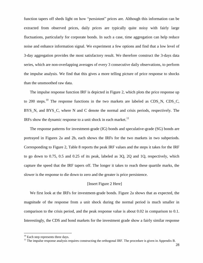
The impulse response function IRF is depicted in Figure 2, which plots the price response up
to 200 steps.10
The response functions in the two markets are labeled as CDS_N, CDS_C,
BYS_N, and BYS_C, where N and C denote the normal and crisis periods, respectively. The
IRFs show the dynamic response to a unit shock in each market.11
The response patterns for investment-grade (IG) bonds and speculative-grade (SG) bonds are
portrayed in Figures 2a and 2b, each shows the IRFs for the two markets in two subperiods.
Corresponding to Figure 2, Table 8 reports the peak IRF values and the steps it takes for the IRF
to go down to 0.75, 0.5 and 0.25 of its peak, labeled as 3Q, 2Q and 1Q, respectively, which
capture the speed that the IRF tapers off. The longer it takes to reach these quartile marks, the
slower is the response to die down to zero and the greater is price persistence.
[Insert Figure 2 Here]
We first look at the IRFs for investment-grade bonds. Figure 2a shows that as expected, the
magnitude of the response from a unit shock during the normal period is much smaller in
comparison to the crisis period, and the peak response value is about 0.02 in comparison to 0.1.
Interestingly, the CDS and bond markets for the investment grade show a fairly similar response
10
Each step represents three days. 11
The impulse response analysis requires constructing the orthogonal IRF. The procedure is given in Appendix B.

29
pattern in both periods with CDS rates somewhat more persistent during the crisis period.
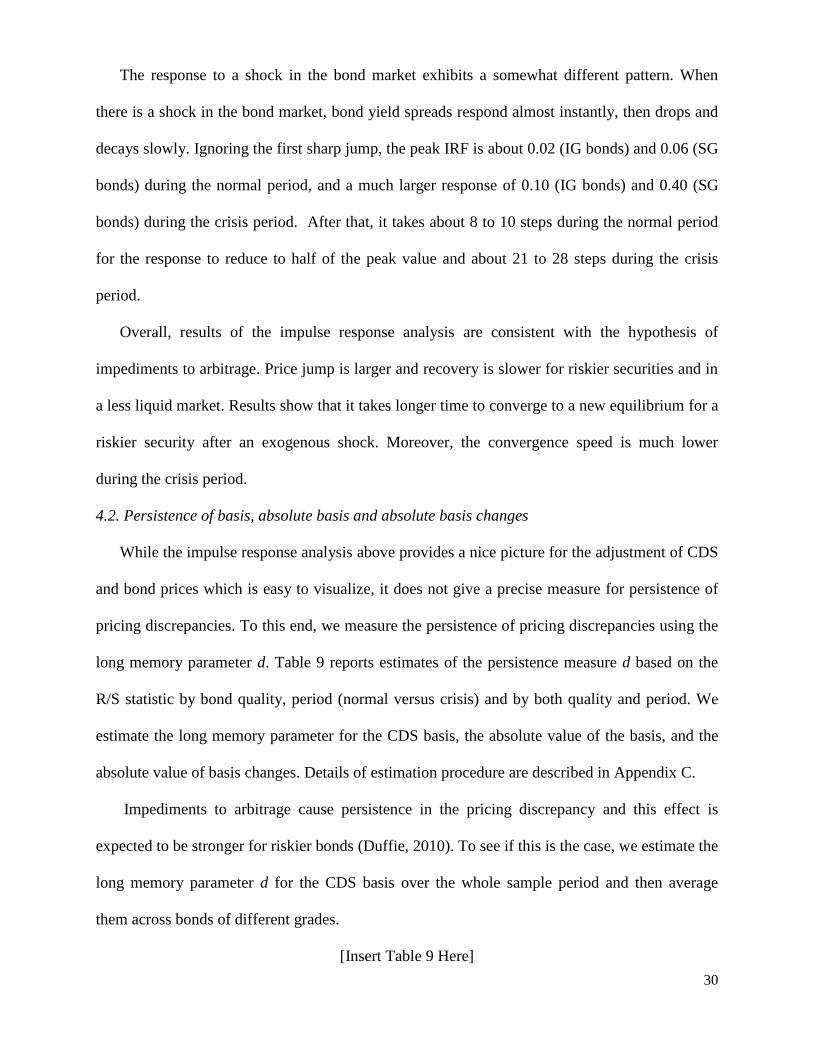
For speculative-grade bonds, Figure 2b gives the impression that the CDS is much more
persistent than the bond market. Looking more closely reveals that there is a sharp initial jump
for the corporate bond spread during the crisis period, which drops rapidly and after that the IRF
tapers off slowly. To better reflect the speed of decay, we ignore the first IRF jump and report
the 3Q, 2Q and 1Q without it in Table 8. The resulting quartile marks for corporate bonds
become quite comparable to those of the CDS during the crisis period. For investment-grade
bonds, the quartile marks for the CDS require 14, 31 and 65 steps to reach and 13, 28 and 61
steps for bonds during the crisis. A similar pattern is found for speculative-grade bonds.
[Insert Table 8 Here]
Results in Figure 2 clearly show that the magnitude of the impulse response is much higher
for speculative-grade bonds than investment-grade bonds. During the normal period, the peak
IRF is around 0.02 for IG bonds and 0.09 for SG bonds. During the crisis period, it is 0.12 for IG
bonds and 0.63 for SG bonds. From Figure 2, it can also be visualized that the speed of CDS
spread adjustment to a shock depends on the riskiness of the reference bond and the condition of
the financial market. The speed of adjustment is somewhat higher for the CDS of IG bonds. As
shown in Table 8, it takes 8, 15 and 25 steps to drop to the quartile marks of the peak response
value for the CDS of SG bonds but it only takes 7, 12, 19 steps for the CDS of IG bonds during
the normal period.
Controlling for the riskiness of the security, the speed of price adjustment is slower when the
market is more uncertain as it is during the crisis period. For example, it takes 31 steps for the
CDS of investment-grade bonds to drop down to the half of the peak response value during the
crisis period, compared to only 12 steps during the normal period. Similarly, for the CDS of
speculatively-grade bonds, it takes 22 steps to drop down to the half of the peak response during
the crisis period, as opposed to 15 steps during the normal period.
30
The response to a shock in the bond market exhibits a somewhat different pattern. When
there is a shock in the bond market, bond yield spreads respond almost instantly, then drops and
decays slowly. Ignoring the first sharp jump, the peak IRF is about 0.02 (IG bonds) and 0.06 (SG
bonds) during the normal period, and a much larger response of 0.10 (IG bonds) and 0.40 (SG
bonds) during the crisis period. After that, it takes about 8 to 10 steps during the normal period
for the response to reduce to half of the peak value and about 21 to 28 steps during the crisis
period.
Overall, results of the impulse response analysis are consistent with the hypothesis of
impediments to arbitrage. Price jump is larger and recovery is slower for riskier securities and in
a less liquid market. Results show that it takes longer time to converge to a new equilibrium for a
riskier security after an exogenous shock. Moreover, the convergence speed is much lower
during the crisis period.
4.2. Persistence of basis, absolute basis and absolute basis changes
While the impulse response analysis above provides a nice picture for the adjustment of CDS
and bond prices which is easy to visualize, it does not give a precise measure for persistence of
pricing discrepancies. To this end, we measure the persistence of pricing discrepancies using the
long memory parameter d. Table 9 reports estimates of the persistence measure d based on the
R/S statistic by bond quality, period (normal versus crisis) and by both quality and period. We
estimate the long memory parameter for the CDS basis, the absolute value of the basis, and the
absolute value of basis changes. Details of estimation procedure are described in Appendix C.
Impediments to arbitrage cause persistence in the pricing discrepancy and this effect is
expected to be stronger for riskier bonds (Duffie, 2010). To see if this is the case, we estimate the
long memory parameter d for the CDS basis over the whole sample period and then average
them across bonds of different grades.
[Insert Table 9 Here]
31
Panel A of Table 9 reports estimates of the long memory parameter d for the full sample, and
tests of the differences of d’s between speculative- and investment-grade bonds. As indicated, all
three persistence measures are higher (ranging from 0.025 to 0.05, for the basis, |basis| and
|∆basis|) for Difference. The bottom row reports the p-value for the test of the difference in mean
d estimates of SG and IG bonds. The null hypothesis is that the two groups have the same mean
of d, against a one-sided alternative that the mean of d for SG bonds is greater than that for IG
bonds. Results show that the null hypothesis is rejected at the 5% significance level for all cases,
supporting the hypothesis that the CDS basis is more persistent in both level and changes for
speculative-grade bonds.
An important question is whether the basis (or |basis|, |∆basis|) is more persistent during the
crisis period. Pricing discrepancies should be more persistent when there are greater
impediments to arbitrage during the crisis period. Panel B of Table 9 reports the estimates for the
two subperiods. Results show that all persistence measures for the basis, |basis| and |∆basis| are
higher during the crisis period. The bottom row reports the p-value of the two-sample t-test on
the difference in d estimates between the two subperiods. The null hypothesis is that the two
subperiods have the same mean of d, against a one-sided alternative that the mean of d during the
crisis period is greater than that during the normal period. Panel B shows that the null hypothesis
is easily rejected with p-values all close to 0. Results strongly support the hypothesis that the
basis is more persistent in both level and change during the crisis period.
Panel C of Table 9 reports results by both bond grade and period. As shown, persistence of
the basis is the lowest (0.34) for IG bonds during the normal period and the highest (0.40) for SG
bonds during the crisis period. In between, persistence measure is about 0.36 for SG bonds
during the normal period and is 0.39 for IG bond during the crisis period. Results show that for
both IG and SG bonds, the basis is more persistent during the crisis period and the difference is
0.042 for the former and 0.043 for the latter, both are highly significant. The basis for SG bonds

32
is more persistent than that for IG bonds, both in the crisis and normal periods. The difference is
0.015 (crisis period) and 0.014 (normal period) but the p values are only 0.15 to 0.22.
Summarizing, our results show that the basis becomes significantly more persistent during
the crisis period and speculative-grade bonds are more persistent than investment-grade bonds.
Comparatively speaking, the basis for SG bonds during the crisis period has the highest
persistence whereas that for IG bonds during the normal period has the lowest.
Results for the absolute basis (|Basis|) and absolute basis changes (|∆Basis|) also show
significantly higher d values during the crisis period. For the absolute basis, the difference
between SG and IG bonds in the normal period is significant at the one percent level. Similar
results are found for the difference in the persistence of absolute basis changes.
Overall, results strongly support the hypothesis that pricing discrepancies become more
persistent during the financial crisis. This finding is consistent with the contention that frictions
to capital movement and arbitrage lead to more persistent pricing discrepancies during the crisis
period. Results show that pricing discrepancies between the CDS and reference bond can persist
over a long period of time, and are more persistent in times of stress. Moreover, pricing
discrepancies are more persistent for riskier bonds.
4.3. Volatility persistence of the basis
The above results for absolute basis changes suggest that volatility of the basis is persistent.
There is a large literature on volatility persistence and this issue can be explored in a more
formal setting. As basis changes exhibit clustering, it is particularly suitable to analyze volatility
persistence in the GARCH framework. In this section, we estimate the long memory FIGARCH
model which admits a long memory structure in conditional volatility. Specifically, we estimate
the MA(1)-FIGARCH(1,1) for basis changes: 11 ttt eecbasis where
2
1 1 0 1(1 ( ) )(1 ) (1 )d
t tB B e B v with 22
ttt ev (see (9) and (10)). We fit this
33
model to the basis series for investment- and speculative-grade bonds.
Table 10 reports estimates of the MA(1)-FIGARCH(1,1) model of basis changes for IG and
SG bonds for the normal and crisis periods. We observe that in normal times, the CDS basis for
both investment- and speculative-grade bonds does not show very significant volatility persistent
behavior. The d estimate is a little over 0.1 and p-value is about 9% to 10%. In contrast, during
the crisis period the CDS basis shows highly significant volatility persistence, particularly for
speculative-grade bonds. The d estimates are 0.74 and 0.97 for the basis of investment- and
speculative-grade bonds, respectively, with p-values close to 0.
[Insert Table 10 Here]
These results are consistent with the findings in Table 9 and support the hypothesis that
impediments to arbitrage lead to persistent pricing discrepancies during the subprime crisis.
Volatility persistence becomes significantly higher during the crisis period. Moreover, the basis
and its volatility for SG bonds are more persistent than for IG bonds in both normal and crisis
periods. The basis and its volatility for SG bonds during the crisis period are most persistent
whereas those for IG bonds during normal period are least persistent.
5. Conclusion
How can two closely related markets have exceedingly large pricing discrepancies? This
important question bears on equilibrium asset pricing and market integration. Our paper
examines this issue using the data of credit markets, which exhibited an extremely negative CDS
basis during the financial crisis. We investigate roles of nondefault risk factors and impediments
to arbitrage in the unusual pricing discrepancies of the CDS and corporate bond markets.
We find that price discrepancies can be explained partly by nondefault risk factors in the
CDS and bond markets. Bond spreads are more sensitive to nondefault factors such as liquidity,
market uncertainty and supply shocks. This contributes to the negative basis during the subprime
crisis. However, we also find that nondefault risk factors can only explain some of the pricing
34
discrepancies between the CDS and corporate bond markets. Empirical evidence suggests that
impediments to arbitrage are the root cause for pricing discrepancies and lack of integration in
the CDS and corporate bond markets.
Our results show that a significant portion of firms reject the hypothesis of cointegration.
Accounting for the effects of nondefault factors reduces the cases of violations in normal market
conditions but the percentage of firms rejecting the hypothesis remains high during the crisis.
Similar findings are obtained by the nonparametric test. Results point to limits-to-arbitrage as the
cause for disintegration between the CDS and the bond markets.
Consistent with the hypothesis of limited arbitrage, we find that firms with high risk and
trading cost and low liquidity are more likely to experience pricing discrepancies in credit
markets. Pricing discrepancies are more persistent for speculative-grade bonds and are more
severe during the subprime crisis. Both the level and volatility of the basis become more
persistent during the crisis period and exhibit long memory. This finding supports Duffie’s
(2010) hypothesis that slow-moving capital and other impediments to arbitrage cause persistence
in pricing discrepancies over longer horizons.

35
Appendix
A. Cointegration Analysis
The cointegration analysis is conducted at the firm’s level for the observed CDS and BYS
series as well as their adjusted spreads based on the regression of spreads on the nondefault
factors such as liquidity, counterparty risk and deleveraging. For the cointegration analysis to be
meaningful, we first need to check if the two spread series are each I(1) non-stationary. Thus, we
first conduct an augmented Dickey-Fuller (ADF) test on each series. If both series accept the null
hypothesis of unit root, we move forward to the cointegration analysis; otherwise, the case will
be left out. In empirical analysis, the ADF test conducted at the 5% and 10% level give similar
results.
We follow Johansen’s methodology to perform the cointegration test. Detailed description
about this method can be found, for example, in Zivot and Wang (2006, Chapter 12) and we
briefly describe the methodology below. Let )',( ttt qpY , where tp and tq are CDS and the
bond yield spreads, respectively, unadjusted or adjusted for the nondefault components. We first
consider a VECM model of the following form:
t
r
i
ititt eYYcY
1
1
1
Based on the rank of the long-run impact matrix , the number of cointegration vector is
determined. Specifically, there are three possibilities: 1) the case of no cointegration vector with
the rank of = 0, in which both series are non-stationary I(1) but they are not cointegrated since
a cointegration vector cannot be found; 2) the case of two cointegration vectors with the rank of
= 2 in which both CDS and BYS are stationary series; 3) the relevant case of one
cointegration vector with the rank of = 1. In the last case, both series are non-stationary I(1)
but a linear combination of them is stationary; therefore 'b , and )',1( b is the
normalized cointegration vector.
36
We use Johansen’s trace test to draw the inference. The methodology is a sequential test
procedure. Step 1 tests Ho: no cointegration vector versus Ha: at least 1 cointegration vector. If
Ho is not rejected, then no cointegration vector is concluded. If Ho is rejected, step 2 further tests
if there are one or two cointegration vectors; i.e., Ho: 1 cointegration vector versus Ha: 2
cointegration vector. Thus, to conclude one cointegration vector, the trace test statistic has to be
significantly large in step 1 and is significantly small in step 2. Details and critical values are
discussed in Zivot and Wang (2006, Chapter 12).
B. Impulse Response Analysis
For the impulse response analysis, we use the orthogonal impulse response function (IRF) to
study the speed of dynamic response to a unit shock in each market. The approach is briefly
described as follows.12
Let )',( ttt qpY be a vector of bivariate price series which follows a
VAR model: t
r
i
itit eYcY
1
. The error te is a zero-mean vector of serially uncorrelated
innovations with a covariance matrix , which is not necessarily diagonal. In our estimation, the
order of the VAR model use is two. To study the impulse response, a unit shock is introduced to
the system. Specifically, let te = (1,0) or (0,1) be a unit shock occurred in the CDS or the bond
market. The impulse response can be computed based on the estimated VAR model. However,
the impulse response computed this way has the right interpretation only when the covariance
matrix is diagonal, a condition which in practice is seldom met. In the literature, a common
practice is to first diagonalize and then use the transformed VAR model to compute the
(orthogonal) impulse response.
For the two series that we analyze, the CDS has a much higher information share and so we
put it as the first series tp and the BYS as the second series tq . Note that the impulse response
pattern depends on the imposed ordering. The series is then transformed using a lower triangular
12
See Zivot and Wang (2006, Chapter 11) for details.
37
matrix B with a unit diagonal: t
r
i
itit YdBY
1
such that the error term t is orthogonal
and has a diagonal covariance matrix. This triangular structural VAR model can be re-expressed
in an infinite VMA based on the orthogonal error t as ...22110 tttt aY ,
where the diagonal iith element of s can be regarded as the orthogonal impulse response
function (IRF) of the price with respect to the orthogonal error t in the ith market, which
represents the effect on the price sth period later for a unit shock in t .
C. The Procedure for Estimating the Long memory Parameter
We take the following approach to estimate persistence and perform significance tests. In the
time-series literature, it is well known that the persistence behavior, i.e., the long memory
parameter d, is preserved upon time aggregation13
(see for example, Tschernig, 1995; Chambers,
1998; Tsai and Chan, 2005; Man and Tiao, 2006). Time aggregates refer to the non-overlapping
sums (or averages which we use here to maintain the magnitude) of the underlying data. For
instance, weekly and monthly data are time aggregates of daily data, with the level of
aggregation 7 and 30, respectively. Theoretically, they all share the same persistence behavior d.
We utilize this important property to construct our persistence estimate. Specifically, we use the
R/S method to estimate d for each bond rating portfolio based on the underlying daily data, and
its time aggregates from 2 to 10 days. For each rating portfolio, we obtain ten d estimates and
the average of these d values is used as the persistence measure. We find that this approach
yields a more stable persistence estimate. Results are then summarized into speculative- and
investment-grade bond groups. We use this procedure to obtain the persistence measure for the
whole sample period and the normal and crisis periods, respectively.
13
Ohanissian, Russell and Tsay (2008) use this invariance property to propose a statistical test to distinguish
between true long memory and spurious long memory.
38
References
Amihud, Y., 2002. Illiquidity and stock returns: cross section and time series effects. Journal of
Financial Markets 5, 31–56.
Arora, N., Gandhi, P., Longstaff, F. A., 2012. Counterparty credit risk and the credit default
swap market. Journal of Financial Economics 103, 280–293.
Bai, J., Collin-Dufresne, P., 2013. The CDS-Bond Basis during the Financial Crisis of 2007-
2009, 2013 AFA Conference paper.
Baillie, R.T., Bollerslev, T., and Mikkelsen, H.O., 1996, Fractionally integrated generalized
autoregressive conditional heteroskedasticity. Journal of Econometrics 74, 3-30.
Bakshi, G., Cao, C., Chen, Z., 2000. Do call prices and the underlying stock always move in the
same direction? Review of Financial Studies 13, 549-584.
Blanco, R., Brennan, S., Marsh, I. W., 2005. An empirical analysis of the dynamic relation
between investment-grade bonds and credit default swaps. Journal of Finance 60, 2255-2281.
Bongaerts, D., de Jong, F., Driessen, J., 2011. Derivative pricing with liquidity risk: Theory and
evidence from the credit default swap market. Journal of Finance 66, 203-240.
Chambers, M., 1998. Long memory and aggregation in macroeconomic time series. International
Economic Review 39, 1053– 1072.
Collin-Dufresne, P., Goldstein, R. S., Martin, J. S., 2001. The determinants of credit spread
changes. Journal of Finance 56, 2177–2207.
Das, S., Kalimipalli, M., Nayak, S., 2013. Did CDS trading improves the market for corporate
bonds? Journal of Financial Economics, forthcoming.
Dick-Nielsen, J., Feldhutter, P., Lando, D., 2012. Corporate bond liquidity before and after the
onset of the subprime crisis. Journal of Financial Economics 103, 471-492.
Duffie, D., 1999. Credit swap valuation. Financial Analyst Journal 55, 73-87.
Duffie, D., 2010. Presidential address: Asset price dynamics with slow-moving capital. Journal
of Finance 4, 1237-1267.
Friewald, N., Jankowitsch, R., Subrahmanyam, M., 2012. Illiquidity or credit deterioration: A
study of liquidity in the US corporate bond market during financial crises. Journal of
Financial Economics 150, 18-36.
Gonzalo, J., Granger, C., 1995. Estimation of common long memory components in cointegrated
systems. Journal of Business and Economic Statistics 13, 27-35.
Gorton, G., Metrick, A., 2012. Securitized banking and the run on repo. Journal of Financial
Economics
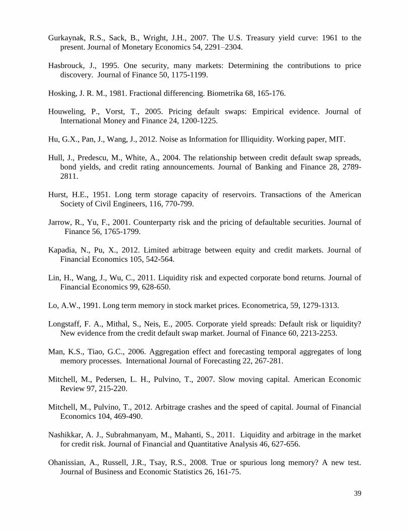
39
Gurkaynak, R.S., Sack, B., Wright, J.H., 2007. The U.S. Treasury yield curve: 1961 to the
present. Journal of Monetary Economics 54, 2291–2304.
Hasbrouck, J., 1995. One security, many markets: Determining the contributions to price
discovery. Journal of Finance 50, 1175-1199.
Hosking, J. R. M., 1981. Fractional differencing. Biometrika 68, 165-176.
Houweling, P., Vorst, T., 2005. Pricing default swaps: Empirical evidence. Journal of
International Money and Finance 24, 1200-1225.
Hu, G.X., Pan, J., Wang, J., 2012. Noise as Information for Illiquidity. Working paper, MIT.
Hull, J., Predescu, M., White, A., 2004. The relationship between credit default swap spreads,
bond yields, and credit rating announcements. Journal of Banking and Finance 28, 2789-
2811.
Hurst, H.E., 1951. Long term storage capacity of reservoirs. Transactions of the American
Society of Civil Engineers, 116, 770-799.
Jarrow, R., Yu, F., 2001. Counterparty risk and the pricing of defaultable securities. Journal of
Finance 56, 1765-1799.
Kapadia, N., Pu, X., 2012. Limited arbitrage between equity and credit markets. Journal of
Financial Economics 105, 542-564.
Lin, H., Wang, J., Wu, C., 2011. Liquidity risk and expected corporate bond returns. Journal of
Financial Economics 99, 628-650.
Lo, A.W., 1991. Long term memory in stock market prices. Econometrica, 59, 1279-1313.
Longstaff, F. A., Mithal, S., Neis, E., 2005. Corporate yield spreads: Default risk or liquidity?
New evidence from the credit default swap market. Journal of Finance 60, 2213-2253.
Man, K.S., Tiao, G.C., 2006. Aggregation effect and forecasting temporal aggregates of long
memory processes. International Journal of Forecasting 22, 267-281.
Mitchell, M., Pedersen, L. H., Pulvino, T., 2007. Slow moving capital. American Economic
Review 97, 215-220.
Mitchell, M., Pulvino, T., 2012. Arbitrage crashes and the speed of capital. Journal of Financial
Economics 104, 469-490.
Nashikkar, A. J., Subrahmanyam, M., Mahanti, S., 2011. Liquidity and arbitrage in the market
for credit risk. Journal of Financial and Quantitative Analysis 46, 627-656.
Ohanissian, A., Russell, J.R., Tsay, R.S., 2008. True or spurious long memory? A new test.
Journal of Business and Economic Statistics 26, 161-75.
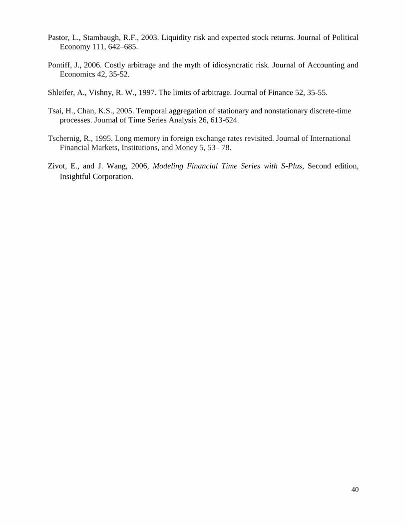
40
Pastor, L., Stambaugh, R.F., 2003. Liquidity risk and expected stock returns. Journal of Political
Economy 111, 642–685.
Pontiff, J., 2006. Costly arbitrage and the myth of idiosyncratic risk. Journal of Accounting and
Economics 42, 35-52.
Shleifer, A., Vishny, R. W., 1997. The limits of arbitrage. Journal of Finance 52, 35-55.
Tsai, H., Chan, K.S., 2005. Temporal aggregation of stationary and nonstationary discrete-time
processes. Journal of Time Series Analysis 26, 613-624.
Tschernig, R., 1995. Long memory in foreign exchange rates revisited. Journal of International
Financial Markets, Institutions, and Money 5, 53– 78.
Zivot, E., and J. Wang, 2006, Modeling Financial Time Series with S-Plus, Second edition,
Insightful Corporation.
41
Figure 1: Average basis and residuals (risk-adjusted basis) from 2005 to 2009.
This figure plots mean observed basis and the basis adjusted for the effects of nondefault factors in percentage. Figure 1a is for the investment-
grade firms, figure 1b is for the speculative-grade firms, and figure 1c is for all firms.
-3.5
-3.0
-2.5
-2.0
-1.5
-1.0
-0.5
0.0
0.5
1.0
1.5
2005 2005 2006 2006 2007 2007 2008 2008 2009
Average Basis Average Residual
Figure 1A: Investment Grade Bonds
-3.5
-3.0
-2.5
-2.0
-1.5
-1.0
-0.5
0.0
0.5
1.0
1.5
2005 2005 2006 2006 2007 2007 2008 2008 2009
Average Basis Average Residual
Figure 1B: Speculative Grade Bonds
-3.5
-3.0
-2.5
-2.0
-1.5
-1.0
-0.5
0.0
0.5
1.0
1.5
2005 2005 2006 2006 2007 2007 2008 2008 2009
Average Basis Average Residual
Figure 1C: All Bonds
42
Figure 2. Impulse Response
The graphs show the speed and dynamic responses to a unit shock in the CDS and bond markets
during the normal and crisis periods. We plot the orthogonal IRF (vertical axis) up to 200 steps
(horizontal axis) based on 3-day data, each step represents three days. The graph shows the
orthogonal IRF of CDS during normal period (CDS_N) and crisis period (CDS_C), and similarly
for bond yield spreads BYS_N and BYS_C, resulting from a unit shock in their own market. The
IRF is computed based on the estimates of the VAR model. Figure 2a is for investment-grade
bonds, while Figure 2b is for speculative-grade bonds. The two higher response curves
correspond to the crisis period.
2a. Investment-grade bonds
2b. Speculative-grade bonds
0
0.02
0.04
0.06
0.08
0.1
0.12
0.14
1
12
23
34
45
56
67
78
89
10
0
11
1
12
2
13
3
14
4
15
5
16
6
17
7
18
8
19
9
CDS_N
CDS_C
BYS_N
BYS_C
-0.1
0
0.1
0.2
0.3
0.4
0.5
0.6
0.7
0.8
1
12
23
34
45
56
67
78
89
10
0
11
1
12
2
13
3
14
4
15
5
16
6
17
7
18
8
19
9
CDS_N
CDS_C
BYS_N
BYS_C
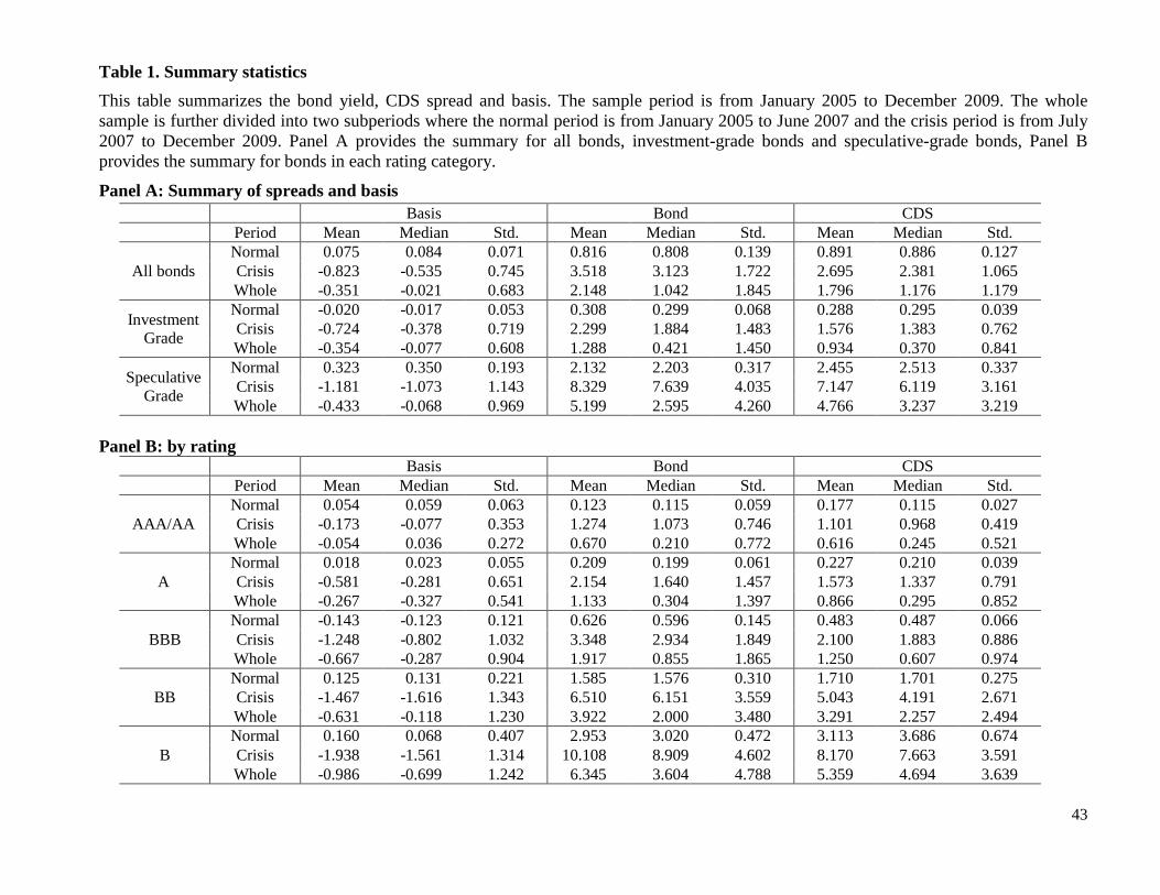
43
Table 1. Summary statistics
This table summarizes the bond yield, CDS spread and basis. The sample period is from January 2005 to December 2009. The whole
sample is further divided into two subperiods where the normal period is from January 2005 to June 2007 and the crisis period is from July
2007 to December 2009. Panel A provides the summary for all bonds, investment-grade bonds and speculative-grade bonds, Panel B
provides the summary for bonds in each rating category.
Panel A: Summary of spreads and basis
Basis Bond CDS
Period Mean Median Std. Mean Median Std. Mean Median Std.
All bonds
Normal 0.075 0.084 0.071 0.816 0.808 0.139 0.891 0.886 0.127
Crisis -0.823 -0.535 0.745 3.518 3.123 1.722 2.695 2.381 1.065
Whole -0.351 -0.021 0.683 2.148 1.042 1.845 1.796 1.176 1.179
Investment
Grade
Normal -0.020 -0.017 0.053 0.308 0.299 0.068 0.288 0.295 0.039
Crisis -0.724 -0.378 0.719 2.299 1.884 1.483 1.576 1.383 0.762
Whole -0.354 -0.077 0.608 1.288 0.421 1.450 0.934 0.370 0.841
Speculative
Grade
Normal 0.323 0.350 0.193 2.132 2.203 0.317 2.455 2.513 0.337
Crisis -1.181 -1.073 1.143 8.329 7.639 4.035 7.147 6.119 3.161
Whole -0.433 -0.068 0.969 5.199 2.595 4.260 4.766 3.237 3.219
Panel B: by rating Basis Bond CDS
Period Mean Median Std. Mean Median Std. Mean Median Std.
AAA/AA
Normal 0.054 0.059 0.063 0.123 0.115 0.059 0.177 0.115 0.027
Crisis -0.173 -0.077 0.353 1.274 1.073 0.746 1.101 0.968 0.419
Whole -0.054 0.036 0.272 0.670 0.210 0.772 0.616 0.245 0.521
A
Normal 0.018 0.023 0.055 0.209 0.199 0.061 0.227 0.210 0.039
Crisis -0.581 -0.281 0.651 2.154 1.640 1.457 1.573 1.337 0.791
Whole -0.267 -0.327 0.541 1.133 0.304 1.397 0.866 0.295 0.852
BBB
Normal -0.143 -0.123 0.121 0.626 0.596 0.145 0.483 0.487 0.066
Crisis -1.248 -0.802 1.032 3.348 2.934 1.849 2.100 1.883 0.886
Whole -0.667 -0.287 0.904 1.917 0.855 1.865 1.250 0.607 0.974
BB
Normal 0.125 0.131 0.221 1.585 1.576 0.310 1.710 1.701 0.275
Crisis -1.467 -1.616 1.343 6.510 6.151 3.559 5.043 4.191 2.671
Whole -0.631 -0.118 1.230 3.922 2.000 3.480 3.291 2.257 2.494
B
Normal 0.160 0.068 0.407 2.953 3.020 0.472 3.113 3.686 0.674
Crisis -1.938 -1.561 1.314 10.108 8.909 4.602 8.170 7.663 3.591
Whole -0.986 -0.699 1.242 6.345 3.604 4.788 5.359 4.694 3.639
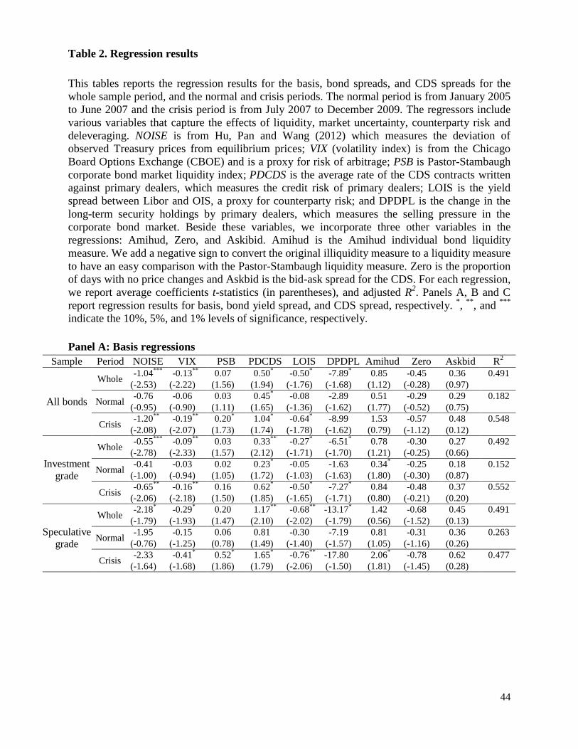
44
Table 2. Regression results
This tables reports the regression results for the basis, bond spreads, and CDS spreads for the
whole sample period, and the normal and crisis periods. The normal period is from January 2005
to June 2007 and the crisis period is from July 2007 to December 2009. The regressors include
various variables that capture the effects of liquidity, market uncertainty, counterparty risk and
deleveraging. NOISE is from Hu, Pan and Wang (2012) which measures the deviation of
observed Treasury prices from equilibrium prices; VIX (volatility index) is from the Chicago
Board Options Exchange (CBOE) and is a proxy for risk of arbitrage; PSB is Pastor-Stambaugh
corporate bond market liquidity index; PDCDS is the average rate of the CDS contracts written
against primary dealers, which measures the credit risk of primary dealers; LOIS is the yield
spread between Libor and OIS, a proxy for counterparty risk; and DPDPL is the change in the
long-term security holdings by primary dealers, which measures the selling pressure in the
corporate bond market. Beside these variables, we incorporate three other variables in the
regressions: Amihud, Zero, and Askibid. Amihud is the Amihud individual bond liquidity
measure. We add a negative sign to convert the original illiquidity measure to a liquidity measure
to have an easy comparison with the Pastor-Stambaugh liquidity measure. Zero is the proportion
of days with no price changes and Askbid is the bid-ask spread for the CDS. For each regression,
we report average coefficients t-statistics (in parentheses), and adjusted R2. Panels A, B and C
report regression results for basis, bond yield spread, and CDS spread, respectively. *,
**, and
***
indicate the 10%, 5%, and 1% levels of significance, respectively.
Panel A: Basis regressions
Sample Period NOISE VIX PSB PDCDS LOIS DPDPL Amihud Zero Askbid R2
All bonds
Whole -1.04
*** -0.13
** 0.07 0.50
* -0.50
* -7.89
* 0.85 -0.45 0.36 0.491
(-2.53) (-2.22) (1.56) (1.94) (-1.76) (-1.68) (1.12) (-0.28) (0.97)
Normal -0.76 -0.06 0.03 0.45
* -0.08 -2.89 0.51 -0.29 0.29 0.182
(-0.95) (-0.90) (1.11) (1.65) (-1.36) (-1.62) (1.77) (-0.52) (0.75)
Crisis -1.20
** -0.19
** 0.20
* 1.04
* -0.64
* -8.99 1.53 -0.57 0.48 0.548
(-2.08) (-2.07) (1.73) (1.74) (-1.78) (-1.62) (0.79) (-1.12) (0.12)
Investment
grade
Whole -0.55
*** -0.09
** 0.03 0.33
** -0.27
* -6.51
* 0.78 -0.30 0.27 0.492
(-2.78) (-2.33) (1.57) (2.12) (-1.71) (-1.70) (1.21) (-0.25) (0.66)
Normal -0.41 -0.03 0.02 0.23
* -0.05 -1.63 0.34
* -0.25 0.18 0.152
(-1.00) (-0.94) (1.05) (1.72) (-1.03) (-1.63) (1.80) (-0.30) (0.87)
Crisis -0.65
** -0.16
** 0.16 0.62
* -0.50
* -7.27
* 0.84 -0.48 0.37 0.552
(-2.06) (-2.18) (1.50) (1.85) (-1.65) (-1.71) (0.80) (-0.21) (0.20)
Speculative
grade
Whole -2.18
* -0.29
* 0.20 1.17
** -0.68
** -13.17
* 1.42 -0.68 0.45 0.491
(-1.79) (-1.93) (1.47) (2.10) (-2.02) (-1.79) (0.56) (-1.52) (0.13)
Normal -1.95 -0.15 0.06 0.81 -0.30 -7.19 0.81 -0.31 0.36 0.263
(-0.76) (-1.25) (0.78) (1.49) (-1.40) (-1.57) (1.05) (-1.16) (0.26)
Crisis -2.33 -0.41
* 0.52
* 1.65
* -0.76
** -17.80 2.06
* -0.78 0.62 0.477
(-1.64) (-1.68) (1.86) (1.79) (-2.06) (-1.50) (1.81) (-1.45) (0.28)
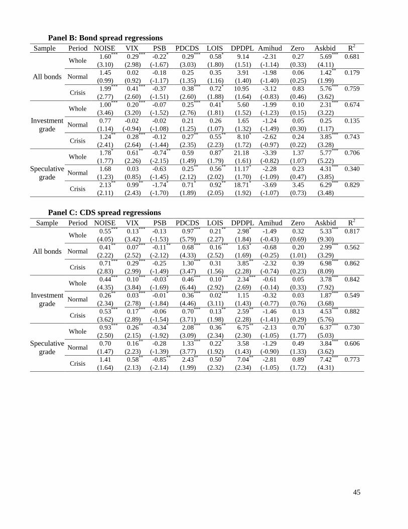
45
Panel B: Bond spread regressions
Sample Period NOISE VIX PSB PDCDS LOIS DPDPL Amihud Zero Askbid R2
All bonds
Whole 1.60
*** 0.29
*** -0.22
* 0.29
*** 0.58
* 9.14 -2.31 0.27 5.69
*** 0.681
(3.10) (2.98) (-1.67) (3.03) (1.80) (1.51) (-1.14) (0.33) (4.11)
Normal 1.45 0.02 -0.18 0.25 0.35 3.91 -1.98 0.06 1.42
** 0.179
(0.99) (0.92) (-1.17) (1.35) (1.16) (1.40) (-1.40) (0.25) (1.99)
Crisis 1.99
*** 0.41
*** -0.37 0.38
*** 0.72
* 10.95 -3.12 0.83 5.76
*** 0.759
(2.77) (2.60) (-1.51) (2.60) (1.88) (1.64) (-0.83) (0.46) (3.62)
Investment
grade
Whole 1.00
*** 0.20
*** -0.07 0.25
*** 0.41
* 5.60 -1.99 0.10 2.31
*** 0.674
(3.46) (3.20) (-1.52) (2.76) (1.81) (1.52) (-1.23) (0.15) (3.22)
Normal 0.77 -0.02 -0.02 0.21 0.26 1.65 -1.24 0.05 0.25 0.135
(1.14) (-0.94) (-1.08) (1.25) (1.07) (1.32) (-1.49) (0.30) (1.17)
Crisis 1.24
** 0.28
*** -0.12 0.27
** 0.55
** 8.10
* -2.62 0.24 3.85
*** 0.743
(2.41) (2.64) (-1.44) (2.35) (2.23) (1.72) (-0.97) (0.22) (3.28)
Speculative
grade
Whole 1.78
* 0.61
** -0.74
** 0.59 0.87
* 21.18 -3.39 1.37 5.77
*** 0.706
(1.77) (2.26) (-2.15) (1.49) (1.79) (1.61) (-0.82) (1.07) (5.22)
Normal 1.68 0.03 -0.63 0.25
** 0.56
** 11.17
* -2.28 0.23 4.31
*** 0.340
(1.23) (0.85) (-1.45) (2.12) (2.02) (1.70) (-1.09) (0.47) (3.85)
Crisis 2.13
** 0.99
** -1.74
* 0.71
* 0.92
** 18.71
* -3.69 3.45 6.29
*** 0.829
(2.11) (2.43) (-1.70) (1.89) (2.05) (1.92) (-1.07) (0.73) (3.48)
Panel C: CDS spread regressions
Sample Period NOISE VIX PSB PDCDS LOIS DPDPL Amihud Zero Askbid R2
All bonds
Whole 0.55
*** 0.13
*** -0.13 0.97
*** 0.21
** 2.98
* -1.49 0.32 5.33
*** 0.817
(4.05) (3.42) (-1.53) (5.79) (2.27) (1.84) (-0.43) (0.69) (9.30)
Normal 0.41
** 0.07
*** -0.11
** 0.68
*** 0.16
*** 1.63
* -0.68 0.20 2.99
*** 0.562
(2.22) (2.52) (-2.12) (4.33) (2.52) (1.69) (-0.25) (1.01) (3.29)
Crisis 0.71
*** 0.29
*** -0.25 1.30
*** 0.31 3.85
** -2.32 0.39 6.98
*** 0.862
(2.83) (2.99) (-1.49) (3.47) (1.56) (2.28) (-0.74) (0.23) (8.09)
Investment
grade
Whole 0.44
*** 0.10
*** -0.03
* 0.46
*** 0.10
*** 2.34
*** -0.61 0.05 3.78
*** 0.842
(4.35) (3.84) (-1.69) (6.44) (2.92) (2.69) (-0.14) (0.33) (7.92)
Normal 0.26
** 0.03
*** -0.01
* 0.36
*** 0.02
*** 1.15 -0.32 0.03 1.87
*** 0.549
(2.34) (2.78) (-1.84) (4.46) (3.11) (1.43) (-0.77) (0.76) (3.68)
Crisis 0.53
*** 0.17
*** -0.06 0.70
*** 0.13
** 2.59
** -1.46 0.13 4.53
*** 0.882
(3.62) (2.89) (-1.54) (3.71) (1.98) (2.28) (-1.41) (0.29) (5.76)
Speculative
grade
Whole 0.93
*** 0.26
** -0.34
* 2.08
*** 0.36
** 6.75
** -2.13 0.70
* 6.37
*** 0.730
(2.50) (2.15) (-1.92) (3.09) (2.34) (2.30) (-1.05) (1.77) (5.03)
Normal 0.70 0.16
** -0.28 1.33
*** 0.22
* 3.58 -1.29 0.49 3.84
*** 0.606
(1.47) (2.23) (-1.39) (3.77) (1.92) (1.43) (-0.90) (1.33) (3.62)
Crisis 1.41 0.58
** -0.85
** 2.43
** 0.50
** 7.04
** -2.81 0.89
* 7.42
*** 0.773
(1.64) (2.13) (-2.14) (1.99) (2.32) (2.34) (-1.05) (1.72) (4.31)
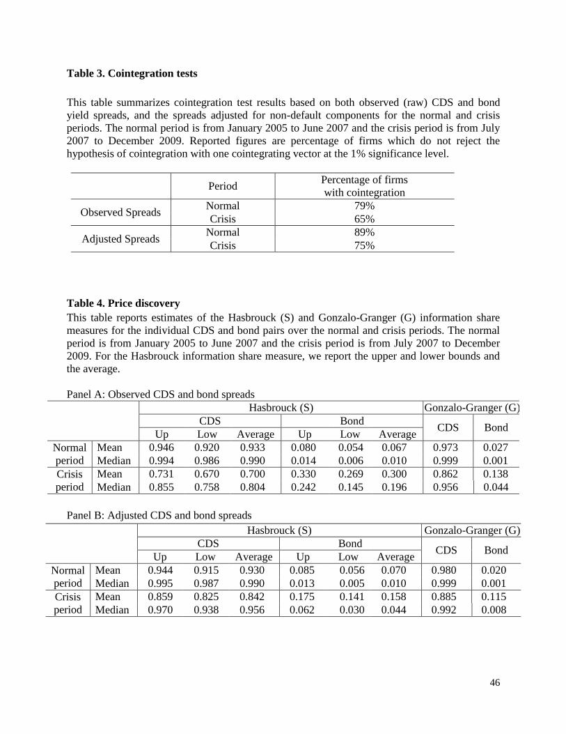
46
Table 3. Cointegration tests
This table summarizes cointegration test results based on both observed (raw) CDS and bond
yield spreads, and the spreads adjusted for non-default components for the normal and crisis
periods. The normal period is from January 2005 to June 2007 and the crisis period is from July
2007 to December 2009. Reported figures are percentage of firms which do not reject the
hypothesis of cointegration with one cointegrating vector at the 1% significance level.
Period Percentage of firms
with cointegration
Observed Spreads Normal 79%
Crisis 65%
Adjusted Spreads Normal 89%
Crisis 75%
Table 4. Price discovery
This table reports estimates of the Hasbrouck (S) and Gonzalo-Granger (G) information share
measures for the individual CDS and bond pairs over the normal and crisis periods. The normal
period is from January 2005 to June 2007 and the crisis period is from July 2007 to December
2009. For the Hasbrouck information share measure, we report the upper and lower bounds and
the average.
Panel A: Observed CDS and bond spreads
Hasbrouck (S) Gonzalo-Granger (G)
CDS Bond CDS Bond
Up Low Average Up Low Average
Normal
period
Mean 0.946 0.920 0.933 0.080 0.054 0.067 0.973 0.027
Median 0.994 0.986 0.990 0.014 0.006 0.010 0.999 0.001
Crisis
period
Mean 0.731 0.670 0.700 0.330 0.269 0.300 0.862 0.138
Median 0.855 0.758 0.804 0.242 0.145 0.196 0.956 0.044
Panel B: Adjusted CDS and bond spreads
Hasbrouck (S) Gonzalo-Granger (G)
CDS Bond CDS Bond
Up Low Average Up Low Average
Normal
period
Mean 0.944 0.915 0.930 0.085 0.056 0.070 0.980 0.020
Median 0.995 0.987 0.990 0.013 0.005 0.010 0.999 0.001
Crisis
period
Mean 0.859 0.825 0.842 0.175 0.141 0.158 0.885 0.115
Median 0.970 0.938 0.956 0.062 0.030 0.044 0.992 0.008
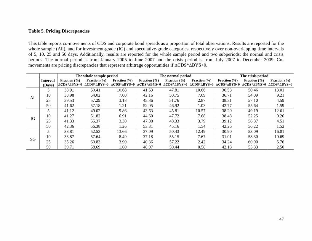
47
Table 5. Pricing Discrepancies
This table reports co-movements of CDS and corporate bond spreads as a proportion of total observations. Results are reported for the
whole sample (All), and for investment-grade (IG) and speculative-grade categories, respectively over non-overlapping time intervals
of 5, 10, 25 and 50 days. Additionally, results are reported for the whole sample period and two subperiods: the normal and crisis
periods. The normal period is from January 2005 to June 2007 and the crisis period is from July 2007 to December 2009. Co-
movements are pricing discrepancies that represent arbitrage opportunities if ∆CDS*∆BYS>0.
The whole sample period The normal period The crisis period
Interval
(Days) Fraction (%)
∆CDS*∆BYS<0 Fraction (%)
∆CDS*∆BYS>0
Fraction (%)
∆CDS*∆BYS=0
Fraction (%)
∆CDS*∆BYS<0 Fraction (%)
∆CDS*∆BYS>0
Fraction (%)
∆CDS*∆BYS=0
Fraction (%)
∆CDS*∆BYS<0 Fraction (%)
∆CDS*∆BYS>0
Fraction (%)
∆CDS*∆BYS=0
All
5 38.91 50.41 10.68 41.53 47.81 10.66 36.53 50.46 13.01
10 38.98 54.02 7.00 42.16 50.75 7.09 36.71 54.09 9.21
25 39.53 57.29 3.18 45.36 51.76 2.87 38.31 57.10 4.59
50 41.62 57.18 1.21 52.05 46.92 1.03 42.77 55.64 1.59
IG
5 41.12 49.02 9.86 43.63 45.81 10.57 38.20 49.19 12.61
10 41.27 51.82 6.91 44.60 47.72 7.68 38.48 52.25 9.26
25 41.33 55.37 3.30 47.88 48.33 3.79 39.12 56.37 4.51
50 42.36 56.38 1.26 53.31 45.16 1.54 42.26 56.22 1.52
SG
5 33.81 52.53 13.66 37.09 50.43 12.49 30.90 53.09 16.01
10 33.87 57.64 8.49 37.18 55.15 7.67 31.01 58.30 10.69
25 35.26 60.83 3.90 40.36 57.22 2.42 34.24 60.00 5.76
50 39.71 58.69 1.60 48.97 50.44 0.58 42.18 55.33 2.50
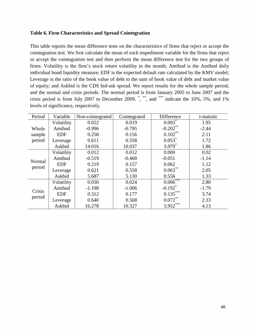
48
Table 6. Firm Characteristics and Spread Cointegration
This table reports the mean difference tests on the characteristics of firms that reject or accept the
cointegration test. We first calculate the mean of each impediment variable for the firms that reject
or accept the cointegration test and then perform the mean difference test for the two groups of
firms. Volatility is the firm’s stock return volatility in the month; Amihud is the Amihud daily
individual bond liquidity measure; EDF is the expected default rate calculated by the KMV model;
Leverage is the ratio of the book value of debt to the sum of book value of debt and market value
of equity; and Askbid is the CDS bid-ask spread. We report results for the whole sample period,
and the normal and crisis periods. The normal period is from January 2005 to June 2007 and the
crisis period is from July 2007 to December 2009. *,
**, and
*** indicate the 10%, 5%, and 1%
levels of significance, respectively.
Period Variable Non-cointegrated Cointegrated Difference t-statistic
Whole
sample
period
Volatility 0.022 0.019 0.003* 1.95
Amihud -0.996 -0.795 -0.202**
-2.44
EDF 0.258 0.156 0.102**
2.11
Leverage 0.611 0.558 0.053* 1.72
Askbid 14.016 10.037 3.979* 1.86
Normal
period
Volatility 0.012 0.012 0.000 0.02
Amihud -0.519 -0.468 -0.051 -1.14
EDF 0.219 0.157 0.062 1.12
Leverage 0.621 0.558 0.063**
2.05
Askbid 5.687 5.130 0.556 1.33
Crisis
period
Volatility 0.030 0.024 0.006***
2.80
Amihud -1.198 -1.006 -0.192* -1.79
EDF 0.312 0.177 0.135***
3.74
Leverage 0.640 0.568 0.072**
2.33
Askbid 16.278 10.327 5.952***
4.13
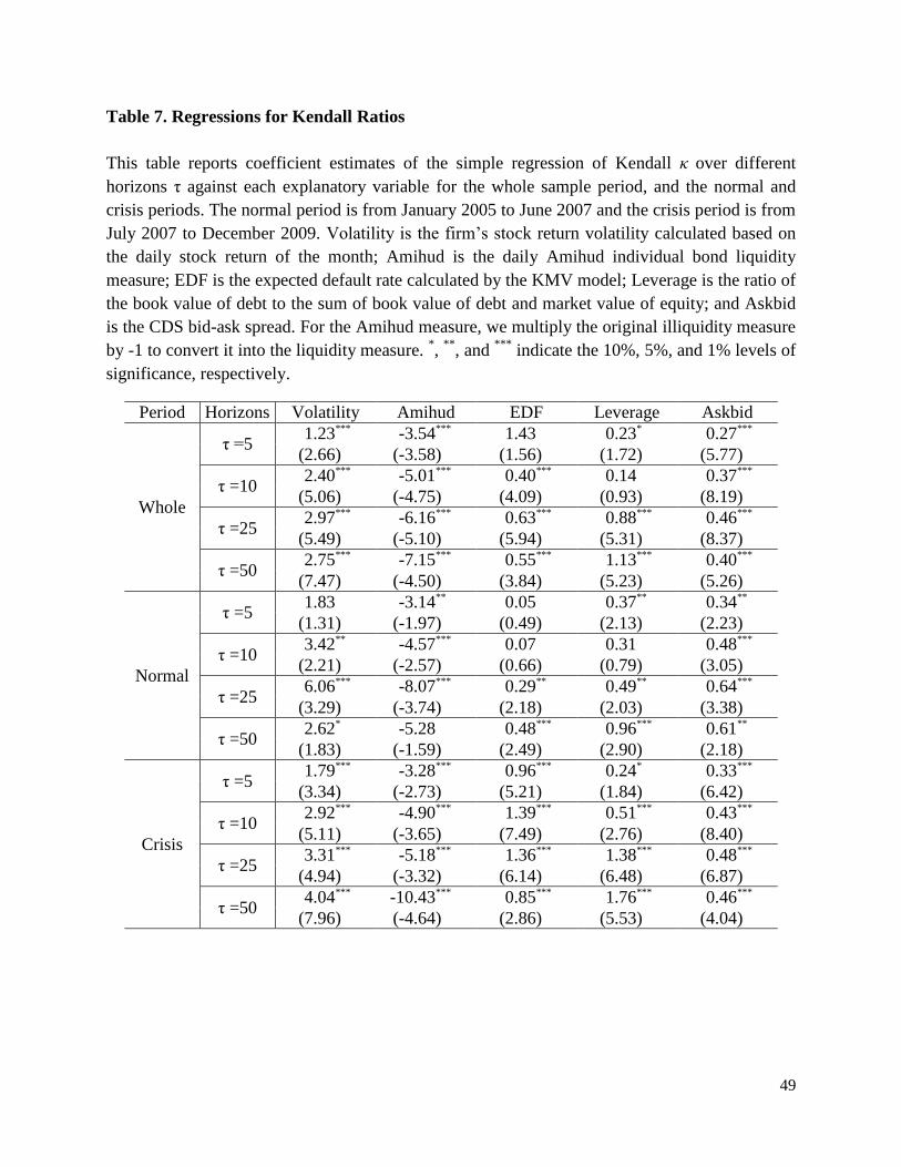
49
Table 7. Regressions for Kendall Ratios
This table reports coefficient estimates of the simple regression of Kendall κ over different
horizons τ against each explanatory variable for the whole sample period, and the normal and
crisis periods. The normal period is from January 2005 to June 2007 and the crisis period is from
July 2007 to December 2009. Volatility is the firm’s stock return volatility calculated based on
the daily stock return of the month; Amihud is the daily Amihud individual bond liquidity
measure; EDF is the expected default rate calculated by the KMV model; Leverage is the ratio of
the book value of debt to the sum of book value of debt and market value of equity; and Askbid
is the CDS bid-ask spread. For the Amihud measure, we multiply the original illiquidity measure
by -1 to convert it into the liquidity measure. *,
**, and
*** indicate the 10%, 5%, and 1% levels of
significance, respectively.
Period Horizons Volatility Amihud EDF Leverage Askbid
Whole
τ =5 1.23*** -3.54*** 1.43 0.23* 0.27***
(2.66) (-3.58) (1.56) (1.72) (5.77)
τ =10 2.40*** -5.01*** 0.40*** 0.14 0.37***
(5.06) (-4.75) (4.09) (0.93) (8.19)
τ =25 2.97*** -6.16*** 0.63*** 0.88*** 0.46***
(5.49) (-5.10) (5.94) (5.31) (8.37)
τ =50 2.75*** -7.15*** 0.55*** 1.13*** 0.40***
(7.47) (-4.50) (3.84) (5.23) (5.26)
Normal
τ =5 1.83 -3.14** 0.05 0.37** 0.34**
(1.31) (-1.97) (0.49) (2.13) (2.23)
τ =10 3.42** -4.57*** 0.07 0.31 0.48***
(2.21) (-2.57) (0.66) (0.79) (3.05)
τ =25 6.06*** -8.07*** 0.29** 0.49** 0.64***
(3.29) (-3.74) (2.18) (2.03) (3.38)
τ =50 2.62* -5.28 0.48*** 0.96*** 0.61**
(1.83) (-1.59) (2.49) (2.90) (2.18)
Crisis
τ =5 1.79*** -3.28*** 0.96*** 0.24* 0.33***
(3.34) (-2.73) (5.21) (1.84) (6.42)
τ =10 2.92*** -4.90*** 1.39*** 0.51*** 0.43***
(5.11) (-3.65) (7.49) (2.76) (8.40)
τ =25 3.31*** -5.18*** 1.36*** 1.38*** 0.48***
(4.94) (-3.32) (6.14) (6.48) (6.87)
τ =50 4.04*** -10.43*** 0.85*** 1.76*** 0.46***
(7.96) (-4.64) (2.86) (5.53) (4.04)
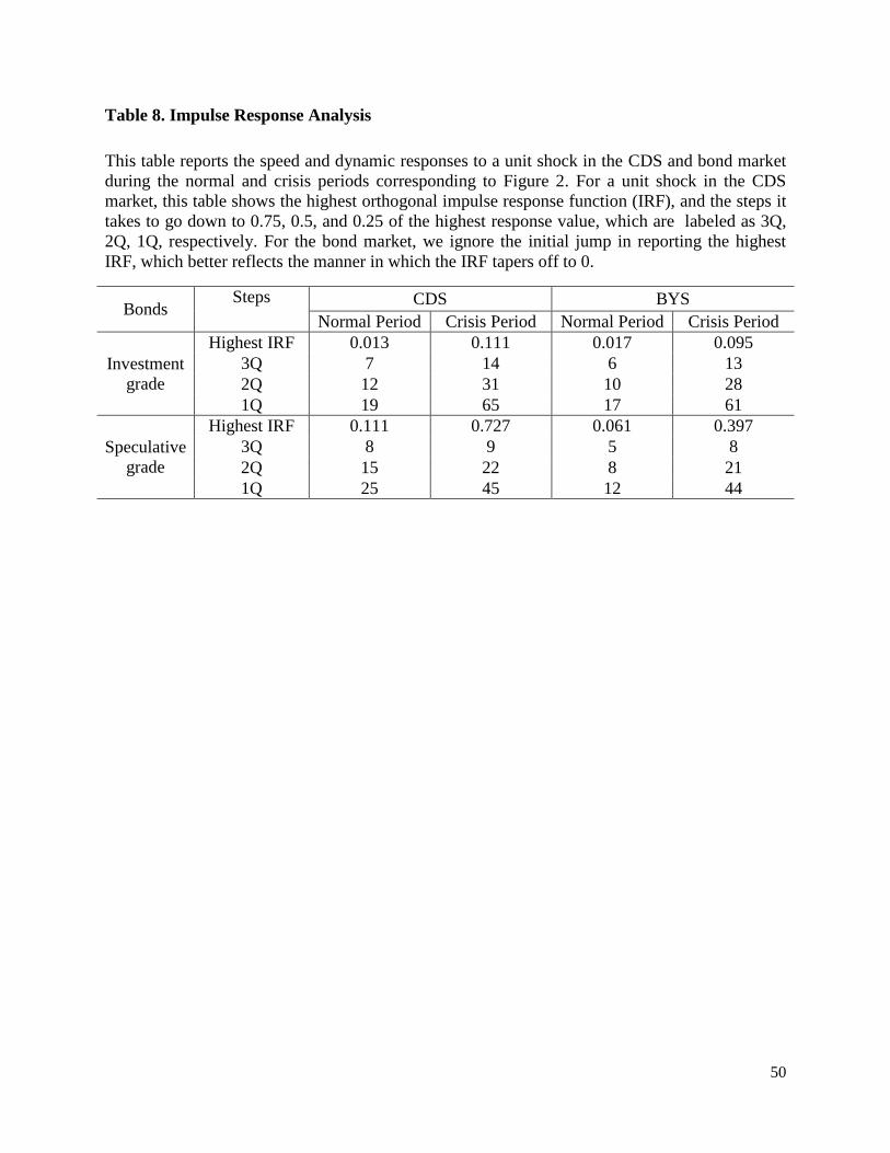
50
Table 8. Impulse Response Analysis
This table reports the speed and dynamic responses to a unit shock in the CDS and bond market
during the normal and crisis periods corresponding to Figure 2. For a unit shock in the CDS
market, this table shows the highest orthogonal impulse response function (IRF), and the steps it
takes to go down to 0.75, 0.5, and 0.25 of the highest response value, which are labeled as 3Q,
2Q, 1Q, respectively. For the bond market, we ignore the initial jump in reporting the highest
IRF, which better reflects the manner in which the IRF tapers off to 0.
Bonds Steps CDS BYS
Normal Period Crisis Period Normal Period Crisis Period
Investment
grade
Highest IRF 0.013 0.111 0.017 0.095
3Q 7 14 6 13
2Q 12 31 10 28
1Q 19 65 17 61
Speculative
grade
Highest IRF 0.111 0.727 0.061 0.397
3Q 8 9 5 8
2Q 15 22 8 21
1Q 25 45 12 44

51
Table 9. Persistence analysis
We report the persistence estimate as measured by the long memory parameter (d) based on the rescaled
range R/S statistic for different bond groups and periods. Estimation is conducted using the daily data and
its time aggregates from 2 to 10 days. Detail estimation method is described in Appendix C. Persistence
analysis is performed on the basis, the absolute basis, and absolute basis changes as a proxy for volatility.
Panel A: Long memory d estimates and two-sample t-tests by bond grade
We test of the null of the same persistence for speculative- and investment-grade (IG) bonds, against a one-
sided alternative hypothesis that the former is more persistent. Estimation is conducted over the whole
sample period. The persistence measure and significance test results (p-values) are reported.
Basis |Basis| Volatility = |∆Basis|
Speculative grade 0.398 0.393 0.235
Investment grade 0.373 0.357 0.183
Difference 0.025 0.036 0.052
p-value 0.035 0.006 0.000
Panel B: Long memory d estimates and two-sample t-tests by subperiod
We test the null of the same persistence during crisis and normal periods, against a one-sided alternative
hypothesis that it is more persistent during crisis. Estimation is conducted over the normal and crisis
periods. The persistence measure and significance test results (p-values) are reported.
Panel C: Long memory d estimates and two-sample t-tests by bond grade and sample period
Investment grade Speculative grade Difference p-value
Basis
Crisis period 0.385 0.400 0.015 0.153
Normal period 0.343 0.357 0.014 0.215
Difference 0.042 0.043
p-value 0.000 0.000
Absolute basis: |Basis|
Crisis period 0.378 0.388 0.010 0.218
Normal period 0.323 0.363 0.040 0.021
Difference 0.055 0.025
p-value 0.000 0.021
Absolute basis changes: |∆Basis|
Crisis period 0.202 0.225 0.023 0.087
Normal period 0.143 0.205 0.061 0.000
Difference 0.058 0.020
p-value 0.000 0.075
Basis |Basis| Volatility = |∆Basis|
Crisis period 0.390 0.381 0.210
Normal period 0.347 0.336 0.164
Difference 0.043 0.045 0.046
p-value 0.000 0.000 0.000

52
Table 10. Persistence Analysis with Long Memory FIGARCH Model
This table reports the MA(1)-FIGARCH(1,1) estimation result for Basis of investment-grade
(IG) bonds and speculative-grade (SG) bonds over the normal and crisis periods. The normal
period is from January 2005 to June 2007 and the crisis period is from July 2007 to December
2009. P-value is given in parentheses. The model is: 11 ttt eecbasis where
2
1 1 0 1(1 ( ) )(1 ) (1 )d
t tB B e B v with 22
ttt ev .
Bonds Period c 1 0
1 1 d
Investment
grade
Normal 0.000 -0.762 0.000 0.774 0.694 0.121
(0.493) (0.000) (0.123) (0.000) (0.000) (0.087)
Crisis 0.001 -0.529 0.000 0.830 0.396 0.740
(0.236) (0.000) (0.036) (0.000) (0.000) (0.000)
Speculative
grade
Normal 0.000 -0.725 0.004 0.474 0.369 0.131
(0.399) (0.000) (0.188) (0.106) (0.150) (0.099)
Crisis 0.006 -0.617 0.007 0.784 -0.074 0.974
(0.154) (0.006) (0.000) (0.000) (0.246) (0.000)