Learning-based super resolution using kernel partial least squares

Image and Vision Computing 29 (2011) 394–406

Contents lists available at ScienceDirect

Image and Vision Computing

j ourna l homepage: www.e lsev ie r.com/ locate / imav is

Learning-based super resolution using kernel partial least squares☆

Wei Wu a, Zheng Liu b,⁎, Xiaohai He a

a School of Electronics and information Engineering, Sichuan University, Chengdu, 610064, Chinab School of Information Technology and Engineering, University of Ottawa, Ottawa, ON, Canada K1N 6N5

☆ The paper has been recommended for acceptance b⁎ Corresponding author. Tel.: +1 613 9933806; fax: +

E-mail address: [email protected] (Z. Liu).

0262-8856/$ – see front matter. Crown Copyright © 20doi:10.1016/j.imavis.2011.02.001

a b s t r a c t
a r t i c l e i n f o
Article history:Received 11 January 2010Received in revised form 14 October 2010Accepted 6 February 2011

Keywords:Learning-based super resolutionHigh resolution imageKernel partial least squaresResidual image

In this paper, we propose a learning-based super resolution approach consisting of two steps. The first stepuses the kernel partial least squares (KPLS) method to implement the regression between the low-resolution(LR) and high-resolution (HR) images in the training set. With the built KPLS regression model, a primitivesuper-resolved image can be obtained. However, this primitive HR image loses some detailed information anddoes not guarantee the compatibility with the LR one. Therefore, the second step compensates the primitiveHR image with a residual HR image, which is the subtraction of the original and primitive HR images.Similarly, the residual LR image is obtained from the down-sampled version of the primitive HR and originalLR image. The relation of the residual LR and HR images is again modeled with KPLS. Integration of theprimitive and the residual HR image will achieve the final super-resolved image. The experiments with face,vehicle plate, and natural scene images demonstrate the effectiveness of the proposed approach in terms ofvisual quality and selected image quality metrics.

Crown Copyright © 2011 Published by Elsevier B.V. All rights reserved.

1. Introduction

In the applications of surveillance, object tracking, and vehiclelicense plate recognition, the acquired images are usually of lowresolution, which may result in a failure of further analyses such assegmentation and recognition. Deriving a high-resolution (HR) imagefrom the low-resolution (LR) one or a sequence of LR images providesa solution to these applications, which is known as the superresolution (SR) imaging technique [3,17,25]. The derived high-resolution image is also called super-resolved image. Generally, theSR algorithms can be categorized into two classes, i.e. multi-framebased approach [7,10,18] and single-frame based approach, which isalso called learning-based approach [1,5,13,14,29]. In the multi-framebased approach, the HR image is derived from several LR observationsof the scene, which are typically aligned with sub-pixel accuracy;while in the learning-based approach an image database, whichincludes LR and HR image pairs, is used to infer the HR image from itscorresponding LR input. The basic idea of learning-based approach isto model the relation between LR and HR images with the availableimage pairs in the database and then infer HR image from input LRimage with the established model. Compared with the multi-framebased approach, which basically processes images at the signal level,the learning-based approach incorporates more prior information toinfer the unknown HR image. There are basically three types ofimplementations for the learning-based SR algorithm: classification-

y Seong-Whan Lee.1 613 9931866.

11 Published by Elsevier B.V. All rig

based method, reconstruction-based method, and regression-basedmethod. Figs. 1–3 illustrate these methods. To facilitate the proces-sing, the images are usually represented by patches, which could be apixel, an image block, or even an image.

Classification-based method is to find the similar image patchesfrom the training set for the input LR patches through a classificationprocess (see Fig. 1). The super-resolved image patches are inferredfrom its LR inputs with an inferencemethod, such as Markov network,and then these HR patches are integrated into a full HR image. In thismethod, features need to be identified and extracted. Varied multi-resolution approaches including Gaussian pyramid, Laplacian pyra-mid, steerable pyramid, wavelets, and contourlet have been proposedto extract image features in an SR application. Freeman et al. proposeda sample-basedmethod in [6]. A Markov networkwas trained to learnthe relationship between the LR images and their corresponding HRimages. The trained Markov network was used to infer an HR imagefrom its input LR image. Baker and Kanade developed an approachbased on a Gaussian pyramid and Laplacian pyramid model andemployed the Bayesian theory to infer the super-resolved face imagefrom the LR one [1]. Su et al. used a steerable pyramid to extract multi-orientation and multi-scale information of low-level features fromboth the input LR face images and HR face images in database [23]. Apyramidal parent structure and a local best match were adopted tooptimize the prior for solving a Bayesian maximum a posteriori (MAP)problem. Jiji and Chaudhuri proposed a restoration technique usingwavelets, whose coefficients at finer scales of the super-resolvedimage were derived from a set of HR training images [8]. Aregularization was further applied to improve the quality of thefinal super-resolved image. The authors also suggested using the

hts reserved.

http://dx.doi.org/10.1016/j.imavis.2011.02.001

mailto:[email protected]

http://dx.doi.org/10.1016/j.imavis.2011.02.001

http://www.sciencedirect.com/science/journal/02628856

Classification& Match

Training set

... ... ... ...

LR images

... ... ...

HR images

Inferring

...

LRinput

Dividing intopatches

HR output

Integrating

Fig. 1. The implementations of learning-based SR algorithm: the classification-based method.

LRInput

Reconstruction

Training set

LR images

HR images

OutputHR

image

Reconstruction

1C

nC

1C

nC

Fig. 2. The implementations of learning-based SR algorithm: the reconstruction-based method.

395W. Wu et al. / Image and Vision Computing 29 (2011) 394–406

contourlet transform [9]. The contourlet coefficients at finer scales forthe input were learnt from a set of HR training images, and the inversecontourlet transform obtained the super-resolved image. The majordisadvantage of the classification-based method is that it needs aclassification algorithm to find the most similar patches for the LRinput patches from the training set. This will inevitably introducequantitative errors. To solve this problem, many approaches intrin-sically rely on a complicated statistical model, which often needs an

Training set

...

... ...

LR images

... ...

HR images

Regression mod

LRinput

Dividinginto patches

Fig. 3. The implementations of learning-based S

explicit resolution reduction function. However, such function issometimes difficult to obtain in practice.

As illustrated in Fig. 2, the reconstruction-based method firstprocesses the training set with principal component analysis (PCA) ora similar method. Thus, the input LR image can be represented withthe principal components from the LR images in the training set. Withthe derived coefficients C1,C2,⋯,Cn, the super-resolved image can beobtained with corresponding components from the HR images in the

...

...

els...

Output HR image

HR output

Integrating

R algorithm: the regression-based method.

Table 1The implementation details of PLS and KPLS algorithms.

Steps PLS KPLS

1 i=1 i=12 Randomly initialize vector ui Randomly initialize vector ui

3 wi=XiTui/ ‖Xi

Tui‖ wi=ΦiTui/ ‖Φi

Tui‖

ti=Xiwi

ti = Φiwi = ΦiΦTi ui = uT

i ΦiΦTi ui

� �12

= Kiui =ffiffiffiffiffiffiffiffiffiffiffiffiffiffiffiuTi Kiui

q

4 ci=YiTti/tiTti ci=Yi

Tti/tiTti5 ui=Yici/ciTci ui=Yici/ciTci6 Repeat steps 3–5 until ui converges to obtain ui, ti, and wi, ci Repeat steps 3–5 until ui converges to obtain ui, ti, and wi, ci7 Deflate Xi, Yi:

Xi=Xi−titiTXi/tiTtiDeflate Ki, Yi:Ki=(I−titiT/tiTti)Ki(I−titiT/tiTti)

Yi=Yi− titiTYi/tiTti Yi=Yi− titiTYi/tiTti8 i= i+1,goto step 2 i= i+1,goto step 2

396 W. Wu et al. / Image and Vision Computing 29 (2011) 394–406

training set. Following this procedure, Wang and Tang used PCA to fitthe input face image as a linear combination of the LR facecomponents in the training set [26]. Then, the super-resolved imagewas rendered by replacing the LR components in the training set withtheir corresponding HR ones, while retaining the same combinationcoefficients. Reconstruction-based method provides a better way todeal with quantitative error. However, PCA is a linear transformation,which may cause the overfitting problem during the training processand may lead to a poor result as well.

Different from the aforementioned methods, regression-basedmethod firstly builds a regression model according to the relation ofLR image patches and HR image patches (see Fig. 3). The regression

Fig. 4. The flowchart of the proposed approach: (1) feeding the input image to the built KPLS(3)down-sampling the primitive HR image; (4) obtaining the difference image between the dthe KPLS regression model at step two; (6) inferring the residual HR image; (7) integratingapproach: (8) building the KPLS model for LR and HR images in the training set; (12) buildin(10) down-sampling primitive HR image; and (11) obtaining residual LR images.

model is then used to infer super-resolved image patches from the LRinputs. Quantitative errors can be compensated to some extent withthe regression-based method. One typical regression-based method isdescribed in Ref. [15], where support vector regression (SVR) wasused to build a relationship between known LR and unknown HRpatches. Due to the strong correlation of adjacent pixels in an image,the regression in super resolution becomes a multiple outputproblem. However, this method treats the multi-output regressionproblem as a multiply separated single-output regression problem,which ignores the correlation of different outputs; specifically, thecorrelation between adjacent pixels is ignored. Besides, there arequite a number of parameters that need to be tuned in the SVR

regression model at step one; (2) inferring the primitive HR image by using single KPLS;own-sampled primitive HR image and input LR image; (5) feeding the residual image tothe primitive HR image the residual HR image. There are two training processes in theg the KPLS model for residual LR and HR images: (9) obtaining the residual HR images;

Fig. 5. An example of face image for feature extraction (↑: up-sampling operation): (a)HR image Ih(x,y); (b) enlarged LR image ↑ Il(x,y); (c) difference Ih(x,y)−↑ Il(x,y); and(d)DoG feature map.


method. In addition, the inferred results cannot guarantee thecompatibility with the LR one.

Other solutions combining two or three aforementioned methodsare also available for the SR problem. One example combining globaland local models was given by Liu et al. in Ref. [13]. The authors usedthe construction-based method to derive a global linear model andthe classification-based method to capture the high-frequencycontents with a non-parametric Markov network. By integrating theglobal and the local models, photorealistic face images were achieved.

Fig. 6. The use of different features: first row is the result of using luminance values;second row is the result of using the DoG feature. The right side of each row is thezoomed version of the marked region on the left side.

However, the effectiveness of such a combinational method relied onthe successes of both models.

This paper presents a learning-based super resolution algorithmusing kernel partial least squares (KPLS) regression. The KPLSalgorithm is capable of dealing with the nonlinear problem andthere are fewer parameters needed to be adjusted in the implemen-tation in comparison to the SVR method. The relevance of adjacentpixels is preserved during the process. A two-step procedure for KPLS-based super resolution is proposed. The relation between HR outputand LR input images is first modeled with the KPLS algorithm, wherethe features, i.e. mid-frequency information from the LR image, are fedinto the KPLSmodel and high-frequency information for the HR imagecan be derived. A similar process is applied to the residual LR and HRimages, which enables compensation to the HR image. Thus, a furtherimprovement of the quality of the super-resolved image is possible.

The rest of this paper is organized as follows. In Section 2, theprinciple of KPLS is briefly described. This section also presents a two-step procedure to implement the KPLS-based super resolution.Experimental results with face, vehicle plate, and natural sceneimages can be found in Section 3. This paper is summarized inSection 4.

2. Super resolution with kernel partial least squares regression

A low-resolution image can be produced from a high-resolutionimage by a down-sampling operation. This process can bemodeled as:

Il x; yð Þ = ↓ Ih x; yð Þ � h x; yð Þ½ � ð1Þ

where Il(x,y) and Ih(x,y) are the LR and HR images respectively. h(x,y)is the point spread function of the imaging system. ↓ refers to thedown-sampling operation. Super resolution is an inversion of theabove process, i.e. obtaining the high-resolution image Ih(x,y) fromthe given degraded LR image Il(x,y). The super resolution problemremains ill-posed, since there are many Ih(x,y) satisfying Eq. (1) givena Il(x,y). In this paper, the kernel partial least squares regression isemployed to implement the super resolution process.

2.1. Partial least squares and kernel partial least squares

2.1.1. Partial least squares (PLS)Partial least squares (PLS) method is a multivariate projection

method, which has been applied to a wide range of regressionapplications. It models the relationship between a set of inputvariables x∈RN and a set of output responses y∈RM [19]. Supposethat a (n×N) matrix of zero-mean variables X consists of the rowscreated by n N-dimensional inputs x and the (n×M) matrix ofcorresponding responses Y consists of the rows created by n M-dimensional outputs y. The PLS regression model can be expressed as:

Y = XB + Z ð2Þ

where B is a matrix (N×M) with regression coefficients and Z is aresidual matrix (n×M). To calculate regression coefficients B, PLSdecomposes X and Y into the form:

X = TPT + E ð3Þ

Y = UQ T + F ð4Þ

where T; U are the score matrices (n×d) whose columns consist of dextracted score vectors ti and ui, i=1,2,…,d respectively, while P; Q ,determining the linear combination of the inputs and outputs, are theloading matrices of size (N×d) and (M×d) respectively. And P; Qconsist of the columns created by the d load vectors pi and qi

image of Fig.�5

image of Fig.�6

Fig. 7. The procedure for estimating a primitive HR image.


respectively. The (n×N) matrix E and (n×M) matrix F represent theresidual matrices.

The standard algorithm for computing partial least regressioncomponents is the nonlinear iterative partial least squares (NIPALS),which calculates the components sequentially rather than calculatesall the components at one time, i.e. the score vectors ti and ui, and theweight vectors wi and ci, i=1,2,…,d are sequentially extracted fromthe input variablesX and output responses Y. Theweight vectorswi, cias well as score vectors ti and ui satisfy Ref. [19]:

cov ti;uið Þ½ �2 = cov Xwi;Ycið Þ½ �2 = maxrj j= sj j=1

cov Xr;Ysð Þ½ �2

= maxrj j= sj j=1

var Xrð Þ corr Xr;Ysð Þ½ �2var Ysð Þn o ð5Þ

where cov, var, and corr denote the sample covariance, variance, andsquared correlation respectively. Eq. (5) denotes that PLS algorithmbalances with the requirement to explain as much variance aspossible in both X and Y by using the criterion of maximal correlation[19]. On obtaining the score vectors ti and ui, X and Y are deflated bysubtracting the rank-one approximations based on ti and ui. The leftcolumn of Table 1 shows the details of PLS algorithm.

At the beginning of the PLS procedure, we set X1 = X and Y1 = Y.The subscript i in the PLS algorithm refers to ith iteration (starting fromstep2, andrepeatingstep3–5untilui converges),wherewecanobtain thescore vectors ui n × 1ð Þ, ti n × 1ð Þ and the weight vectors wi N × 1ð Þ,ci M × 1ð Þ. After the ith iteration, the algorithm starts again from step 2 byusing the deflated matrices Xi and Yi computed in step 7.

The loading vectors pi and qi can be computed as follows:

pi = XTi ti = tTi ti

� �ð6Þ

qi = YTi ui = uT

i ui

� �ð7Þ

Finally, the regression coefficient matrix B in PLS regression modelcan be expressed as [22]:

B = XTU TTXXTU� �−1

TTY ð8Þ

2.1.2. Kernel partial least squares (KPLS)PLS is a linear regression method; however, in many applications

we need to solve a nonlinear problem. Motivated by the recent

research on kernel-based learning, a nonlinear kernel-based PLS wasproposed in Ref. [20] as an extension of PLS.

The key idea of the kernel PLS approach is to map the input data toa high-dimensional feature space F corresponding to a reproducingkernel Hilbert space, where the nonlinear structure in the input spaceis more likely to be linear, and a linear PLS can be applied [12,21].Consider a nonlinear transformation of the input data xi (i=1,⋯,n)into feature space F:

Φ : xi ∈ RN→Φ xið Þ ∈ F ð9Þ

where the mean centering in the high-dimensional space is applied,i.e., ∑n

i=1Φ xið Þ = 0, and Φ xið Þ is the nonlinear mapping functionwhich maps the input data xi from the input space to F. Note that S,the dimensionality of the feature space F, may be arbitrarily large andcan even be infinite. Through the introduction of kernel function,k xi;xj� �

= Φ xið ÞΦT xj� �

, there is no need to perform explicit nonlinearmapping and compute dot products in the feature space [28]. Thekernel function k(⋅) needs to meet the Mercer theorem condition [20]and the widely used kernel functions include radial basis kernel,polynomial kernel, and sigmoid kernel [28]. In this paper, we used theradial basis kernel, k xi;xj

� �= exp − ∥xi−xj∥2 = c

� �� , in our imple-

mentation. The KPLS algorithm, can be directly derived from the PLSalgorithm bymodifying steps 3 and 7 of the PLS procedure so as to usethe mapped input data Φ xið Þ instead of the original input data xi. TheKPLS algorithm is illustrated on the right column of Table 1 [28].

In KPLS algorithm, Φ Xð Þ is a (N×S) matrix with the ith row is thevector Φ xið Þ in the feature space F and K = Φ Xð ÞΦ Xð ÞT is the kernelmatrix. At the beginning of the KPLS procedure, we set K1 = K,Φ1 = Φ Xð Þ, and Y1 = Y.

Similar to PLS algorithm, from the ith iteration of KPLS, we can obtainscore vectors ui, ti,wi, and ci. Rather than using the deflated matrices Xi

and Yi as in PLS, KPLS uses deflated matrices Ki and Yi to start the nextiteration. The regression coefficient matrix B has the form:

B = ΦTU TTKU� �−1

TTY ð10Þ

To make a prediction for the input xt with the trained model, wehave:

Yt = ΦtB = KtU TTKU� �−1

TTY ð11Þ

image of Fig.�7

Fig. 8. The procedure of building regression models: (a) building regression models forspatially variant phenomena (1) building the models, (2) feeding new LR patches intothe models; (b) building regression models for spatially invariant phenomena (1)finding the Nmost similar LR patches in the training set, (2) building themodel, and (3)feeding the LR patch into the model.

1 Herein, mid-frequency information refers to the high-frequency information oflow-resolution image.


whereΦt = Φ xtð Þ is the mapped test data xt . Kt is (1×n) test matrix,whose elements are Kj

t = k xt ; xj� �

; and xj j = 1;2; ⋯;nð Þ are thetraining samples; Yt is the final regression output.

2.2. The two-step implementation

To obtain the super-resolved image, a KPLS regression model S(⋅)is trained by using an image database containing HR images and its LRcounterparts. This process can be modeled as:

Ih x; yð Þ = S Il x; yð Þð Þ ð12Þ

Once the model is built, any input LR image can be processed.However, the model is not “perfect” and only a primitive HR image,Ic(x,y), is obtained:

Ih x; yð Þ ≈ Ic x; yð Þ = S Il x; yð Þð Þ ð13Þ

Some detailed information is missing in the primitive HR image,and the primitive HR image may not satisfy the reconstructionconstraint in Eq. (1). The difference in Eq. (1), i.e. the differencebetween down-sampled version of the primitive HR image and inputLR image, is used to build the second regression model. With thisregression model, the difference is used to estimate the residual HRimage, which compensates the primitive HR image. Specifically, theresidual HR and LR images are first modeled with KPLS algorithmwithin the database. Then, the residual HR image is inferred from itsLR residual. Integrating this residual and primitive HR image cangenerate the super-resolved image for the LR input. The overallprocedure is illustrated in Fig. 4. Details are described below.

2.2.1. Step one: estimation of primitive HR imageThe first issue in super resolution is the representation of image

features. A straightforward way is to define the feature vector as theconcatenation of the luminance values of the pixels in thecorresponding patches from LR or HR images. However, this simplescheme does not assure a good result due to two reasons. First, theluminance values may vary from the lighting conditions. Second, thelow-frequency information from LR image is not as useful as thosefrom its high-frequency band. In other words, the highest frequencyband is conditionally independent of the low-frequency band, whichis expressed as [6]:

P H jM; Lð Þ = P H jMð Þ ð14Þ

where H denotes the high-frequency band information. M and Ldenote the mid- and low-frequency band information respectively.Therefore, the super resolution problem becomes to infer the high-frequency information given the mid-frequency information (fea-tures) from an LR image.

To extract the image feature map or mid-frequency information,1

the LR image is first enlarged and then filtered with a difference ofGaussian (DoG) filter. An example is given in Fig. 5. The DoG featuremap (Fig. 5(d)) is used as the input to the regression model. Thedifference between the HR image and the enlarged LR image (Fig. 5(c))is the corresponding target output. The example in Fig. 6 shows theresults of using luminance values and the DoG features as the inputrespectively.We can see that the result from the luminance values has ablurred edge while the result from the DoG feature map presents moredetails.

To establish an efficient regression model, we divide the imagesinto a set of small patches. However, this may introduce obviousseams between patches. We constrain adjacent patches in an imagethrough overlapping to ensure local compatibility and smoothness.

The detailed procedure for estimating the primitive HR image isgiven in Fig. 7. The procedure comprises of training (Fig. 7 bottom)and estimating processes (Fig. 7 top). The training process goesthrough steps 1 to 6 (Fig. 7 bottom):

1. Each LR image in the training set is enlarged to the same size of itscorresponding HR images with the nearest neighbor interpolation;

2. The DoG filter is applied to the interpolated image to extract thefeature map or mid-frequency information;

3. The DoG feature map is further divided into overlapping patchesconsisting of (m×m) pixels (for example, m=6);

4. The difference between the HR image and the enlarged LR image isobtained;

5. The difference image is also divided into patches;6. The KPLS regressionmodel is built for the patches obtained in 3 and

5 respectively.

image of Fig.�8

Fig. 9. Experimental results with face images.

Table 2Performance assessment of face images.

Method PSNR (dB) SSIM

Nearest neighbor interpolation 29.48 0.811Cubic B-spline interpolation 29.36 0.842Baker's method 29.17 0.781SVR-based method 30.33 0.835Single-step KPLS method (without compensation) 31.65 0.838Proposed method 32.73 0.871


It should be noted that we can also enlarge the LR image by usingcubic B-spline interpolation or filling in zeros and low-pass filtering instep 1. Since the nearest neighbor interpolation is one of the simplestinterpolation methods, we use it rather than other interpolationmethods.

The estimating process repeats steps 1–3 for an input image. Then,the divided patches are fed into the regression model built in thetraining process (step 7). The output patches are reunited into a high-frequency image in step 8. Since the output patches are overlappedwith each other, we use the average of the intensity value for thesuperposed pixels when the patches are integrated into an image.Integrating with the low-frequency image, the HR image is obtainedin the final step 9.

Actually, the images can be classified into two different types [1].One is the spatially variant phenomena; the other is the spatiallyinvariant phenomena. An example of the spatially variant phenomenais frontal face images, where human's nose, mouth, and eyes are atfixed locations on the face. Depending on the spatial location, eachpixel or patch in an input face image is treated differently. However,for text or natural scene images, each pixel or patch is treated in thesame way in spite of its spatial location, and this is known as spatiallyinvariant phenomena. This can be further illustrated with Fig. 8.

To build the regression model for spatially variant phenomena,patches at different locations may need different models. Withmultiple models, the estimation becomes more accurate. The imagepatches in step 3 and step 5 can be denoted as a vector Bi;j;k

L and Bi;j;kH ,

(i=1,⋯,R, j=1,⋯,C) respectively, where (i, j) determines the locationof the patch while k (k=1,⋯,n) refers to the index of images in thetraining set. At each location (i, j), its total n patch/vector pairs, i.e. LRvectors Bi;j;k

L and HR vectors Bi;j;kH in the training set constitute matrices

for the low-resolution inputs and the high-resolution outputsrespectively. The regression model at (i, j) is then built throughthese inputs and outputs. This process can be applied to the faceimage. Fig. 8(a) shows the procedure of building regression modelsfor spatially variant phenomena.

For vehicle plate and natural scene images, which are consideredas spatially invariant phenomena, the regression model is built for allpatches regardless of its location (see Fig. 8(b)). However, the numberof patches in the training is too large. The number of rows andcolumns of the kernel matrix are determined by the product of thenumber of training images and the patches contained in each image.For instance, if we have 100 images in the training set and each imagehas (20×20=400) patches, the square kernel matrix would have(100×20×20=40,000) rows and columns. This becomes a heavyload for computing. To solve this problem, we search the first n LRpatches in the training set with the Euclidean distance measurementthat resemble the input LR image patch most. Then, the n LR patchesare modeled with its corresponding n HR patches. Following the

image of Fig.�9

Fig. 10. Experiments with a photograph.

30

31

32

33

34

1 2 3 4 5 6 7 8 9 10 11 12 13 14 15 16 17 18 19 20 21 22

Number of KPLS components

PSN

R(d

B)

Proposed method

Single-step KPLS method

Fig. 11. The impact of the number of KPLS components and the second step for faceimages.


procedure in Fig. 8, themodels for the face images and vehicle plate ornatural scene images can be built respectively.

The first three steps of the super-resolution learning process aresimilar to those of the training process. The input LR image isrepresented by divided patches BL;input

i;jð Þ . And the patches are fed to the

Fig. 12. The impact of patch size for face images.

image of Fig.�10

image of Fig.�11

30.5

31

31.5

32

32.5

33

33.5

34

37 47 57 67

Number of patch pairs

PSN

R(d

B)

Proposed method


Fig. 13. The impact of the number of patch pairs used to build regressionmodels for faceimages.

Table 3Performance assessment for vehicle plate images.




model built at the training stage. The output patches BH;outputi;jð Þ are

reunited into a high-frequency image. By integrating the high-frequency image with the enlarged LR image, a primitive high-resolution image is obtained. As aforementioned, some detailedinformation is missing in the first step. A compensation step issuggested as follows.

2.2.2. Step two: compensation with the residual imageThe single KPLS process generates a primitive HR image, which

looks smooth but may lose some detailed information. Thus, Ic(x,y) isdifferent from Ih(x,y) and the difference, i.e. IhR= Ih(x,y)− Ic(x,y) is theresidual HR image. Similarly, the residual LR image Il

R(x,y) is defined

Fig. 14. Experimental results with vehicle plate images.

as the difference between Il(x,y) and the down-sampled version of thecorresponding primitive HR image, i.e. IlR(x,y)= Il(x,y)−↓ Ic(x,y).

The problem now becomes inferring IhR(x,y) given IlR(x,y). Once IhR(x,y)

is available, Ih(x,y) can be easily obtained by Ih(x,y)= IhR(x,y)+ Ic(x,y).

Similar to step one, the relation between IhR(x,y) and Il

R(x,y) can bemodeled as:

IRH x; yð Þ = Q IRl x; yð Þ� �

ð15Þ

Herein, KPLS is again applied to estimate the nonlinear mappingQ(⋅). As described in thefirst step, the regressionmodel can be built andapplied.When the residual HR image is estimated from the secondKPLSmodel, the addition of the results from the two steps gives the finalsuper-resolved image.

3. Experimental results

The experiments consist of three parts. First experiment is withface images. The second one uses vehicle plate images. The thirdexperiment deals with natural scene images. In the experiments, weconsidered other four methods for comparison: nearest neighbor,cubic B-spline interpolation, Baker's method, and support vectormachine (SVR) based method.

In the experiment, the size of the patches is set as 6×6 and theneighbor patches are overlapped by two pixels. The number of KPLScomponents for face is eight, and the number of KPLS components forvehicle plate and natural scene images is ten. For face images, thespatially variant phenomena, the regression model at location (i, j) isbuilt by 67 LR and HR patch pairs selected from the same location ofthe training images. For plate and natural scene images, the spatiallyinvariant phenomena, seven hundred LR patches, which resemble theinput LR image patches most, are selected from the training settogether with their corresponding HR patches to build the regressionmodels.

To quantify the improved performance in the experiment, LRtesting images for face, vehicle plate, and natural scene are generatedby low-pass filtering and down-sampling HR images. The separablelow-pass filter used in the experiment is [1 4 6 4 1]/16, which isapplied to the HR images in each direction. We employed peak signal-to-noise ratio (PSNR) and the structural similarity measurement(SSIM) as metrics to evaluate the obtained super-resolved image [27].The mean value of all the test images' PSNR and SSIM is used as ametric. The SSIMmetric needs a “perfect” reference image to compare

Table 4Character recognition assessment for characters in vehicle plate images.

Method Recognition accuracy

Nearest neighbor interpolation 80.00%Cubic B-spline interpolation 90.51%Baker's method 88.48%SVR-based method 87.47%Single-step KPLS method(without compensation) 94.34%Proposed method 94.95%Original image 97.37%

image of Fig.�13

17

18

19

20

21

22

23

24

1 2 3 4 5 6 7 8 9 10 11 12 13 14 15 16 17 18 19 20 21 22


PSN

R(d

B)

Proposed method


Fig. 15. The impact of the number of KPLS components and residual compensation forvehicle plate images.

Fig. 16. The impact of patch size for vehicle plate images.

20

20.5

21

21.5

22

22.5

23

100 300 500 700


PSN

R(d

B)

Proposed method


Fig. 17. The impact of the number of patch pairs for vehicle plate images.

Fig. 18. Some examples of


and gives a normalized value between [0,1], where “0” indicates thatthe two images are totally different while “1” confirms that the twoimages are the same. Thus, the higher values these two metrics are,the better quality the result is.

3.1. Experiments with face images

The face images used in this experiment were obtained from theAsian face image database [4]. The database contains 107 persons,among whom 51 are females and 56 are males. Each person has 17different images: one frontal face, four illumination variations, eightpose variation, and four expression variations. Twenty-four males andeight females wear glasses. Most of the volunteers are between theages 20 and 30. We selected 75 persons with no glasses from the 107.The training set randomly selected 67 from the 75 persons and the rest8 persons' images were used as inputs for testing. All the images,normalized to size 192×160 are considered as HR images. The 67 hrtraining images were down sampled to get its LR images of size 48×40.

An example of the super-resolved images is given in Fig. 9. Fourface images are presented from left to right. Fig. 9(a) shows the“perfect” references. Other images were obtained with differentalgorithms. It is found that the edges are better preserved in thesuper-resolved images in Fig. 9(d)–(g) while the nearest neighborand cubic B-spline interpolation blur most of the images' details inFig. 9(b) and (c). Fig. 9(d) obtained with Baker's method presentssignificant noises and artifacts. The results of SVR-based methodwhich show in Fig. 9(e) have moderate artifacts compared with theBaker's method. There is no obvious artifact available in the resultsobtained with the proposedmethod (see Fig. 9(f)). In comparison, theSVR-based method presents more noises for local face features, suchas face contour, nostril, and eyebrow.

In terms of the metric values in Table 2, the proposed methodachieved the best results. It achieved up to three dB gain in PSNR overthe cubic B-spline interpolation and two dB gain over the SVR-basedmethod.

Second example is a photograph containing an LR face in Fig. 10(a),which is obtained from a camera rather than from a down-sampledversion of HR image. We applied the proposed algorithm to theextracted region of the face image. Results are given in Fig. 10(b). Aswe do not have the “truth” HR image, the quantitative assessment isnot available for this test, but the results can still be evaluatedsubjectively. We can see that the results of the proposed approach iswith more high-frequency details and better than the results of othermethods.

natural scene images.

image of Fig.�15

image of Fig.�17

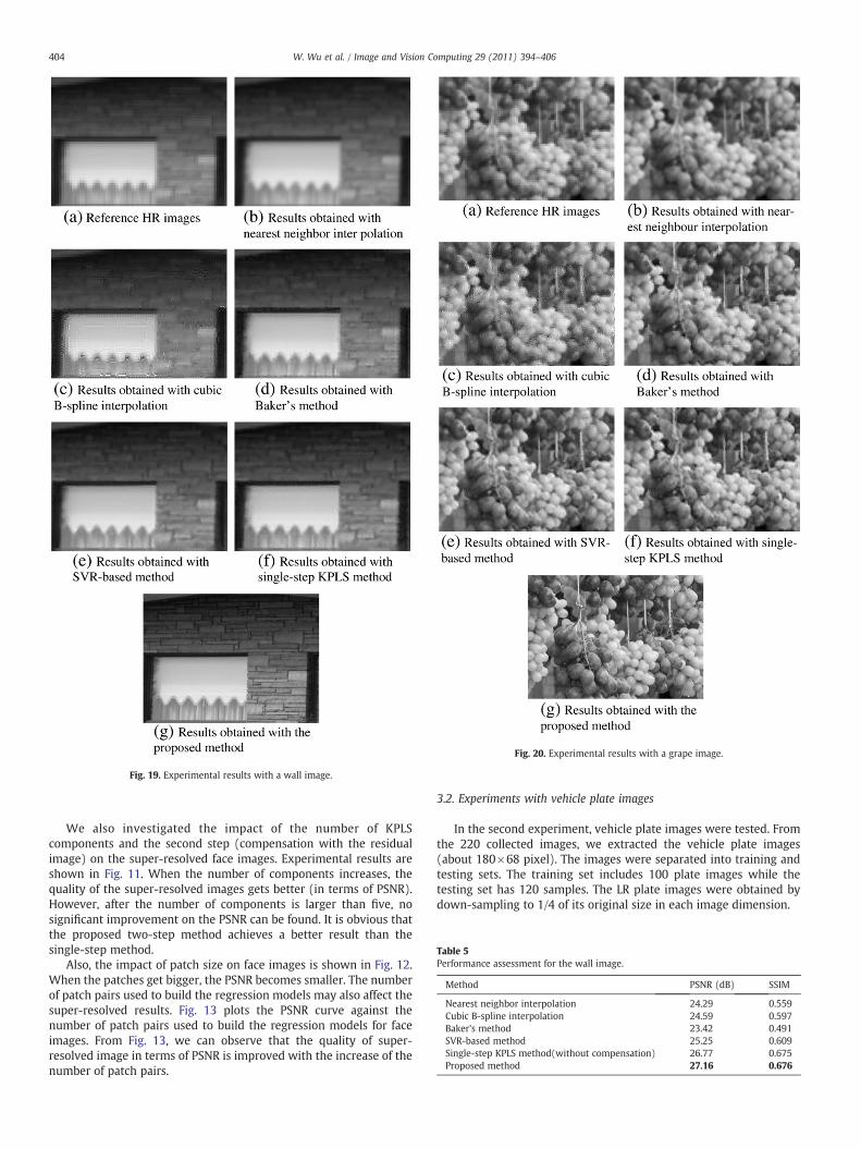
Fig. 19. Experimental results with a wall image.

Fig. 20. Experimental results with a grape image.

Table 5Performance assessment for the wall image.


Nearest neighbor interpolation 24.29 0.559Cubic B-spline interpolation 24.59 0.597Baker's method 23.42 0.491SVR-based method 25.25 0.609Single-step KPLS method(without compensation) 26.77 0.675Proposed method 27.16 0.676


We also investigated the impact of the number of KPLScomponents and the second step (compensation with the residualimage) on the super-resolved face images. Experimental results areshown in Fig. 11. When the number of components increases, thequality of the super-resolved images gets better (in terms of PSNR).However, after the number of components is larger than five, nosignificant improvement on the PSNR can be found. It is obvious thatthe proposed two-step method achieves a better result than thesingle-step method.

Also, the impact of patch size on face images is shown in Fig. 12.When the patches get bigger, the PSNR becomes smaller. The numberof patch pairs used to build the regression models may also affect thesuper-resolved results. Fig. 13 plots the PSNR curve against thenumber of patch pairs used to build the regression models for faceimages. From Fig. 13, we can observe that the quality of super-resolved image in terms of PSNR is improved with the increase of thenumber of patch pairs.

3.2. Experiments with vehicle plate images

In the second experiment, vehicle plate images were tested. Fromthe 220 collected images, we extracted the vehicle plate images(about 180×68 pixel). The images were separated into training andtesting sets. The training set includes 100 plate images while thetesting set has 120 samples. The LR plate images were obtained bydown-sampling to 1/4 of its original size in each image dimension.

image of Fig.�19

image of Fig.�20

Table 6Performance assessment for the grape image.



Fig. 22. The impact of patch size for natural scene images.


Fig. 14 shows the results of the corresponding experimentsconducted on the low-resolution plate images. The super-resolvedimages obtained by the proposed approach are much sharper thanthose obtained by the interpolation methods. In particular, the edgesare better preserved in the super-resolved image using our method.The results of the Baker's method present lots of noise, while theresults of the SVR-based method demonstrate a slight improvement.

The proposed method gives the clearest images. All the charactersin the plate can be easily identified. Since plate images have morehigh-frequency information, the improvement of plate images is moreobvious than that of face images. Again, the objective assessment isavailable in Table 3, fromwhich we can see that the proposed methodachieved the best.

To further understand the performance on vehicle plate images,we adopt a goal-directed evaluation to assess the super-resolvedimage through character recognition [24]. Since each plate image has6 numeric and alphabetic characters, totally we can get (120×6)characters. Each segmented character is then normalized to a size(33×17) with a bilinear interpolation method. Then, Ostu's method isapplied to binarize each character [16]. The characters are furtherdivided into five groups. Each group is used as the templates in turnand the remaining four groups are used for testing. The finalrecognition rate is obtained by averaging the five test results.Recognition is performed by comparing an input character with thetemplates. The comparison uses the normalized cross-correlationbetween the input character and the templates [2]. With a completecomparison, the character is identified as the most similar template,which has the maximum normalized cross-correlation. The recogni-tion accuracy for different methods is given in Table 4. The proposedmethod achieved a higher accuracy rate when compared with theothers.

The changes of PSNR are plotted against the number of KPLScomponent for vehicle plate images in Fig. 15. Similarly, the quality ofa super-resolved image is improved with the increase of the numberof components. When the number goes beyond eight, no significantimprovement is observed. Also, the proposed two-step methodoutperforms the single-step one.

The plot of PSNR against patch size for vehicle plate images is givenin Fig. 16. Different from the face images, there is no clear relationshipbetween the PSNR value and the patch size.

23

24

25

26

27

1 2 3 4 5 6 7 8 9 10 11 12 13 14 15 16 17 18 19 20 21 22


PSN

R(d

B)

Proposed method


Fig. 21. The impact of the number of KPLS components and residual compensation fornatural scene images.

Finally, we investigated how the number of patch pairs used tobuild the regression models might affect the final results. Fig. 17 plotsthe PSNR curve against the number of patch pairs. When the numberof patch pairs is beyond 500, no obvious improvement for both single-step KPLS method and the proposed method is achieved.

3.3. Experiments with nature scene images

Experiments are also performed on natural scene images. Thetraining set consists of 80 images of different types of objects such asplants, buildings, and animals. Fig. 18 shows some examples of naturalscene images used in these experiments. Figs. 19(a) and 20(a) showtwo sample HR images, a wall image and a grape image, which aredown-sampled by factor 4 to get the corresponding LR images fortesting. Figs. 19(b)–(g) and 20(b)–(g) show the experimental resultsconducted on the low-resolution images. We can observe a similarperformance as observed in the experiments for vehicle plate images.The objective assessments are listed in Tables 5 and 6, from which wecan see that the proposed method achieves the best results.

The changes of PSNR (mean value of PSNR of the wall and grapeimages) are plotted against the number of KPLS component fornatural scene images in Fig. 21. The impact of the KPLS component fornatural scene images is similar to that of face and vehicle plate images.

The plot of PSNR against patch size for natural scene images isgiven in Fig. 22. Fig. 23 shows how the number of patch pairs used tobuild regression models may affect the super-resolved results fornatural scene images. Similar to vehicle plate images, there is no clearrelationship between the PSNR value and the patch size. When thenumber of patch pairs is beyond 500, no obvious improvement for theproposed method is observed.

4. Summary

In this paper, we propose a learning-based super resolutionalgorithm using kernel partial least squares. The algorithm consists oftwo steps, i.e. estimation of the primitive super-resolved image andcompensation with the residual image. The whole procedure actuallyimplements a dual-learning process. In either case, a training processis carried out to build a regression model with the pairs of inputs andoutputs. The use of KPLS makes it possible to handle multiple outputs

23.5

24

24.5

25

25.5

26

26.5

100 300 500 700


PSN

R(d

B)

Proposed method


Fig. 23. The impact of the number of patch pairs for natural scene images.

image of Fig.�21

image of Fig.�23


without losing the information between adjacent pixels. Theexperimental results with face, vehicle plate, and natural sceneimages demonstrate the effectiveness of the proposed method.

For face, vehicle plate, and natural scene images, the number ofpatch pairs and the number of KPLS components used to build theregression models may have an impact on the super-resolved images.The increase of the number does improve the quality of the super-resolved image in terms of PSNR. However, there is a limitation inboth cases; when the number is beyond a certain threshold value, nosignificant improvement is observed. The proposed two-step methodachieves better super-resolved results than the single-step KPLSmethodwhen they have the same number of components and patchesin the regression models. The patch size may also have an impact onthe super-resolved images. An appropriate size can achieve anoptimal result. However, choosing such a size is still an open issueand remains a topic for our future research [11].

For our future work, the proposed method can be furtherimproved by implementing an iterative process. The step two canbe repeatedly applied to compensative residual images until a certainconvergence condition is met, for instance, ‖Il(x,y)−↓ Ic(x,y)‖b∂,where ∂ is a pre-selected positive constant value. Other possibleimprovements include choosing an appropriate patch size to achieveoptimal performance, finding the suitable patches to build theregression model, and selecting a better one from a bunch ofregression models built in advance.

Acknowledgement

This work is supported by the National Natural Science Foundationof China (project number: 61071161).

References

[1] S. Baker, T. Kanade, Limits on super-resolution and how to break them, IEEETransactions on Pattern Analysis and Machine Intelligence 24 (9) (2002)1167–1183.

[2] K. Briechle, U.D. Hanebeck, Template matching using fast normalized crosscorrelation, In Proceedings of SPIE: Optical Pattern Recognition XII, vol. 4387,March 2001, pp. 95–102.

[3] D. Capel, A. Zisserman, Computer vision applied to super resolution, IEEE SignalProcessing Magazine 20 (3) (2003) 75–86.

[4] H. Dong, N. Gu, Asian face image database PF01, Technical Report, PohangUniversity of Science and Technology, 2001.

[5] W.T. Freeman, T.R. Jones, E.C. Pasztor, Example-based superresolution, IEEEComputer Graphics and Applications 22 (2) (2002) 56–65.

[6] W.T. Freeman, E. Pasztor, O.T. Carmichael, Learning low-level vision, InternationalJournal of Computer Vision 40 (10) (2000) 25–47.

[7] M. Irani, S. Peleg, Improving resolution by image registration, Journal of ComputerVision, Graphics, and Image Processing 53 (3) (1991) 231–239.

[8] C.V. Jiji, S. Chaudhuri, Single frame super-resolution using learned waveletcoefficients, International Journal of Imaging Systems and Technology 14 (3)(2004) 105–112.

[9] C.V. Jiji, S. Chaudhuri, Single-frame images super-resolution through contourletlearning, EURASIP Journal on Applied Signal Processing 2006 (2006) 1–11.

[10] S. Kim, W. Su, Recursive high-resolution reconstruction of blurred multiframeimages, IEEE Transactions on Image Processing 2 (10) (1993) 534–539.

[11] K.V. Kumar, A. Negi, Subxpca and a generalized feature partitioning approach toprincipal component analysis, Pattern Recognition 41 (4) (April 2008)1398–1409.

[12] F. Lindgren, P. Geladi, S. Wold, The kernel algorithm for PLS, Journal ofChemometrics 7 (1993) 45–59.

[13] C. Liu, H.-Y. Shum, W.T. Freeman, Face hallucination: theory and practice,International Journal of Computer Vision 75 (10) (2007) 115–134.

[14] W. Liu, D. Lin, X. Tang, Face hallucination through dual associative learning,Proceedings of IEEE International Conference on Image Processing. Genoa, Italy,20058, pp. I-873-6.

[15] K. Ni, Q.N. Truong, Image superresolution using support vector regression, IEEETransactions on Image Processing 16 (6) (2007) 1596–1610.

[16] N. Otsu, A threshold selection method from gray-level histograms, IEEETransactions on Systems, Man, and Cybernetics 9 (1) (Jan. 1979) 62–66.

[17] S.C. Park, M.K. Park, M.G. Kang, Super-resolution image reconstruction: a technicaloverview, IEEE Signal Processing Magazine 20 (3) (2003) 21–36.

[18] F.-Q. Qin, X.-H. He, W. Wu, Video superresolution reconstruction based onsubpixel registration and iterative back projection, Journal of Electronic Imaging18 (December 2009) 1–16.

[19] R. Roman, K. Nicole, Overview and recent advances in partial least squares,Lecture Notes in Computer Science (2006) 34–51.

[20] R. Roman, L.J. Trejo, Kernel partial least squares regression in reproducing kernelHilbert space, Journal of Machine Learning Research 2 (6) (2001) 97–123.

[21] R. Rosipal, Kernel partial least squares for nonlinear regression and discrimina-tion, Neural Network World 13 (3) (2003) 1–11.

[22] R. Rosipal, N. Kramer, Overview and recent advances in partial least squares, in: C.Saunders, M. Grobelnik, S. Gunn, J. Shawe-Taylor (Eds.), Subspace, LatentStructure and Feature Selection Techniques, Lecture Notes in Computer Science,Springer, 2006, pp. 34–51.

[23] C. Su, Y. Zhuang, L. Huang, Steerable pyramid based face hallucination, PatternRecognition 38 (6) (June 2005) 813–824.

[24] O.D. Trier, A.K. Jain, Goal-directed evaluation of binarization methods, IEEETransactions on Pattern Analysis and Machine Intelligence 12 (Dec. 1995)1191–1201.

[25] J.D. Van, Image super-resolution survey image super-resolution survey, Image andVision Computing 24 (10) (2006) 1039–1052.

[26] X. Wang, X. Tang, Hallucinating face by eigentransformation, IEEE Transactions onSystems, Man, and Cybernetics. Part C: Applications and Reviews 35 (3) (August2005) 425–434.

[27] Z. Wang, A.C. Bovik, H.R. Sheikh, E.P. Simoncelli, Image quality assessment: fromerror visibility to structural similarity, IEEE Transactions on Image Processing 13(4) (April 2004) 600–612.

[28] Y. Zhang, H. Zhou, S.-J. Qin, T. Chai, Decentralized fault diagnosis of large-scaleprocesses using multiblock kernel partial least squares, IEEE Transactions onIndustrial Informatics 6 (1) (2010) 3–10.

[29] Y. Zhuang, J. Zhang, F. Wu, Hallucinating faces: LPH super-resolution and neighborreconstruction for residue compensation, Pattern Recognition 40 (11) (November2007) 3178–3194.

Documents

Learning-based super resolution using kernel partial least squares