Journal of Global Positioning Systems VOL.6, NO.1-06-01-20090319025024.pdf · Journal of Global Positioning Systems (2007) Vol.6, No.1: 1-12 On the feasibility of adding carrier phase

Journal of GlobalJournal of GlobalPositioningPositioning

SystemsSystems

Vol. 6, No. 1, 2007Vol. 6, No. 1, 2007

International Association of Chinese Professionals International Association of Chinese Professionals in Global Positioning Systems (CPGPS)in Global Positioning Systems (CPGPS)

ISSN 1446-3156 (Print Version) ISSN 1446-3164 (CD-ROM Version)

Journal of Global Positioning Systems Aims and Scope The Journal of Global Positioning Systems is a peer-reviewed international journal for the publication of new information, knowledge, scientific developments and applications of the global navigation satellite systems as well as other positioning, location and navigation technologies. The Journal publishes original research papers, review articles and invited contributions. Short research and technical notes, book reviews, and commercial advertisements are also welcome. Specific questions about the suitability of prospective manuscripts may be directed to the Editor-in-Chief.

Editor-in-Chief Jinling Wang The University of New South Wales, Sydney, Australia [email protected]

Editorial Board Ruizhi Chen Finnish Geodetic Institute, Finland Wu Chen Hong Kong Polytechnic University, Hong Kong Dorota Grejner-Brzezinska Ohio State University, United States Ren Da Bell Labs/Lucent Technologies, Inc., United States C.D. de Jong Fugro-Intersite B.V., The Netherlands Hans-Jürgen Euler InPosition gmbh, Switzerland Yanming Feng Queensland University of Technology, Australia Yang Gao University of Calgary, Canada Shaowei Han Sirf, United States

Changdon Kee Seoul National University, Korea Hansjoerg Kutterer University of Hannover, Germany Jiancheng Li Wuhan University, China Esmond Mok Hong Kong Polytechnic University, Hong Kong J.F. Galera Monico Departamento de Cartografia FCT/UNESP, Brazil Günther Retscher Vienna University of Technology, Austria Gethin Roberts University of Nottingham, United Kingdom Rock Santerre Laval University, Canada Bruno Scherzinger Applanix Corporation, Canada

C.K. Schum Ohio State University, United States Salah Sukkarieh The University of Sydney, Australia Todd Walter Stanford University, United States Lambert Wanninger Dresden University of Technology, Germany Caijun Xu Wuhan University, China Guochang Xu GeoForschungsZentrum (GFZ) Potsdam, Germany Ming Yang National Cheng Kung University, Taiwan Kefei Zhang RMIT University, Australia Guoqing Zhou Old Dominion University, United States

Editorial Advisory Board Junyong Chen National Bureau of Surveying and Mapping, China Yongqi Chen Hong Kong Polytechnic University, Hong Kong Paul Cross University College London, United Kingdom Guenter Hein University FAF Munich, Germany

Gerard Lachapelle University of Calgary, Canada Jingnan Liu Wuhan University, China Keith D. McDonald NavTech, United States Chris Rizos The University of New South Wales, Australia

Peter J.G. Teunissen Delft University of Technology, The Netherlands Sien-Chong Wu Jet Propulsion Laboratory, NASA, United States Yilin Zhao Motorola, United States

IT Support Team Satellite Navigation & Positioning Group The University of New South Wales, Australia

Publication and Copyright The Journal of Global Positioning Systems is an official publication of the International Association of Chinese Professionals in Global Positioning Systems (CPGPS). It is published twice a year, in June and December. The Journal is available in both print version (ISSN 1446-3156) and CD-ROM version (ISSN 1446-3164), which can be accessed through the CPGPS website at http://www.cpgps.org/journal.php. Whilst CPGPS owns all the copyright of all text material published in the Journal, the authors are responsible for the views and statements expressed in their papers and articles. Neither the authors, the editors nor CPGPS can accept any legal responsibility for the contents published in the journal.

Subscriptions and Advertising Membership with CPGPS includes subscription to the Journal during the period of membership. Subscriptions from non-members and advertising inquiries should be directed to: CPGPS Headquarters Department of Geomatics Engineering The University of Calgary Calgary, Alberta, Canada T2N 1N4 Fax: +1(403) 284-1980 E-mail: [email protected] © CPGPS, 2007. All the rights reserved

CPGPS Logo Design: Peng Fang University of California, San Diego, United States Cover Design and Layout: Satellite Navigation & Positioning Group The University of New South Wales, Australia Printing: Satellite Navigation & Positioning Group The University of New South Wales, Australia

Journal of Global Positioning Systems Vol. 6, No.1, 2007

Table of Contents

On the Feasibility of Adding Carrier Phase –Assistance to Cellular GNSS Assistance Standards L. Wirola1, S. Verhagen, I. Halivaara, C. Tiberius .......................................................................................................... 1 Precise Point Positioning Using Combined GPS and GLONASS Observations C. Cai and Y Gao............................................................................................................................................................ 13

Differntial GPS: the Reduced Difference Approach A. Lannes........................................................................................................................................................................ 23

A Robust Indoor Positioning and Auto-Localisation Algorithm R. Mautz and W. Y. Ochieng.......................................................................................................................................... 38

Latest Developments in Network RTK Modeling to Support GNSS Modernization H. Landau, X. Chen, A. Kipka, U. Vollath..................................................................................................................... 47

Integration of RFID, GNSS and DR for Ubiquitous Positioning in Pedestrian Navigation G. Retscher and Q. Fu..................................................................................................................................................... 56

Modified Gaussian Sum Filtering Methods for INS/GPS Integration Y. Kubo, T. Sato and S. Sugimoto.................................................................................................................................. 65

An Evaluation of GNSS Radio Occultation Technology for Australian Meteorology E. Fu, K. Zhang, F. Wu, X. Xu, K. Marion, A. Rea, Y Kuleshov, and G. Weymouth ................................................... 74

PC104 Based Low-cost Inertial/GPS Integrated Navigation Platform: Design and Experiments D. Li, R. Jr. Landry and P. Lavoie.................................................................................................................................. 80

An Innovative Data Demodulation Technique for Galileo AltBOC Receivers D. Margaria, F. Dovis, P. Mulassano.............................................................................................................................. 89

Journal of Global Positioning Systems (2007) Vol.6, No.1: 1-12

On the feasibility of adding carrier phase –assistance to cellular GNSS assistance standards

Lauri Wirola, Ismo Halivaara Nokia, Inc., Finland Sandra Verhagen, Christian Tiberius Mathematical Geodesy and Positioning, University of Delft, The Netherlands

Abstract. The 3GPP (Third Generation Partnership Project) Release 7 of GSM and UMTS cellular standards as well as SUPL2.0, used in IP networks, include major modifications as to how AGNSS (Assisted GNSS) assistance data is transferred from the network (cellular or IP) to the cellular terminal. Simultaneously position accuracy improvements may be introduced. One potential option is to use carrier phase -based positioning methods. This can be achieved integrally in the cellular network or by the use of Virtual Reference Stations and an IP network. The bulk of AGNSS devices will be single-frequency due to additional cost associated with two RF front-ends. Hence, this study addresses the feasibility of single-frequency carrier phase-based positioning, making comparison with the dual-frequency case. The study shows that single-frequency carrier phase -based positioning is feasible with short baselines (<5 km) given that: 1) real-time ionospheric predictions are available and 2) there are enough satellites available. Namely, this requires hybrid-use of GPS and Galileo.

Keywords. Assisted GNSS, RTK, VRS, Ambiguity Resolution, Success Rate

1 Introduction

The annual sales of AGNSS-enabled (Assisted GNSS) handsets are estimated to rise to 400 million units by 2011 (Strategy Analysts, 2006). Currently the size of the market is approximately 100 million units annually. High growth requires developing constantly more efficient and capable methods to improve user experience in terms of availability, accuracy and short time-to-first-fix. The assistance data available from the network are a

significant factor affecting the user experience. The advantages and benefits of assistance are discussed in (Wirola et al., 2007b).

As GPS/AGPS now becomes commonplace in mobile terminals, the next step in the competition will be the race for accuracy. One option to achieve this is to take advantage of carrier phase -measurements readily available in GNSS receivers integrated in mobile terminals. Methods utilizing carrier phase -measurements include Real-Time Kinematic (RTK) as well as Precise Point Positioning (PPP). The recommendation given in (Nokia, 2006) is that carrier phase -based positioning would be added to the cellular standards in such a manner that the terminal could request for carrier phase-assistance from the SMLC (Serving Mobile Location Center) and calculate the baseline vector between the base station and the terminal.

Carrier phase -based positioning was for the first time introduced in 3GPP (The Third Generation Partnership Project) in GERAN#30 (GSM/EDGE Radio Access Network with GSM being Global System for Mobile communications and EDGE being Enhanced Data rates for Global Evolution) meeting in June 2006 in Lisbon, Portugal (Nokia, 2006). When the baseline implementation for A-Galileo was agreed in GERAN#32, this feature was included in the list of items to be reviewed in the 3GPP Release 7 time frame (Alcatel et al., 2006). However, the feature was not included in the Release 7 due to the identified need to further assess the technical implementation before approving the approach. It is expected that carrier phase -based positioning will be dealt with in the Release 8 of the 3GPP standards.

This paper examines the feasibility of introducing single-frequency carrier phase -based positioning into cellular networks. The use case considered consists of a short baseline (<5 km) and a single-frequency receiver due to the cost reasons. However, the receiver may be a dual-

2 Journal of Global Positioning Systems

GNSS (GPS+Galileo) receiver. The paper includes a thorough review of the latest research in the area of carrier phase-based position. The review is complemented by simulations that are performed using a state-of-the-art open-source simulation tool developed for the analysis of carrier phase-based positioning (Verhagen, 2006b).

2 Assisted GNSS

Fig. 1 shows the high-level view of AGNSS architecture. The core of the architecture is the AGNSS server, or more precisely, server centers that are geographically distributed. These centers serve the AGNSS-subscribers in each geographical area. Assuming that the AGNSS-terminal is to receive assistance over the user plane (IP-network) the terminal takes a data connection to the pre-set server and requests for the assistance data. The assistance data is then delivered to the terminal as specified in the associated standards.

The AGNSS server may obtain its data from various sources. These may include physical GNSS-receivers distributed geographically (left hand side in Fig. 1). These receivers can provide integrity information as well as broadcast ephemeredes to the AGNSS server for distribution. On the other hand, the orbit and clock models (as well as other data) can originate from an external service providing, for instance, precise ephemeredes and orbit/clock predictions (right hand side in Fig. 1). Such services include the International GNSS Service, or IGS (Dow et al., 2006). Should predictions be available, AGNSS-enabled terminals can be provided with extended ephemeredes, in which case the terminal does not need to connect to the assistance server in the beginning of each positioning session. This improves user experience due to the time saved in not having to set up a data connection and download the assistance. With long-term ephemeredes the assistance is also available, when there is no network coverage (Lundgren et al., 2005).

Currently it is only possible to provide assistance for GPS L1 in GSM and UMTS (Universal Mobile Telecommunications System) networks. In GSM the assistance is specified in the Radio Resource LCS (Location Services) Protocol (RRLP, (3GPP-TS-44.031)) and in UMTS in the Radio Resource Control (RRC, (3GPP-TS-25.331)). Moreover, there are also user plane solutions, such as Open Mobile Alliance (OMA) Secure User Plane Location (SUPL, (OMA-ULP)) protocol.

It should be noted that there are terminological differences depending upon, which standard is in question. For instance, the mobile terminal is MS (Mobile Station) in GSM, UE (User Equipment) in UMTS and SET (SUPL-Enabled Terminal) in SUPL. Moreover, the server sending the assistance to the terminal is an SMLC

in RRLP and RRC, while in SUPL the server is an SLC (SUPL Location Center).

Due the upcoming changes in the GNSS infrastructure (Wirola et al., 2007b), such as modernization of GPS and GLONASS as well as the introduction of Galileo amongst others, the 3GPP standardization body accepted a proposal which opened the way for the addition of new GPS bands as well as other GNSSs to the assistance standard in autumn 2006 (3GPP, 2006) . This decision concerned RRLP only, but the same solution was later approved into RRC (3GPP, 2007) as well as SUPL 2.0 (OMA, 2007).

GNSS satellite

GNSS broadcast

GNSS receiver

External Service(such as, IGS)

IP ne

twork

IP network

AGNSS server

RRLP,RRC,SUPL

AGNSS-enabledterminal

Fig. 1. The AGNSS architecture

AGNSS introduces common and per-GNSS elements into the standards. The superstructure is detailed in (Syrjärinne et al., 2006). The common elements are GNSS-independent and include, for instance, ionosphere model and reference location. In the future, for instance, troposphere models or Earth-Orientation Parameters can be added without obstacles.

The per-GNSS elements, on the other hand, are by definition GNSS-dependent (as well as signal-dependent) and include differential corrections, real-time integrity, GNSS-common time relation, data bit assistance, reference measurements as well as orbit and clock models (ephemeredes). The new multi-mode navigation model capable of supporting at least seven GNSSs is discussed in (Wirola et al., 2007a) and (Wirola et al., 2007b). The introduced generic approach significantly reduces the system complexity.

3 Carrier phase -based positioning

Real-Time Kinematic (RTK) techniques utilize carrier phase -measurements that are readily obtained from a GNSS receiver. Carrier phase measurements enable centimeter-level accurate baseline (i.e. distance and

Wirola et al.: On the feasibility of adding carrier phase –assistance to cellular GNSS assistance standards 3

attitude between the receivers) determination between two (or more) GNSS receivers. Also, if the absolute position of one receiver is known at high accuracy, the absolute position of the other receiver can easily be deduced. The addition of carrier phase -based positioning to cellular standards, therefore, potentially enables ubiquitous cm- or dm-level positioning accuracy.

The current commercial solutions typically utilize both GPS L1 and L2 signals for high-precision surveying. Moreover, with the GLONASS modernization (Klimov et al., 2005), the utilization of multi-GNSS is becoming ever more attractive. Also, the recent studies (Wirola et al., 2006; Alanen et al., 2006a; Alanen et al., 2006b) show that single-band single-GNSS RTK is feasible under certain circumstances. In addition, all the Galileo as well as the modernized GPS signals can be utilized in the baseline determination (Eisfeller et al., 2002a; Eisfeller et al., 2002b; Tiberius et al., 2002). The more signals there are the more certain (in statistical sense) the baseline becomes (Wirola et al., 2006).

Carrier phase -based positioning may be introduced either by supporting it in the SMLC or by utilizing an external service. In the case of an SMLC-implementation (control plane solution in the cellular network), the terminal requests for carrier phase -measurements from the SMLC. The SMLC then starts sending the measurements from the LMU (Location Measurement Unit) to the terminal. Another option is to utilize Virtual Reference Stations (VRS) as a service external to the network. In this case the terminal sends the AGNSS assistance server an assistance request that contains the approximate position of the terminal. A VRS is created to this location and measurements are streamed to the terminal most likely over an IP-network. The advantage of this technology is that the baseline is always very short and no additional hardware (LMUs) is required in the network.

The key to the high-accuracy baseline determination is integer ambiguity resolution, for which there are many algorithms available. In addition to solving the ambiguities, another key issue is the validation of ambiguities. Validation refers to using statistical tools to determine, whether the ambiguities and, hence, the fixed baseline solution can be relied on. If the ambiguities cannot be solved, somewhat less accurate option is to utilize the float solution. In this case the ambiguities are not fixed to their integer values, but are considered as real numbers.

This study concentrates on discussing the various factors affecting the ambiguity resolution success rate and how those factors affect the feasibility of adding carrier phase-based positioning to the 3GPP standards.

4 Method and analyses

In the following the performance of the carrier phase -based positioning is analyzed under varying circumstances. Chapter V examines a situation, in which a set of individual measurements is exchanged between two receivers. This corresponds to Measure Position Response with Multiple Sets defined in RRLP (3GPP-TS-44.031). Chapter VI studies a situation with periodic reporting of measurements from one receiver to another as defined in RRC (3GPP-TS-23.271).

The performance is characterized in terms of the success rate for fixing the integer ambiguities successfully. Theoretical tools for this analysis are given, for instance, in (Teunissen et al., 2000). This work utilizes an open-source analysis tool called VISUAL (Verhagen, 2006b), which allows for simulating success rates in temporal or spatial dimensions.

In real-time applications ambiguity fixing success rate can be calculated on-the-fly in order to examine, whether ambiguity fixing should be attempted at all. As a general rule, the success rate must be above 99% before fixing should be attempted (Verhagen, 2006b). If the ambiguity solution is not available, the system can provide the user with a float solution. Baseline accuracy obtainable with a float solution is 0.1 - 1.0 meters.

5 Single-shot multiple-sets

The first set of simulations considers a case, in which one receiver makes three measurements with 50-s spacing corresponding to the total measurement time of 100 s. This can be considered as a situation, in which the MS sends multiple sets of carrier phase measurements to the SMLC (3GPP-TS-44.031) allowing the SMLC to calculate the baseline.

Fig. 2 shows the success rates for Galileo E1 (up) and for Galileo E1+E5a (below). The parameters and assumptions of the simulation are

• 5-km stationary baseline • Date 1st January 2008 00:00:00 UTC • 15-degree elevation mask • Fixed ionosphere (i.e. external ionosphere model

used to correct the observations) • Float troposphere (i.e. troposphere delay

estimated as state) with Ifadis mapping function • 3-mm STD for carrier phase observations • 30-cm STD for code phase observations • 30-satellite Galileo constellation

Fig. 2 shows that single-band carrier phase -based positioning using only Galileo should be considered too unreliable for implementation. On the other hand, the addition of the second frequency (E5a) improves the


performance significantly. In the dual-band case, the carrier phase -based positioning is enabled and feasible globally.

Consider then temporal changes in the success rates. Fig. 3 shows the success rate as a function of time in Paris for Galileo E1 (up) and Galileo E1+E5a (below). The date and other assumptions are the same as before.

-180 -150 -120 -90 -60 -30 0 30 60 90 120 150 180

-90

-60

-30

0

30

60

90

0

0.1

0.2

0.3

0.4

0.5

0.6

0.7

0.8

0.9

1

-180 -150 -120 -90 -60 -30 0 30 60 90 120 150 180

-90

-60

-30

0

30

60

90

0

0.1

0.2

0.3

0.4

0.5

0.6

0.7

0.8

0.9

1

Fig. 2. Ambiguity fixing success rate for single-shot multiple-sets. Up:

Galileo E1, Below: Galileo E1+E5a.

The simulation shows that in a single-frequency case the success rate is highly dependent upon the number of satellites available. In general, it seems that carrier phase -based positioning is feasible, when there are at least 10 satellites visible. However, there are only short periods, when this takes place. On the other hand, dual-band positioning does not suffer from the lack of satellites. Only if the number of satellites is below seven the success rate drops below the threshold. The dual-band case clearly outperforms the single-band case.

The literature supports the conclusions drawn from the simulations. Tiberius et al. (Tiberius et al., 1995) report 100% ambiguity fixing rate, when using GPS L1+L2 code and carrier phase measurement and only one set of

measurements (one instant). In the study seven or more satellites were used all the time and the baseline was in the order of one km. However, the authors reported problems with validating the calculated ambiguities.

Finally, if GPS and Galileo are used in hybrid, the situation improves significantly. This is shown in Fig. 4, in which the simulation shown up in Fig. 3 has been rerun adding the GPS L1 signal. The results show that the redundancy from additional satellites (29-satellite GPS constellation) contributes significantly to the success rate. There are only few short periods during which there might be problems with fixing the ambiguities. The finding is also supported by the literature. For instance, Verhagen (Verhagen, 2006a) reports that combined dual-band GPS+Galileo yields a constant success rate of >99.9%. In that case the success rate becomes almost independent of time and location. Increased number of satellites is identified as the single most important factor for high success rate. However, there is no information, how the ambiguity validation success rate behaves in a combined GPS L1 + Galileo E1 situation.

6

7

8

9

10

11

12

num

ber o

f sat

ellit

es (g

reen

)10000 20000 30000 40000 50000 60000 70000 80000

0

0.2

0.4

0.6

0.8

1

Succ

ess r

ate

(red

)

starting epoch

6

7

8

9

10

11

12

num

ber o

f sat

ellit

es (g

reen

)

10000 20000 30000 40000 50000 60000 70000 800000

0.2

0.4

0.6

0.8

1

Succ

ess r

ate

(red

)

starting epoch

Fig. 3. Ambiguity fixing success rate for single-shot multiple-sets over one day in Paris (48.5° N, 2.2° E). Red denotes success rate and green the number of satellites above the elevation mask. It is assumed that all the satellites above the mask can be used in the ambiguity resolution.

Up: Galileo E1, Below: Galileo E1+E5a.


Single-shot data delivery means that the baseline may be solved once (when the set of measurements arrives), but not updated after that. The receiving terminal/server may extrapolate the measurements for 20-30 s without losing accuracy significantly (Schüler, 2006). However, the baseline is lost after this in the case the receivers (or one of the receivers) are moving. Therefore, the single-shot multiple-set method is useful only for stationary receivers. Moreover, since there is no possibility for rigorous solution quality and integrity monitoring in time, baselines should be limited to short ones. The exact length depends on the bands and GNSSs used as well as on the atmospheric conditions and also on whether ionosphere or troposphere models are available.

10

11

12

13

14

15

16

17

18

19

num

ber o

f sat

ellit

es (g

reen

)

10000 20000 30000 40000 50000 60000 70000 800000

0.2

0.4

0.6

0.8

1

Succ

ess r

ate

(red

)

starting epoch Fig. 4. Ambiguity fixing success rate for single-shot multiple-sets over one day in Paris (48.5° N, 2.2° E), when GPS L1 + Galileo E1 are used.

6 Periodic measurements

Periodic measurements refer to a case, in which one receiver periodically sends its signal measurements to the other receiver. This enables, for example, monitoring the solved parameters in time and, therefore, quality control. Also, with multi-band receivers, filtering of ionosphere advance (as well as troposphere delay) becomes possible. Finally, longer observation periods assist the validation process. Periodic reporting is enabled in UMTS networks over RRC.

Fig. 5 shows the success rates for Galileo E1 (up) and for Galileo E1+E5a (below), when one receiver streams measurements to the other receiver - in this case 1 signal measurement every 10 s for 100 s (in total 11 measurements). Note that by a signal measurement one understands a set of measurements consisting of code and carrier phases for all the observable satellites and signals. The other parameters and assumptions of the simulation are as given in chapter V.

Fig. 5 shows a major improvement in the single-band case. It appears that the single-frequency carrier phase -

based positioning becomes feasible in many locations, when several epochs are utilized in the solution. However, the analysis made for Paris for the same situation running over one day (Fig. 6) shows that although there is an improvement as compared to the results shown in Fig. 3, windows for successful carrier phase -based positioning are still few. The promising periods are now longer (for instance, between epochs 40000 - 50000 s), but it can be assumed that the high variation in the success rate in time makes single-band positioning still very challenging even if more measurements are now available.

-180 -150 -120 -90 -60 -30 0 30 60 90 120 150 180

-90

-60

-30

0

30

60

90

0

0.1

0.2

0.3

0.4

0.5

0.6

0.7

0.8

0.9

1

-180 -150 -120 -90 -60 -30 0 30 60 90 120 150 180

-90

-60

-30

0

30

60

90

0

0.1

0.2

0.3

0.4

0.5

0.6

0.7

0.8

0.9

1

Fig. 5. Periodic reporting. Success rate for Galileo E1 (up) and for

Galileo E1+E5a (below).

The dual band case continues to demonstrate excellent performance globally independent of time. This can be verified from the lower graphs in Figs. 5 and 6, respectively.

Finally, in Fig. 4 it was shown that the combined GPS L1 + Galileo E1 shows major improvement over the single-GNSSs case in the single-shot situation. Repeating the same analysis for streaming shows that increasing the


number of available observations yields high success rate (above 99.9%) independent of time. The finding is supported by the literature (Verhagen, 2006b). Once again, the increased availability of signals is identified as the single most important factor.

6

7

8

9

10

11

12

num

ber o

f sat

ellit

es (g

reen

)

10000 20000 30000 40000 50000 60000 70000 800000

0.2

0.4

0.6

0.8

1

Succ

ess r

ate

(red

)

starting epoch

6

7

8

9

10

11

12

num

ber o

f sat

ellit

es (g

reen

)

10000 20000 30000 40000 50000 60000 70000 800000

0.2

0.4

0.6

0.8

1

Succ

ess r

ate

(red

)

starting epoch Fig. 6. Periodic reporting. Success rate for Galileo E1 (up) and for

Galileo E1+E5a (below).

6

7

8

9

10

11

12

num

ber o

f sat

ellit

es (g

reen

)

10000 20000 30000 40000 50000 60000 70000 800000

0.2

0.4

0.6

0.8

1

Succ

ess r

ate

(red

)

starting epoch Figure 7a. 100-s spacing between measurements.

7 Measurement update rate

From the bit consumption point of view the most important issue is the measurement update rate, i.e. how often the terminal is required to report the signal measurement to the other receiver or server (or vice versa). This is analyzed by fixing the measurement period to 100 s and varying the measurement interval. The parameters and the assumptions of the analysis are as before, signals used are Galileo E1+E5a and the measurement rates in Fig. 7 a-d are

Fig 7a: a signal measurement every 100 s for 100 s (in total 2 measurements)

Fig 7b: a signal measurement every 50 s for 100 s (in total 3 measurements)

Fig 7c: a signal measurement every 20 s for 100 s (in total 6 measurements)

Fig 7d: a signal measurement every 10 s for 100 s (in total 11 measurements)

The simulations show that the 20-s measurement spacing yields a constant >99% success rate. Therefore, it is deduced that the measurement interval shall not exceed 20 seconds in periodic reporting.

There is also another issue supporting this view. Once the ambiguities have been fixed, the baseline will be tracked using the solved ambiguities. The 20-s measurement spacing requires that in order to be able to update the baseline continuously, the measurements from the sending receiver must be extrapolated for 20 seconds. Note, however, that this is possible only if the sending receiver is stationary. This is the case if the sending receiver is, for example, an LMU.

6

7

8

9

10

11

12

num

ber o

f sat

ellit

es (g

reen

)

10000 20000 30000 40000 50000 60000 70000 800000

0.2

0.4

0.6

0.8

1

Succ

ess r

ate

(red

)

starting epoch Fig. 7b. 50-s spacing between measurements.


6

7

8

9

10

11

12

num

ber o

f sat

ellit

es (g

reen

)

10000 20000 30000 40000 50000 60000 70000 800000

0.2

0.4

0.6

0.8

1

Succ

ess r

ate

(red

)

starting epoch Fig. 7c. 20-s spacing between measurements.

Schüler (Schüler, 2006) reports that 30-s extrapolation leads to 35-mm RMS error in the baseline as compared to a case without extrapolation. However, the article recommends using 5-s - 10-s spacing for the best balance between bandwidth consumption and performance. Accepting errors of few tens of millimeters allows for extending the spacing to 20-s, which was considered maximum interval from the success rate point of view.

8 Analysis of different systems

Fig. 8 shows an analysis of ambiguity fixing success rates over one day for single-epoch fixing attempts (i.e. only one instant of time used). The height of the bar indicates the span of the success rate over the day and the black dot the average success rate. The blue bars on the left are for GPS, the red bars in the middle for Galileo and the green bars for GPS+Galileo hybrid. The method of analysis is detailed in (Verhagen et al., 2007). The assumptions for baseline, time and other parameters are as before.

Firstly, comparing the blue and red bars in Fig. 8 shows that Galileo outperforms GPS in single- and multi-band cases. This is attributable to a greater number of satellites in the Galileo constellation as well as to higher orbit altitude. Both these contribute to a greater number of visible satellites and, therefore, receivable signals.

In the literature it is often stated that selecting frequencies close to each other yields a longer widelane and, hence, improved ambiguity resolution. This is evident, for instance, in results for GPS L1+L2 and L1+L5, in which L2 is closer to L1 in frequency than L5. Consequently, GPS L1+L2 outperforms L1+L5. However, there is a limit to which this effect can be exploited. In all the widelane combinations noise is amplified by a factor that is dependent upon the frequencies. Now, if the frequency separation becomes sufficiently small, the noise amplification becomes dominant over the effect that a

6

7

8

9

10

11

12

num

ber o

f sat

ellit

es (g

reen

)

10000 20000 30000 40000 50000 60000 70000 800000

0.2

0.4

0.6

0.8

1

Succ

ess r

ate

(red

)

starting epoch Fig. 7d. 10-s spacing between measurements.

longer widelane has on the resolution. This is shown, for instance, in results for Galileo E5a+E5b. Moreover, when using widelane combinations, one must ensure that 1)real advantage can be gained by using them and that 2)wide- and narrowlane ambiguities can be decorrelated to such extent that they can be solved. For more discussion see (Teunissen, 1997).

Fig. 8. Single-epoch success rates over one day. Black dot denotes the

mean value and the bar the span of success rates over the day. Blue GPS, red Galileo, green hybrid.

Another finding is that the dual-GNSS cases clearly outperform the single-GNSS cases. This is true across all the signal combinations. The main benefit from Galileo is in fact the increase in the number of satellites/signals available for carrier phase -based positioning. However, considering the Galileo-only situation, (Verhagen, 2006a) shows that due to constellation differences, Galileo E1+E5a or E1+E6 performs substantially better at low latitudes than GPS L1+L5 or L1+L2, but at other latitudes no significant differences are observable.


Yet another result visible in Fig. 8 is that adding a third frequency to the solution does not have significant impact on the average success rate, but its span decreases (minimum success rate increases). Hence, a triple-frequency solution has impact on quality-of-service as well as service availability although the average success rate is not affected. Moreover, Richert (Richert et al., 2005) states that the success rate for validation improves significantly as the third frequency is taken into account.

9 Single-frequency field measurement results

Fig. 9 shows field test results for GPS L1 taken 8th January 2007 in Tampere, Finland (61.5° N, 23.7°E) for 300-m and 3600-m baselines, respectively. The number of satellites used varied from 8 to 10.

The code and carrier phase measurements from two GPS measurement engines were double differenced and fed to an extended Kalman filter. Integer ambiguities were solved using the LAMBDA-algorithm using discriminator as the validator with a threshold value of 3 (Tiberius, 1995). Neither ionosphere nor troposphere was modeled and no a-priori model of atmosphere was used.

In the example given the measurement rate was 1 Hz and the time is counted from the beginning of the session. In the beginning of the session the receivers have all the visible satellite stably in track.

It should be noted that if a success rate analysis was made for the current case, the success rate would be very high due to great number of measurements (1 Hz rate). In fact, in the current field tests the ambiguity solution converged relatively quickly, but the solution was validated at 53 and 25 seconds, respectively. As pointed out earlier, the small number of signals (frequencies) makes the validation of the ambiguities challenging (Richert, 2005). This was also confirmed in the reported field tests.

The results show that, when feasible, single-band carrier phase -based positioning is capable of producing cm-level baseline accuracy. On the other hand, the results also show that since with single-frequency measurements it is not possible to compensate for atmosphere without an externally supplied model, there is a cm-level drift in the baseline coordinates. It is assumed that this is due to tropospheric conditions, because the changes are quite slow.

Consider then the accuracy of the baseline, when the integer ambiguities are not or cannot be fixed or validated. In such a case the float solution can be utilized as opposed to the fixed solution. Fig. 10 shows data from the 300-m baseline, which is the same case as in the upper graph in Fig. 9. Only the time span is shorter.

0 200 400 600 800 1000 1200 1400-16

-14

-12

-10

-8

-6

-4

-2

0

2

4x 10

-3

Time (s)

Fixe

d Ba

selin

e er

ror (

m)

EastNorthUp

0 200 400 600 800 1000 1200 1400-10

-8

-6

-4

-2

0

2

4x 10

-3

Time (s)

Fixe

d Ba

selin

e er

ror (

m)

EastNorthUp

Fig. 9. GPS L1 field test results for 300-m (up) and 3600-m (below)

baselines. Time is counted from the beginning of the session. Validation of the solutions took 53 and 25 seconds, respectively.

The upper graph in Fig. 10 represents the baseline obtained by differencing the standalone receiver positions. The error is in the order of several meters in all the baseline coordinates. As expected, the largest error occurs in the up-direction (approximately 5 meters). The lower graph shows the float solution. The float solution is always available (given that there are no cycle slips) and as shown, the error in the float baseline is significantly smaller than in the baseline obtained by differencing the two positions. After 30 seconds from the beginning of the session the errors in the float baseline coordinates are already in the order of 20 cm. Hence, although ambiguity fixing is not nearly always possible in the single-frequency case, the float solution, which is readily available, can improve accuracy significantly.


-50 0 50 100 150 200 250 300 350 400-2

-1

0

1

2

3

4

5

6

Time (s)

Posit

ion

diff

eren

ce b

asel

ine

erro

r (m

)

EastNorthUp

0 200 400 600 800 1000 1200 1400-1

-0.8

-0.6

-0.4

-0.2

0

0.2

0.4

0.6

0.8

1

Time (s)

Floa

t Bas

elin

e er

ror (

m)

EastNorthUp

Fig. 10. GPS L1 results for the 300-m baseline. Up: Accuracy obtained using the difference of the receiver positions. Below: Accuracy of the

float solution.

10 Bandwidth requirements

The data required for carrier phase -based positioning include

• Time of measurements • Reference location for the measurements • Code phase measurements and uncertainties • ADR measurements, uncertainties and

continuities

In the current 3GPP standard releases there are fields for transferring time of measurement, reference location as well as code phase measurements from the AGNSS assistance server to the terminal. The missing fields are ADR (Accumulated Delta Range, or Integrated Doppler), ADR uncertainty and ADR continuity indication.

ADR measurements differ from other measurements in a respect that the range required for the measurement depends upon the reporting interval. This is because of the cumulative nature of the ADR measurement. The

requirement for the range is that it must be greater than four times the maximum increase (or decrease) in ADR over the maximum measurement interval. The condition arises from the need to identify the ADR roll-overs and as the condition is fulfilled, the receiving end is capable of detecting the ADR roll-overs. Therefore, the receiver is capable of reconstructing the original measurement by examining the two upper bits of the previous and current ADR measurements. Hence, the number of bits (b) required for representing the ADR measurement fulfilling the range requirement can be given by

( )⎥⎥

⎤⎢⎢

⎡ ⋅∂⋅=

⇒<⋅∂⋅

2ln)(max4ln

2)(max4

TtADRb

TtADR

t

btt (1),

where ADR(t) the time-varying ADR measurement in meters and T the measurement interval in seconds. Moreover, the resolution of the measurement must be (at least) 1 mm resulting in a requirement to have additional 10 bits (2-10 m < 1 mm) for the decimal part.

Now, if the increase (decrease) rate of the ADR would depend solely on the movement of the satellite, one would have for a static GPS-receiver on the surface of the Earth (Parkinson, 1996)

smtADRtt

930)(max <∂ . (2)

Galileo (3000 km higher orbit than GPS - slower orbital velocity) and QZSS (geostationary) have smaller Doppler frequencies than GPS. On the other hand, GLONASS (~1050 km lower orbit than GPS) has 30 m/s greater maximum Doppler than GPS. Hence, 970 m/s is taken as the maximum rate of increase (decrease). However, one must also consider 1)the receiver movement and 2)the receiver oscillator frequency error. The receiver movement can be assumed to contribute at maximum 50 m/s. The receiver oscillator stability is assumed to be better than 1 ppm. Hence, the maximum (apparent) Doppler resulting from this is 2·1ppm·c < 600 m/s. Therefore, the maximum absolute ADR rate of increase (decrease) is set to (970 + 50 + 600) m/s < 1620 m/s. The bit consumption based on equation 1 as a function of T taking the decimal part (10 bits) into account is summarized in table I.

In addition to the ADR measurement, carrier phase -based position also requires indication of the measurement continuity as well as on the quality (variance of the measurement). The ADR measurement continuity is defined by 1 bit, which indicates, whether the ADR measurement has been continuous between the current and the previous measurement messages. One bit is sufficient, since the protocols used guarantee that packets arrive in the correct order and that no packets are lost in the transmission channel.


The measurement quality is coded according to the RTCM standard (RTCM, 1998) using a three-bit field and a table mapping the values to ADR measurement uncertainty.

Note that it is also implicitly assumed that the ADR measurement has been corrected for the data bit polarity. Hence, there is no need to transfer the data bit polarity flag between the receivers. Moreover, although there is a field for code phase measurements, it has a resolution of approximately 300 m. This is not sufficient for carrier phase -based positioning. Hence, additional 10 bits are required to increase its resolution down to approximately 0.3 m (≈300·2-10 m).

Therefore, from the bandwidth point of view ADR measurements add some load to the network, but the load can be optimized as shown. The study shows that the reporting interval should be at maximum 20 s, which results in 27+1+3+10=41 additional bits per each signal. Considering an extreme case of 2 bands, 2 GNSSs and 8 satellites per GNSS (corresponding to 32 signals) the average bit rate is 32·41 b / 20 s = 66 bps.

Table I. Bits required for a single ADR measurement for different

reporting intervals.

T (s) bits 1 235 2510 2620 27

11 About ionosphere modelling

Carrier phase -based positioning benefits significantly from ionospheric modelling. Due to the dispersive nature of ionosphere, phase advance may be estimated, if there are measurements on more than one frequency. However, Richert (Richert et al., 2005) reports that even in a multi-band case it is still advantageous to have a-priori estimate for the advance from an external source. If there is no a-priori information available, the solution is potentially unstable. Moreover, Odjik (Odijk, 2000) reports that ionosphere modelling is essential for long-baseline applications, even if using dual-band GPS measurements.

The common element in the new AGNSS standard provides an opportunity to provide the terminal with an ionospheric model (Syrjärinne et al., 2006). Moreover, the architecture shown in Fig. 1 enables such a service by providing an interface to external services generating such ionospheric predictions. Such a source is, for instance, DLR (Deutsches Zentrum für Luft- ünd Raumfahrt), which can provide space weather forecasts (Jakowski et al., 2002). Providing an accurate ionosphere

model contributes significantly on the feasibility of the single-band carrier phase -based positioning.

12 Challenges

The specific challenges to be addressed before carrier phase-based positioning can be added to the cellular standards include, amongst others, the handovers from one serving base station to the other. The carrier phase -measurement need to be continuous over the hand-over, which introduces additional book-keeping exercise to the network. However, if a Virtual Reference Station is used, the terminal can change the VRS without losing the baseline. This can be achieved by subscribing two VRS data streams to the terminal, solving the three baselines (VRS-VRS and 2x VRS-terminal) and discarding the old VRS once the baseline between the new VRS and the terminal has been established. While such an approach is feasible in the user plane, it is difficult to implement in the control plane of the cellular network.

Another concern is the definition of the quality-of-service. The minimum performance requirements for Assisted GPS (3GPP-TS-34.171) guide the design and implementation of the terminal. When introducing carrier phase -based positioning to the standards, it must be introduced as a new positioning method and similar minimum performance requirements may be required for the new method. Such work requires deep understanding of the use cases as well as the full potential of the technology and extensive field testing. There is currently no work towards such performance requirements.

13 Conclusions

The carrier phase-based positioning has the potential to bring the positioning accuracy down to centimetres. Therefore, it is tempting to consider adding the support for carrier phase-based positioning to the cellular standards.

The analyses presented in this paper show that the most significant problem with single-frequency carrier phase-based positioning is the uncertainty about its performance. The simulations show that during a day there are brief periods during which the carrier phase-based positioning is feasible, but at other times the performance can be expected to be very poor. The lack of measurements (satellites) is the most significant factor contributing to the lack of performance. In conclusion, single-frequency carrier phase-based positioning is not feasible, if there is only one GNSS available and if ambiguities need to be fixed. However, already the float solution, which is always available given that there are no undetected cycle slips, was shown to be a major improvement over traditional point positioning. It was


also shown that the single-frequency case becomes very interesting with the introduction of additional GNSSs (Galileo, GLONASS) to complement GPS.

The study also shows that the full potential of Galileo lies in the use of the various available signals. If future terminals are capable of utilizing, for instance, both GPS L1 + Galileo E1 as well as GPS L5 + Galileo E5a (since they are in the same band, respectively) carrier phase -based positioning is no doubt an attractive addition to the current set of positioning methods. However, this requires that the terminals are capable of multi-GNSS multi-band reception and that the cellular standards/protocols support the periodic reporting of ADR measurements from the network to the terminal and/or vice versa.

It was also shown that the capability can be achieved with small additions to the current standards. The average additional data transfer load was shown to be in the order of 66 bps even when there are several GNSSs and signals available. The resulting accuracy is in the order of centimetres in the best case and, hence, it is believed that the implementation task and additional network load is justified.

References

3GPP-TS-23.271 Functional Stage 2 Description of Location Services (LCS), http://www.3gpp.org.

3GPP-TS-25.331 Radio Resource Control (RRC) protocol specification, http://www.3gpp.org.

3GPP-TS-34.171 Terminal conformance specification; Assisted Global Positioning System (A-GPS), http://www.3gpp.org.

3GPP-TS-44.031 Radio Resource LCS (Location services) Protocol (RRLP), http://www.3gpp.org.

3GPP (2006) Meeting report: Report of TSG GERAN meeting#32, Sophia-Antipolis, France, 13th-17th November, http://www.3gpp.org.

3GPP (2007) Meeting report of the 36th 3GPP TSG RAN meeting, Busan, Korea, 29th May - 4th June, http://www.3gpp.org.

Alcatel, Ericsson, Nokia, Qualcomm, Siemens Networks, SiRF (2006). GP-062472 A-GNSS GERAN#32 status. Presented in 3GPP GERAN2#32, 13th-17th October, Sophia Antipolis, France.

Alanen K., Wirola L., Käppi J. and Syrjärinne J. (2006a) Inertial Sensor Enhanced Mobile RTK Solution Using Low-Cost Assisted GPS Receivers and Internet-Enabled Cellular Phones. In Proceedings of IEEE/ION PLANS 2006, 25th-27th April, San Diego, CA, USA, pages 920–926.

Alanen K., Wirola L., Käppi J. and Syrjärinne J. (2006b) Mobile RTK using low-cost GPS and Internet-Enabled

Wireless Phones. InsideGNSS, pages 32–39, May-June issue.

Dow J.M. and Neilan R.E. (2005) The International GPS Service (IGS): Celebrating the 10th Anniversary and Looking to the Next Decade. Advanced in Space Research, 36(3):320–326.

Eissfeller B., Tiberius C., Pany T., Biberger R. Schueler T. and Heinrichs G. (2002a) Instantaneous ambiguity resolution for GPS/Galileo RTK positioning. Journal for Gyroscopy and Navigation, 38(3):71–91.

Eissfeller B., Tiberius C., Pany T. and Heinrichs G. (2002b) Real-Time Kinematic in the light of GPS Modernization and Galileo. Galileo’s World, Autumn issue.

Jakowski N., Heise S., Wehrenpfennig A. and Schlüter S. (2002) and R. Reimer. GPS/GLONASS-based TEC measurements as a contributor for space weather forecast. Journal of atmospheric and solar-terrestrial physics, 64:729–735.

Klimov V., Revnivykh S., Kossenko V., Dvorkin V., Tyulyakov A. and Eltsova O. (2005) Status and Development of GLONASS. In Proceedings of GNSS-2005, 19th-22nd July, Munich, Germany.

Lundgren D. and Diggelen F. (2005) Long-Term Orbit Technology for Cell Phones, PDAs. GPSWorld, pages 32–36. October issue.

Nokia (2006) GP-061215 Justification for the addition of carrier phase measurements. Discussion paper, presented in 3GPP TGS-GERAN meeting#30, 26th-30th June, Lisbon, Portugal.

Odijk D. (2000) Weighting Ionospheric Corrections to Improve Fast GPS Positioning Over Medium Distances. In Proceedings of Institute of Navigation GPS 2000, 19th-22nd September, Salt Lake City, USA.

OMA-ULP OMA-TS-ULP-V1-0-20050719-C, User Plane Location Protocol, http://www.openmobilealliance.org.

OMA (2007) Open Mobile Alliance Location Working Group meeting minutes OMA-LOC-2007-0290-MINUTES_20Aug2007Seoul, Seoul, Korea, 20th-24th August, http://www.openmobilealliance.org.

Parkinson B. and Spilker J. (1996) Global Positioning System: Theory And Applications Volume I. American Institute of Aeronautics and Astronautics, Inc. Washington DC, USA.

Richert T. and El-Sheimy N. (2005) Ionospheric modeling - The Key to GNSS Ambiguity Resolution. GPS World, pages 35–40, June issue.

RTCM (1998) Recommended Standards for differential GNSS Service, version 2.2. RTM Special Committee no 104. January 15th, Alexandria, Virginia, USA.

Schüler T. (2006) Interpolating Reference Data - Kinematic Positioning Using Public GNSS Networks. InsideGNSS, pages 46–52, October issue.

Strategy Analysts (2006) Global Handsets, GPS/A-GPS Phone Sales.


Syrjärinne J. and Wirola L. (2006) Setting a New Standard - Assisting GNSS Receivers That Use Wireless Networks. InsideGNSS, pages 26–31.

Teunissen P. (1997) On the GPS widelane and its decorrelating property. Journal of Geodesy, 71:577–587.

Teunissen P. and Tiberius C. (2000) Bias Robustness of GPS Ambiguity Resolution. In Proceedings of Institute of Navigation GPS 2000, 19th-22nd September, Salt Lake City, USA.

Tiberius C. and Jonge P. (1995) Fast Positioning Using the LAMBDA-Method. In Proceedings of the 4th International Symposium on Differential Satellite Navigation Systems (DSNS), 24th-28th April, Bergen, Norway, pages 1–8.

Tiberius C., Pany T., and Eisfeller B. (2002) Integral GPS-Galileo ambiguity resolution. In Proceedings of ENC-GNSS2002, May 17th-30th, Copenhagen, Denmark.

Verhagen S. (2006a) How will the new frequencies in GPS and Galileo affect carrier phase ambiguity resolution?, InsideGNSS, pages 24–25, March issue.

Verhagen S. (2006b) Manual for Matlab User Interface VISUAL. Delft University of Technology, The Netherlands.

Verhagen S., Teunissen PJG. and Odijk D. (2007) Carrier-phase Ambiguity Success-rates for Integrated GPS-Galileo Satellite Navigation. In Proceedings Of Joint workshop WSANE2007, 16th-18th April, Perth, Australia.

Wirola L., Alanen K., Käppi J. and Syrjärinne, J. (2006) Bringing RTK to Cellular Terminals Using a Low-Cost Single-Frequency AGPS Receiver and Inertial Sensors. In Proceedings of IEEE/ION PLANS 2006, 25th-27th April, San Diego, CA, USA, pages 645–652.

Wirola L. and Syrjärinne, J. (2007a) Bringing All GNSS into Line. GPS World, 18(9):40–47.

Wirola L. and Syrjärinne, J. (2007b) Bringing the GNSSs on the Same Line in the GNSS Assistance Standards. In Proceedings of the 63rd ION Annual Meeting2007, 23rd-25th April, Boston, MA, USA, pages 242–252.


Precise Point Positioning Using Combined GPS and GLONASS Observations

Changsheng Cai, Yang Gao Department of Geomatics Engineering, University of Calgary, AB, Canada

Abstract. Precise Point Positioning (PPP) is currently based on the processing of only GPS observations. Its positioning accuracy, availability and reliability are very dependent on the number of visible satellites, which is often insufficient in the environments such as urban canyons, mountain and open-pit mines areas. Even in the open area where sufficient GPS satellites are available, the accuracy and reliability could still be affected by poor satellite geometry. One possible way to increase the satellite signal availability and positioning reliability is to integrate GPS and GLONASS observations. Since the International GLONASS Experiment (IGEX-98) and the follow-on GLONASS Service Pilot Project (IGLOS), the GLONASS precise orbit and clock data have become available. A combined GPS and GLONASS PPP could therefore be implemented using GPS and GLONASS precise orbits and clock data. In this research, the positioning model of PPP using both GPS and GLONASS observations is described. The performance of the combined GPS and GLONASS PPP is assessed using the IGS tracking network observation data and the currently available precise GLONASS orbit and clock data. The positioning accuracy and convergence time are compared between GPS-only and combined GPS/GLONASS processing. The results have indicated an improvement on the position convergence time but correlates to the satellite geometry improvement. The results also indicate an improvement on the positioning accuracy by integrating GLONASS observations.

Keywords. GPS, GLONASS, Precise Point Positioning, Precise orbit and Clock

1 Introduction

Current Precise Point Positioning (PPP) system developed is based on only GPS observations. The accuracy, availability and reliability of PPP positioning results however are quite dependent on the number of visible satellites. Under environments of urban canyons, mountains and open-pit mines, for instance, the number of visible GPS satellites is often insufficient for position determination (Tsujii, 2000). Further, even in the open area where sufficient GPS satellites are available, the PPP accuracy and reliability may still insufficient due to poor satellite geometry. One possible way to increase the availability of satellites as well as the reliability of the positioning results is to integrate GPS and GLONASS observations. The benefit from such integration is obvious particularly for applications in urban canyons, mountain and open-pit mining environments.

Since the International GLONASS Experiment (IGEX-98) and the follow-on GLONASS Service Pilot Project (IGLOS) conducted in 1998 and 2000 respectively (Weber, 2005), the precise GLONASS orbit and clock data have become available over times. Currently, four organizations can provide independent GLONASS precise orbits consistent at 10-15 cm level but only two centers provide post-mission GLONASS clock data (Oleynik, 2006). This provides opportunities to use GLONASS observations to improve precise point positioning accuracy and reliability currently based on only GPS observations. Although GLONASS achieved its Full Operational Capability (FOC) in January 1996 when 24 GLONASS satellites were available for positioning and timing, its constellation had dropped to several satellites by the year of 2001 due to a decrease in GLONASS budget (Zinoviev, 2005). As of Nov. 19, 2007, there are 18 GLONASS satellites in orbit but only 9 of them are operational satellites. However, the Russian government has approved a long-term plan to reconstitute a GLONASS constellation of 24 satellites. 18 satellites are expected to be operational by 2008, and a full operational capability with 24 satellites will be achieved


by 2010-2011. By that time, the number of GLONASS satellites will not be a problem any more.

In this paper, we will investigate the integration of GPS and GLONASS observations for improved accuracy and reliability of positioning results using PPP. The quality and characteristics of currently available precise GLONASS orbit and clock products are first described. The positioning model for combined processing of GPS and GLONASS observations is then presented. IGS tracking network observation data and available precise GLONASS orbit and clock data are used to assess the performance of combined GPS and GLONASS precise point positioning. Comparisons are also conducted on the numerical results between GPS only and combined GPS/GLONASS processing.

2 GLONASS Precise Orbit and Clock Products

GLONASS has been on the way to its modernization. In 2003, the first GLONASS-M satellite was launched, where “M” stands for Modified. On December 25, 2006, three GLONASS-M satellites (GLONASS 715, GLONASS 716 and GLONASS 717) were launched. All the three satellites are placed on orbit II. The GLONASS-M is a modernized version of the GLONASS spacecraft which supports a number of new features, such as the satellite design-lifetime increased to 7 years, a second civil modulation on L2 signal, and improved clock stability. The third generation GLONASS satellite “GLONASS-K” is expected to launch in 2008. The satellite service life is further increased to 10-12 years and a third civil signal frequency and Synthetic Aperture Radar function will be added (Sergey, 2007). The GLONASS-K represents a radical change in GLONASS spacecraft design, adopting a non pressured and modular spacecraft bus design (Kaplan, 2006).

The International GLONASS Experiment (IGEX-98) is the first global GLONASS observation and analysis campaign for geodetic and geodynamics applications, conducted from October 19, 1998 to April 19, 1999 and organized jointly by the International GNSS Service (IGS), the International Association of Geodesy (IAG) and the International Earth Rotation Service (IERS). The main objectives of the experiment were to collect a globally-distributed GLONASS dataset by using dual-frequency GLONASS receivers and determine the precise GLONASS satellite orbit. IGEX-98 has a global network consisting of 52 stations with 19 dual-frequency and 13 single-frequency receivers. For the IGEX-98 campaign, an infrastructure comparable to that of the IGS was established (Habrich, 1999). IGEX-98 includes the production of precise orbits for all the operational GLONASS satellites (Weber, 2005).

The International GLONASS Service Pilot Project (IGLOS) is a follow-on project of IGEX-98 that began in 2000 with the major purpose to integrate the GLONASS satellite system into the operation of IGS. The IGLOS Pilot Project has a global network consisting of about 50 tracking stations with dual-frequency GLONASS receivers. The GLONASS data are collected continuously and archived in RINEX format at the IGS Global Data Centers (Weber, 2005). The GPS and GLONASS observations are processed simultaneously and therefore the precise orbit products for both systems are given in one unique reference frame (Weber, 2002).

Currently four IGS analysis centers are routinely providing GLONASS precise orbit products. They are CODE (University Berne, Switzerland), IAC (Information - Analytical Center), ESA/ESOC (European Space Operations Center, Germany) and BKG (Bundesamt für Kartographie und Geodäsie, Germany).

CODE can generate the final GLONASS orbit as well as the rapid and predicted rapid orbit products (Weber, 2005; Schaer, 2004). The CODE orbits are expressed in the IGb00 reference frame, which is the IGS realization of the ITRF2000 (Bruyninx, 2007). IAC is a department at MCC (Russian Mission Control Center) which is routinely monitoring the GLONASS performance. Starting from 2004, IAC started to conduct routine orbit and clock determination based on IGS tracking network data. Since 2005 IAC has become one of the four IGS analysis centers who are routinely providing GLONASS post-mission orbit and clock data including (Oleynik,2006):

a) the final orbit and clock data with a delay of 5 days; b) the rapid orbit and clock data with a delay of 1 day.

ESA/ESOC began to process and analyze GNSS data for precise orbit determination in 1991, first using its GPSOBS/BAHN software to compute the precise GPS orbits and clock parameters and then aligning its GLONASS solution to the ITRF2000 reference frame using the GPS orbits and tight constrains on the coordinates of 7 observing stations (Romero, 2004).

BKG has processed and analyzed the combined GPS/GLONASS observations from a network of global tracking stations since the beginning of the IGEX-98. Similar to ESA/ESOC, BKG first computes GPS orbits, clock estimation and earth orientation parameters and then utilizes the Bernese software to produce precise GLONASS orbits and station coordinates on a daily basis using double-differenced phase observations (Habrich, 2004). It provides GLONASS precise orbits, receiver-specific estimates of the system time difference between GPS and GLONASS, and the station coordinates (SINEX files).

Cai et al.: Precise Point Positioning Using Combined GPS and GLONASS Observations 15

The independent GLONASS orbits from the above four organizations are consistent at the 10-15cm level and have been combined to generate the IGS final GLONASS orbits using a procedure similar to IGS final GPS orbit (Weber, 2005).

As to precise satellite clock data, currently only two data analysis centers, namely IAC and ESA/ESOC, provide post-mission GLONASS clock data. The direct comparison of precise colock data from different centers however can hardly be conducted due to different reference time scales used and different inter-frequency biases applied to the GLONASS code measurements. The agreement between the IAC and ESOC post-mission GLONASS clock values is considered at the level of 1.5ns (Oleynik, 2006).

3 Combined GPS/GLONASS Data Processing for PPP

In the following, the positioning model for a combined GPS and GLONASS PPP system is described along with mathematical equations.

Based on a dual-frequency GPS/GLONASS receiver, the pseudorange and carrier phase observables on L1 and L2 between a receiver and a satellite can be described by the following observation equations:

gP

gPmult

gPion

gtrop

gorb

ggg

gi

ii

i

d

dddcdTcdtP

ε

ρ

++

+++−+=

/

/

(1)

ggmult

gi

gi

gion

gtrop

gorb

ggg

gi

ii

i

dN

dddcdTcdt

ΦΦ

Φ

+++

−++−+=Φ

ελ

ρ

/

/

(2)

rP

rPmult

rPion

rtrop

rorb

rrr

ri

ii

i

d

dddcdTcdtP

ε

ρ

++

+++−+=

/

/

(3)

rrmult

ri

ri

rion

rtrop

rorb

rrr

ri

ii

i

dN

dddcdTcdt

ΦΦ

Φ

+++

−++−+=Φ

ελ

ρ

/

/

(4)

where the superscript g and r refer a GPS and a GLONASS satellite respectively, and

iP is the measured pseudorange on iL (m);

iΦ is the measured carrier phase on iL (m); ρ is the true geometric range (m); c is the speed of light (m/s); dt is the receiver clock error (s); dT is the satellite clock error (s);

orbd is the satellite orbit error (m);

tropd is the tropospheric delay (m);

iLiond / is the ionospheric delay on iL (m);

iλ is the wavelength on iL (m/cycle);

iN is the integer phase ambiguity on iL (cycle);

iPmultd / is the multipath effect in the measured

pseudorange on iL (m);

imultd Φ/ is the multipath effect in the measured carrier

phase on iL (m); ε is the measurement noise (m);

A system time difference unknown parameter should be introduced for mixed GPS/GLONASS observation processing (Habrich, 1999). A receiver clock error can be described as

systtdt −= (5) where syst denotes either GPS system time GPSt for GPS

observations or GLONASS system time GLONASSt for GLONASS observations. Since the receiver clock error is related to a system time, the combined GPS and GLONASS processing includes two receiver clock offset unknown parameters, one for the receiver clock offset with respect to the GPS time and one for the receiver clock offset with respect to the GLONASS time. We can also describe the GLONASS receiver clock offset as follows:

sysg

GLONASSGPSGPS

GLONASSr

dtdt

ttttttdt

+=

−+−=−=

(6)

which is a function of the GPS receiver clock offset and a system time difference between GPS and GLONASS. Applying equation (6) into equations (3) and (4) results in the following pseudorange and carrier phase observation equations:

rP

rPmult

rPion

rtrop

rorb

rsys

gr

ri

ii

i

d

dddcdTcdtcdtP

ε

ρ

++

+++−++=

/

/

(7)

rrmult

ri

ri

rion

rtrop

rorb

rsys

gr

ri

ii

i

dN

dddcdTcdtcdt

ΦΦ

Φ

+++

−++−++=Φ

ελ

ρ

/

/

(8)

Before GPS and GLONASS observations are used for position determination, the GPS and GLONASS precise orbit and clock data should be first applied to correct satellite orbit errors and satellite clock offsets. The ionospheric refraction bias can be eliminated by constructing an ionosphere-free combination of phase or pseudorange observable from the L1 and L2 frequencies. After the application of precise orbit and clock


corrections, the ionosphere-free code and phase combinations can be written as follows:

gP

gtrop

gg

ggg

gg

gg

IF

IFdcdt

ffPfPfP

ερ +++=

−⋅−⋅= )/()( 22

212

221

21 (9)

ggIF

gtrop

gg

ggg

gg

ggIF

IFNdcdt

ffff

Φ++++=

−Φ⋅−Φ⋅=Φ

ερ

)/()( 22

212

221

21

(10)

rP

rtropsys

gr

rrr

rr

rr

IF

IFdcdtcdt

ffPfPfP

ερ ++++=

−⋅−⋅= )/()( 22

212

221

21 (11)

rrIF

rtropsys

gr

rrr

rr

rrIF

IFNdcdtcdt

ffff

Φ+++++=

−Φ⋅−Φ⋅=Φ

ερ

)/()( 22

212

221

21 (12)

where

IFP is the ionosphere-free code combination (m);

IFΦ is the ionosphere-free phase combination (m);

if is the frequency of iL (Hz);

IFN is the combined ambiguity term (m);

IFε contains measurement noise, multipath as well as other residual errors.

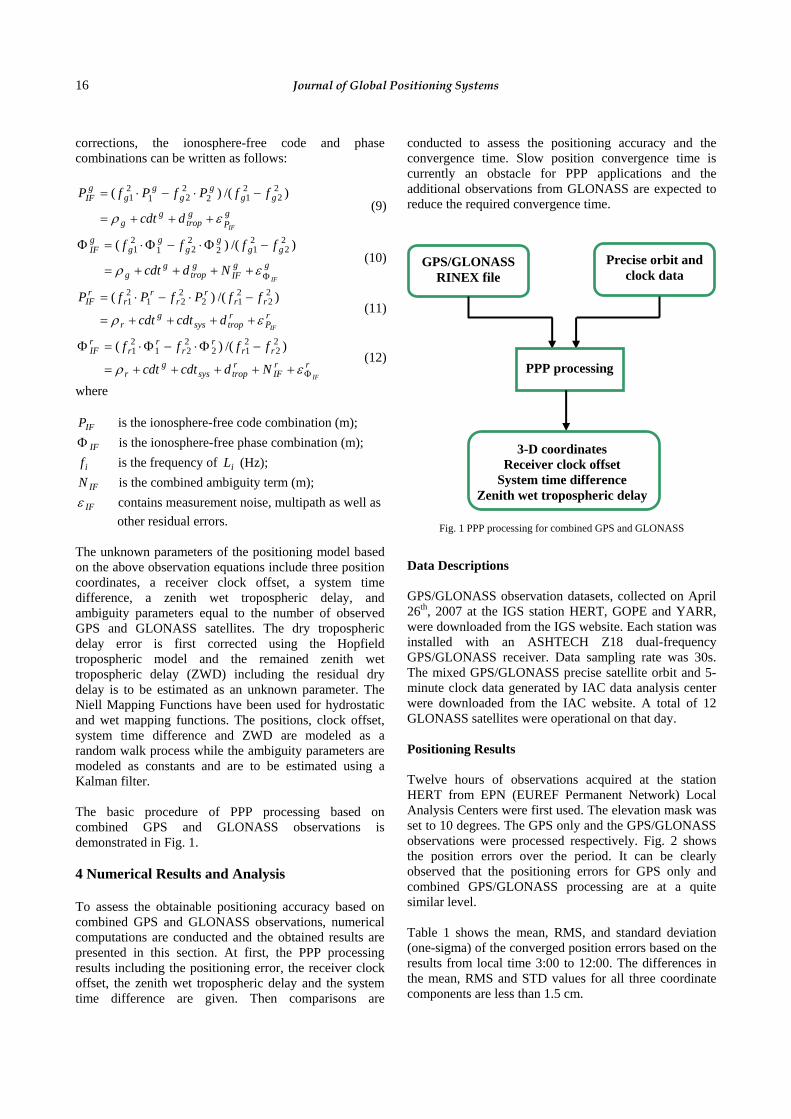
The unknown parameters of the positioning model based on the above observation equations include three position coordinates, a receiver clock offset, a system time difference, a zenith wet tropospheric delay, and ambiguity parameters equal to the number of observed GPS and GLONASS satellites. The dry tropospheric delay error is first corrected using the Hopfield tropospheric model and the remained zenith wet tropospheric delay (ZWD) including the residual dry delay is to be estimated as an unknown parameter. The Niell Mapping Functions have been used for hydrostatic and wet mapping functions. The positions, clock offset, system time difference and ZWD are modeled as a random walk process while the ambiguity parameters are modeled as constants and are to be estimated using a Kalman filter. The basic procedure of PPP processing based on combined GPS and GLONASS observations is demonstrated in Fig. 1.

4 Numerical Results and Analysis To assess the obtainable positioning accuracy based on combined GPS and GLONASS observations, numerical computations are conducted and the obtained results are presented in this section. At first, the PPP processing results including the positioning error, the receiver clock offset, the zenith wet tropospheric delay and the system time difference are given. Then comparisons are

conducted to assess the positioning accuracy and the convergence time. Slow position convergence time is currently an obstacle for PPP applications and the additional observations from GLONASS are expected to reduce the required convergence time.

Fig. 1 PPP processing for combined GPS and GLONASS

Data Descriptions GPS/GLONASS observation datasets, collected on April 26th, 2007 at the IGS station HERT, GOPE and YARR, were downloaded from the IGS website. Each station was installed with an ASHTECH Z18 dual-frequency GPS/GLONASS receiver. Data sampling rate was 30s. The mixed GPS/GLONASS precise satellite orbit and 5-minute clock data generated by IAC data analysis center were downloaded from the IAC website. A total of 12 GLONASS satellites were operational on that day. Positioning Results Twelve hours of observations acquired at the station HERT from EPN (EUREF Permanent Network) Local Analysis Centers were first used. The elevation mask was set to 10 degrees. The GPS only and the GPS/GLONASS observations were processed respectively. Fig. 2 shows the position errors over the period. It can be clearly observed that the positioning errors for GPS only and combined GPS/GLONASS processing are at a quite similar level. Table 1 shows the mean, RMS, and standard deviation (one-sigma) of the converged position errors based on the results from local time 3:00 to 12:00. The differences in the mean, RMS and STD values for all three coordinate components are less than 1.5 cm.

GPS/GLONASS RINEX file

Precise orbit and clock data

PPP processing

3-D coordinates Receiver clock offset

System time difference Zenith wet tropospheric delay


-1

0

1

Eas

t Erro

r (m

)

GPS OnlyGPS/GLONASS

-1

0

1

Nor

th E

rror (

m)

0:00 2:00 4:00 6:00 8:00 10:00 12:00-1

0

1

Up

Erro

r (m

)

GPS Time (HH:MM) Fig. 2 GPS only vs. GPS/GLONASS positioning errors

Tab. 1 Statistics of Position Results (m)

GPS Only GPS / GLONASS East 0.045 0.057

North 0.012 0.016 MEAN Up 0.012 0.001 East 0.016 0.014

North 0.006 0.006 STD Up 0.020 0.020 East 0.048 0.058

North 0.014 0.017 RMS Up 0.024 0.020

In addition to position determination, PPP can also output receiver clock offset solution which has the potential to support precise time transfer applications. The estimated receiver clock offsets in both GPS only and GPS/GLONASS processing are presented in Fig. 3. The red curve stands for the results from GPS only processing, which is completely overlapped by the green curve from the GPS/GLONASS processing results. Since the clock offset difference, which has a RMS value of 0.01 ns, is very small, the addition of GLONASS observations did not have a significant impact on the estimation of the receiver clock. Presented in Fig. 4 is the estimated zenith wet tropospheric delay. As can be seen, the ZWD difference between the GPS only processing and the combined GPS/GLONASS processing after the position convergence is not significant with a RMS value of 2 mm. The estimated system time difference is presented in Fig. 5. The system time difference varies in a range of about 4 ns over the twelve hours, which partially reflects the

accuracy of the GLONASS system time scale. The greater variation before the GPS time 2:00 is due to the position convergence process. The obtained system time difference from the combined GPS/GLONASS data processing in PPP includes not only the time difference between the GPS and GLONASS system times but also the receiver hardware delay differences between GPS and GLONASS. Since they can not be separated from each other, the obtained value is the combined system time difference and receiver’s inter-system hardware delay. As a result, the estimated system time difference should be considered as only an approximation to the true system time difference and is quite dependent on the receiver used.

0:00 2:00 4:00 6:00 8:00 10:00 12:000

20

40

60

80

100

120

Rec

eive

r clo

ck o

ffset

(ns)

GPS Time (HH:MM)

GPS OnlyGPS/GLONASS

Fig. 3 GPS only vs. GPS/GLONASS receiver clock offset estimates

0:00 2:00 4:00 6:00 8:00 10:00 12:000

0.1

0.2

0.3

Zeni

th w

et tr

opos

pher

ic d

elay

(m)

GPS Time (HH:MM)

GPS OnlyGPS/GLONASS

Fig. 4 GPS only vs. GPS/GLONASS zenith wet tropospheric delay estimates


0:00 2:00 4:00 6:00 8:00 10:00 12:00740

741

742

743

744

745

746

747

748

Sys

tem

tim

e di

ffere

nce

(ns)

GPS Time (HH:MM) Fig. 5 Estimated system time differences

Positioning Accuracy and Convergence Analysis

Four processing sessions, each with three-hour data from three IGS stations, namely HERT, GOPE and YARR, were included in the data analysis. The elevation masks were set to 10 degrees. For each session, in addition to the position errors, the PDOP value and the number of used satellites were also calculated. The computation of the PDOP values in GPS/GLONASS processing is based on the design matrix corresponding to the unknowns of the three position coordinates, the receiver clock offset and the system time difference. This design matrix has one more column compared to the design matrix used for PDOP computation in the GPS only processing. The processing results are presented in Figs. 6-17.

Fig. 6 shows the positioning results between 0:00 and 3:00 at HERT station. No significant PDOP improvement is found before the position solutions converge and as a result, no significant convergence improvement is found. Presented in Fig. 7 are the processing results from the GPS time 3:00 to 6:00. In this session, two GLONASS satellites were utilized on average. Although in the beginning the PDOP value has only a slight improvement by adding GLONASS observations, the convergence time has been reduced significantly in the east and up directions.

In Fig.e 8, although PDOP has a significant improvement from the local time 6:42 to 7:02, no significant convergence improvement is found. This is because such a geometry improvement with more visible satellites was present after the position solutions have already converged. Looking at the results in Fig. 9, the PDOP improvement occurred at the first half an hour and during the convergence process. As a result, it has reduced

significantly the position convergence time for horizontal coordinate components.

-101

Eas

t (m

)

-101

Nor

th (m

)

-101

Up

(m)

369

12

SV

s0:00 0:30 1:00 1:30 2:00 2:30 3:0005

1015

PD

OP

GPS Time (HH:MM)

GPS onlyGPS/GLO

Fig. 6 Processing results at HERT (Session 1)

-101

Eas

t (m

)

-101

Nor

th (m

)

-101

Up

(m)

369

12

SV

s

3:00 3:30 4:00 4:30 5:00 5:30 6:000246

PD

OP

GPS Time (HH:MM)

GPS onlyGPS/GLO


-101

Eas

t (m

)

-101

Nor

th (m

)

-101

Up

(m)

369

12

SV

s

6:00 6:30 7:00 7:30 8:00 8:30 9:000369

PD

OP

GPS Time (HH:MM)

GPS onlyGPS/GLO



-101

Eas

t (m

)

-101

Nor

th (m

)

-101

Up

(m)

369

12

SV

s

9:00 9:30 10:00 10:30 11:00 11:30 12:000246

PD

OP

GPS Time (HH:MM)

GPS onlyGPS/GLO


Table 2 shows the RMS statistics of the positioning errors at HERT station using the position results obtained from the last one and a half hours of observations from each session. A significant accuracy improvement is found in Session 2 where the improvements in the east and up components reach 4cm and 3cm respectively.

Tab. 2 RMS Statistics of Positioning Results at HERT (m)

GPS Only GPS / GLONASS East 0.101 0.093

North 0.031 0.034 Session 1 Up 0.082 0.092 East 0.129 0.087



North 0.012 0.011 Session 4 Up 0.013 0.013

Figs. 10-13 show the processing results at GOPE station. No convergence improvement is found in Fig. 10 while a slight improvement in the east component can be seen from Fig. 11. Look at Fig. 12, the convergence in the combined PPP processing appears more stable and smooth between 7:00 and 7:40 when compared to the GPS-only processing results. Fig. 13 indicates a slight improvement in the beginning of the convergence process.

-101

Eas

t (m

)

-101

Nor

th (m

)

-101

Up

(m)

369

12

SV

s

0:00 0:30 1:00 1:30 2:00 2:30 3:000246

PD

OP

GPS Time (HH:MM)

GPS onlyGPS/GLO

Fig. 10 Processing results at GOPE (Session 1)

-101

Eas

t (m

)

-101

Nor

th (m

)

-101

Up

(m)

369

12

SV

s

3:00 3:30 4:00 4:30 5:00 5:30 6:000246

PD

OP

GPS Time (HH:MM)

GPS onlyGPS/GLO


-101

Eas

t (m

)

-101

Nor

th (m

)

-101

Up

(m)

369

12

SV

s

6:00 6:30 7:00 7:30 8:00 8:30 9:000246

PD

OP

GPS Time (HH:MM)

GPS onlyGPS/GLO



-101

Eas

t (m

)

-101

Nor

th (m

)

-101

Up

(m)

369

12

SV

s

9:00 9:30 10:00 10:30 11:00 11:30 12:000246

PD

OP

GPS Time (HH:MM)

GPS onlyGPS/GLO


Presented in Table 3 is the RMS statistics of positioning results at GOPE station. The maximum accuracy improvement is 3cm which can be seen in the east component of Session 3 while the accuracy degradation of 2cm is also found in the up component of Session 1.

Tab. 3 RMS Statistics of Positioning Results at GOPE (m)

GPS Only

GPS / GLONASS

East 0.008 0.008 North 0.010 0.018 Session 1

Up 0.030 0.051 East 0.147 0.128



North 0.010 0.008 Session 4 Up 0.099 0.098

The processing results at YARR station are presented in Figs. 14-17. A significant convergence improvement has been found in the east direction in Fig. 14 where observations from an average of four GLONASS satellites are utilized in the combined processing during the period of 0:00 to 1:30. No convergence improvement is found in the other figures by adding the GLONASS observations due to limited number of visible GLONASS satellites. This indicates a correlation between position convergence improvement and satellite geometry improvement. Table 4 shows the RMS statistics results of the poisoning errors at YARR station. The maximum

accuracy improvement of 13cm occurs in the east direction of Session 1.

-101

Eas

t (m

)

-101

Nor

th (m

)

-101

Up

(m)

369

12

SV

s0:00 0:30 1:00 1:30 2:00 2:30 3:000246

PD

OP

GPS Time (HH:MM)

GPS onlyGPS/GLO

Fig. 14 Processing results at YARR (Session 1)

-101

Eas

t (m

)

-101

Nor

th (m

)

-101

Up

(m)

369

12

SV

s

3:00 3:30 4:00 4:30 5:00 5:30 6:000369

PD

OP

GPS Time (HH:MM)

GPS onlyGPS/GLO


-101

Eas

t (m

)

-101

Nor

th (m

)

-101

Up

(m)

369

12

SV

s

6:00 6:30 7:00 7:30 8:00 8:30 9:000246

PD

OP

GPS Time (HH:MM)

GPS onlyGPS/GLO



-101

Eas

t (m

)

-101

Nor

th (m

)

-101

Up

(m)

369

12

SV

s

9:00 9:30 10:00 10:30 11:00 11:30 12:000246

PD

OP

GPS Time (HH:MM)

GPS onlyGPS/GLO


Tab. 4 RMS Statistics of Positioning Results at YARR (m)

GPS Only

GPS / GLONASS

East 0.209 0.074 North 0.011 0.009 Session 1

Up 0.112 0.086 East 0.063 0.064



North 0.005 0.005 Session 4 Up 0.047 0.050

In order to compare the positioning accuracy between using GPS-only observations and combined GPS/GLONASS observations, the positioning accuracy derived from three-dimensional coordinate component errors is presented in Fig. 18. As can be seen, the improvement of the positioning accuracy is obvious for most of the position results, and the maximum improvement reaches 12cm.

0

0.1

0.2

0.3

Error (m)

GPS only

GPS/GLONASS

HERT GOPE YARR Fig. 18 Positioning accuracy comparison

5 CONCLUSIONS

A positioning model based on combined GPS and GLONASS observations has been proposed in this paper for precise point positioning. In order to assess the positioning accuracy and convergence time improvement of the combined GPS and GLONASS data processing, a 12-hour and four 3-hour sessions of datasets have been used in the data analysis. Comparisons have been conducted between GPS only and combined GPS/GLONASS processing. Based on the results, current GLONASS constellation has not caused a significant impact on the positioning results including position coordinates, receiver clock offset and zenith wet tropospheric delay since only two or three GLONASS satellites were observed most of time at any specific time. More significant improvements are expected when with more GLONASS satellites available in space. The research results further indicate that even with limited number of GLONASS satellites the improvement of the position convergence time is dependent on the improvement level of the satellite geometry for position determination. The results also indicate that the positioning accuracy can be improved by additional GLONASS observations in most cases. Further investigation will be conducted to assess the combined GPS/GLONASS precise point positioning in a kinematic mode.

ACKNOWLEDGMENTS

The financial supports from NSERC and GEOIDE are greatly appreciated. The contribution of data from the International GNSS Service (IGS) and Information- Analytical Center (IAC) is also appreciated.

Based on a paper presented at The Institute of Navigation International Technical Meeting, Fort Worth, Texas, September 2007.

REFERENCES

Bruyninx, C. (2007). Comparing GPS-only with GPS+GLONASS positioning in a Regional Permanent GNSS Network. GPS Solution, 11:97-106, 2007.

Habrich, H. (1999). Geodetic Applications of the Global Navigation Satellite System (GLONASS) and of GLONASS/GPS Combinations. PhD Thesis, University of Berne.

Habrich, H., P. Neumaier, K. Fisch (2004). GLONASS Data Analysis for IGS. Proceedings of IGS Workshop and Symposium, University of Berne, 2004.

Kaplan, E.D., C.J. Hegarty (2006). Understanding GPS: Principles and Applications. 2nd Edition. Artech House.


Oleynik, E.G., V.V. Mitrikas, S.G. Revnivykh, A.I. Serdukov, E.N.Dutov, V.F.Shiriaev (2006). High-Accurate GLONASS Orbit and Clock Determination for the Assessment of System Performance. Proceedings of ION GNSS 2006, Fort Worth, TX, September 26-29, 2006.

Romero, I., J.M.Dow, R. Zandbergen, J.Feltens, C.Garcia, H.Boomkamp, J.Perez (2004), The ESA/ESOC IGS Analysis Center Report 2002, IGS 2001-2002 Technical Report, 53-58, IGS Central Bureau, JPL-Publication, 2004.

Schaer, S.T., U. Hugentobler, R. Dach, M. Meindl, H. Bock, C.Urschl, G. Beutler (2004). GNSS Analysis at CODE. Proceedings of IGS Workshop and Symposium. University of Berne.

Sergey, K., R. Sergey, T. Suriya (2007). GLONASS as a Key Element of the Russian Positioning Service. Advances in Space Research, 39:1539-1544.

Tsujii, T., M. Harigae, T. Inagaki, T. Kanai (2000). Flight Tests of GPS/GLONASS Precise Positioning versus Dual Frequency KGPS Profile. Earth Planets Space, 52: 825-829.

Weber, R., E. Fragner (2002). The Quality of Precise GLONASS Ephemerides. Adv. Space Res. 30(2), 271-279, 2002.

Weber, R., J.A. Slater, E. Fragner, V. Glotov, H. Habrich, I.Romero, S. Schaer (2005). Precise GLONASS Orbit Determination within the IGS/IGLOS Pilot Project. Advances in Space Research, 36: 369-375.

Zinoviev, A.E (2005).Using GLONASS in Combined GNSS Receivers: Current Status. Proceedings of ION GNSS 2005, Long Beach, CA, September 13-16, 2005.

Journal of Global Positioning Systems (2007)Vol. 6, No. 1: 23-37Dierential GPS: the redu ed-dieren e approa hAndré LannesCentre National de la Re her he S ientiqueL2S, Supéle , 3, rue Joliot-Curie,91192 Gif-sur-Yvette edex (Fran e)Abstra t. In the traditional approa h to dierentialGNSS, the satellite error terms are eliminated by form-ing the so- alled single dieren es (SD). One then getsrid of the re eiver error terms by omputing, for ea hre eiver to be onsidered, the orresponding double dif-feren es (DD): the dis repan ies between the single dier-en es (SD) and one of them taken as referen e. To han-dle the SD's in a homogeneous manner, one may equallywell onsider the dis repan ies between the SD's and theirmean value. In this paper, these ` entralized dierentialdata' are referred to as `redu ed dieren es' (RD). In the ase where the GNSS devi e in ludes only two re eivers,this approa h is ompletely equivalent to `double entral-ization.' More pre isely, the information ontained in the`double entralized observations' is then a simple anti-symmetri trans ription of that ontained in the redu eddieren es. The ambiguities are then rational numberswhi h are related to the traditional integer ambiguitiesin a very simple manner. The properties established inthis paper shed a new light on the orresponding analysis.(The extension to GNSS networks with missing data willbe presented in a forth oming paper.) The orrespondingappli ations on ern the identi ation of outliers in realtime. Cy le slips ombined with mis ellaneous SD biases an thus be easily identied.Key words. GNSS, DGPS, entralized undierentialmethods, RTK. Data assimilation, DIA.1 Introdu tionThe global positioning te hniques are based on the fol-lowing observational equations. For ea h frequen y fν ,for ea h re eiver-satellite pair (r, s), and at ea h epo h t,the ode and arrier-phase data are respe tively of theform (e.g., Se t. 14 in Strang and Borre 1997)pν,t(r, s) = ρt(r, s) + c[dtν,t(r) − dtν,t(s)] + ǫν,t(r, s) (1)

φν,t(r, s) = ρt(r, s) + c[δtν,t(r) − δtν,t(s)]

+ λν [ϕν,0(r) − ϕν,0(s)] + λνNν(r, s) + εν,t(r, s)(2)In these equations, whi h are expressed in length units,

ρt(r, s) is the re eiver-satellite range: the distan e be-tween satellite s (at the time t−τ where the signal is emit-ted) and re eiver r (at the time t of its re eption). Clearly,the λν 's denote the wavelengths of the arrier waves; therational integersNν(r, s) are the integer arrier-phase am-biguities. The instrumental delays and lo k errors thatfor a given (ν, t) depend only on r and s are lumped to-gether in the re eiver and satellite error terms dtν,t(r),dtν,t(s) for the ode, and δtν,t(r), δtν,t(s) for the phase(c is the speed of light); ϕν,0(r) and ϕν,0(s) are the initialphases (expressed in y les) in re eiver r and satellite s,respe tively. Here, for larity, the ionospheri and tropo-spheri delays are ignored. At this introdu tory level, wethus onsider that the data have been orre ted for thesedelays. Clearly, the ode and phase errors ǫν,t(i, j) andεν,t(i, j) in lude both noise and residual model errors.For our present purposes, we now on entrate on Equa-tion (2) in the single-frequen y mode:φt(r, s) = ρt(r, s) + c[δtt(r) − δtt(s)]

+ λ[ϕ0(r) − ϕ0(s)] + λN(r, s) + εt(r, s)(3)In what follows, a notation su h as a := b means à isequal to b by denition.' Let r1 now be the referen e re- eiver, and r2 be that of the user. Denote by s1, s2, . . . , snthe satellites involved in the GPS devi e. A quantitysu h as

ϑj := ϑ(r2 , sj)− ϑ(r1 , sj) (4)is then referred to as a single dieren e (SD) in ϑ. By us-ing this notation, Equation (3) then yieldsφjt = ρjt + c[δtt(r2)− δtt(r1)]

+ λ[ϕ0(r2)− ϕ0(r1)] + λaj + εjt(5)where

aj := N j (6)One thus gets rid of the satellite error terms. The aj 'sare the integer ambiguities of the SD phase data.

24 Journal of Global Positioning Systems1.1 Basi notions1.1.1 Double dieren esIn the traditional approa h to dierential GNSS, one rstsele ts a referen e satellite. Here, this satellite is denotedby sk . A quantity su h asϑjk := ϑj − ϑk (i 6= j) (7)is then referred to as a double dieren e (DD) in ϑ (seeFig. 1).By subtra ting from Eq. (5) its expression for j = k(term by term), one then obtains the relationφjt;k = ρjt;k + λajk + εjt;k (ajk ∈ Z) (8)One thus gets rid of the re eiver error terms. The ajk 'sare said to be the DD integer ambiguities of the problem.

ϑjk

ϑk ϑj

-r

0Fig. 1 Notion of double dieren e. Thedouble dieren e ϑj

k is the value of the sin-gle dieren e ϑj by taking as origin (orreferen e) the value of the single dier-en e ϑk.1.1.2 Redu ed dieren esIn the approa h presented in this paper, we onsider ahomogeneous way of eliminating the re eiver error terms.The idea is to onsider the quantities (see Fig. 2)ϑj0 := ϑj − ϑ0 (9)where ϑ0 is the mean value of the ϑj :ϑ0 :=

1

n

n∑

j=1

ϑj (10)r

ϑ0

ϑj0

ϑj

-r

0Fig. 2 Notion of redu ed dieren e. Theredu ed dieren e ϑj0 is the value of thesingle dieren e ϑj by taking as origin (orreferen e) the mean value ϑ0 of the singledieren es ( ompare with Fig. 1).Clearly, this bary entri value an be regarded as a vir-tual SD asso iated with a virtual referen e satellite s0 .A ording to a well-known bary entri property (for fur-ther details see Se t. 3), for any k, we have

n∑

j=1

|ϑj0|2 ≤

∑

j 6=k

|ϑjk|2 (11)

The ϑj0 's an therefore be referred to as `redu ed dier-en es' (RD).Subtra ting from Eq. (5) its expression in terms of meanvalues (term by term), we then obtain the relation similarto Eq. (8)φjt;0 = ρjt;0 + λaj0 + εjt;0 (aj0 ∈ Q) (12)Note that the RD ambiguities aj0 's are rational numbers(and not in general rational integers).1.1.3 Dierential observationsBy onstru tion, the DD's of the fun tionϑd(ri , sj) :=

0 if i = 1 or j = k;

ϑjk otherwise. (13)are the DD's of the fun tion ϑ(ri , sj). Su h a fun tion antherefore be referred to as a `dierential observational'(DO) fun tion.1.1.4 Redu ed observationsBy onstru tion, the SD's of the fun tionϑr(ri , sj) :=

0 if i = 1;

ϑj0 otherwise. (14)are the redu ed dieren es of the fun tion ϑ(ri , sj). Su ha fun tion an therefore be referred to as a `redu ed ob-servational' (RO) fun tion.1.1.5 Centralized observationsIn the ` entralized observational approa h' of Shi andHan (1992), one gets rid of the satellite error terms byforming the single entralized observationsϑ(1)

c (ri , sj) = ϑ(ri , sj)−1

2

2∑

i=1

ϑ(ri , sj)

= (−1)i1

2[ϑ(r2 , sj)− ϑ(r1 , sj)]

= (−1)iϑj

2The re eiver error terms are then eliminated by formingthe double entralized observationsϑ(2)

c (ri , sj) = ϑ(1)c (ri , sj)−

1

n

n∑

j=1

ϑ(1)c (ri , sj)

= (−1)i1

2

(ϑj −

1

n

n∑

j=1

ϑj)

= (−1)iϑj02

Lannes: Dierential GPS The redu ed dieren e approa h 25One is then led to say thatϑc(ri , sj) := (−1)i

ϑj02

(15)is a entralized observational fun tion. In the ase wherethe GNSS devi e in ludes only two re eivers, the informa-tion ontained in the entralized observations is thereforea simple àntisymmetri trans ription' of that ontainedin the redu ed dieren es. The title of the paper was hosen a ordingly.1.2 ContentsThe theoreti al framework of this ontribution is pre-sented in Se t. 2. As laried in Se t. 3, the DD andRD approa hes prove to be equivalent. In parti ular, al-though the RD ambiguities are rational numbers, the am-biguity problems to be solved are the same. Se tion 5.2is devoted to this point. The RD approa h should how-ever be preferred. Indeed, as shown in Se t. 4, it re-veals interesting properties whi h give a deeper insightinto the problem. These properties, whi h are maskedin the DD approa h, shed a new light on the entral-ized undierential method of Shi and Han (1992). Theyalso omplete the dual algebrai approa h of Lannes andDurand (2003). As a result, these equivalent approa hes an benet from ea h other. As shown in Se t. 6, one ofthese properties plays a key role in the DIA pro eduresof the data assimilation pro esses presented in Se t. 5.The SD biases, among whi h the y le slips (if any), anthen be identied in real time. Related omments are tobe found in Se t. 7. As pointed out in that se tion, theanalysis presented in this paper an be regarded as anintrodu tion to the ase of GNSS networks with missingdata (Lannes 2008).2 Theoreti al frameworkIn the ontext dened in Se t. 1, the notion of observa-tional spa e an be spe ied as follows.2.1 Observational spa esIn what follows, it may be onvenient to onsider that afun tion su h as ϑ(r, s) takes its values on a re tangulargrid. When the GNSS devi e in ludes two re eivers andn satellites, this grid in ludes two lines and n olumns;ϑ is then regarded as a ve tor of the observational spa eE := R2n. Clearly, these values are the omponents of ϑin the standard basis of E. The notation Eψ spe iesthe nature of the ve tors ϑ of E: ψ = p for the ode,ψ = φ for the phase. The varian e- ovarian e matrix ofthe orresponding data ve tor is denoted by Vψ; Vψ is theoperator on E indu ed by Vψ . One is then led to denethe òbservational data spa e' of type ψ as the spa e E+

ψwith inner produ t〈ϑ | ϑ′〉E+

ψ:= (ϑ · V −1

ψ ϑ′)E (16)Clearly, E+ ≡ E+

ψ is a real Hilbert spa e.

2.1.1 Nuisan e delay spa eIn what follows, the spa e E0 of fun tions ϑ(ri , sj) of theform ϕ(sj) − ϕ(ri) is referred to as the nuisan e delayspa e (see Eqs. (1), (2) and Fig. 4). In the spe ial aseunder onsideration (with two re eivers), this subspa eof E is of dimension n+ 1.2.1.2 Clean observational spa esThe orthogonal omplement of E0 in E, denoted by Ec ,is referred to as the ` lean observational (CO) spa e.'The orthogonal omplement of E0 in E+ , E+

c , is thenreferred to as the `CO data spa e' (see Fig. 4). In thespe ial ase under onsideration, Ec and E+

c are of di-mension 2n − (n + 1) = n − 1. As shown below, Ec isthen the spa e of ` entralized observational fun tions' ϑcdened by Eq. (15).Proof. In the Eu lidean spa e E, ϑc is orthogonal to anynuisan e fun tion of E0 . Indeed,2∑

i=1

n∑

j=1

[ϕ(sj)− ϕ(ri)](−1)iϑj0 =

n∑

j=1

ϑj0ϕ(sj)

2∑

i=1

(−1)i

−2∑

i=1

(−1)iϕ(ri)

n∑

j=1

ϑj0with ∑2i=1(−1)i = 0 and ∑n

j=1 ϑj0 = 0. The propertythen follows from the fa t that the fun tions ϑc form aspa e of dimension n− 1.Remark 2.1.2. Let Pc be the orthogonal proje tionof E onto Ec . Here, the entralized observational fun -tion ϑc dened by Eq. (15) is the proje tion of ϑ on Ec:

ϑc := Pcϑ. In other terms, the ` leaning operator' Pc thenredu es to the `double- entralization operator.' This doesnot hold for GNSS networks with missing data. The ter-minology was hosen a ordingly. Depending on the on-text, C and subs ript stand for ` lean' or ` entralized.'2.2 SD spa eDenoting by b := ejnj=1 the standard basis of Rn, letus onsider the ve tor ϑ :=

∑nj=1 ϑ

jej in whi h the ϑj 'sare the single dieren es dened in Eq. (4). Clearly, su ha ve tor an be regarded as a SD ve tor. In this ontext,we say that F := Rn is the `SD spa e' (see Fig. 3).2.2.1 SD operatorThe SD operator is the operator from E+ into F denedby the relation (see Eq. (4))Sϑ := ϑ i.e. (Sϑ)j := ϑj (17)We now denote by S† the orresponding `ba kproje tion'operator, i.e., the operator from F into E(S†ϑ)(ri , sj) := (−1)iϑj (18)

26 Journal of Global Positioning SystemsFor any ϑ ∈ F , the fun tion ϑ′ := S†ϑ/2 is su h thatSϑ′ = ϑ; S is therefore surje tive.In what follows, Vψ is the varian e- ovarian e matrix ofthe SD data ve tor ψ := Sψ. Denoting by Vψ the oper-ator on F indu ed by Vψ , we haveVψ = SVψS

† (19)We now show that the adjoint of S is given by the relationS∗ = VψS

† (20)hen e, from Eq. (19),SS∗ = Vψ (21)Proof. By denition, S∗ is the operator from F into E+su h that for any ϑ′ ∈ E+ and any ϑ ∈ F , we have

(Sϑ′ · ϑ)F = 〈ϑ′ | S∗ϑ〉E+ . Clearly,(Sϑ′ · ϑ)F =

n∑

j=1

[ 2∑

i=1

(−1)iϑ′(ri , sj)]ϑjFrom Eq. (18), we therefore have

(Sϑ′ · ϑ)F =

2∑

i=1

n∑

j=1

ϑ′(ri , sj)(S†ϑ)(ri , sj)i.e., (Sϑ′ · ϑ)F = (ϑ′ · S†ϑ)E =(ϑ′ · [V −1

ψ Vψ ]S†ϑ)E. Asa result,

(Sϑ′ · ϑ)F = 〈ϑ′ | VψS†ϑ〉E+hen e S∗ = VψS

† .2.2.2 RD spa e and RD ambiguity latti eLet us denote by F0 the spa e of ve tors ϑ ∈ F whose omponents ϑj are identi al. The orthogonal omplementof F0 into F is the spa e (see Fig. 3)Fr :=

ϑ ∈ F :

∑nj=1 ϑ

j = 0As F0 is a one-dimensional spa e, Fr is of dimension n−1.Let Q0 and Qr be the orthogonal proje tions of F onto F0and Fr , respe tively. Clearly, these operators are expli -itly dened by the relations

(Q0ϑ)j = ϑ0 (Qrϑ)j = ϑj − ϑ0 (22)where ϑ0 is the mean value of the ϑj 's. With regard tothe RD approa h, we are then led to set (see Eqs. (9),(10), (22) and Fig. 3)ϑr := Qrϑ (23)Clearly, the omponents of ϑr in basis b are the n re-du ed dieren es ϑj0 ; Fr an therefore be referred to asthe `RD spa e.' Note that ϑc is related to ϑr by therelation ϑc = S†ϑr/2 (see Eqs. (15) and (18)).

As ϑr is the proje tion of ϑ on Er , we haven∑

j=1

|ϑj0|2 =

n∑

j=1

|ϑj − ϑ0|2 = infϑo∈R

n∑

j=1

|ϑj − ϑo|2The property expressed in Eq. (11) results from this re-lation.The proje tion of Zn onto Fr is a latti e of rank n− 1: the`RD ambiguity latti e' Lr (see Fig. 3). In basis b (whi his not a basis of Lr), the omponents of a point ar of Lrare rational numbers: the n rational ambiguities aj0 .Remark 2.2.2. The RO fun tions ϑr dened by Eq. (14)form a subspa e of E denoted by Er (see Fig. 4). Clearly,this `RO spa e' is a simple insertion of Fr in E.2.2.3 DD spa e and DD ambiguity latti eIn the DD approa h, k being xed, one is led to onsiderthe subspa e of F (see Fig. 3)Fd := ϑ ∈ F : ϑk = 0By onstru tion, Fd is isomorphi to Rn−1. Let Qd nowbe the oblique proje tion of F onto Fd along F0 . Notethat Qd is expli itly dened by the relation(Qdϑ)j = ϑj − ϑk (24)We are then led to set (see Eq. (7) and Fig. 3)ϑd := Qdϑ (25)Let bd := ejj 6=k be the standard basis of Fd . As the omponents of ϑd in basis bd are the n− 1 double dier-en es ϑjk , Fd an be regarded as a `DD spa e.'The interse tion of Zn with Fd is a latti e of rank n− 1:the `DD ambiguity latti e' Ld (see Fig. 3). In basis bd ,the omponents of a point ad of Ld are rational integers:the n− 1 integer ambiguities ajk (j 6= k).Clearly, Ld = QdLd hen e Ld ⊂ QdZn (sin e Ld is asubset of Zn). Furthermore, QdZn ⊂ Ld . We thereforehave Ld = QdZn. As Lr := QrZ

n and Qr = QrQd ,it follows that Lr = QrLd (see Fig. 3).Remark 2.2.3. The DO fun tions ϑd dened by Eq. (13)form a subspa e of E denoted by Ed (see Fig. 4). Clearly,this `DO spa e' is an insertion of Fd in E.2.3 RD and DD operatorsThe RD operator is the operator from E+ into Fr denedby the relationSr := QrS (26)Note that Sr is surje tive. (The argument is the sameas that used for S .) As expe ted, the null spa e of Sr(denoted by kerSr) is the nuisan e delay spa e E0 . Thisproperty an be expli itly established as follows.

Lannes: Dierential GPS The redu ed dieren e approa h 27Proof. Clearly, E0 ⊂ kerSr with dimE0 = n+ 1; butdim(kerSr) = dimE − dimFr = 2n− (n− 1) = n+ 1hen e the property.The DD operator is the operator from E+ into Fd denedby the relationSd := QdS (27)Like Sr , Sd is surje tive, and kerSd = E0 .3 Equivalen e of the DD and RDapproa hesThe spa es Fd and Fr are isomorphi . More pre isely,the restri tion of Qr to Fd , the operator from Fd into Frdened by the relationRϑd := Qrϑd (28)maps Fd onto Fr , and Ld onto Lr (see Fig. 3). Its inverseis the operator from Fr into Fd

Dϑr := Qdϑr (29)Note that the a tion of DR orresponds to the su essive hanges of origin ϑk → ϑ0 → ϑk (see Figs. 1 and 2):(DRϑd)j = (ϑjk − ϑ

0)− (ϑkk − ϑ0) = ϑjkThe ve tors erj := Rej (j 6= k) form a basis of Fr , whi his also a basis of Lr : the basis brd := Rbd . In this ba-sis, the omponents of a ve tor ϑr of Fr are the ompo-nents ϑjk of ϑd = Dϑr . Indeed,

ϑr = Rϑd = R∑

j 6=k

ϑjkej =∑

j 6=k

ϑjkRej =∑

j 6=k

ϑjkerjIn parti ular, in this basis (whi h is not orthogonal), the omponents of a point ar of Lr are the n− 1 integer am-biguities ajk of ad = Dar . We re all that in the standardbasis of F (whi h is not a basis of Lr), the omponentsof ar are the n rational ambiguities aj0 .Let T now be the orthogonal proje tion of F onto Fdrestri ted to Fr (see Fig. 3). For any ϑ′ in Fr and any ϑin Fd , we have (ϑ′ · ϑ)F = (ϑ′ · Rϑ)F = (Tϑ′ · ϑ)F .This shows that, T is the adjoint of R on F : R† = T .Expli itly,(R†ϑr)

j = ϑj0 (∀j 6= k); (R†ϑr)k = 0 (30)As D is the inverse of R, D† is the inverse of R†:

(D†ϑd)j = ϑjk (∀j 6= k); (D†ϑd)k = −∑

j 6=k

ϑjk (31)Let Vψd now be the varian e- ovarian ematrix (expressedin basis bd) of the DD data ψd . Likewise, let Vψr be the

?R6D

@@I

0

ϑ ← SD: ϑ1, . . . , ϑn

ϑd ← DD: ϑ1

k , . . . , ϑnk

ϑr ← RD: ϑ10 , . . . , ϑn0

F := Rn

Fd

ekFr

F0

r r r

s

s

s

ad

ar

s→ Ld

r→ Lr

@@@@ITFig. 3 Geometri al representation of the main elements in-volved in the equivalen e of the DD and RD approa hes.Here, ek is the ve tor of the standard basis of R

n asso i-ated with the referen e satellite. Note that ϑkk = 0 andPn

j=1ϑj0 = 0 (see Figs. 1 and 2, respe tively); R is the or-thogonal proje tion of F onto Fr restri ted to Fd; R standsfor `redu tion.' Its inverse, D, is the oblique proje tionof F onto Fd (along F0) restri ted to Fr; D stands for`dieren e.' The adjoint of R is the orthogonal proje tionof F onto Fd restri ted to Fr: R†

= T . Its inverse is theadjoint of D: D†. Further details (in parti ular those on- erning latti es Ld and Lr) are to be found in Se ts. 2 and 3.varian e- ovarian e matrix (expressed in basis b) of theRD data ψr . In what follows, Vψd is the operator on Fdindu ed by Vψd . Likewise, Vψr is the operator on Fr in-du ed by Vψr . Let Qr now be the matrix of Qr expressedin basis b. As Vψr = QrVψQTr = QrVψQr , the opera-tor Vψr is the operator on Fr expli itly dened by therelation

Vψrϑ = QrVψϑ (ϑ ∈ Fr) (32)With regard to the least-squares (LS) problems to bedealt with, Fd and Fr are then equipped with the innerprodu ts (see the lower part of Fig. 4)〈ϑ′

d | ϑd〉Fψ;d+:= (ϑ′

d · ϑd+)F ϑd+ := V −1

ψd ϑd (33)〈ϑ′

r | ϑr〉Fψ;r+:= (ϑ′

r · ϑr+)F ϑr+ := V −1ψr ϑr (34)As E+ ≡ E+

ψ is referred to as the observational data spa eof type ψ, we may say that Fd+ ≡ Fψ;d+ is a `DD dataspa e' of type ψ. Likewise, Fr+ ≡ Fψ;r+ is the `RD dataspa e' of type ψ.We have Vψd = DVψrD†, hen e

V −1ψd = R†V −1

ψr RAs illustrated in the lower part of Fig. 4, it follows thatϑd+ = R†ϑr+ (35)ϑr+ = D†ϑd+ (36)

28 Journal of Global Positioning SystemsFrom Eqs. (33) and (35), 〈ϑ′d | ϑd〉Fd+

= (ϑ′d · R

†ϑr+)F ;hen e 〈ϑ′d | ϑd〉Fd+

= (Rϑ′d · ϑr+)F . We thus have

〈ϑ′d | ϑd〉Fd+

= 〈ϑ′r | ϑr〉Fr+where ϑ′

r = Rϑ′d and ϑr = Rϑd . In parti ular,

‖ϑd‖2Fd+

= ‖ϑr‖2Fr+

(for ϑr = Rϑd) (37)The DD and RD approa hes are therefore ` ompletelyequivalent.' This said, as shown in Se t. 4 (see, in parti -ular, Result 4.2.2), the RD approa h reveals interestingproperties whi h are ompletely hidden in DD mode (seeRemark 4.2.2).4 Observational equivalen e:Duality4.1 Proje tion onto the CO data spa eLet ϑ be some point in the observational spa e E. In whatfollows, ϑ+

c denotes the orthogonal proje tion of ϑ on theCO data spa e E+

c (see Se t. 2.1.2 and Fig. 4):ϑ+

c := P+

c ϑ (38)Clearly, P+

c is the orresponding orthogonal proje tion.Let ϑr := Srϑ now be the RD ve tor of ϑ. The solutionsof the equation Srϑ′ = ϑr are dened up to a ve tor of E0 ;

ϑ+

c is the solution with smallest norm in E+. The operatorthat maps ϑr to ϑ+

c is referred to as the Moore-Penrosepseudoinverse of Sr . This operator is denoted by S+r :

ϑ+

c = S+r ϑr (39)Likewise, for ϑd = Dϑr , we have ϑ+

c = S+d ϑd . Clearly,

ϑ+

c an be regarded as the expression for ϑr (or ϑd)brought ba k to E+ via S+r (or S+

d ). In this ontext,we dene ϑc+ as follows (see Eqs. (34), (18) and Fig. 4):ϑc+ := S†ϑr+ (40)The following property then ompletes the analysis pre-sented in Se t. 3.Property 4.1. One has ϑ+

c = Vψϑc+ . As a orollary,‖ϑ+

c ‖2E+ = (ϑ+

c · ϑc+)E = ‖ϑr‖2Fr+

.Proof. As Sr is surje tive, its pseudoinverse is given bythe relationS+

r = S∗r (SrS

∗r )−1For any ϑ in Fr , we have (sin e Sr = QrS)

S∗rϑ = (QrS)∗ϑ = S∗Q∗

rϑ = S∗Qrϑ = S∗ϑwhere S∗ = VψS† (Eq. (20)). As a result (see Eqs. (21)and (32)),

SrS∗rϑ = QrSS

∗ϑ = QrVψϑ = Vψrϑ

It then follows thatS+

r = S∗r V

−1ψrhen e

ϑ+

c = S∗r V

−1ψr ϑr = S∗V −1

ψr ϑr = VψS†V −1ψr ϑri.e., ϑ+

c = Vψϑc+ (from Eqs. (34) and (40)). As a orollary(see Eq. (16)),‖ϑ+

c ‖2E+ = 〈ϑ+

c | ϑ+

c 〉E+

= 〈ϑ+

c | Vψϑc+〉E+ = (ϑ+

c · ϑc+)EAs ϑc is the proje tion of ϑ+

c on Ec (see Fig. 4), we have(see Eqs. (40) and (18))(ϑ+

c · ϑc+)E = (ϑc · ϑc+)E

= (ϑc · S†ϑr+)E

= (Sϑc · ϑr+)FBut, from Eq. (15), Sϑc = ϑr . As a result,‖ϑ+

c ‖2E+ = (ϑr · ϑr+)F = ‖ϑr‖

2Fr+4.2 Analysis of a typi al situationTo illustrate our analysis, we now onsider the ase wherethe varian e- ovarian e matrix of the observational dataof type ψ is of the form

Vψ = diag(η(ri , sj)σ2ψ

) (41)Clearly, σ2ψ is a `referen e varian e;' η(r, s) is a nonnega-tive weight fun tion. The varian e- ovarian e matrix ofthe SD data ψ := Sψ is then given by the relation

Vψ = diag(ηjσ2ψ) ηj := η(r1 , sj) + η(r2 , sj) (42)As laried in Remark 4.2.1, the following results shedsa new light on the entralized observational approa h ofShi and Han (1992). The dual approa h of Lannes andDurand (2003) is also thereby enri hed.Result 4.2.1. Denoting by ϑjr+ and ϑjr the omponentsof ϑr+ and ϑr , respe tively, we have

ϑjr+ =1

ηjσ2ψ

(ϑjr − δϑ) (ϑjr ≡ ϑj0)where

δϑ :=

n∑

j=1

µjϑjr µj :=

1ηj∑nj=1

1ηjAs a orollary, ϑ+

c = ησ2ψ ϑc+ = ησ2

ψ S†ϑr+ .Proof. By denition, ϑr+ := V −1

ψr ϑr (Eq. (34)). Toidentify the inverse of Vψr on Fr , we solve the equationVψrϑ

′ = ϑr in Fr . From Eq. (32), Vψrϑ′ is equal to Vψϑ′up to a ve tor of F0 . It then follows from Eq. (42) thatthe omponents of ϑ′ are related to those of ϑr by therelation

ηjσ2ψϑ

′j = ϑjr − δ

Lannes: Dierential GPS The redu ed dieren e approa h 29where δ is some onstant in R. As result,ϑ′j =

1

ηjσ2ψ

(ϑjr − δ)As ϑ′ lies in Fr , we have∑nj=1 ϑ

′j = 0, hen e the identityδ ≡ δϑ . The result and its orollary then follow fromProperty 4.1 and Eqs. (40, (41).It is important to note that in the spe ial ase where theweights η(ri , sj) are all equal to unity, we have ηj = 2,µj = 1/n for all j, and δϑ = 0 .Result 4.2.2. The square of the norm ϑr in Fr+ an beexpanded as follows:‖ϑr‖

2Fr+

=

n∑

j=1

1

ηjσ2ψ

(ϑjr − δϑ)2Proof. From Property 4.1, Eq. (41) and Result 4.2.1,we have

‖ϑr‖2Fr+

= (ϑ+

c · ϑc+)E

=2∑

i=1

n∑

j=1

η(ri , sj)σ2ψ ϑ

2c+(ri , sj)

=

n∑

j=1

2∑

i=1

η(ri , sj)1

η2jσ

2ψ

(ϑjr − δϑ)2

=

n∑

j=1

[η(r1 , sj) + η(r2 , sj)]1

η2jσ

2ψ

(ϑjr − δϑ)2The result then follows from the fa t that

η(r1 , sj) + η(r2 , sj) = ηj ; see Eq. (42).Remark 4.2.1. Property 4.1 illustrated by Results 4.2.1and 4.2.2 gives a `dual insight' into the problem (seeFig. 4). For example, in the DIA method presented inSe t. 6, ϑr is the [ψν,t]- omponent of a residual quan-tity involved in a LS problem stated in (the Hilbert sumof) [ψν,t]- opies of Fr+ . A ording to Property 4.1, stat-ing the problem in that way amounts to stating it in(the Hilbert sum of) [ψν,t]- opies of E+

c . Depending onthe ontext, one may thus operate in various equivalentways. Indeed, equipped with appropriate inner produ ts,the spa es Fr+ , Fd+ , Er+ , Ed+ and Ec+ are isomorphi to E+

c .Let us now ome ba k to the spe ial ase where the weightsη(ri , sj) are all equal to unity. Result 4.2.1 then yields(see also Eqs. (15) and (18)):ϑ+

c = ϑc =1

2S†ϑr (43)Clearly, the CO data spa e E+

c then oin ides with theCO spa e Ec (see Fig. 4). A ording to Result 4.2.2, we

0

ϑr

ϑ+

c

ϑ

ϑd

ϑc

ϑc+

E

Ed

Er

E+

c

Ec

E0

?

Sr

?

Sd

0

ϑ

ϑd

ϑr

F

Fd

Fr

F0

ϑd+

@@ϑr+

Srϑc+Fig. 4 Dual representation of the main elements of the prob-lem. Here, E0 is the nuisan e delay spa e (see Se t. 2.1.1).This subspa e of the observational spa e E is the nullspa e of the RD (and DD) operators Sr (and Sd); seeSe t. 2.3; ϑc is the proje tion of ϑ on the orthogonal om-plement of E0 in E, the CO spa e Ec: ϑc = Pcϑ. In the ase where the GNSS devi e in ludes only two re eivers,

ϑc is the entralized observational fun tion ϑc dened viaEq. (15); see Remark 2.1.2. Here, ϑr is the observationalversion of #r (see Remark 2.2.2). Likewise, ϑd is the ob-servational version of #d (see Remark. 2.2.3). The pseu-doinverse of Sr maps Fr onto the CO data spa e E+c ,the orthogonal omplement of E in the observational dataspa e E+: ϑ+

c = S+r #r = P+

c ϑ. A ording to Property 4.1.1,one has ϑ+c = Vψϑc+ where ϑc+ := S†

#r+ with #r+ := V −1 r #r ;note that Srϑc+ = Sϑc+ = SS†

#r+ = 2#r+ . Likewise,S+

d maps Fd onto E+c : ϑ+

c = S+d #d . In the important spe- ial ase examined in Remark 4.2.1, ϑ+

c oin ides with ϑc(see Eq. (43)); E+c then oin ides with Ec .then have (see also Eq. (37)):

‖ϑ+

c ‖2E+ = ‖ϑr‖

2Fr+

= ‖ϑd‖2Fd+

=

n∑

j=1

1

2σ2ψ

|ϑjr |2 (44)The orthogonal proje tion of E+ onto E+

c is also basi allyinvolved in the dual algebrai formulation of Lannes andDurand (2003); see Fig. 4 of their paper. The key re-sult (43) ompletes their ontribution. To establish this

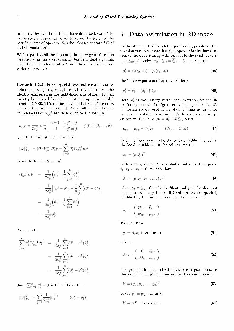
30 Journal of Global Positioning Systemsproperty, these authors should have des ribed, expli itly,in the spe ial ase under onsideration, the a tion of thepseudoinverse of operator Sd (the ` losure operator' C oftheir formulation).With regard to all these points, the more general resultsestablished in this se tion enri h both the dual algebrai formulation of dierential GPS and the entralized obser-vational approa h.Remark 4.2.2. In the spe ial ase under onsideration(where the weights η(ri , sj) are all equal to unity), theidentity expressed in the right-hand side of Eq. (44) andire tly be derived from the traditional approa h to dif-ferential GNSS. This an be shown as follows. For larity, onsider the ase where k = 1. As is well known, the ma-trix elements of V −1ψd are then given by the formula

κj,j′ =1

2σ2ψ

×1

n

∣∣∣∣∣n− 1 if j′ = j

−1 if j′ 6= jj, j′ ∈ 2, . . . , nClearly, for any ϑ in Fd , we have

‖ϑ‖2Fd+= (ϑ · V −1

ψd ϑ)F =

n∑

j=2

ϑjk(V−1ψd ϑ)jin whi h (for j = 2, . . . , n)

(V −1ψd ϑ)j =

1

2σ2ψ

(ϑjk −

1

n

n∑

j=2

ϑjk

)

=1

2σ2ψ

[(ϑj − ϑk)−

1

n

n∑

j=1

(ϑj − ϑk)]

=1

2σ2ψ

(ϑj −

1

n

n∑

j=1

ϑj)

=1

2σ2ψ

ϑj0As a result,n∑

j=2

ϑjk(V−1ψd ϑ)j =

1

2σ2ψ

n∑

j=2

(ϑj − ϑk)ϑj0

=1

2σ2ψ

n∑

j=1

(ϑj − ϑk)ϑj0

=1

2σ2ψ

n∑

j=1

(ϑj0 − ϑk0)ϑ

j0Sin e ∑n

j=1 ϑj0 = 0, it then follows that

‖ϑ‖2Fd+=

n∑

j=1

1

2σ2ψ

|ϑj0|2 (ϑj0 ≡ ϑ

jr)

5 Data assimilation in RD modeIn the statement of the global positioning problems, theposition variable at epo h t, ξt , appears via the lineariza-tion of the quantities ρjt with respe t to the position vari-able ξ2;t of re eiver r2 : ξ2;t = ξ2;t + ξt . Indeed, asρjt = ρt(r2 , sj)− ρt(r1 , sj) (45)the linear expansion of ρjt is of the formρjt = ρ jt + (djt · ξt)R3 (46)Here, djt is the unitary ve tor that hara terizes the di-re tion sj → r2 of the signal re eived at epo h t. Let J tbe the matrix whose elements of the jth line are the three omponents of djt . Denoting by Jt the orresponding op-erator, we thus have ρt = ρt + Jtξt , hen eρt;r = ρt;r + Jt;rξt (Jt;r := QrJt) (47)In single-frequen y mode, the state variable at epo h t,the lo al variable xt , is the olumn matrixxt := (α, ξt)

T (48)with α ≡ ar in Fr . The global variable for the epo hst1 , t2, . . . tn is then of the formX := (α, ξ1 , ξ2 , . . . , ξn)T (49)where ξn ≡ ξtn . Clearly, the òat ambiguity' α does notdepend on t. Let yt be the RD data ve tor (at epo h t)modied by the terms indu ed by the linearization:yt :=

(pt;r − ρt;r

φt;r − ρt;r

) (50)We then haveyt = Atxt + error terms (51)whereAt :=

(0 Jt;r

λIα Jt;r

) (52)The problem is to be solved in the least-square sense atthe global level. We then introdu e the olumn matrixY = (y1 , y2 , . . . , yn)T (53)where yn ≡ ytn . Clearly,Y = AX + error terms (54)

Lannes: Dierential GPS The redu ed dieren e approa h 31where the global operator A is then of the form:A :=

· J1;r · · · · ·

λIα J1;r · · · · ·

· · J2;r · · · ·

λIα · J2;r · · · ·

··· ··· ··· · · · ······ ··· ··· · · · ···

· · · · · · Jn;r

λIα · · · · · Jn;r

(55)5.1 Re ursive least-square lteringThe solution x ≡ (α, ξ )T is obtained through re ursiveleast-squares (RLS) ltering (e.g., Björ k 1996). The it-eration at epo h tn is then of the formxn|n = xn|n−1 +Knvn (56)in whi hvn = yn −Anxn|n−1 (57)wherexn|n := (αn, ξn) xn|n−1 := (αn−1, 0) (58)Clearly, Kn is the RLS lter at epo h tn ; vn is the `pre-di ted residue' for the same epo h. The oat solution αis thus rened together with its varian e- ovarian e ma-trix Vbα .5.2 Ambiguity resolutionAt ea h epo h, one then sear hes for the point α of Lr losest to α the distan e being that indu ed by the quadra-ti form on Fr : f(ϑ) := (ϑ · V −1

bα ϑ)F . Clearly,α = argmin

α∈Lr

‖α− α‖V −1

bα

(59)As spe ied in Agrell et al. (2002), this nearest-latti e-point problem is solved via the LLL algorithm, an algo-rithm devised by Lenstra, Lenstra and Lovàsz in 1982.To state this problem in te hni al terms, we then have to hoose a referen e basis of Lr . The most natural hoi e orresponds to a basis su h as brd (see Se t. 3). The refer-en e index k an then be hosen arbitrarily, for example,the rst one or the last one of the urrent list of satel-lites. In this basis, the omponents of α are the ompo-nents of αd := Dα in basis bd (see the analysis developedin Se t. 3). Likewise, the omponents of α in basis brdare the omponents of αd := Dα in basis bd . Further-more, the varian e- ovarian e matrix of α expressed in

basis brd is equal to DVbαD∗, i.e., VDbα = Vbαd

. Solv-ing the RD ambiguity problem in Lr therefore amountsto solving the integer-ambiguity problem of the DD ap-proa h in Ld (e.g., Teunissen 1995):αd = argmin

αd∈Ld

‖αd − αd‖V −1

bαd

(60)Clearly α = Rαd . The expli it statement (in a trivialbasis) of the ambiguity problem in question is thereforethat of the DD approa h. This does not mean, of ourse,that the DD approa h is the best suited for stating allthe problems of the data assimilation pro ess (see Se t. 6in parti ular).At the te hni al level, we therefore pro eed as follows.We rst set k = 1 for example. Starting from the oatRD ambiguity ve tor α and its varian e- ovarian e ma-trix Vbα , we then ompute the DD oat ambiguity ve -tor αd = Dα and its varian e- ovarian e matrix Vbαd=

DVbαD∗. In single-frequen y mode, the n − 1 ompo-nents of αd are therefore expli itly given by the relations

αjk = αj − αk (j = 2, . . . , n) (61)Similar operations on the olumns and lines of Vbα pro-vide the (n − 1)2 matrix elements of Vbαd. Solving theDD ambiguity problem (60) then provides the DD am-biguity ve tor αd . In single-frequen y mode, the om-ponents of the RD ambiguity ve tor α = Rαd are thenexpli itly given by the relations

αj = αjk − α0k α0

k :=1

n

∑

j 6=k

αjk (62)Clearly, we thus have passed from the RD framework tothe DD framework (and then vi e-versa) only to solve thete hni al problem in question.5.3 Fixed ambiguitiesWhen in the data assimilation pro ess, α be omes on-sistent with the model (up to the noise), the ambiguitiesare said to be xed. The positions ξn are then rened via`FLS' ltering: LS pro esses in whi h the ambiguities arexed at these values. Pro essing the same undierentialdata either in RD or DD mode of ourse provides thesame positions.To prevent that biases on the SD data propagate unde-te ted into the ambiguity solution and the positioningresults, parti ular methods have been developed. TheseDIA methods `Dete t' these model errors, Ìdentify' them,and Àdapt' the results onsequently (e.g., Teunissen 1990,Hewitson et al. 2004). We now show how the related RLSand FLS pro edures an benet from the RD approa h.

32 Journal of Global Positioning Systems6 DIA methods in RD modeIn RLS mode (for example), the prin iple of the RD ver-sion of these methods is based on the analysis of the à -tual residue'wn := yn −Anxn|n = Hnvn (63)where, from Eqs. (56) and (57),Hn := I −AnKn (64)Here, I is the identity operator. Omitting subs ript n,and denoting by wp and wφ the ode and phase om-ponents of w (respe tively), we have from Result 4.2.2and 4.4.1‖w‖2 := ‖wp‖

2Fp;r+

+ ‖wφ‖2Fφ;r+

(65)where (for ψ = p or φ)‖wψ‖

2Fψ;r+

=

n∑

jψ=1

cjψ (66)withcjψ :=

1

ηjσ2ψ

(wjψ − δwψ)2 δwψ :=

n∑

j=1

µjwjψ (67)When ‖w‖2 is too large, above some threshold denedby statisti al riteria (see Se t. 6.1), we then sear h toidentify a global SD bias of the form

β =( ∑

jp∈Ωp

βjpejp ,∑

jφ∈Ωφ

βjφejφ

) (68)The òutlier sets' Ωp and Ωφ are some `small subsets'of 1, . . . , n. The orresponding SD model is the follow-ing (see Se t. 1):ρj + c[dt(r2)− dt(r1)] + ǫj =

∣∣∣∣∣pj − βjp if j ∈ Ωp

pj otherwisefor the ode, and likewise for the phase (see Eq. (5)).The problem is to identify Ωp and Ωφ while getting least-squares estimates of the orresponding biases βjp and βjφ .The guiding idea is to the onsider the ontribution ofthese biases to w.As w = H δv = H δy (see Eqs. (63) and (57)), we mustrst see what is the ontribution of these biases to y. Atthis level, the orre tion terms indu ed by ejp and ejφare denoted by zjp and zjφ :y

set

= y − zjψ

∣∣∣∣∣zjp := (erjp , 0)

zjφ := (0, erjφ)(69)Clearly, a notation su h as a set

= a+ b means à is set equalto the urrent value of a + b.' The omponents of the

basis ve tors erj are expli itly dened by the relations(see Se t. 3)∣∣∣∣∣ej′

rj = −1/n (for j′ 6= j);ejrj = 1− 1/nThe variations of w indu ed by ejp and ejφ are therefore hara terized by the quantities fjp and fjφ dened below:

wset

=w −Hzjψ

∣∣∣∣∣fjp := Hzjp

fjφ := Hzjφ(70)As a result, the variation of w indu ed by the global bias βis hara terized by the ve tor

Mβ :=∑

jp∈Ωp

βjpfjp +∑

jφ∈Ωφ

βjφfjφ (71)We are then led to solve, in the least-square sense, theequation Mβ `='w, in whi h the olumn ve tors of M ,the fjp 's and fjφ 's, have to be thoroughly sele ted. As laried in Se t. 6.1, this operation is performed via a par-ti ular Gram-S hmidt orthogonalization pro ess whi h isinterrupted as soon as the orre ted data are onsistentwith the model. As expe ted, Equations (65), (66) and(67) play a key role in the identi ation of the globaloutlier set Ω := Ωp ∪ Ωφ .6.1 ImplementationIn the pro edure des ribed in this se tion (see the owdiagram shown in Fig. 6), θ is the level of signi an e orthe probabilty of false alarm of the lo al overall model(LOM) test; θ0 is that of the outlier test.1. Entran e LOM testCompute TLOM :=‖w‖2/m where m = 2(n− 1)−3 is theredundan y (in the single-frequen y ase) at the urrentepo h. Let tLOM := Fθ(m,∞, 0) now be the upper θ prob-ability point of the entral F -distribution with m,∞ de-grees of freedom. If TLOM < tLOM, terminate the pro ess(go to step 4); otherwise, set r = 1 (the re ursive index)and Ω = Π = ∅ (the empty set); the meaning of the aux-illary set Π is dened in step 2.2 (as soon as it begins tobe built).2. Re ursive identi ation of the outliers2.1. Current set of potential outliersFor all the jψ /∈ Ω, ompute the omponents cjψ of ‖w‖2and their maximal value:cmax := max

jψ /∈ΩcjψThen, given some nonnegative onstant κ ≤ 1, form the urrent set of potential outliers (see Fig. 5):

Πr := jψ /∈ Ω : cjψ ≥ κcmax

Lannes: Dierential GPS The redu ed dieren e approa h 33r r r r

3p 5p 3φ 5φ

c5φ

Code PhaseFig. 5 Notion of potential outliers (in RDsingle-frequen y mode). For the ompo-nents cjψ shown here, and for κ = 0.5 (withn = 7 and Ω = ∅), four potential outliersare identied: 3p , 5p , 3φ and 5φ . Here, thephase outlier 5φ is likely to be the dominantpotential outlier (see step 2.3 and Se t. 6.2).2.2. For ea h potential outlier jψ ∈ ΠrPerform the following su essive operations:a) When jψ /∈ Π, ompute (see the ontext of Eqs. (69)and (70))fjψ := H ·

∣∣∣∣∣(erjp , 0) if ψ = p

(0, erjφ) if ψ = φThen, setgjψ := fjψ Π

set

=

jψ if Π = ∅

Π ∪ jψ otherwiseBy onstru tion, Π is the set of potential outliers jψfor whi h fjψ has already been omputed.b) If r = 1 go to step 2.2 . Otherwise, at this level,g

qq<r is an orthonormal set. (This set is built,progressively, via step 2.4.) Then, for ea h integer

q < r, onsider the inner produ t dened as follows(see Eq. (34) and Result 4.2.1):ςq,jψ := 〈 gq | gjψ〉

:=∑

ψ′=p,φ

〈 gq;ψ′ | gjψ;ψ′〉Fψ′;r+This sum in ludes two terms. Depending on what

ψ′ refers to (p or φ), gq;ψ′ denotes the ode or phase omponent of gq , and likewise for gjψ ;ψ′ . If ςq,jψ hasnot been omputed yet, ompute it, store it in mem-ory, and perform the Gram-S hmidt orthogonalizationoperation

gjψset

= gjψ − ςq,jψgqBy onstru tion, ςq,jψ = 〈 g

q| fjψ 〉. Clearly, at the endof all these operations, gjψ is orthogonal to gq for any

q < r. ) Consider the proje tion of w on the one-dimensionlspa e generated by gjψ , i.e., 〈hjψ | w〉hjψ where

hjψ := gjψ/‖gjψ‖. The norm of this proje tion is equalto |〈hjψ | w〉|, the absolute value of the quantityγjψ := 〈gjψ | w〉/jψ jψ := ‖gjψ‖Expli itly,〈 gjψ | w〉 :=

∑

ψ′=p,φ

〈 gjψ ;ψ′ | wψ′〉Fψ′;r+

‖gjψ‖2 :=

∑

ψ′=p,φ

‖gjψ;ψ′‖2Fψ′;r+2.3. Dominant potential outlierBy denition, the dominant potential outlier ψ is thepotential outlier for whi h |γjψ | is maximal:

ψ := arg maxjψ∈Πr

|γjψ |2.4. Outlier testLet χ0 be the upper θ0/2 probability point of the entralnormal distribution:χ0 := Nθ0/2(0, 1)a) If |γ ψ | > χ0 with m > 0, the dominant potentialoutlier is then regarded as an ee tive outlier:

ωr := ψ Ωset

=

ωr if r = 1

Ω ∪ ωr if r > 1

γr

:= γωrg

r:= gωr

/ωrSupers ript stands for omega (and outlier). At thislevel, Ω is the urrent set of identied outliers:Ω = ωq

r

q=1By onstru tion, gqrq=1 is an orthonormal basis ofthe urrent range of M ; ∑r

q=1 γqg

qis the proje tionof w on this spa e. With regard to Eq. (71), we thenset

βr := βωr

fr := fωrb) When the dominant potential outlier is not identiedas a real outlier, we onsider the following two situa-tions:Case 1 : |γ ψ | < χ0 with TLOM > 5 tLOM (for exam-ple). We then reinitialize the RLS pro ess.Case 2 : |γ ψ | < χ0 with TLOM < 5 tLOM and r > 1, or

|γ ψ | > χ0 with m = 0. We then go to step 3.2.5. Components of gr in the basis of the fq 'sThese omponents are denoted by uq,r:

gr

=

r∑

q=1

uq,rfq

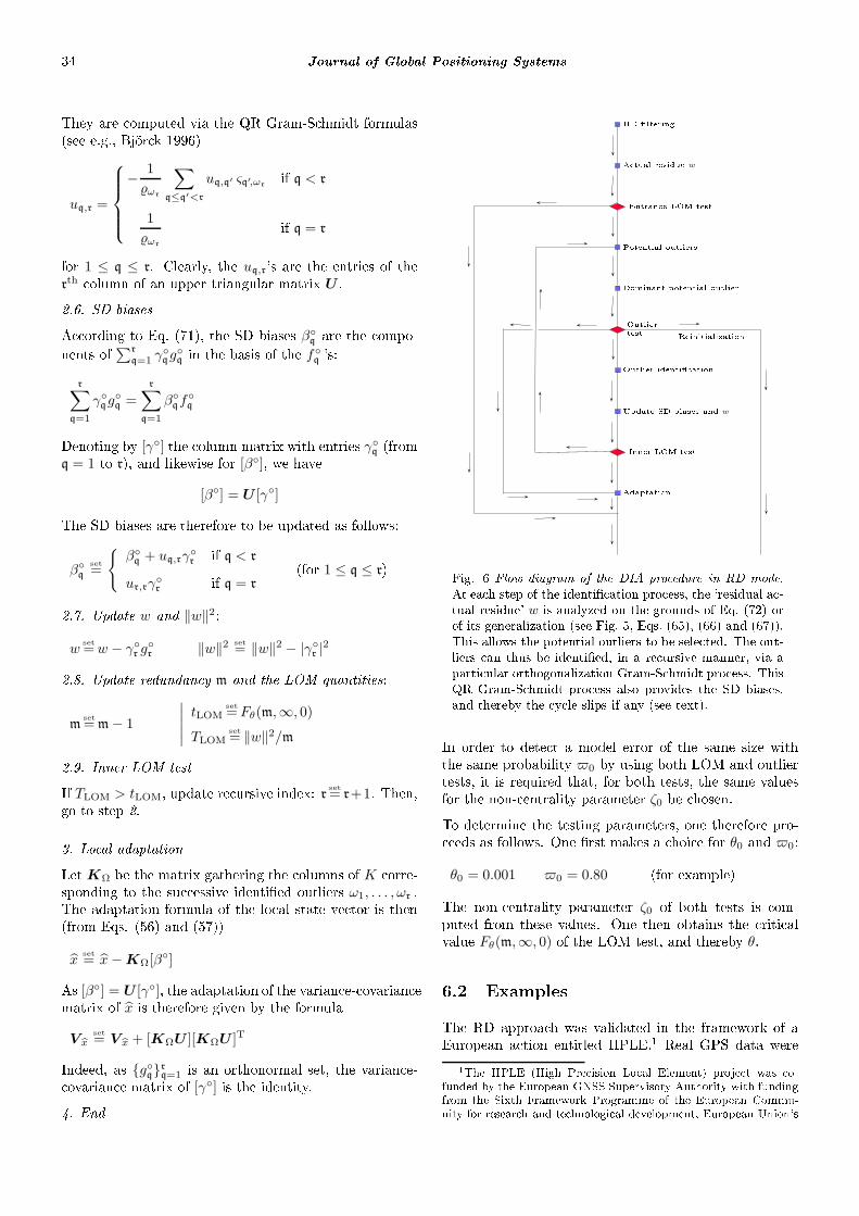
34 Journal of Global Positioning SystemsThey are omputed via the QR Gram-S hmidt formulas(see e.g., Björ k 1996)uq,r =

−1

ωr

∑

q≤q′<r

uq,q′ ςq′,ωrif q < r

1

ωr

if q = rfor 1 ≤ q ≤ r. Clearly, the uq,r's are the entries of therth olumn of an upper triangular matrix U .2.6. SD biasesA ording to Eq. (71), the SD biases β

q are the ompo-nents of ∑r

q=1 γqg

qin the basis of the f

q's:

r∑

q=1

γqgq =

r∑

q=1

βqf

qDenoting by [γ] the olumn matrix with entries γq (from

q = 1 to r), and likewise for [β], we have[β] = U [γ]The SD biases are therefore to be updated as follows:

βq

set

=

β

q+ uq,rγ

r

if q < r

ur,rγr

if q = r

(for 1 ≤ q ≤ r)2.7. Update w and ‖w‖2:w

set

=w − γr gr ‖w‖2

set

= ‖w‖2 − |γr |22.8. Update redundan y m and the LOM quantities:

mset

= m− 1

∣∣∣∣∣tLOM

set

= Fθ(m,∞, 0)

TLOMset

= ‖w‖2/m2.9. Inner LOM testIf TLOM > tLOM, update re ursive index: rset

= r+1. Then,go to step 2.3. Lo al adaptationLet KΩ be the matrix gathering the olumns of K orre-sponding to the su essive identied outliers ω1, . . . , ωr .The adaptation formula of the lo al state ve tor is then(from Eqs. (56) and (57))x

set

= x−KΩ[β]As [β] = U [γ], the adaptation of the varian e- ovarian ematrix of x is therefore given by the formulaV bx

set

= V bx + [KΩU ][KΩU ]TIndeed, as gqrq=1 is an orthonormal set, the varian e- ovarian e matrix of [γ] is the identity.4. End

RD lteringA tual residue wEntran e LOM testPotential outliersDominant potential outlierOutliertestOutlier identi ationUpdate SD biases and wInner LOM testAdaptationReinitialization

Fig. 6 Flow diagram of the DIA pro edure in RD mode.At ea h step of the identi ation pro ess, the `residual a -tual residue' w is analyzed on the grounds of Eq. (72) orof its generalization (see Fig. 5, Eqs. (65), (66) and (67)).This allows the potential outliers to be sele ted. The out-liers an thus be identied, in a re ursive manner, via aparti ular orthogonalization Gram-S hmidt pro ess. ThisQR Gram-S hmidt pro ess also provides the SD biases,and thereby the y le slips if any (see text).In order to dete t a model error of the same size withthe same probability 0 by using both LOM and outliertests, it is required that, for both tests, the same valuesfor the non- entrality parameter ζ0 be hosen.To determine the testing parameters, one therefore pro- eeds as follows. One rst makes a hoi e for θ0 and 0:θ0 = 0.001 0 = 0.80 (for example)The non- entrality parameter ζ0 of both tests is om-puted from these values. One then obtains the riti alvalue Fθ(m,∞, 0) of the LOM test, and thereby θ.6.2 ExamplesThe RD approa h was validated in the framework of aEuropean a tion entitled HPLE.1 Real GPS data were1The HPLE (High Pre ision Lo al Element) proje t was o-funded by the European GNSS Supervisory Authority with fundingfrom the Sixth Framework Programme of the European Commu-nity for resear h and te hnologi al development, European Union's

Lannes: Dierential GPS The redu ed dieren e approa h 35thus pro essed in the dual and single-frequen y modes.For all these data sets, the DIA pro edure was ondu tedwith ηj = 2 for all j.In the single-frequen y mode, Equation (65) then redu esto‖w‖2 =

1

2σ2p

n∑

j=1

|wjp|2 +

1

2σ2φ

n∑

j=1

|wjφ|2 (72)As a general rule, at ea h step of the re ursive identi- ation pro ess, the jp or jφ to be sele ted, the dominantpotential outlier, then orresponds to the maximal valueof |wjp|/σp and |wjφ|/σφ for j = 1, . . . , n (see Fig. 5). Asillustrated in the following examples, this is also the asein dual-frequen y mode.We now present related results on erning a set of GPSdata provided by the Fren h DGA for testing: 4907 epo hsat 1Hz in dual-frequen y mode (L1-C/A, L2-P) with manyappearan es and disappearan es of satellites. Over thistime series, depending on the epo hs, their number was7, 8 or 9.The referen e and user re eivers were stati . The rela-tive Cartesian oordinates of the user re eiver were of theorder of −303m, 121m and 238m.The data set in question was reinitialized at the followingepo hs: 1094, 1301, 3010 and 4689. The ambiguities werethen xed in one or two se onds: the position of the userre eiver was thus retrieved, up to one entimeter, ex eptfor epo hs 1, 1094, 13011302, 30103011 and 4689-4690.Table 1 Dual-frequen y DD ambigui-ties a

j

fν ; k for j = 1, . . . , n with n =

9 and k = 1. At the epo h under onsideration, these ambiguities werexed; for their RD trans ription, seetext (and Se t. 5.2, in parti ular).j; fν f1 f2

1 0 0

2 34 868 257 496

3 625 263 −196 104

4 −2 502 896 −1 419 324

5 12 155 323 9 705 967

6 −2 593 167 −1 303 294

7 5 973 773 4 346 092

8 9 056 740 7 252 801

9 −9 386 838 −7 332 507To illustrate the dual-frequen y version of the approa hpresented in this paper, we now on entrate on the pro- hief instrument for funding resear h. The European GNSS Super-visory Authority is the EC agen y in harge of the implementationof Galileo, Europe's future satellite navigation system.

ess at epo h 4745. Nine satellites were then available:satellites 1, 5, 7, 8, 9, 21, 23, 26, 30 (j = 1, . . . , 9).At that epo h, the ambiguity ve tor (af1 , af2) was xed.The DD trans ription of its omponents is displayed inTable 1 for k = 1.For j = 1, . . . , n, and for ea h frequen y, the orrespond-ing RD ambiguities are then given by Eq. (62) with k = 1,α

set

= af1 and αset

= af2 . It was of ourse veried thatthe estimated relative oordinates of the user re eiverwere exa tly the same in both approa hes: −303.39m,120.92m and 238.49m (the orre t values up to one en-timeter).The DIA pro edure implemented in that ase was the FLSdual-frequen y version of that presented in Se tion 6.1.The following two situations were then onsidered:A. Without any y le slip (the real data)B. With the following added y le slips (just to showthe e ien y of the method):

• 2 y les in the re eption of the f1-signal om-ing from satellite 5 (j = 2);• −1 y le in the re eption of the f2-signal om-ing from satellite 8 (j = 4);A. Dete tion and identi ation without any y le slipIn that ase, the entran e value of TLOM (9.13) was greaterthan the orresponding value of tLOM (1.26). The outlierswere then identied in the following order:Outlier TLOM

(f2 ; 1p) 5.40

(f1 ; 4φ) 2.63

(f1 ; 1p) 1.63

(f1 ; 8p) 1.06The value in the right-hand side olumn is the orre-sponding redu ed value of TLOM . The last value of TLOM(1.06) is smaller than the orresponding value of tLOM(1.30). The biases thus found are displayed in Table 2.B. Dete tion and identi ation with y le slipsThe entran e value of TLOM was then very large (335.09),mu h greater than the orresponding value of tLOM (1.26).The outliers were then identied in the following order:Outlier TLOM

(f1 ; 2φ) 108.81

(f2 ; 4φ) 9.42

(f2 ; 1p) 5.41

(f1 ; 4φ) 2.82

(f1 ; 1p) 1.74

(f1 ; 8p) 1.13

36 Journal of Global Positioning SystemsThe last value of TLOM (1.13) is smaller than the orre-sponding value of tLOM (1.34). The biases thus found aredisplayed in Table 3.All over the time series under onsideration, the resultswere the same with κ = 1 or κ = 0 (see step 2.1 and Fig. 5in Se t. 6.1). It is important to note that the hoi eκ = 0, whi h indu es some CPU overhead (see step 2.2in Se t. 6.1), impli itly orresponds the DD implementa-tion of the DIA pro edure by the Teunissen group at theTe hni al University of Delft (TUD). In Kalman mode,κ should likely be set equal to a smaller value (say 0.5 asin Fig. 5). This point remains to be investigated.Table 2 Identi ation of a set of SD biases. Thebiases βfν ;jψ are expressed in meters. At theepo h under onsideration, nine satellites wereavailable: n = 9 (see text).Frequen y f1

jψ 1 2 4 8p − 4.806 −3.304

φ 0.043Frequen y f2

jψ 1 2 4 8p − 8.755Table 3 Identi ation of a set of SD biases in lud-ing y le slips. The situation is the same as thatdened in Table 2, but with added y le slips.The latter are orre tly retrieved: βf1;2φ ≃ 2λ1 ,

βf2;4φ ≃ −λ2 . Note that the identi ation orderis, rst, that indu ed by the y le slips, and then,that displayed in ase A (see text and Table 2).Frequen y f1

jψ 1 2 4 8p − 4.806 −3.304

φ 0.381 0.043Frequen y f2

jψ 1 2 4 8p − 8.755

φ −0.2487 Con luding ommentsThe verti es of a GNSS graph are the re eivers and thesatellites of the GNSS devi e (see Lannes and Durand2003). Its edges are the re eiver-satellite pairs. The origi-nal observations are dened on these edges (see Se t. 2.1).As these observations are dened up to ve tors in thenuisan e delay spa e (see Se t. 2.1.1 and Fig. 4), the or-thogonal omplement of this spa e in the observational

data spa e plays a key part in the data assimilation pro- edures. In parti ular, brought ba k to this orthogonal omplement, the residual quantities to be onsidered inthe DIA pro edures take their values on the edges ofthe graph.To stress what is essential, the analysis presented in thispaper was restri ted to the spe ial ase where the GNSSgraph in ludes only two re eivers. On the two edges in-volved in the denition of a single dieren e, the double entralized observations of Shi and Han (1992) are thenopposite. As laried in Se t. 1.1.5, the information on-tained in these observations is then a simple antisymmet-ri trans ription of that ontained in the RD data.The DD and RD approa hes prove to be equivalent. Morepre isely, as spe ied in Se t. 3, the hoi e of the ref-eren e satellite indu es that of a referen e basis of theRD data spa e. The omponents of a RD ve tor in thisbasis are the orresponding DD's. Solving the problemin DD mode therefore amounts to solving it in this basis.At any stage of the data assimilation pro edure, one maytherefore pass from the RD mode to the DD mode, andvi e-versa. In parti ular, solving the rational-ambiguityproblem of the RD mode amounts to solving a nearest-latti e-point problem of DD type (see Se t. 5.2).In RD mode, all the satellites are handled in the samemanner. As a result, the numeri al odes of the RD dataassimilation pro esses are more readable than those oftheir DD versions. For example, in RD mode, the disap-pearan e of the referen e satellite of the DD approa h ishandled like that of any satellite.This said, the main interest of the RD approa h lies inthe properties revealed by the orresponding `dual anal-ysis' (see Se t. 4). These properties, whi h are maskedin the DD approa h (see Remark 4.2.2), shed a new lighton the CO approa h of Shi and Han (1992). In parti u-lar, Result 4.2.2 an be exploited in the DIA pro edures.From this point of view, Equation (43) is very signi ant.The notion of potential outlier derives from its orollary,the Eu lidean quadrati de omposition (44); see Fig. 5.These properties also omplete the ontribution of Lannesand Durand (2003). All these aspe ts are analyzed and ommented in Remark 4.2.1. As a result, all these equiv-alent approa hes an benet from ea h other.The DIA pro edure des ribed in Se tion 6 follows themain guidelines of the DIA method of the TUD group(see, e.g., Fig. 6 in Teunissen 1990). In parti ular, there ursive dete tion pro ess is based on a Gram-S hmidtorthogonalization pro edure. The main new points de-rive from the notion of potential outliers. The orthogo-nalization pro edure was implemented a ordingly. Thee ien y of the DIA method is thus improved. This par-ti ular implementation also benets from the QR Gram-S hmidt step 2.5 of Se t. 6.1. The QR approa h of thePhD dissertation of Tiberius (1998) an thereby be ni ely ompleted. As spe ied in step 2.6 of Se t. 6.1, the SD bi-ases an thus be re ursively rened. The identi ation of

Lannes: Dierential GPS The redu ed dieren e approa h 37 y le slips, in parti ular, is performed in this way (seeTable 3).The GNSS graph may in lude more than two re eivers;some re eiver-satellite edges may also be missing. In thisgeneral situation, that of GNSS networks with missingdata, it is important to benet from all the redundan yof the data. The ìdentiable biases' must then be iden-tied on the edges (or pairs of edges) where they ap-pear. To solve the related problems in an e ient man-ner, the DD and CO approa hes have to be onjugatedand generalized in the `proje ted observational frame-work' of Fig. 4. The related developments will be pre-sented in a forth oming paper (Lannes 2008).Referen esAgrell E., Eriksson T., Vardy A. and Zeger K. (2002)Closest point sear h in latti es. IEEE Trans. In-form. Theory. 48: 22012214.Björ k A. (1996) Numeri al methods for least-squaresproblems. SIAM.Hewitson S., Lee H.K. and Wang J. (2004) Lo alizabil-ity analysis for GPS/Galileo re eiver autonomousintegrity monitoring . The Journal of Navigation,Royal Institute of Navigation 57: 245259.

Lannes A. and Durand S. (2003) Dual algebrai formu-lation of dierential GPS . J. Geod. 77: 2229.Lannes A. (2008) GNSS networks with missing data:identiable biases and potential outliers. Pro .ENC GNSS-2008. Toulouse, Fran e.Shi P. H. and Han S. (1992) Centralized undierentialmethod for GPS network adjustment . AustralianJournal of Geodesy, Photogrammetry and Surveying.57: 89-100.Strang G. and Borre K. (1997) Linear algebra, geodesy,and GPS , Wellesley-Cambridge Press, Massa hus-sets.Teunissen P.J.G. (1990) An integrity and quality ontrol pro edure for use in multi sensor integra-tion . Pro . ION GPS-90. Colorado Springs, Col-orado USA: 513-522Teunissen P.J.G. (1995) The least-squares ambiguityde orrelation adjustment: a method for fast GPSinteger ambiguity estimation . J. Geod. 70: 6582.Tiberius C.C.J.M. (1998) Re ursive data pro essing forkinemati GPS surveying . Publi ations on Geodesy.New series: ISSN 0165 1706, Number 45. NetherlandsGeodeti Commission, Delft.


A Robust Indoor Positioning and Auto-Localisation Algorithm

Rainer Mautz Institute of Geodesy and Photogrammetry,Swiss Federal Institute of Technology, ETH Zurich Washington Y. Ochieng Centre for Transport Studies, Department of Civil and Environmental Engineering, Imperial College London, London, United Kingdom, SW7 2AZ Abstract. Sensor networks that use wireless technology (IEEE standards) to measure distances between network nodes allow 3D positioning and real-time tracking of devices in environments where Global Navigation Satellite Systems (GNSS) have no coverage. Such a system requires three key capabilities: extraction of ranges between sensor nodes, appropriate supporting network communications and positioning. Recent research has shown that the first two of these capabilities are feasible. This paper builds on this and develops an automatic and robust 3D positioning capability. A strategy is presented that enables high integrity positioning even in the presence of large mean errors in the range measurements. This is achieved by an algorithm that generates a tight, high-confidence upper bound on the error in a position estimate, given the noisy range measurements from the radio devices in view. As a core feature, we present a novel network auto-localisation algorithm that fully automatically determines the positions of all nearby fixed nodes. Results from a real network using the Cricket Indoor Location System show how all sensor nodes can be determined based on only one dynamic node. Simulations of static networks with 100 nodes demonstrate the importance of solving folding ambiguities. Studies from networks with imprecise range measurements have shown that it is possible to theoretically achieve a position deviation that is of the size of the ranging error.

Keywords. auto-localisation, positioning algorithm, wireless sensor positioning, multilateration

1 Introduction

1.1 Background

Despite Global Navigation Satellite Systems (GNSS) being the most pervasive positioning systems, alternative and complementary systems are essential because GNSS are unsuitable for some ad-hoc sensor network operational environments. In particular, they cannot work indoors or in the presence of obstacles that block the signals from the GNSS satellites. This is commonly addressed by combining or integrating GPS with deduced reckoning (DR) sensors including inertial navigation systems (INS). DR, with the aid of a gyroscope and odometer, is commonly used to bridge any gaps in GPS positioning, but its positioning error grows rapidly if not controlled by other sensors or systems such as GPS. The use of cellular communications networks to assist GPS receivers in difficult environments is referred to as Assisted Global Positioning Services (A-GPS), where GPS is integrated in a mobile network and the processing is partly taken over by the network. According to Darnell and Wilczoch (2002) positioning accuracy of 50m indoors can be reached with A-GPS. The system proposed in this paper however is designed to reach a decimetre to centimetre accuracy (2 σ) indoors.

The limitations of GNSS have motivated the search for complementary methods in addition to those above. Recently, a large number of wireless positioning systems has been proposed and evaluated, e.g. Niculescu and Nath (2001), Savarese et al. (2002), Savvides et al. (2003) and Smith et al. (2004). Network positioning based on graph theory has been investigated extensively using a set of range measurements between network nodes, e.g. by Eren et al. (2004) and Goldenberg et al. (2005). Wireless devices enjoy widespread use in numerous diverse applications including sensor networks. The exciting new field of wireless sensor networks breaks away from the traditional end-to-end communication of voice and data

Mautz and Ochieng: A Robust Indoor Positioning and Auto-Localisation Algorithm 39

systems, and introduces a new form of distributed information exchange. The near future scenario consists of countless tiny embedded devices, equipped with sensing capabilities, deployed in all environments and organising themselves in an ad-hoc fashion.

Knowing the correct positions of network nodes is essential to many applications in future pervasive sensor networks. Examples include usage in crime prevention, emergency and incidence respond management, product tracking at industrial sites, wildlife habitat monitoring and home control. Further applications are user guidance, efficient routing in communication networks, detection of unauthorised removal of assets and geofencing.

However, for many applications, the integrity of the location information yielded from such a wireless sensor network is vital. The research focus has been on the determination of positions, effectively ignoring measurement noise. Little attention has been given to the fact that range observations are corrupted by gross errors and also affected by measurement noise. Additionally, the correctness of the coordinate positions of anchor nodes, which ‘know’ their positions cannot be taken for granted for real world scenarios. All these different error sources can lead to inaccurate position information. This paper takes these errors into account. A wireless positioning system which is used for Safety of Life (SoL) or liability critical applications is required to be of high reliability and integrity. It is not sufficient to deliver a coordinate output, even with corresponding figures of the uncertainties (in terms of a variance-covariance matrix). In fact, a rigorous validation process must provide the user with reliable and complete integrity information for the positional data. Any partial or complete system failure needs to be forwarded immediately to the user, who is then able to rely on the system status as indicated by the system itself.

1.2 The used wireless sensor platform

The system that has been used for the experiments in this paper in order to obtain ranging data for positioning and tracking is called Cricket. The Cricket nodes are tiny devices developed by the MIT Laboratory for Computer Science as part of the Project Oxygen, details are given in Priyantha (2005). A Cricket board is shown in Fig. 1. A deployed Cricket location sensing infrastructure enables people or devices to determine their position while indoors. The Cricket unit can be programmed as either as a beacon or listener. The beacons are typically static units that are mounted on the ceiling above the mobile listeners. The beacon unit broadcasts periodically an ultrasonic (US) pulse and at the same time a radio frequency (RF) message with its unique ID number. Using the time-of-flight information from different beacons and the temperature corrected speed of sound

measurement; the listener calculates its distance from the beacons. Because RF travels about 106 times faster than ultrasound, the listener can use the time difference of arrival between the start of the RF message from a beacon and the corresponding ultrasonic pulse to infer its distance from the beacon. The position of the listener can then be determined based on the beacon node positions and the measured ranges.

Fig. 1. Cricket unit / RS232 cable assembly

One reason to choose the Cricket system as a test bed for the novel positioning algorithm was its flexibility and programmability. For example, Cricket listeners and beacons consist of identical hardware. Even the software that is running on listeners and beacons can be the same – a simple command from the host can change a Cricket node from a listener into a beacon and vice versa. The embedded software that is running on a Cricket device can be replaced simply by uploading the flash memory with modified or self-developed programs. The open architecture of Crickets has inspired researchers all over the world to use Cricket as a platform to develop new wireless positioning strategies and for algorithm testing. There is plenty of literature on Crickets and applications available. The thesis of Priyantha (2005) describes the design and implementation of the Cricket indoor location system in detail. Haggag and Mehraei (2006) document their modification of the default architecture that enables coordinated robot interaction. Wang (2004) lays the foundations for leveraging the Cricket indoor location system to supply orientation information. He also demonstrates end-to-end functionality of a Cricket Compass.

However, there are several disadvantages when choosing Cricket as a platform for ranging and positioning. In order to obtain ranges between motes, the time of flight between an ultrasonic pulse and a radio signal needs to be measured. Both, the US pulse and the RF signal sometimes suffer from multipath effects, in particular indoors due to reflections at walls, windows, tables or the floor. When a listener receives a reflected signal instead of the direct signal along the line-of-sight, a too long range is determined. A multipath signal is particularly likely to occur when a beacon node is not orientated towards the listener. Typically a listener unit can detect ultrasonic signals from a beacon within a 40 degree cone. If the beacon node is not orientated directly towards a


listener, the listener receives a reflected signal instead of the direct signal. Fig. 2 shows such a scenario, where a multipath signal is received. In order to eliminate a gross error due to multipath, a high redundancy of range measurements (i.e. more than 5 ranges to each node) is necessary.

Fig. 2. Multipath scenario where the signal is reflected at the ceiling

There are several more disadvantages associated with the use of ultrasound. The speed of ultrasound is highly correlated to the temperature. Although cricket units carry temperature sensors on their chip sets, it is hard to obtain an accurate temperature along the path between sender and receiver. The speed of ultrasound depends tightly on the speed of wind, which doesn’t allow for accurate positioning outdoors. With the ultrasound sender not transmitting omni-directionally, it is almost impossible to set up a dense ad-hoc network with a large number of Cricket units. In a large ad-hoc sensor network the condition that the nodes face each other is normally not fulfilled. Taylor (2005) and Taylor et al. (2006) modified a mobile cricket by attaching two additional ultrasound transducers. These transducers more closely simulate an omni-directional acoustic pulse than the conic emanation of the standard cricket transducer. His positioning algorithm uses range measurements between sensors and a moving target to simultaneously localize the sensors, calibrate sensing hardware, and recover the target's trajectory. In his experiments he used up to 55 sensors to cover a 7 x 10 meter room. Our auto-localisation algorithm however uses a lower number of beacon nodes to perform localisation and tracking.

Our local 3D positioning algorithm takes into account the weaknesses of current wireless ad-hoc positioning methods and algorithms, including the absence of quality and integrity indicators for the positioning results, existence of high variances and outliers in range measurements, errors in anchor nodes (or even their absence) as well as a coarse positioning mode for poorly conditioned networks.

2 Positioning

Our contribution to positioning addresses two different network computation methods. While the first section

describes a method to obtain the node positions with one mobile node the second section uses inter-beacon range measurements to create a geodetic network that allows position determination.

2 Obtaining beacon coordinates by auto-localisation

Auto-localisation is also known as Mobile Assisted Positioning or SLAT (Simultaneous Localization and Tracking) and refers to the problem to obtain the coor-dinate positions of fixed anchor nodes which are required to enable tracking of mobile devices. Without the use of an auto-localisation algorithm the coordinates of the fixed beacon node positions would have to be determined with another positioning system. Because GNSS is not avail-able indoors and because the quality of the beacon nodes should be at least as good as the wireless positioning system (if not a magnitude better), time-consuming manual positioning methods are usually required to obtain beacon coordinates. Typically tachymeter measurements are carried out with a positioning accuracy of 5-10 mm (1 sigma). However, it is not practical to use a second positioning system to calibrate the beacon nodes because that increases time and effort.

The auto-location strategy used for positioning of the beacon nodes is shown in Fig. 3. A dynamic listener is slowly moved at different locations in a room thereby collecting ranging data to 4 (or more) beacon nodes that are mounted at the ceiling. Both, the mobile and the static node positions are unknown. Even the inter-beacon ranges are not available. This is the most challenging scenario for an auto-localisation task, but nevertheless the most likely scenario to occur after the nodes have been deployed in a room. The described scenario still allows creating a rigid network based on local coordinates. The deployment of static nodes in the four corners of a room allows the set up of a meaningful local coordinate system orientated along the four orthogonal walls.

Fig. 3. Auto-localisation of beacon nodes by a mobile node

Generally, the redundancy of the auto-localisation problem in 3D is given by

,6)(3redundancy ++−= PBR (1)

Ceiling

Beacons (static)

Ceiling

Floor Beacon Listener

Ceiling


where R is the number of observed ranges, B the number of fixed beacons and P the number of listener positions. If the direct line of sight conditions allow to obtain all combinations of ranges, then R = B P holds. In Fig. 3, the mobile listener has collected 4 ranges to 4 beacons at 6 different locations. Assuming the 3D case, there are 3(B + P) = 30 unknown coordinates and B P = 24 range measurements. Taking into account the 6 degrees of freedom for a free 3D network, a solution would theoretically be possible without any redundancy. However, our results show that a zero or a low redundancy of the network causes the auto-localisation algorithm to fail under real field conditions. Due to the existence of outlier observations, bad geometric constraints and linearization errors of the objective function large errors in the position estimation are likely to occur. This is particularly the case in scenarios with a small redundancy, large mean or gross errors in the range measurements. In order to obtain the beacon coordinates the following procedure had been carried out:

a) Stepwise movement of the listener in a room while collecting range measurements.

b) Grouping of the ranges into P listener positions according to their time stamps.

c) Detection of gross errors by comparing timely nearby ranges and testing triangle conditions.

d) Setting up a distance matrix R between all nodes of the network with size (B + P) by (B + P), see Fig. 4.

e) Filling the gaps of the distance-matrix using a simple interpolation scheme. This step establishes rough approximation of all inter-nodal ranges.

f) Setting up a local coordinate system based on the inter-nodal ranges of four nodes (preferably beacon nodes).

g) Computation of all coordinate positions based on multidimensional scaling (MDS), a localisation method that transforms proximity information into geometric embedding. Details of the algorithm can be found in Shang et al. (2004). Alternatively, the positions can be determined by multilateration from four locally defined nodes. Our experiments have shown that this alternative has better performance than MDS.

h) Refinement of the coordinates by geodetic network adjustment. In application on real data this step can usually not be carried out straight away. The reason is that network adjustment involves linearization of the objective function, which is eligible only if of good approximate values of the unknowns are available. Here, the initial approximate positions are not precise enough to directly apply network adjustment using the Gauss-Newton iteration. In order to avoid a failure of the network adjustment, a heuristic optimisation method is carried out that directly uses the non-linear objective function. Using trial and error the coordinate positions are shifted in order to fit the range

measurements. The heuristic step improves approxi-mate positions for the network adjustment – typically from meter to cm level. The disadvantage of using heuristic methods is the high computational cost. However, taking into account that the auto-localisation is executed only once and not processed in real-time, the usage of timely expensive heuristic methods is not critical. An insight into heuristic methods is given in Mautz (2002).

B1 B2 B3 B4 P1 P2 P3 P4 P5 P6

B1

B2 not observed observed

B3

B4

P1

P2

P3 observed not observed

P4

P5

P6 Fig. 4. Distance matrix of the example with 4 beacons and 6 listener

positions

After the auto-localisation procedure has been completed, the coordinates of the static beacon nodes are available in a local system. An over-determined auto-location setup allows determining quality indicators of the coordinates. A numerical example based on mobile assisted positioning is given in the experimental results section.

2.2 Instant coordinate determination in a sense network

In case the network has an inter-nodal connectivity of c > 4 (or c > 3 in 2D), the network can be initialised without a multi-epochal auto-localisation procedure. Once the ranges between the beacons have been obtained and collected at a central processing unit, the sensor position coordinates can be determined based on only a single epoch. Thereby it does not matter, whether the nodes are static or dynamic. The positioning strategy is based on the creation of a rigid structure: The key issue for an anchor free positioning is to find a globally rigid graph, or in other words, a structure of nodes and ranges which has only one unique embedding, but still can be rotated, translated and reflected. In 3D, the smallest graph consists of five fully connected nodes in general position. If such an initial cluster passes statistical tests, additional vertices are added consecutively using a verified


multilateration technique. Nodes that have not been able to take part in the rigid cluster are positioned using a more error prone method and thereafter added to the cluster. The process flow of our positioning strategy is illustrated in Fig. 5.

The creation of a cluster aims to compute unique positions of vertices in a local coordinate system that can be transformed into a higher spatial reference system by translations, rotations and a reflection. A straightforward method to determine the position of an object based on simultaneous range measurements from three stations located at known sites is called trilateration. Manolakis (1996) and Thomas and Ros (2005) provide fast algebraic and numeric algorithms for trilateration in robotics. Coope (2000) shows that the effect of errors in the range measurements can be particularly severe when the trilaterated point is located close the base plane or the three known stations are nearly aligned. Moore et al. (2004) show that there is a high probability of incorrect realisations of a 2D-graph when the measurements are noisy.

The coordinate system of the cluster is conveniently defined in local coordinates based on the three ranges r12, r13, r23 between the nodes P1, P2, P3. The coordinates read

( ) ( )

.0,2

,2

:

,0,0,: ,0,0,0:2

12

223

213

2122

1312

223

213

212

3

1221

⎟⎟⎟

⎠

⎞

⎜⎜⎜

⎝

⎛

⎟⎟⎠

⎞⎜⎜⎝

⎛ −+−

−+r

rrrrr

rrrP

rPP (2)

A forth point is added to the network by 3D-tilateration thereby arbitrarily choosing one of the two folding ambiguities and discarding the other. However, as long as there are only 4 points involved, the flip ambiguity does not affect the inner structure of the general tetrahedron which is spanned by the base plane and the trilaterated point. As soon as a 5th node is added to the cluster by trilateration from the points in the base plane 1, 2 and 3, the ambiguity problem does matter, as there are two different embeddings. As shown in Fig. 6, nodes 4 and 5 could be on either the same side of the base plane or on opposite sides. If the distance between nodes 4 and 5 is also measured, we call this graph a ‘quintilateral’ or in short a ‘quint’ since all 5 nodes are fully linked by range measurements to each other. Only the additional range measurement r45 between nodes 4 and 5 can disambiguate between these two embeddings. As can be seen in the example in Fig. 6, r45 is significantly longer than the reflected case r45’, which means that if r45 is available, the correct embedding can be selected. Consequently, such a quint is rigid in 3D, assuming the nodes are not in a singular position.

Fig. 5. Positioning algorithm, which does not require any initial

approximate coordinates

However, there are geometric constellations where the ambiguity cannot be solved by the redundant range r45, because the difference between the distances d45 and d45’ is of the same magnitude as the ranging error. In order to decide which of the two embeddings is correct, we compare the computed distances d45 and d45’ with the measured distance r45. In some cases the differences between the measured and the calculated distances Δ45 = |r45 - d45| and Δ45’ = |r45 - d45’| may both be very small. Assuming a mean error of the range measurement r45, say 5%, both differences Δ45 and Δ45’ are likely to pass the statistical test of their null hypotheses, which means that both could be a result of noise. Consequently, the range r45 does not disambiguate between both embeddings.

The best way to deal with this problem is to reject such unstable point formations. It is better not to use a non-

1. Creation of a quint

find 5 fully connected nodes

free LS adjustment

return refined coordinates and standard variations

return local coordinates

failed

no

input ranges

input anchor nodes

yes

volume test

ambiguity test

assign local coordinates

Expansion of minimal structure (iterative multilateration)

Merging of clusters (6-Parameter Transformation)

Transformation into a reference system

anchor nodes available?

failed

achieved

achieved

2. Transformation


robust quint than rely on a structure with incorrect internal flips. In our point of view it is crucial to ensure a correct embedding for several reasons. Firstly, the displacement caused by an incorrect flip can be large. Secondly, these errors have a negative affect on the expansion of the structure when additional vertices are added later. Thirdly, and most importantly, once a folding error has been introduced in a network it is hard to detect and eliminate it later.

Fig. 6. (a) Quintilateral, (b) a version where node 5 has been mirrored at

the base plane

After the quint is verified to be robust and not affected by a false flip, the next task is the expansion of the minimal rigid structure. The remaining nodes are added to the quintilateral individually using 3D-multilateration from four or more stations at a time. ‘Multilateration’ is basically a trilateration technique, where the new node is initially determined from three stations at a time. The redundant distance measurements are used to disambiguate between two different embeddings and to verify the initial computation. Multilateration allows redundant determination of the nodes. The resulting coordinate differences provide essential information to detect false range measurements, e.g. due to multipath effects.

However, there is again a high probability of incorrect folding of a graph when the measurements are noisy. For instance, if a new node is multilaterated from points located closely to one plane and the ranges are affected by errors, a flip ambiguity may occur due to the mirroring effect of that plane. These incorrect graph realisations need to be avoided by identifying weak tetrahedrons with volumes smaller than a threshold which is driven by the estimated noise in the ranges. Only tetrahedrons that have passed the test on robustness are further considered or otherwise discarded. This step again eliminates the mirroring ambiguity of nodes added to a rigid structure and improves the accuracy measures. Once a node’s position is determined, it serves as an anchor point for the determination of further unknown nodes. This way, starting from the initial quintilateral the position

information iteratively spreads through the whole network.

The trilateration and multilateration problem considered so far solves for one single unknown point at a time. The sequential accumulation of nodes by multilateration is known as iterative multilateration (Savvides, 2001). However, this technique is very sensitive to measurement noise. Initially, small errors accumulate quickly while expanding the network. The propagation of errors in a large network must be minimised as much as possible. Geodetic network adjustment is an essential tool to evenly distribute the errors that have been accumulated by iterative multilateration. Network adjustment provides coordinate estimates of several unknown nodes thereby improving the reliability of the quality indicators as determined a posteriori, see Grafarend and Sanso (1985). The theory of linear Least-Squares (LS) adjustment can be found in Grafarend and Schaffrin (1993).

Outlier observations distort the network but they cannot be isolated by performing a least-squares adjustment and analysing the residuals. Thus, outliers need to be removed in a separate analysis before the network is adjusted. While performing simulations on the anchor free start-up, results show that only a fraction of vertices can become a member of one single cluster. The remaining vertices are likely to make up their own clusters which may or may not be connected to neighbouring clusters. In case two clusters share a sufficient number of vertices and/or range observations between them, they can be merged using an over-determined 3 dimensional 6-parameter transfor-mation.

The outcome of clusterisation is a cluster of nodes with their coordinates and variances in a local system. As this step is concluded by a free minimally-constrained least-squares adjustment it is possible to assess the internal consistency of the measurements.

A more elaborate discussion of the positioning algorithm and details of the mathematical background are presented in Mautz et al. (2007).

2.3 Transformation into a reference coordinate system

Most applications require the network nodes to be tied in a coordinate system of higher order. With a minimum availability of four anchor nodes, the local coordinates can be transformed unambiguously into the relevant target system. This can be achieved by a 3D-Cartesian coordinate transformation. A closed form solution for the determination of transformation parameters using the 3D-Helmert transformation is given by Horn (1987). Subsequent to the transformation, a fully constraint LS network adjustment is performed that permits all of the available anchor nodes and all range measurements to be processed together in order to refine all position

1

3 2

4

5

1

3 2

4

5’

(a) (b)


approximates simultaneously. Additionally, the mean error in the coordinates is reported by the point confidence ellipse for each node.

3 Experimental Results

In section 3.1 the performance of the localisation algorithm proposed in chapter 2 is evaluated on real sensor data obtained from Cricket nodes. In order to asses the performance of a large and dense network simulated ranging data are used in section 3.2.

3.1 Initialisation of a dynamic network

In order to assess the performance of network initialisation with the support of a mobile node (with unknown positions!), the following measurement setup was chosen: four stationary nodes (= beacon nodes) were deployed at the office ceiling. Due to the system architecture of crickets the inter-beacon range signals could be obtained. One dynamic node was carried through the room and range measurements taken at an interval of 1s between the mobile node and the static nodes located in the corners. Within a time span of 5 minutes, 1000 range measurements had been obtained with a priori noise level of σr = 0.01m. Now the task for the positioning algorithm was to recover the 3D network geometry without adding any supplementary information, e.g. geometric constraints or approximate positional information. The main difficulty in recovering the relative node positions for this configuration is that the connectivity graph does not contain five nodes making up a quint. Consequently, the strategy described in section 2.2 could not be followed and the post-processing method described in 2.1 was used instead. This method included: setting up a rough distance matrix, global optimisation of the objective function and network adjustment.

In a first step, the range measurements are grouped into 34 epochs of 2.5 second intervals each by an implemented algorithm. Multiple range observations within one group are averaged if there is a difference of less than 2 cm, or discarded otherwise. 120 range measurements are finally taken into account to determine 30 virtual node positions of the dynamic node and 4 beacon node positions. Consequently, the number of unknowns is 3 * 34 = 102. According to (1) the redundancy of the system can be computed as 120 – 102 + 6 = 24. The redundant distance constraints in the network could be used to determine the system inconsistency and the empiric mean error of the node positions. After step g) in section 2.1 had been carried out, the empiric mean error was 1.52m. With application of the refinement step (global optimisation) the error could be further reduced to 0.05m and finally down to

0.0096m by network adjustment. This mean error is within the magnitude of the observational noise level. Thus, the inner network geometry could be recovered successfully. Fig. 7 shows the location of the recovered node positions.

Fig.7. X-Y view with 4 stationary cricket node positions in the corners of a room (black dots) and 30 virtual positions of a mobile node (red

dots).

This example shows that it is feasible to establish a local network in a room without surveyed anchor nodes, any presumptions on the node locations or any inter-node range measurements between the static devices. After the mobile positioning algorithm has been carried out, all distances between the static nodes are determined. The graph between the static nodes is a rigid structure that can be used for further navigation of mobile nodes.

3.2 Initialisation of a dense network

In order to assess the performance of the proposed positioning algorithm, a simulated network consisting of 100 nodes was set up randomly in a 10 m × 10 m × 10 m test cube. Assuming a maximum communication range of 3.5 m between the radios, only the inter-node distances of less than 3.5 m have been recorded into an observation file. After execution, the file contained 570 range measurements. Based on these 570 ranges, the positioning algorithm was used to recover the node po-sitions. As detailed in the section 2.2, the algorithm created quints, then larger clusters by lateration and cluster merging. 10 points were chosen randomly to serve as anchor nodes for a 3D-transformation of the local cluster into the original geodetic datum.

The criterion used for the performance assessment in positioning is the average deviation

( ) ,ˆ1

21∑=−=

n

i iinpa PP (3)

-0.5 0 0.5 1 1.5 2 2.5 30

0.5

1

1.5

2

2.5

3

3.5

4

4.5

1 2

34

5 6 7 8 9

10 11 12

131415 16

17

18 19

202122232425

26 27 28 29

30 31 32

3334

X

Y

[m]

[m]


where n is the number of nodes, iP the true position

vector and iP the estimated position vector of the localised node i. The internal consistency of the free network is assessed by the square root of the estimated reference variance

( )∑ =−− −==m

i iinmnmr rr1

23

13

1 ˆˆ vvTσ (4)

where v is the vector of residuals containing the differences between the estimated distances ir (obtained from a LS-adjustment) and the measured distances ri.

Fig. 8. True position deviations ap (pluses) for measurement noise σr between 0m and 0.2m. For comparison, the dots show the estimated deviations pa .

Fig. 9. True position deviations ap (pluses) in comparison with the

estimated reference mean errors shown as dots.

Fig. 8 shows how the noise level in the ranges σr influences the average position deviation ap of the localised nodes at a maximum signal range rmax = 3.5m. The linear dependencies on σr and ap in Figs. 8 and 9 have approximately an average proportionality factor of 1. This testifies that our localisation algorithm has almost reached the best possible performance level, which has

been determined by Savvides (2003a) as the Cramer Rao Bound behaviour. This is especially true for noise levels with less than 3.5% error (0.1m level), where almost all nodes in all networks have been localised correctly. Note that a single falsely located node (e.g. due to a false folding ambiguity) causes the average position deviation to rise significantly.

4 Conclusions

The cricket sensor node system has been used to successfully apply a full 3D auto-location algorithm. Furthermore, it could be shown that a dense network of inter-beacon ranges can be used compute an instantaneous geodetic network.

Experimentation has shown that the motion of a mobile node can be exploited to automatically create the rigid topology of the network nodes. Range measurements taken at various points in time of a mobile node have enabled positioning of all nodes in a local coordinate system. However, this auto-localisation method requires a high redundancy of observations and a full elimination of outliers in the range measurements, since the computation of coordinates is extremely sensitive to errors.

A second experiment based on simulation has demonstrated the feasibility to determine dense ad-hoc distance networks with the presence of large observation errors and poor geometric conditions. In order to achieve a reliable positioning based on geodetic adjustment even in the presence of errors and sub-optimal geometry, a robust algorithm has been set up, that particularly avoids flip ambiguities in the network. We have studied networks with relatively large measurement errors of up to 7.5% of the true ranges and shown that it is possible to achieve a position deviation that is of the size of the ranging error.

Future work will focus on further moving away from laboratory conditions. The application of the algorithms for other sensor hardware (besides the Cricket System) will be the next challenge. A major challenge will be a positioning functionality for ill-conditioned networks that makes best use of available range measurements, connectivity information, temporal-spatial derivatives, travel behaviour and GIS data.

References

Coope I (2000), Reliable computation of the points of intersection of n spheres in n-space, ANZIAM Journal, Vol. 42(E), pp. C461-477, 2000.

Darnell, C and Wilczoch, C (2002), Real Time Positioning; Construction and implementation of a GPS-Communicator. Master’s thesis in Control and

0 0.05 0.1 0.15 0.20

.05 .1 .15 .2 .25 .3 .35 .4

noise level σr [m]

mean errors rσ / deviations ap [m]

0 0.05 0.1 0.15 0.20

.05

.1

.15

.2

.25 .3

.35

.4

.45

noise level σr [m]

average deviations ap and ra [m]


Communication, Report no. LITH-ISY-EX-3246-2002, Linköping University, Sweden.

Eren, T; Goldenberg, D; Whiteley, W; Yang, Y; Morse, A; Anderson, B and Belhumeur, P (2004), Rigidity, computation and randomization of network localization. In: Proceedings of IEEE Infocom ’04, Hong Kong, China, April 2004.

Goldenberg D; Krishnamurthy, A; Maness, W; Yang, Y; Young, A; Morse, A; Savvides, A and Anderson B (2005), Network Localization in Partially Localizable Networks. In Proceedings of IEEE INFOCOM 2005, Miami, FL, March 13-17, 2005.

Grafarend, E and Sanso, F (Editors) (1985), Optimization and Design of Geodetic Networks. Springer-Verlag.

Grafarend, E and Schaffrin, B (1993), Ausgleichung in linearen Modellen, Wissenschaftsverlag, Mannheim, Leipzig, Wien Zürich

Haggag, H and Mehraei, G (2006), Robot Interaction Using Cricket, an Indoor Positioning System, Technical Report of the Maryland Engineering Research Internship Teams (MERIT), University of Maryland and Virginia Commonwealth University.

Horn, B (1987), Closed-from solution of absolute orientation using unit quaternions. Journal of Opt. Soc. Amer., vol. A-4, pp. 629–642, 1987.

Manolakis, D (1996), Efficient Solution and Performance Analysis of 3-D Position Estimation by Trilateration, IEEE Aerospace and electronic systems, Vol 32, No. 4, Oct. 1996.

Mautz, R., Ochieng, W.Y., Brodin, G., Kemp, A. (2007), 3D Wireless Network Localization from Inconsistent Distance Observations, Ad Hoc & Sensor Wireless Networks, Vol. 3, No. 2–3, pp. 141–170.

Mautz, R. (2002), Solving Nonlinear Adjustment Problems by Global Optimization, Bollettino di Geodesia e Scienze Affini, Vol. 61, No.2, pp. 123 – 134.

Moore, D; Leonard, J; Rus, D and Teller, S (2004), Robust distributed network localization with noisy range measurements, Proceedings of the ACM Symposium on Networked Embedded Systems, 2004.

Niculescu, D and Nath, B (2001), Ad-hoc positioning system, in: IEEE GlobeCom, 2001.

Priyantha N. B. (2005), The Cricket Indoor Location System, PhD Thesis, Massachusetts Institute of Technology, June 2005, 199p.

Savarese, C; Langendoen, K and Rabaey, J (2002), Robust positioning algorithms for distributed ad-hoc wireless sensor networks, in: USENIX Technical Annual Conference, Monterey, CA, 2002, pp. 317–328.

Savvides, A; Han, C and Strivastava, M (2001), Dynamic Fine-Grained Localization in Ad-hoc Networks of Sensors, Proceedings of ACM SIGMOBILE 2001, Rome, Italy, July 2001

Savvides, A; Park, H and Srivastava, M (2003), The n-Hop Multilateration Primitive for Node Localization Problems. MONET 8(4): 443-451.

Savvides, A; Garber, W; Adlakha, S; Moses, R and Srivastava, M (2003a), On the Error Characteristics of Multihop Node Localization in Ad-Hoc Sensor Networks, Proceedings of the Second International Workshop on Information Processing in Sensor Networks (IPSN'03), Palo Alto, California, 317-332.

Shang, Y; Ruml, W; Zhang, Y and Fromherz, M (2004), Localization from Connectivity in Sensor Networks, IEEE Transactions on Parallel and Distributed Systems, vol. 15, no. 11, pp. 961–974, Nov. 2004.

Smith, A; Balakrishnan, H; Goraczko, M and Priyantha N (2004), Tracking Moving Devices with the Cricket Location System, Proc. 2nd USENIX/ACM MOBISYS Conf., Boston, MA, June 2004.

Taylor, C., Rahimi, A., Bachrach, J., Shrobe, H., and Grue, A. (2006), Simultaneous localization, calibration, and tracking in an ad hoc sensor network. In: Proceedings of the 5. international Conference on information Processing in Sensor Networks (Nashville, Tennessee, USA, April 19 - 21, 2006). IPSN '06. ACM Press, New York, NY, 27-33. DOI= http://doi.acm.org/10.1145/1127777.1127785

Taylor, C J; (2005), Simultaneous Localization and Tracking in Wireless Ad-hoc Sensor Networks, Master Thesis of Engineering, Department of Electrical Engineering and Computer Science, Massachusetts Institute of Technology.

Thomas, F and Ros, L (2005), Revisiting Trilateration for Robot Localization, IEEE Transactions on Robotics, Vol. 21, No. 1, pp. 93-101, February 2005.

Wang, K J (2004), An Ultrasonic Compass for Context-Aware Mobile Applications, Master Thesis of Engineering, Department of Electrical Engineering and Computer Science, Massachusetts Institute of Technology.


Latest Developments in Network RTK Modeling to Support GNSS Modernization

Herbert Landau, Xiaoming Chen, Adrian Kipka, Ulrich Vollath Trimble Terrasat GmbH

Abstract. Global Navigation Satellite Systems like the US Global Positioning System GPS and the Russian GLONASS system are currently going through a number of modernization steps. The first satellites of the type GPS-IIR-M with L2C support were launched and from now on all new GPS satellites will transmit this new civil L2 signal. The first launch of a GPS-IIF satellite with L5 support is announced for spring 2008. Russia has started to launch GLONASS-M satellites with an extended life-time and a civil L2 signal and has announced to build up a full 18 satellite system by 2007 and a 24 satellite system by 2009. Independently of that the European Union together with the European Space Agency and other partnering countries are going to launch the new European satellite system Galileo, which will also provide worldwide satellite navigation service at some time after 2011. As a consequence we can expect to have very heterogeneous receiver hardware in these reference station networks for a transition period which could last until 2015. Network server software computing network corrections will have to deal with an increased number of signals, satellites and heterogeneity of the available data. The complexity but also the CPU load for this server software will increase dramatically. With the increasing number of signals and satellites the demands for the network server software is growing rapidly. The progress on the satellite system side is going hand in hand with the tendency of the customers to operate growing numbers of reference station receivers resulting in higher demands for CPU power. The paper presents a new approach, which allows us to process data from a large number of reference stations and multiple signals via a new federated Kalman filter approach. With the newest improvements in the GLONASS satellite system, more and more Network RTK service providers have started to use GLONASS capable receivers in their networks. Today, practically all service providers, who are using GLONASS, are applying the Virtual Reference Station (VRS) technique to deliver optimized correction streams to the users in the field. Different satellite systems and generations require different weighting in network server

processing and receiver positioning. The network correction quality depends very much on the satellite and signal type. New message types have been recently developed providing individualized statistical information for each rover on unmodeled residual geometric and ionospheric errors for GPS and GLONASS satellites. The use of this information leads to RTK performance improvements, which is demonstrated in practical examples.

Keywords: GPS, GNSS, GNSS Modernisation, Network RTK.

INTRODUCTION

After its introduction in the late 90s, Network RTK technology based on the Virtual Reference Station (VRS) approach became an accepted and proven technology, which is widely used today in a large number of installations all over the world. Developments over the past years (Chen et al., 2003, 2004, 2005; Kolb et al., 2005, Landau et al., 2002; Vollath et al., 2000, 2001) have resulted in a solution, which is marketed under the name GPSNetTM since 1999 (Vollath et al., 2000). Comparing with traditional single base RTK technology, network RTK removes a significant amount of spatially correlated errors due to the troposphere, ionosphere and satellite orbit errors, and thus allows performing RTK positioning in reference station networks with distances of 40 km or more from the next reference station while providing the performance of short baseline positioning.

Currently more than 2500 reference stations are operating in networks in more than 30 countries using the Trimble GPSNet solution. Data processing in GPSNet utilizes the mathematically optimal Kalman filter technique to process data from all network reference stations. This comprehends modelling all relevant error sources,


including satellite orbit and clock errors, reference station receiver clock errors, multipath and particularly ionospheric and tropospheric effects.

To optimize real-time computational performance, the Trimble patented FAMCAR (Factorized Multi-Carrier Ambiguity Resolution) methodology has been used to factorize uncorrelated error components into a bank of smaller filters, i.e. “Geometry Filter” and “Geometry-free Filters” and “Code-carrier Filters” (Vollath et al., 2004, Kolb et al., 2005). This approach results in significantly higher computational efficiency. However, due to the fact that the geometry filter still contains a large number of states (several hundreds to thousand states depending on the number of stations in the network), GPSNet until recently was able to process 50 reference stations on a single PC server only, larger networks were divided into sub-networks and operated by multi-server solutions.

In recent years, more and more service providers have setup reference networks to provide nation-wide or region-wide RTK services. Many of them contain more than 50 reference stations, i.e. JENOBA, Japan (338 stations), E.ON Ruhrgas AG ASCOS, Germany (more than 180 stations); Ordnance Survey, United Kingdom (86 stations), and many existing network operators intend to extend their network to serve larger areas. In order to allow the processing of larger networks on one single PC, an efficient approach – Federated Geometry Filter – has been developed and implemented in Trimble’s latest infrastructure software (GPSNet version 2.5).

Speeding up the GeOMETRY FILTER

Centralized Geometry Filter

The geometry filter plays an important role in the GNSS network data processing. It provides not only the float estimation of ionosphere-free ambiguities for later network ambiguity fixing, but also provides tropospheric zenith total delay (Vollath et al, 2003). This filter is usually running as a centralized Kalman filter. The typical state vector in the filter consists of:

• Tropospheric zenith total delay (ZTD) per station

• Receiver clock error per station

• Satellite clock error per satellite

• Ionosphere-free ambiguity per station per satellite

• Orbit errors

Table 1 shows the number of states in the filter with given number of stations and number of satellites

observed at each station. For a 20 station network and 12 satellites observed in each station, the filter has 328 states; for a 120 station network and 18 satellites observed in each station, the filter has 2472 states. With the increase in the number of stations in the network and number of satellites observed on each station, the number of states thus processing time will increase dramatically.

Table 1: Number of states in the centralized geometry filter

Stations Satellites States 12 328 15 400 20 18 472 12 608 15 740 40 18 872 12 1168 15 1420 80 18 1672 12 1728 15 2100 120 18 2472

Fig. 1 shows the number of multiplications required for one filter step (one epoch of data sent through the filter) for a given number of stations with the assumption that 12 satellites are observed on each station. As the most expensive operation in the filter is the multiplication, this figure can be approximately interpreted as the relationship between number of stations and computational load of the filter. In Fig. 1, the blue bars give the number of multiplications in billions for number of station from 10 up to 120. The pink line in the figure represents the function (36x)3, which fits perfectly to the required multiplications. So, it is clear that the computational time increases cubically with the number of stations in the network.

Landau et al.: Latest Developments in Network RTK Modeling to support GNSS Modernization 49

0

10

20

30

40

50

60

70

80

90

100

10 20 30 40 50 60 70 80 90 100 110 120

Number of stations

Num

of M

ultip

licat

ion

in B

illion

No. Multiplications

Cubic function

Fig. 1: Relation between number of reference stations and required

multiplications in one filter step

Federated Geometry Filter

The Federated Kalman filter was introduced by N.A. Carlson (1990). The basic idea of federated filter is that:

• A bank of local Kalman filters runs in parallel. Each filter operates on measurements from one local sensor only. Each filter contains unique states for one local sensor and common system states for all the local sensors.

• A central fusion processor computes an optimally weighted least-square estimate of the common system states and their covariance.

• Then the result of the central fusion processor is fed back to each local filter to compute better estimates for the local unique states.

The main benefit of this approach is that each local filter runs with reduced number of states and the computation time for the whole system increases only linearly with the increase of the number of local sensors. This significantly reduces the computational load compared to the centralized filter approach.

For GNSS network processing, each reference station can be treated as a local sensor with unique states like ZTD, receiver clock error and ionosphere-free ambiguities (2+n, where n is number of satellites in the system), and common states like satellite clock errors and orbit errors ( n + m x n, where n is number of satellites in the system and m is number of orbit error parameter per satellite). Therefore the federated filter approach can be applied. As there are still too many common states, a further step can be taken to further reduce the computational load. The

satellite orbit error states are estimated with a frame filter. This frame filter uses only a subset of the reference stations in the network to estimate the orbit error parameters. Then the estimated orbit errors are applied directly to observation processed in the local filters.

Fig.2 illustrates the block diagram of a Federated Geometry Filter for GNSS network processing. This approach contains one frame filter, a bank of single station geometry filters (one per reference station) and one central fusion master filter.

Fig. 2: Block diagram of a Federated Geometry Filter

Performance Analysis

Our performance analysis includes two parts. One is the post-processing performance comparison between the centralized geometry filter approach and federated geometry filter approach. It is focusing on the server performance – availability, reliability of the network processing and processing time. The other part is the real-time performance analysis focusing on the RTK rover positioning and fixing performance in the network.

Post-processing Performance

The post-processing performance study uses a post-processing version of GPSNet. The first test performed is to check the availability (percentage of fixed ambiguities) and reliability (percentage of correctly fixed ambiguities) with both the centralized geometry filter approach and the federated geometry filter approach. Four days of data (days 289, 290, 291 and 322 of the year 2003) from the Bavarian Land Survey Department BLVG network (45 GPS stations, Germany) were used in the test. Table 2 summarizes the test results. For the GPS only network (BLVG), both approaches give similar results in terms of availability and reliability.


Table 2: Post-processing performance test (availability and reliability)

Centralized Approach

Federated Approach Network

Availa-bility

Relia-bility

Availa-bility

Relia-bility

BLVG289 98.86 100 99.05 100 BLVG290 99.05 100 99.06 100 BLVG291 98.99 100 98.98 100 BLVG322 97.79 100 97.40 100

The second analysis is to check the processing time needed by the centralized and federated geometry filter approaches. In this test, one day data of 123 reference stations from five German states [Bayern, Nordrhein-Westfalen, Hessen, Thüringen and Niedersachsen] was used as shown in Fig. 3.

Fig. 3: Test Network in Germany

From these 123 stations, we selected 50, 60, 70 up to 100 stations to run network processing with both approaches. The total processing time (including data preparation, ionosphere modeling and network ambiguity fixing) of each process for one day of data is summarized in Table 3. For a 50 station network, the federated filter approach uses 20 minutes to process the data, while the centralized filter uses 173 minutes. For a 100 station network, the federated filter approach uses 57 minutes, while the centralized filter approach used 3581 minutes (nearly 2.5 days) to process one day of data, which means it is impossible to process data in real-time. Table 3 also gives the ratio of processing time between centralized filter and

federated filter approach. For a 50 station network, the federated filter approach is 8 times faster and for a 100 station network, the federated filter approach is 63 times faster than the centralized filter approach. This test proves that the federated filter approach is highly computationally efficient for large networks (Table 3).

Table 3: Processing time comparison

Number of

Stations

Centralized [Minute]

Federated. [Minute]

Ratio

50 173.35 20.57 8.4 60 280.83 25.56 11.0 70 455.03 31.28 14.5 80 697.83 38.23 18.2 90 1152.47 53.15 21.7

100 3581.46 56.85 63.0

Real Time Performance

For the real time test, two GPSNet systems were set up in parallel. One was running with the centralized filter approach. Real time data streams of 45 stations from the BLVG network were used in this configuration. Another system was running with the federated filter approach. Real-time data streams of more than 100 stations from the German SAPOS network were used in this configuration. Two Trimble 5700 rovers located in Trimble Terrasat office were used to verify the rover positioning and fixing performance. The VRS data streams generated from these two systems were streamed to both rovers respectively. The nearest reference station was 16 km away in both cases.

Table 4: Position error statistics

Centralized [m]

Federated [m]

North 0.001 0.002 East -0.006 -0.006

Mean

Height 0.001 0.005 North 0.008 0.007 East 0.005 0.005

1-Sigma

Height 0.013 0.013 North 0.007 0.007 East 0.008 0.008

RMS

Height 0.013 0.013


Table 4 summarizes the statistics of position errors over one day, which indicate that the positioning performances from both systems are the same from a statistical point of view.

Another test conducted in real time is to check the RTK fixing performance. The test setup is the same as the positioning performance test. Table 5 summarizes the RTK fixing performance during one day in terms of mean fixing time, 68%, 90%, 95% quantiles and minimum, maximum fixing time. Though the minimum and maximum fixing times for the rover in the system running the federated filter approach are longer than the centralized filter approach, other statistics are very much the same.

Table 5: RTK fixing performance

Mean [s]

68% [s]

90% [s]

95% [s]

Min [s]

Max [s]

Centralized 25 27 30 34 13 508

Federated 25 27 29 35 16 561

IMPROVING ROVER PERFORMANCE USING NETWORK CORRECTION QUALITY INFOR-MATION Latest developments have shown that it is possible to improve the rover positioning performance by using statistical information for the predicted residual error at the rover location. The models used in network RTK (e.g. ionospheric, orbit and tropospheric errors) are reducing error sources dramatically but they are unable to eliminate the errors completely. Applying specific methods as described by Chen et al. (2003) the predicted variance of the geometric and ionospheric correction for each rover location can be computed from the available data for each satellite individually. These predicted values can be used in the rover to derive an optimum position solution using specific weighting mechanisms. The application of this approach is described below and results are presented showing the positioning performance due to the use of the computed statistical information.

The VRS method generates “optimized” corrections for individual rover locations. However, errors cannot be completely eliminated. Based on the available data, density of the network and irregularities in atmospheric conditions, different residual errors are affecting the solution. Our VRS network server software GPSNet is able to predict variances of residual errors at the individual rover location for each satellite in view. These parameters characterize the expected geometric and

ionospheric errors at the rover. The proposed parameters and relations are for the ionospheric error

2222 didici ×+= σσσ

where icσ = Constant term of standard deviation for dispersive prediction error

idσ = Distance dependent term of standard deviation for dispersive prediction error

d = Distance to nearest reference station

For the non-dispersive error we use

220

220

20

20 hd hdc Δ×+×+= σσσσ

where 0cσ = Constant term of standard deviation for non-dispersive prediction error

0dσ = Distance dependent term of standard deviation for non-dispersive prediction error

0hσ = Height dependent term of standard deviation for non-dispersive prediction error

d = Distance to nearest physical reference station

hΔ = Height difference to reference station

The distance dependent part was introduced to describe the error growth with the distance to the nearest physical reference station. The height dependent part is used to describe the error growth due to tropospheric. Typically the errors grow with distance from reference stations, i.e. the estimates for the dispersive and non-dispersive errors at the rover location will be dependent on the rover location in the network. As we can see in figure 4 the error is small for some areas around the reference stations and increasing with the distance. An alternative approach, which is desirable, is to continuously compute the error statistics in the network server software for the current rover position. In that case the distance and height


dependent parts of the equations describing the errors will be zero. The following figure 4 shows a typical error behavior for the ionospheric effect.

Fig. 4: Typical ionospheric error distribution in a VRS network in time periods of strong ionosphere [values in meters]

The above parameters can be used in the rover to control the optimum weighting of Virtual Reference Station data for the individual satellites in the position solution and thus lead to increased position accuracy. It can also be used to support the ambiguity search process and the optimum combination of L1 and L2 observations to derive a “minimum-error” position estimate.

To verify this idea data from two different networks were used. The first network is based on Terrasat owned reference stations (Trimble NetRS and NetR5 receivers) in the surrounding of Munich, Germany.

Fig. 5: Reference station network in the surrounding of Munich

The station Hoehenkirchen was not part of the network processing, it was used as a rover station only. The nearest reference station is Grosshöhenrain, which is approximately 16 km away. An optimum VRS data stream was generated for a full day and this data stream was used to position the rover Hoehenkirchen with the Trimble RTK engine. The RTK engine was run in the standard mode and in a modified mode, in which the RTK engine made use of the statistical information on ionospheric and geometric residual errors in the VRS data stream. In order to visualize the accuracy improvement the complete day was cut in 48 ½ hour parts and the 3D RMS for each ½ hour slot was computed and visualized. The green bars in figure 6 represent the RMS values for the standard procedure previously used in the RTK engine while the red bars represent errors for the optimized solution. The cyan bars are showing the average predicted ionospheric errors. The graph shows that in almost all cases the optimized solution was able to reduce the position errors by up to a factor of 2. For some of the ½ hour slots no improvement was reached, which will need to be the topic for further research. The problematic times are mainly the ½ hour periods with higher ionospheric residual errors. This would be consistent with an ionosphere-free carrier phase providing the best solution here.

Fig. 6: 3D-RMS values for ½ hour slots for the optimized solution

in red, standard solution in green (iono correction sigmas in cyan)

To show the individual errors in detail a ½ hour period was selected and the following figures show the errors for the standard solution in blue and the optimized solution in red in North, East and Height. It can be easily seen that the optimized solution provides much better accuracy in all three components.


Fig. 7: Position errors in North direction for the optimized solution

in red (5 mm RMS) and the standard solution in blue (9 mm RMS)

Fig. 8: Position errors in East direction for the optimized solution in

red (2 mm RMS) and the standard solution in blue (6 mm RMS)

Fig. 9: Position errors in Height direction for the optimized solution


The second network is using stations of the Bavarian Land Survey Department network (Mainly non-Trimble receivers) and a rover location at the Terrasat office in Hoehenkirchen (Trimble R8 GNSS). The distance between the reference station is typically about 50 km.

Fig. 10: Reference station network in the surrounding of Munich

(mainly Land Survey Dept. network stations)

The distance to the nearest reference station is approximately 30 km. A virtual reference station was generated for the position of Hoehenkirchen while receiver data from station Hoehenkirchen was not used in the network as in the previous example. Then the VRS data was used to position the rover. The resulting position errors are shown in the figures below.

Fig. 11: Position errors in North direction for the optimized solution



Fig. 12: Position errors in East direction for the optimized solution in

red (3 mm RMS) and the standard solution in blue (6 mm RMS)

Fig. 13: Position errors in Height direction for the optimized solution


Again it can be easily seen that the position errors are very much smaller for the optimized case, in which we are using the predicted residual error information from the network.

All our tests so far have shown that the use of the error estimates from the network have been able to improve the positioning accuracy considerably. The analysis we have done until now is a pure offline post-processing one, which allowed us to verify the usefulness of the approach.

The RTCM SC104 committee is currently discussing the potential creation of RTCM version 3 messages to transmit these parameters from the network server to the user in the field for GPS and GLONASS satellites. These new messages will allow us to improve our RTK accuracy in future systems.

Initialization Performance

Besides the RTK positioning accuracy the RTK initialization performance can also be improved. First analysis of the “Time To Fix” performance for the VRS networks analyzed above show that the initialization time can be reduced by a factor of approximately 30% compared to the already excellent ambiguity resolution performance typically seen in networked RTK.

SUMMARY

Continuing R&D on VRS technology allows us to provide solutions, which can process larger networks with more satellites and signals and support multiple satellite systems. Performance analyses for the federated filter approach show that availability and reliability of network processing are comparable and the rover performance stays the same compared to the centralized filter approach.

Using predicted dispersive and non-dispersive quality information computed from GPSNet for the rover location and all GPS and GLONASS satellites improves the rover positioning performance considerably when using the VRS technology. We hope that this technology will be accepted soon by the industry and will be available in almost all the existing VRS networks.

ACKNOWLEDGEMENT

We thank the Land Survey departments of Bavaria, Hessen, Nordrhein-Westfalen, Niedersachsen, Baden-Württemberg, Thüringen and E.ON Ruhrgas AG for providing us data and real-time data streams from their networks during the test and allowing us to use the data in this research.

REFERENCES

Carlson, N.A. (1990) Federated Square Root Filter for Decentralized Parallel Processes, IEEE Tran. On Aerospace and Electronic Systems, Vol. AES-26, No. 3, May, 1990

Chen, X., Deking, A. , Landau, H., Stolz, R., Vollath, U. (2005) Correction Formats on Network RTK performance, Proceedings of ION-GNSS 2005, Sept. 2005, pp. 2523-2530.

Chen, X., Vollath, U., Landau, H. (2004) Will GALILEO/ Modernized GPS Obsolete Network RTK, Proceedings of ENC-GNSS 2004, May, 2004, Rotterdam, Netherlands.

Chen, X., Landau, H., Vollath, U. (2003) New Tools for Network RTK Integrity Monitoring, Proceedings of ION-GPS/GNSS 2003, Sept. 2003, pp. 1355-1361.

Kolb, P.F., Chen, X., Vollath, U. (2005) A New Method to Model the Ionosphere Across Local Area Networks, Proceedings of ION-GNSS 2005, Sept. 2005, pp. 705-711

Landau, H., Vollath, U., Chen, X. (2002) Virtual Reference Station Systems, Journal of Global Positioning Systems, Vol. 1, No. 2: pp. 137-143, 2002

Minkler, G., Minkler, J. (1993) Theory and Application of Kalman Filtering, Palm Bay: Magellan Book Company, 1993.


Vollath, U., Deking, A., Landau, H., Pagels, C., Wagner, B. (2000) Multi-Base RTK Positioning using Virtual Reference Stations, Proceedings of ION-GPS 2000, Sept. 2000, Salt Lake City, USA

Vollath, U., Deking, A., Landau, H., Pagels, C. (2001) Long Range RTK Positioning using Virtual Reference Stations, Proceedings of the International Symposium on Kinematic Systems in Geodesy, Geomatics and Navigation, Banff, Canada, June, 2001.

Vollath, U., Brockmann, E., Chen, X. (2003) Troposphere: Signal or Noise?, Proceedings of ION-GPS/GNSS 2003, Sept. 2003, pp. 1709-1717

Vollath, U., K. Sauer (2004) FAMCAR Approach for Efficient Multi-Carrier Ambiguity Estimation, Proceedings of ENC-GNSS 2004, May 2004, Rotterdam, Netherlands


Integration of RFID, GNSS and DR for Ubiquitous Positioning in Pedestrian Navigation

Guenther Retscher and Qing Fu Institute of Geodesy and Geophysics, Research Group Engineering Geodesy, Vienna University of Technology, Austria Abstract. Location determination of pedestrians in urban and indoor environment can be very challenging if GNSS signals are blocked and only pseudorange measurements to less than four statellites are avialable. Therefore a combination with other wireless technologies for absolute position determination and dead reckoning (DR) for relative positioning has to be performed. Radio Frequency Identification (RFID) is an emerging technology that can be employed for location determination of a mobile user in indoor and urban environment. RFID transponders (or tags) can be placed at known location (so-called active landmarks) in the environment and the user who has to be positioned can carry a RFID transceiver (or reader). Then the location of the user can be obtained using cell-based positioning or with trilateration if ranges to several tags are deduced. In this paper the use of active RFID in combination with satellite positioning and DR is investigated. For that purpose the integration with GNSS and other wireless technologies is discussed and the deduction of ranges to RFID tags is investigated. Test results show that the ranges to RFID tags can be deduced from signal strength observations to tags in the surrounding environment. Two different models that describe either a logarithmic or linear relationship between the measured signal strength and the distance to the tag are analyzed. In addition, if pseudorange observations to GNSS satellites can be measured then they can also be used with ranges to RFID tags to obtain the position fx. The absolute position can then be used to update the drift rates of the DR sensors which are used for continuous position determination. Different scenarios for the correction of the DR drift are described in the paper. The presented research is conducted in a new research project at the Vienna University of Technology.

Keywords: Integrated positioning, Active RFID, GNSS, Dead Reckonig (DR), Minimum Range Error Algorithm (MRERA)

1 Introduction

In a new research project called “Ubiquitous Cartography for Pedestrian Navigation (UCPNAVI)” at the Vienna University of Technolgy we are currently exploring the capabilities of providing location based information and navigation via an ubiquitous environment to enhance route guiding in smart environments. The research hypothesis that ubiquitous cartography, defined as a “technological and social development, made possible by mobile and wireless technologies, that receives, presents, analyses and acts upon map data which is distributed to a user in a remote location”, enables customized route guiding with various presentation forms and therefore optimizes the wayfinding process. Smart stations (in terms of active and short-range devices) can substitute or complement traditional positioning and information transmission methods by sending information or coordinates of the station instead of trying to locate the user by central server-based solutions. Different techniques and sensors are tested and a knowledge-based multi-sensor fusion model is applied (see Retscher, 2005; Thienelt et al., 2007) to enhance location determination in smart environments. Especially in complex buildings, visitors often need guidance and support. Studies showed that people tend to lose orientation a lot easier within buildings than outdoors, especially if not moving along windows (see e.g. Hohenschuh 2004, Radoczky 2003). Additionally to navigation support it could be beneficial to supply the user with information that is adapted to the current task, e.g. when strolling around an airport or train station information about departing planes or trains that concern the user could be provided. Instead of passive systems that are installed on the user’s device and frequently position them as the user moves along in an indoor environment, new technologies originated in ubiquitous computing could enrich guiding systems by including information captured from an active environment. This would mean that the user is perceived by an ubiquitous environment and receives location based information that

Retscher and Fu: Integration of RFID, GNSS and DR for Ubiquitous Positioning in Pedestrian Navigation 57

is suitable for the respective device or is supplied with helpful notes via a public display or similar presentation tools. Additionally to the function of information transmission poles, these smart stations could possibly substitute or complement traditional indoor positioning methods by sending coordinates of the station instead of locating the user. Based on the concept of Active Landmarks, which actively search for the user and build up a spontaneous “ad-hoc network” via an air-interface, a ubiquitous solution, where an information exchange between different objects and devices are accomplished, is investigated for the use in navigation. The concept for an ubiquitous positioning solution enables a revolutionary opportunity for navigation systems of any kind. Within the last few years a lot of research and development has taken place concerning Location-based Services (LBS), which could now be supplemented and expanded with the help of ubiquitous methods, and maybe in the future they could even be replaced. Positioning and tracking of pedestrians in smart environments function differently from conventional navigation systems, since not only passive systems, that execute positioning on demand, need to be considered. Moreover a combination of active and passive positioning methods should be the basis of a ubiquitous navigation system. Such a multi-sensor system for position determination should therefore be able to include both types of location determination and as a result lead to an improvement of positioning accuracy. In a first step, the use of RFID (Radio Frequency Identification) for ubiquitous positioning is investigated in the project. For location determination RFID tags can be placed at active landmarks or at known locations in the surrounding environment. If the user passes by with an RFID reader the tag ID and additional information (e.g. the 3-D coordinates of the tag) are retrieved. Thereby the range between the tag and reader in which a connection between the two devices can be established depends on the type of tag. From measured signal power levels the corresponding range to the tag’s location can be deduced. If ranges to at least three RFID tags are available then the position fix can be obtained using trilateration. Navigation systems usually also employ dead reckoning (DR) sensors where the current location of the user is determined using observations of the direction of motion (or heading) and the distance travelled from a known start position. Due to the main limitations of DR sensors, i.e., the large drift rates of the sensors, an absolute position determination is required at certain time intervals to update the DR observations and correct for the sensor drift. The absolute position determination is usually performed with satellite positioning (GNSS). RFID positioning can provide this position updates in smart environments where satellite positioning is not available.

In this paper the positioning of a mobile user in urban environment based on RFID in combination with GNSS and Dead Reckoning (DR) is investigated.

2 Use of Active RFID in Positioning

Radio Frequency Identification, or RFID for short, is an automatic identification method. An RFID tag is a transponder that can be attached to or incorporated into a product, animal, or person for the purpose of identification using radiowaves. Other system components include a reader (i.e., a transceiver) with antenna. The reader is able to read the stored information of the tag in close proximity. RFID tags contain antennas to enable them to receive and respond to radio-frequency queries from an RFID transceiver. Passive, active and semi-passive tags can be distinguished. Passive RFID tags do not have their own power supply and the read range is less than for active tags, i.e., in the range of about a few mm up to several meters. Active RFID tags, on the other hand, must have a power source, and may have longer ranges and larger memories than passive tags. Many active tags have practical ranges of tens of meters, and a battery life of up to several years. Further information about the underlying technology can be found in Finkenzeller (2002). To employ RFID for positioning and tracking of objects, one strategy is to install RFID readers at certain waypoints (e.g. entrances of buildings, storage rooms, shops, etc.) to detect an object when passing by. For that purpose an RFID tag is attached to or incoporated in the object. This concept is employed for example in theft protection of goods in shops and in warehouse management and logistics. A second approach for using RFID in positioning would be to install RFID tags at known locations (e.g. at active landmarks) especially in areas without GPS visibility (e.g. in tunnels, under bridges, indoor environments, etc.) and have a reader and antenna installed in the mobile device carried by the user. When the user passes by the tag the RFID reader retrieves its ID and other information (e.g. the location). Positioning can be performed using Cell of Origin (CoO). The maximum range of the RFID tag defines a cell of circular shape in which a data exchange between the tag and the reader is possible. Several tags located in the smart environment can overlap and define certain cells with a radius equal the read range. The accuracy of position determination is defined by the cell size. Using active RFID tags the positioning accuracy therefore ranges between a few meters up to tens of meters. Using a configuration of the achievable range of the RFID tags, however, the signal strength can be set in steps of 2 dBm between -40 dBm and +60 dBm which corresponds in a diameter of the cell ranging from 2 up to 50 m in areas


with free visibilty. The optimal size of the cell can then be set at 4 m. Higher positioning accuracies can be obtained using trilateration if the ranges to several tags are determined and are used for intersection. For 3-D positioning range measurements to at least three tags are necessary. The ranges from the antenna of the reader to the antenna of the tag is deduced from the conversion of signal power levels into distances. Strategies for the conversion of the signal strength measurements into distances for urban outdoor areas will be discussed in the following section.

3 Signal strength to distance conversion for RFID range deduction

To transform the measured signal strength from the RFID tag into a range between the tag and the reader a conversion model has to be employed. This conversion can be performed using a radio wave propagation model. Such a model is an empirical mathematical formulation for the characterization of radio wave propagation as a function of frequency, distance and other conditions. Such models typically predict the path loss along a link or the effective coverage area of a transmitter. For outdoor urban environments a suitable model is the Okumura-Hata Model. The Okumura-Hata model is the most widely used model in radio frequency propagation for predicting the behaviour of cellular transmissions in built up areas. This model incorporates the graphical information from the Okumura model and develops it further to realize the effects of diffraction, reflection and scattering caused by city structures. This model also has two more varieties for transmission in suburban areas and open areas. The Hata Model predicts the total path loss along a link of terrestrial microwave or other type of cellular communications (Wikipedia, 2007; Ranvier, 2004). The Okumura-Hata model will be used for modelling of the propagation of the RFID signals outside buildings. This model assumes that the received signal power decreases logarithmically with the distance from the transponder. It can be mathematically described as:

CdBAsT +⋅+= 10log (1)

where

Ts is the total signal strength in [dB], d is the distance between the RFID tag and the

RFID reader in [km] and A, B, and C are coefficients that depend on the frequency

and antenna heights.

The coefficients A, B, and C can be described as

)()(log82.13)(log16.2655.69 1010 rtc hahfA −−+= (2)

)(log55.69.44 10 thB −= (3) where

cf is the carrier frequency in [MHz],

th is the RFID tag height above local terrain height in [m],

rh is the RFID reader antenna height above local terrain height in [m] and

)( rha is a correction factor for the antenna height of the RFID tag.

The factors )( rha and C depend on the surroundings as follows: • Urban areas:

- Small and medium-size cities:

)8.0)(log56.1()7.0)(log1.1()( 1010 −−⋅−= crcr fhfha0=C (4)

- Metropolitan areas:

⎪⎩

⎪⎨⎧

≤<−

≤≤−=

MHz 1500 200 if 97.4)]75.11([log2.3

MHz 200 150 if 1.1)]54.1([log29.8)(

210

210

cr

crr fh

fhha

0=C (5)

• Suburban areas:

4.5)]28/[log(2 2 −−= cfC (6)

• Open areas:

94.40)log(33.18)][log(78.4 2 −−−= cc ffC (7) In the case of RFID the carrier frequency of the employed system is cf = 865.35 Mhz. The RFID tags are installed along the road at the same height, and the RFID reader will be carried by the user at a constant antenna height. Thus, the parameters carrier frequency cf , RFID reader

antenna height above local terrain height rh and RFID tag height above local terrain height th can be treated as constant. For this reason, the equations above can be simplified by using the parameters total signal strength

Ts and distance d between the RFID tag and the RFID reader. Also the unit for the distance can be changed from [km] to [m] and for the signal strength from [dB] to


[dBm]. The relationship between the signal strength and the distance can then be expressed as:

daas 1010T log⋅+= (8) where

0a and 1a are coefficients found during calibration using measurements on a known baseline.

The distance d between the RFID tag and the RFID reader can then be determined as follows:

][1010 T101

0T

sbbaas

d ⋅+−

== (9) with the coefficients

1

00 a

ab −= and 1

1 ab 1

= .

For further improvement of the accuracy of the approximation, the exponent in equation (9) can be extended by a polynomial function of order p as described in the following equation:

]...[10p

Tp2T2T10 sbsbsbbd ⋅++⋅+⋅+= (10)

where p is the order of the polynomial function,

0b , 1b , 2b , …, pb are the coefficients of the polynomial function determined from a calibration.

The conversion has been tested in suburban outdoor environment with obstructions caused by three- to four-storey buildings. Fig. 1 shows the relationship between the measured signal strength and the known distance along a baseline. The signal strength has been measured along the baseline from 1 m up to a distance of 12 m from the RFID tag with an 1 m interval at four different orientations of the antenna of the RFID reader. Fig. 1 shows the measurements to one tag in direction 1. For the conversion of the signal strength to a distance the logarithmic model described in equation (10) has been employed. A good approximation is achieved if an order of p = 8 is chosen. In Fig. 2 the residuals between the logarithmic model approximation and the measured signal strength values are shown. As can be seen from this figure, the standard deviation for the conversion of the signal strength into a distance is only ± 0.52 m using this model with a mean value of 0.03 m.

Fig. 1. Relationship between the measured signal strength and the

distance along a baseline described by a logarithmic model of order p = 8

Fig. 2. Residuals between the logarithmic model and the measured

signal strength along a baseline

Apart from using a logarithmic relationship between the signal strength and the distance also the use of a linear regression was investigated. For that purpose a polynomial function of the order p in the form of

pp

2210 sasasaad ⋅++⋅+⋅+= ... (11)

where d is the distance to the RFID tag in [m], s is the measured signal strength in [dBm] and

pa are the unknown coefficients of the polynomial function,

can be used to describe the relationship between the signal strength and the distance. The unknown coefficients pa can be computed using a least squares fit if the signal strength s is measured along a baseline at n


known regular distances. Then there are n equations with p+1 unknowns (where n must be > p+1). The possible order p of the polynomial function depends on the number of available signal strength observations n and the desired level of approximation. Fig. 3 shows a linear regression model of order p=8 for the signal strength to distance conversion and Fig. 4 the corresponding residuals between the polynomial model approximation and the measured signal strength values. By comparing Fig. 1 with 3 can be seen that both models achieve a nearly similar result for the signal strength to distance conversion. Using the polynomial model the resulting mean value of the residuals is, however, only 7.3*10-7 m and the standard deviation for the conversion of the signal strength into a distance is a bit smaller than that of the logarithmic model (i.e., only ± 0.52 m) (see Fig. 4). Due to the slighty better results it can therefore be recommended to employ a polynomial model of high order for the distance conversion of the ranges between the RFID tag and the reader. A major advantage of the polynomial conversion model is also that it is easier to handle than the logarithmic approach.

Fig. 3. Relationship between the measured signal strength and the

distance along a baseline described by a polynomial model of order p = 8

If several RFID tags are located in the surrounding environment the current position of the RFID reader can be obtained using trilateration. Then the deduced distances to at least three RFID tags are needed to calculate a position fix with intersection. If more than three distances are available, the position fix can be calculated using a least squares adjustment. The deduced ranges to RFID tags can not only be used to obtain the position fix in indoor and urban environments using trilateration, but also to supplement the GNSS positioning in outdoor urban environments. Then the available pseudorange observations to satellites should be

used together with the range observations to RFID tags to obtain the position fix. In the following sections, a GNSS algorithm for position determination in urban environments with pseudorange measurements to less than four satellites is described and then the integration with RFID and other wireless technolgies is discussed.

Fig. 4. Residuals between the polynomial model and the measured

signal strength along a baseline

4 Operation principle of the minimum range error algoritm (MRERA) for GNSS positioning

GNSS positioning in urban environments can be significantly affected by signal blockage due to obstructions and therefore it frequently happens that less than the minimum required number of four satellites are available to obtain a 3-D position fix. Mok and Lau (2001) proposed an algorithm that is able to estimate positions even with three or less satellites, i.e., the “Minimum Range Error Algorithm” (MRERA). MRERA was originally developed for vehicle tracking to locate vehicles in dense high-rise environments without the use of DR sensors. But it can also be employed for general geolocation and mobile positioning applications. The basic principle of operation of the MRERA is illustrated in Fig. 5. Consider that a series of “road points” with known coordinates in WGS84 are stored in a road network database. When travelling along a section of road and continuously receiving GPS signals from at least one satellite, the pseudorange observations and the geometric range computed from the known satellite and road point positiones can be obtained. After correction of the pseudorange observations for ionospheric, tropospheric, multipath and receiver clock errors, the difference between the geometric range and the measured GPS pseudorange can be calculated. This range difference will vary depending on the distance of the GPS receiver from


the road point. In other words, if the GPS user is travelling towards a particular road point, the range difference will decrease. The difference will reach its minimum value when the user is nearest to the road point, then increasing when the user is moving away from the road point. This phenomenon is illustrated in Fig. 6.

Fig. 5. Principle of the MRERA approach showing a vehicle’s position

between road points 1 and 2 (after Mok et al., 2007)

Fig. 6. The minimum of the difference between the measured GPS pseudorange and the geometrical range to one satellite arises when the

GPS receiver is nearest to the road point’s location (after Mok et al., 2007)

The geometric range )(tj

iρ from the satellite j to the road point i at epoch t can be determined using the following equation:

222 ))(())(())(()( ij

ij

ijj

i ZtZYtYXtXt −+−+−=ρ (12) where

)(),(),( tZtYtX jjj are the WGS84 coordinates of a satellite j (with j = 1, 2, 3, …, M) at time t and iii ZYX ,, are the WGS84 coordinates of a road point i (with i = 1, 2, 3, …, N).

The pseudorange )(tR j

r from satellite j to receiver r observed at epoch t can be expressed as

+−+= ))()(()()( ttttcttR rjj

rj

r δδρ ε (13) where

)(tjrρ is the geometric range from satellite j to the GPS

receiver r at epoch t, c is the speed of light,

)(tt jδ is the satellite clock bias at epoch t and )(ttrδ is the GPS receiver clock bias at epoch t,

ε are other errors such as ionospheric and tropospheric biases and multipath errors.

After applying corrections to the measured pseudorange

)(tR jr the range difference between the geometric range

to the road point )(tjiρ and the measured GPS

pseudorange )(tR jr can be calculated. The minimum of

this range difference is obtained when the GPS receiver r is nearest to the road point i. Then the MRERA Indicator Value (MIV) at the road point i given as

∑=

−=M

j

jr

jii tRttMIV

1

)()()( ρ (14)

reaches its minimum value for every tracked satellite j (with j = 1, 2, 3, …, M). In theory, the determination of MIV is possible with all available satellites. In confined areas with obstructions, however, the number of satellites M would normally be less than three. If more than three satellites are available, MIV can also be used to verify the receiver location under weak satellite-receiver geometry (i.e., large DOP value). For further information about the basic principle of MRERA the interested reader is referred to the work of Mok and Lau (2001) or Mok and Xia (2006). Further development was concentrated on the supplementation of the standalone GPS mode with other wireless technologies. An integration of range measurements to WiFi and UWB base stations into MRERA was first proposed by Mok and Xia (2005). In simulations it could be seen that an integration of GPS pseudoranges and ranges to ground transmitters can be performed meaningful under the MRERA. Apart from WiFi and UWB also the use of ranges to active landmarks equipped with active RFID has been proposed


(see Mok et al., 2007) and will be described in the following section.

5 Integration of RFID and other ground based wireless technologies with GNSS using enhanced MRERA

Consider the situation that pseudorange observations to only one or two GPS satellites are possible (which would not give a position fix in standalone GPS mode) and also ranges to ground based transponders (e.g. an active landmark equipped with a RFID tag) or transmitters (e.g. an WiFi access point or an UWB base station) at a particular location can be obtained. Then these observations should be used together to determine an absolute position fix. The location of the active landmark serves then in the MRERA algorithm as the road point with known coordinates (compare Fig. 5) and the respective range to the landmark can be used together with the GPS pseudoranges for obtaining the position fix. The obtained ranges to the active landmark shall be integrated with other observations from radio transmitters, e.g. pseudorange observations to GNSS satellites, if positioning is performed in urban environment. Then the integrated observation and positioning model does not only include the observation equations for the satellite positioning systems (i.e., GPS, GLONASS, future Galilieo), but also the range observations from ground based transmitters (i.e., the WiFi access points or UWB base stations and RFID landmarks). This leads to the following functional model:

⎥⎥⎥⎥

⎦

⎤

⎢⎢⎢⎢

⎣

⎡

⎥⎥⎥⎥⎥⎥⎥⎥⎥⎥⎥

⎦

⎤

⎢⎢⎢⎢⎢⎢⎢⎢⎢⎢⎢

⎣

⎡

−

−−

−

⎥⎥⎥⎥⎥⎥⎥⎥⎥⎥⎥

⎦

⎤

⎢⎢⎢⎢⎢⎢⎢⎢⎢⎢⎢

⎣

⎡

=

⎥⎥⎥⎥⎥⎥⎥⎥⎥⎥⎥

⎦

⎤

⎢⎢⎢⎢⎢⎢⎢⎢⎢⎢⎢

⎣

⎡

r

r

r

r

Gkr

Gkr

Gkr

2Gr

2Gr

2Gr

1Gr

1Gr

1Gr

jr

jr

jr

2r

2r

2r

1r

1r

1r

Gk0r

2G0r

1G0r

j0r

20r

10r

Gkr

2Gr

1Gr

jr

2r

1r

tZYX

0tntmtl

0tntmtl0tntmtl1tntmtl

1tntmtl1tntmtl

t

t

tt

tt

tR

tR

tRtR

tRtR

δδδδ

ρ

ρ

ρρ

ρρ

)()()(

)()()()()()()()()(

)()()()()()(

)(

)(

)()(

)()(

)(

)(

)()(

)()(

(15) where

)(tR jr are the pseudorange observations from satellite j

to receiver r at epoch t,

)(tRGkr are the equivalent range observations from

ground based transmitters (or active landmarks) k to the current user’s location r at epoch t,

)(tj0rρ is the range vector from satellite j to GPS

receiver r in the WGS84 coordinate frame at epoch t,

)(tGk0rρ is the range vector from the base station of the

ground transmitter network (or the active landmark) k to the mobile station r in the corresponding coordinate frame at epoch t,

)(tl jr , )(tm j

r and )(tn jr are the direction cosines from

the tracked satellite j to the observation point r at epoch t,

)(tlGkr , )(tmGk

r and )(tnGkr are the direction cosines from

the ground transmitter k to the mobile station r at epoch t,

rXδ , rYδ and rZδ are the coordinate differences for point r and

rtδ is the receiver clock bias of the GPS receiver. Thereby in equation (15) it is assumed that the range vector from the base station of the ground transmitter

network )(tGk0rρ is given in the GNSS reference frame,

i.e., the WGS84 in the case of GPS. The unknown coordinate differences rXδ , rYδ and rZδ are obtained from the least squares adjustment described by the well-known form: PLAPAAX TT 1)( −−=δ (16) The observation weight matrix P in equation (16) contains two parts that corresponds to the GNSS psudoranges and range observations from ground transmitter stations or active landmarks. If GNSSσ and Gσ are used to indicate the standard deviations of the unit weight for satellite pseudoranges and ground transmitter network ranges respectively, and different observation types are assumed to be uncorrelated, it has the form:

⎥⎥⎥⎥⎥⎥⎥⎥

⎦

⎤

⎢⎢⎢⎢⎢⎢⎢⎢

⎣

⎡

=

2

2

2

2

2

2

/1/1

/1/1

/1/1

G

G

G

GNSS

GNSS

GNSS

P

σσ

σσ

σσ

(17)

The standard deviation GNSSσ can be set according to the

GNSS positioning mode and the standard deviation Gσ according to the different kind of the ground transmitter network. Using the model described above ranges to UWB and WiFi transmitters or RFID transponders can be integrated with GNSS pseudoranges to obtain the most optimal location result. The varied forms of observations can be pseudoranges, time delays, time delay differences or signal strengths. They can all be converted to the


geometrical distance after some transformation. For instance, the distance can be estimated from the signal strength which is based on the relation of the signal propagation loss on the traveling path. All observations from UWB, GNSS, WiFi or RFID can be used in a tightly coupled processing model in form of a Kalman filter based on the observation domain, from which both position and velocities are derived (Mok and Xia, 2005). An important consideration for hybrid positioning is the coexistence of different kinds of observations such as data from GNSS, UWB, WiFi, RFID or other mobile networks. Each has its own quality feature that is described by its variance value of the unit weight. Therefore in data processing, system performance evaluation based on observation residuals will reflect system performance if the unit weight variance is unique. To objectively evaluate hybrid location performance, a Helmert variance estimation model was proposed to optimize the quality evaluation based on an iterative estimation of the unique variance of the unit weight. Further details can be found in the papers of Mok and Xia (2005) and Xia et al. (2006).

6 Integration with dead reckoning (DR)

Most navigation systems also employ dead reckoning (DR) sensors for the direct observation of the direction of motion (or heading) and the distance travelled from a known start position. In the project at least the following DR sensors are included: an attitude sensor (i.e., a digital compass) giving the heading in combination with an inertial tracking sensor (e.g. a low-cost MEMS-based Inertial Measurement Unit IMU) including a three-axis accelerometer also employed for travel distance measurements as well as a digital barometric pressure sensor for altitude determination. The major disadvantage, however, of DR sensors is the accumulation of large drift rates after short time if no suitable update with an absolute position is available. Depending on the environment in which the user is currently moving an update of the DR derived positions can be achieved with absolute positions from the following location methods: • GNSS positions in unobstructed outdoor

environments, • a combination of GNSS and RFID in outdoor urban

environments where blockage of satellite signals occurs,

• positions determined by RFID trilateration in areas where no GNSS signals are available,

• primarily from RFID derived positions in indoor environment as pseudoranges to GPS satellites (if available) are usually less accurate,

• or a combination of RFID and other wireless technologies such as WiFi or UWB in the case of their availability.

For the integrated position determination an extended Kalman filter (EKF) approach can be employed. In a tightly coupled EKF the GPS pseudorange measurements and ranges to RFID tags can be integrated with compass heading, and INS-derived position and attitude information as well as barometric height. Another strategy is to use self calibration routines for the DR sensors for areas where no absolute positions at all for the correction of the DR drifts are available. Grejner-Brzezinska et. al. (2007) proposed to calibrate the DR observations (step length and step frequency from the MEMS-based IMU as well as the heading from the digital compass and the altitude from the barometer) under GPS signal blockage using the knowledge of the human locomotion model when GPS is available. In other words, a training mode under GPS availability is used to calibrate the human dynamics model (step length and step frequency) as well as the digital compass and barometer with artificial neural networks (see e.g. Wang et al., 2006) and fuzzy logic (see e.g. Abdel-Hamid et al., 2006) and the calibrated observations are then used in the DR navigation if GPS is unavailable. Training data that feed the artificial neural network or a fuzzy logic based adaptive knowledge systems are collected for each operator separately, and functions, such as step frequency, rate of step frequency, terrain slope, operator’s locomotion pattern (e.g., standing, walking, jogging, sprinting, climbing, etc.), as a function of sensor outputs are analyzed to form the fuzzy rules that are subsequently used in the actual DR navigation mode. This approach is very promising, but it is still in the development stage and further investigations are therefore required.

7 Conclusions and outlook

In this paper the use of active longrange RFID tags for positioning using signal power levels that are converted to distances as well as their integration with GNSS observations has been discussed. Ranges have been deduced from the measured signal power levels using a logarithmic and polynomial conversion model. In the test experiments it could be seen that for the conversion of the signal strength into a distance a polynomial model with an order of p=8 gives good results. The tests have been performed along a baseline in suburban outdoor environment for ranges of up to 12 m from the RFID tag. Further testing is required using longer distances from the tags in different environments.


The deduced ranges can be used to obtain a position fix with trilateration if ranges to several RFID tags are measured, on the one hand, or in combination with GNSS pseudorange observations in obstructed areas, on the other. The integration algorithm for pseudorange observations to GPS satellites and range measurements to ground based transmitters or transponders has been discussed in the paper. Practical testing of this approach will be performed in the near future and their results will be reported elsewhere.

Acknowledgments

This research is supported by the research project P19210-N15 “Ubiquitous Carthograpy for Pedestrian Navigation (UCPNAVI)” founded by the Austrian Science Fund (Fonds zur Förderung wissenschaftlicher Forschung FWF). Also the support from the UGC research grant B-Q02F “Investigation into Seamless Indoor and Outdoor Positioning Based on UWB-GNSS Integration” founded by the Hong Kong SAR Government is acknowledged. The authors also thank Prof. Esmond Mok from the Department of Land Surveying and Geo-Informatics from the Hong Kong Polytechnic University for fruitful discussions and the cooperation in the above named research project.

References

Abdel-Hamid W., Abdelazim T., El-Sheimy N. and Lachapelle G. (2006) Improvement of MEMS-IMU/GPS Performance Using Fuzzy Modeling, GPS Solutions, No. 10/06, pp. 1-11.

Finkenzeller K. (2002) RFID Handbook: Fundamentals and Application in Contactless Smart Cards and Identification, Carl Hanser Verlag, Munich, Germany.

Grejner-Brzezinska D., Toth C. and Moafipoor S. (2007) Pedestrian Tracking and Navigation Using an Adaptive Knowledge System Based on Neural Networks, Journal of Applied Geodesy, Vol. 1, No. 3.

Hohenschuh F. (2004) Prototyping eines mobilen Navigationssystems für die Stadt Hamburg, Diploma thesis, Department Informatics, University Hamburg, Germany.

Mok E. and Lau L. (2001) GPS Vehicle Location Tracking in Dense High-Rise Environments with the Minimum Range ERror Algorithm (MRERA), in: Papers presented at the ION GPS 2001, September 11-14, 2001, Salt Lake City, Utah, USA, CD-Rom Proceedings, pp. 2564-2570.

Mok E. and Xia L. (2005) Strategies for Geolocation Optimization in Urban Regions, in: Papers presented at the 2005 International Symposium on GPS/GNSS, December 8-10, 2005, Hong Kong, CD-Rom Proceedings.

Mok E. and Xia L. (2006) Hybrid GPS and Wireless System for Geolocation Positioning in Urban Canyons, in: Papers

presented at the International Workshop on Successful Strategies in Supply Chain Management, January 5-6, 2006, Hong Kong, pp. 221-233.

Mok E., Retscher G. and Xia L. (2007) MRERA (Minimum Range Error Algorithm): RFID - GNSS Integration for Vehicle Navigation in Urban Canyons, in: Papers presented at the 5th Symposium on Mobile Mapping Technology, May 29-31, 2007, Padua, Italy, CD-Rom Proceedings, 7 pgs.

Radoczky V. (2003) Kartographische Unterstützungs-möglichkeiten zur Routenbeschreibung von Fußgänger-navigationssystemen im In- und Outdoorbereich, Diploma thesis, Institute of Cartography and Geo-Mediatechniques, Vienna University of Technology, Austria.

Ranvier S. (2004) Path Loss Models, S-72.333 Physical Layer Methods in Wireless Communication Systems, Postgraduate Course on Radiocommuications, Helsinki University of Technology, SMRAD Centre of Excellence, http://www.comlab.hut.fi/opetus/333/2004_2005_slides/Path_loss_models.pdf (Last date accessed: April 2008).

Retscher G. (2005) A Knowledge-based Kalman Filter Approach for an Intelligent Pedestrian Navigation System, in: Papers presented at the ION GNSS 2005 Conference, September 13-16, 2005, Long Beach, California, USA, CD-Rom Proceedings, pp. 1433-1443.

Retscher G. and Fu Q. (2007) Using Active RFID for Positioning in Navigation Systems, in: Papers presented at the 4th Symposium on Location Based Services and Telecartography, November 8-10, 2007, Hong Kong, PR China.

Retscher G. and Mok E. (2007) UWB, RFID and GNSS Integration for Navigation and Tracking, in: Papers presented at the 4th Symposium on Location Based Services and Telecartography, November 8-10, 2007, Hong Kong, PR China.

Thienelt M., Eichhorn A. and Reiterer A. (2007) Intelligent Pedestrian Positioning in Vienna: Knowledge-Based Kalman Filtering, in: Papers presented at the 5th Symposium on Mobile Mapping Technology, May 29-31, 2007, Padua, Italy, CD-Rom Proceedings, 7 pgs.

Wang J. J., Wang J., Sinclair D. and Watts L. (2006) A Neural Network and Kalman Filter Hybrid Approach for GPS/INS Integration, in: Papers presented at the IAIN/GNSS 2006 Conference, October 18-20, 2006, Jeju Island, South Korea, Vol. 1, pp. 277-282.

Wikipedia (2007) Hata Model For Urban Areas, see http://en.wikipedia.org/wiki/Hata_Model_for_Urban_Areas

Xia L., Mok E. and Xue G. (2006) Optimized Hybrid Location Service for Supply Chain, in: Papers presented at the International Workshop on Successful Strategies in Supply Chain Management, January 5-6, 2006, Hong Kong, pp. 309-316.


Modified Gaussian Sum Filtering Methods for INS/GPS Integration

Yukihiro Kubo, Takuya Sato and Sueo Sugimoto Department of Electrical and Electronic Engineering, Ritsumeikan University, Shiga, Japan, 525-8577 Abstract. In INS (Inertial Navigation System) /GPS (Global Positioning System) integration, nonlinear models should be properly handled. The most popular and commonly used method is the Extended Kalman Filter (EKF) which approximates the nonlinear state and measurement equations using the first order Taylor series expansion. On the other hand, recently, some nonlinear filtering methods such as Gaussian Sum filter, particle filter and unscented Kalman filter have been applied to the integrated systems. In this paper, we propose a modified Gaussian Sum filtering method and apply it to land-vehicle INS/GPS integrated navigation as well as the in-motion alignment systems. The modification of Gaussian Sum filter is based on a combination of Gaussian Sum filter and so-called unscented transformation which is utilized in the unscented Kalman filter in order to improve the treatment of the nonlinearity in Gaussian Sum filter. In this paper, the performance of modified Gaussian Sum filter based integrated systems is compared with other filters in numerical simulations. From simulation results, it was found that the proposed filter can improve transient responses of the filter under large initial estimation errors.

Key words: INS , GPS, integration, nonlinear filter

1 Introduction

In the INS/GPS integrated system, the complementary characteristics of INS and GPS are exploited. INS provides position, velocity and attitude information at a high update rate with the continuous availability, and the long term accuracy of position and velocity information of GPS prevents the growing navigation errors of INS. In other words, the navigation errors of INS are estimated and corrected by using GPS measurements (Siouris, 1993; Grewal, 2001).

For many years, the extended Kalman filter (EKF) has been widely utilized as the estimator in the integrated navigation systems (Maybeck, 1979; Gelb, 1974).

Additionally, in the case of conventional navigation systems, the initialization of INS navigation states is completed prior to vehicle motion and then the ordinary integrated navigation is implemented. Usually, this initialization method needs 5 to 10 minutes and the vehicle must be stopped. It is, however, inconvenient and impractical when there is not enough time to stop at a start point. Thus it is motivated to develop in-motion alignment and navigation algorithms which can provide the accurate attitude information while moving. Because the initial attitude of the land-vehicle is unknown, the attitude is usually assumed to be 0. Thus, when the initial heading error is large, the nonlinear character of the INS error equations is emphasized for in motion alignment (Rogers, 2001). Therefore several nonlinear filtering methods such as Monte Carlo filter (Kitagawa, 1996; Doucet, 2000), Quasi-linear optimal filter (Sunahara, 1970), Gaussian Sum filter (Alspach, 1972) and unscented Kalman filter (Julier, 2000), have been applied to the integrated navigation systems. The performance comparisons of the nonlinear filters in the integrated navigation systems also have been reported by the authors (Tanikawara, 2004; Fujioka, 2005; Nishiyama, 2006).

According to (Nishiyama, 2006), although Gaussian Sum filter (GSF) works well with large uncertainties in the initial attitude information, the linearization technique is employed similarly to the extended Kalman filter. On the other hand, the unscented Kalman filter (UKF) has been recently paid much attention in the area of the integrated navigation (Yi, 2005; An, 2005; Shin, 2007). The unscented Kalman filter calculates the predicting mean and covariance of the state vector from a set of samples that are called sigma points by means of so-called unscented transformation. In this paper, we try to combine the GSF and the unscented transformation in order to improve the treatment of the nonlinearity in the GSF. With this combination, it is expected that the transient response of the filter can be improved under large initial estimation errors.

In this paper, firstly we briefly review the algorithms of the nonlinear filters that are applied in this paper. Then, the modified Gaussian Sum filtering algorithm is derived


by utilizing the unscented transformation. Finally, the performance of EKF, GSF, UKF based and modified Gaussian Sum filter based integrated systems is compared in numerical simulations.

2 Description of the system

In this work, closed-loop, tightly coupled mechanization is adopted for the INS/GPS integration. Fig. 1 shows the architecture of the integration with major data paths between the system components. The components of the system are strapdown INS and GPS receiver. The INS contains IMU (Inertial Measurement Unit: accelerometer and gyro). Based on the measured acceleration and angular rate, the INS computes the position, velocity and attitude of the vehicle relative to their initial value at high frequency. But there exist unbounded position errors that grow slowly with time. The concept of the integrated navigation system of Fig. 1 is to reduce the INS errors by using some external measurement from a GPS receiver. In this research, GPS double differenced carrier phase and undifferenced Doppler measurements are employed as external measurements to remove the INS errors. The nonlinear filter estimates the errors in the navigation and attitude information using the raw GPS data.

Fig. 1. Description of the system

2.1 Coordinate systems

To integrate the navigation systems, definitions of coordinate systems that the navigation systems or included sensors refer to are important. This section defines the coordinate frames used in this paper and represents the angular relationship between them. The coordinate frames are defined as follows:

1) The E frame ( , , )E E EX Y Z is the right-handed earth fixed coordinate frame. It has the origin at the center of the earth; the EZ - axis is directed toward the North Pole; the EX - and EY - axes are located in the equatorial plane, whereby the EX - axis is directed

toward the Greenwich Meridian. It is used for the definition of position location such as latitude and longitude.

2) The L frame ( , , )L L LX Y Z is the right-handed locally level coordinate frame. The LX - and LY - axes are directed toward local north and east respectively; LZ - axis is downward vertical at the local earth surface referenced position location. It is used for defining the angular orientation of the local vertical in the E frame.

3) The C frame ( , , )C C CX Y Z is the right-handed computer frame that is defined by rotating the L frame around negative LZ - axis by the “wander angle” α ; toward the negative LY - axis and the CZ - axis is directed toward the negative LZ - axis (upward vertical). It is used for integrating acceleration into velocity, and used as the reference for describing the strapdown sensor coordinate frame orientation.

4) The B frame ( , , )B B BX Y Z is the strapdown inertial sensor coordinate frame (body frame). The BX - axis is directed toward the head of the vehicle; the BY - axis is the right-hand of the vehicle; the BZ - axis is downward vertical to the BX - BY plane. The frame is fixed on the vehicle and rotates with the motion of the vehicle.

Fig. 2. Coordinate frames

Fig. 2 shows the spatial image of the E, L and C frames, where λ and ϕ represent the longitude and the latitude respectively. In the inertial computations, the acceleration sensed with respect to the B frame have to be transformed onto the C frame. The velocity and position of the vehicle are then computed with respect to the C frame. Such a transformation is known as the Euler angle transformation. We define the product of direction cosine matrix for this transformation as C

BT . Then the coordinates ( , , )B B Bx y z in the B frame are transformed into ( , , )C C Cx y z in the C frame as follows:

Kubo et al.: Modified Gaussian Sum Filtering Methods for INS/GPS Integration 67

C BC

C B B

C B

x xy T yz z

⎡ ⎤ ⎡ ⎤⎢ ⎥ ⎢ ⎥=⎢ ⎥ ⎢ ⎥⎢ ⎥ ⎢ ⎥⎣ ⎦ ⎣ ⎦

(1)

where CBT is the direction cosine matrix.

3 INS error model

The direction cosine matrix CET is represents the

transformation from the E frame to the C frame, and it can be decomposed as follows.

C C LE L ET T T= (2)

On the other hand, the computed matrices CLT and L

ET

contain errors CLTδ and L

ETδ respectively. The error E

CTδ can be formulated as

[ ( )] ( )

C C CE E E

C L C LL E L E

C C LL L L L EL

E

T T T

T T T T

T I r T r T

T

δ

δ δ δ

≡ −

= −

= − × − ×

=R

(3)

where Lrδ ≡ [ ,L xrδ , ,L yrδ , 0 ] T is horizontal angular

position error, and the relation of LET =[ ( )] L

L EI r Tδ− × is used in the calculation of equation (3) with the assumption that ,L xrδ and ,L yrδ are small. Also, ( )a×

for 3 1× vector a = [ xa , ya , za ] T is the skew- symmetric matrix defined by

0( ) 0

0

z y

z x

y x

a aa a a

a a

−⎡ ⎤⎢ ⎥× ≡ −⎢ ⎥−⎢ ⎥⎣ ⎦

(4)

And R is the position error matrix defined as follows (Rogers 2003, 2001).

, ,

, ,

, ,

cos sin cos sin

sin cos cos sin

0

C y C x

C x C y

L y L x

r r

r r

r r

δ α δ α δ δα δ δα

δ α δ α δ δα δ δα

δ δ

⎡ ⎤− −⎢ ⎥

≡ − − − −⎢ ⎥⎢ ⎥−⎢ ⎥⎣ ⎦

R (5)

where

sin sin( ) sinδ α α δα α≡ + − (6)

cos cos( ) cosδ α α δα α≡ + − (7)

According to (Rogers, 2001, 2003), we have

/ / /( ) ( )( ) ( )L C C C CE L L LE C E CT Tω ω ω= × − × + + ×R R R (8)

where the dot above a letter denotes differentiation with respect to time, the vector /

LE Lω is the rotation rate of the

L frame with respect to the E frame in the L frame coordinate system, and the vector /

CE Cω is similarly

defined. From equation (8), the position error ( ,C xrδ ,

,C yrδ ) as well as azimuth error (δα ) equations can be derived.

3.1 Velocity error model

The computed velocity Cv also contains the velocity error Cδ v such that

C C Cv v vδ= + (9)

and the velocity equation is given by

( 2 )C C C C C Cv f v gρ= − + Ω × + (10)

where Cf is non-gravitational specific force vector, ρ is relative rate vector, and CΩ is earth rate vector. The specific force is proportional to the inertial acceleration of the system due to all forces except gravity measured by the accelerometer. Cg is the gravity vector, positive toward the centre of the earth in the C frame. From equations (9) and (10), the velocity error is modelled by

( 2 )( 2 )( 2 )

C C C C C C C

C C C

C C C C

v b f vv

v g

δ δθ δρ δρ δδρ δ δ δ

= + × + × + Ω− + Ω ×− + Ω × +

(11)

where Cδθ ≡ [ ,C xδθ , ,C yδθ , ,C zδθ ] T is the attitude error.

3.2 Attitude error model

The attitude error Cδθ causes the error of the

transformation matrix CBT . The computed matrix C

BT which contains the attitude error is formulated by

[ ( )]C CB C BT I Tδθ= − × (12)

Therefore, we have following attitude error model.

/ / /C C C

C C CE C I E I C dδθ δω δω δθ ω= + + × + (13)

where Cd denotes gyro drift.


3.3 Sensor error model

In this paper, the accelerometer bias Bb and gyro bias

Bd are modelled as the first order Markov processes respectively as follows:

1( ) ( ) ( )

1( ) ( ) ( )

B B bb

B B dd

b t b t u t

d t d t u t

τ

τ

= − +

= − + (14)

where bτ and dτ are the correlation time constants and ( )bu t , ( )du t are zero mean Gaussian white noise

processes.

3.4 State equation

In order to implement the nonlinear filtering for integrated navigation, here, we define the state vector. Because the double differenced carrier phases are used as the measurements in this paper, the unknown integer ambiguities should be simultaneously estimated. Therefore the state vector is defined such that it includes the INS errors as well as the integer ambiguities as follows:

, , , , , ,

, , , , , , ,

1,1,2 1,3, , ,

, , , , , , ,

, , , , , , , , ,

, , , ,

C x C y C x C y C x C y C

C z B x B y B z B x B y B z

nsk u k u k u

r r v v h

v b b b d d d

c t N N N

δ δ δ δ δθ δθ δ

δ γ β

δ

⎡= ⎣

⎤⎦…

x

T

(15)

where 1,2,k uN denotes the double differenced integer

ambiguity of the satellites 1, 2 and the receivers k, u, and sn is the number of visible satellites. β and γ are

defined as follows:

cos 1sin

β δαγ δα≡ −≡

The descriptions of the state vector components are listed in Table 1. Then, from equations (8), (11), (13) and (14), the state equation can be formulated by

( ) ( ( ), ) ( )x t f x t t tη= + (16)

where (•, )f t is the time-varying nonlinear function, and the process noise ( )tη is assumed to be mutually independent zero mean Gaussian white noise with covariance matrix ( )N t .

Table 1. List of states

No. Symbol Error state 1 ,C xrδ CX -axis position error in angle 2 ,C yrδ CY -axis position error in angle 3 ,C xvδ CX -axis velocity error 4 ,C yvδ CY -axis velocity error 5 ,C xδθ CX -axis tilt error 6 ,C yδθ CY -axis tilt error 7 γ sinδα 8 β cos 1δα − 9 Chδ CZ -axis altitude error

10 ,C zvδ CZ -axis velocity error 11 ,C xb BX -axis accelerometer bias 12 ,C yb BY -axis accelerometer bias13 ,C zb BZ -axis accelerometer bias 14 ,C xd BX -axis gyro bias 15 ,C xd BY -axis gyro bias 16 ,C xd BZ -axis gyro bias, 17 1,2

,k uN double differenced ambiguity

By discretizing the state equation (16), we have

( 1) ( ) ( ( ), ) ( )x k x k f x k k t w k+ = + Δ + (17)

where ( )w k is assumed to be Gaussian white noise with zero mean and diagonal covariance matrix Q(k), and tΔ is a sampling interval of the measurement data.

3.5 Measurement equation

In this paper, the measurements are the double differenced carrier phase and Doppler data. By ignoring some errors in the carrier phase data such as the remaining ionospheric and tropospheric delays and multipath errors, then the double differenced carrier phase measurement can be simply modelled by

( ) ( ) ( )ku gEy k h r kNλ ε= + + (18)

where Er is the position vector in the E frame, the function h is the nonlinear function that indicates the distance between satellites and receivers, kuN is the ambiguity vector, λ is the wave length, and gε is the measurement noise.

By linearlizing equation (18) with the first order Taylor series approximation around the position indicated by INS, ( )i

Er k , and applying appropriate transformations of the coordinate systems, we obtain the measurement


equation of the INS position error in the C frame as follows.

( ) ( ) ( ( ))ˆ ( ) ( ) ( )

iE

ku gC

y k y k h krH k r k kNδ λ ε

≡ −

= + + (19)

where

ˆ ( ) ( ) ( ) ( ) ( ) ( )E LL A B CH k H k T k T k T k T k≡ − (20)

and

( ) ( )

( ( ))( )( )

( ) 0 00 1 0

0 0 1 0 0cos 0 0 10 0 1

iE E

E

E k k

p

pA B

h r kH kr k r r

R hR h

T Tλ

=

⎡ ⎤∂≡ ,⎢ ⎥∂⎣ ⎦

− +⎡ ⎤⎡ ⎤⎢ ⎥+ ⎢ ⎥⎢ ⎥≡ , ≡⎢ ⎥⎢ ⎥ ⎣ ⎦⎢ ⎥⎣ ⎦

where pR is the earth radius.

The Doppler measurement can be modelled by the change of the distance between the receiver and the satellite in the sampling interval tΔ (Misra, 2001). By using the velocity error vector in the C frame, Cδ v , and the appropriate transformations similarly to the above derivations, the Doppler measurement can be formulated as

( ) ( ) ( ) ( )E piC C dEu u uCD k G k c t kv v vT δ δ ε= − − + +1 (21)

where T

TT T T1 2

TT T T( ) ( ) ( )

s

iE E

pp un

u uu u uE

E E E EC C CC

rG gg g gr r r

T T TT

=

⎡ ⎤⎢ ⎥⎣ ⎦

∂⎡ ⎤⎡ ⎤≡ , ≡ ,⎢ ⎥⎣ ⎦ ∂⎣ ⎦

≡

and pur denotes the distance between the receiver u and

the satellite p, pEv is the velocity of the satellite p in the E

frame and dε is the measurement noise. Then, we have the following Doppler measurement equation.

( )

1

Ep icEu u u u C

CEdu C

u

D k D G Gv vTvG T c t

δεδ

⎡ ⎤⎢ ⎥⎢ ⎥⎢ ⎥⎢ ⎥⎣ ⎦

≡ + −

⎡ ⎤= − +⎣ ⎦ (22)

Finally, from equations (19) and (22), we have the measurement equation for the integrated navigation in general form:

( ) ( ) ( ) ( )z k H k x k kε= + (23)

where T T T( ) [ ( ) ( )]uz k k ky D≡ .

4 Nonlinear filtering

Nonlinear filtering techniques are applied to the integrated INS/GPS system in order to estimate the state vector (the errors of INS described above). In this section, firstly, we briefly review the filter algorithms of the GSF and the UKF. Then the modified Gaussian Sum filter (MGSF) algorithm is derived.

4.1 Gaussian Sum filtering

Let kZ be the set of the measurement such that

(1) (1) … ( )kZ z z z k= , , , (24)

In the GSF (Alspach, 1972), a posteriori probability density ( ( ) )kp x k Z| is formed by the convex combination of the outputs of several Kalman filters processed in parallel. The a priori density 1( ( ) )kp x k Z −| is assumed that it is formulated by the sum of several normal distributions as follows:

11

( ( ) ) ( 1)

( 1) ( 1)

mj

kj

j j

p x k Z k k

N k k P k kμ

γ

μ

−=

| = | −

⎡ ⎤× | − , | −⎣ ⎦

∑ (25)

where m is the number of distributions, and jγ is the weight for the j-th distribution such that

1( 1) 1 ( 1) 0

mj j

jk k k kγ γ

=

| − = , | − ≥∑

And [ ]N θ,Σ denotes the normal probability density function with mean θ and covariance matrix Σ . Then, by the Bayesian recursion relations, a posteriori density can be formulated by

1( ( ) ) ( ) ( ) ( )

mjj j

kj

p x k Z k k N k k P k kμγ μ=

⎡ ⎤| = | | , |⎣ ⎦∑ (26)

where

( )( ) ( 1)

( ) ( ) ( ) ( 1)

j j

jj

k k k k

K k z k H k k kμ

μ μ

μ

| = | −

+ − | −

( ) ( 1) ( ) ( ) ( 1)j j j jP k k P k k K k H k P k kμ μ μ μ| = | − − | − T

1T

( ) ( 1) ( )

( ) ( 1) ( )( )

j j

j

K k P k k H k

H k P k k R kH k

μ μ

μ

−

= | −

⎡ ⎤| − +⎣ ⎦

and the weight ( )j k kγ | is given by

1

( 1) ( )( ) ( 1) ( )

j jj

m l ll

k k kk kk k k

γ βγγ β

=

| −| =

| −∑ (27)


where

T

( 1) ( 1 1)

( ) ( 1)

( 1) ( ) ( ) ( 1)( ) ( 1) ( ) ( )

j j

j jj

jj

j j

k k k k

k N k k P

k k z k H k k kP H k P k k H k R k

νν

νν μ

γ γ

β ν

μν

⎡ ⎤⎢ ⎥⎣ ⎦

| − = − | −

= | − ,

| − ≡ − | −

≡ | − +

Therefore, we have the filtered estimator

1

ˆ( ) ( ) ( )m

jj

jx k k k k k kγ μ

=

| = | |∑ (28)

The a priori density ( ( 1) )kp x k Z+ | can be rewritten with the same algorithm as the EKF as follows.

1( ( 1) ) ( 1 )

( 1 ) ( 1 )

mj

kj

j j

p x k Z k k

N k k P k kμ

γ

μ

=

+ | = + |

⎡ ⎤× + | , + |⎣ ⎦

∑ (29)

where

( 1 ) ( ( ))j jk k f k kμ μ+ | = | (30)

T( 1 ) ( ) ( ) ( ) ( )j j j jP k k F k P k k k Q kFμ μ+ | = | + (31)

( )

( )( )j

j

k k

f xF kx x μ= |

∂⎡ ⎤= ⎢ ⎥∂⎣ ⎦ (32)

( 1 ) ( )j jk k k kγ γ+ | = |

4.2 Unscented Kalman filter

In the UKF, the predict mean ˆ( 1 | )x k k+ and covariance ( 1 | )P k k+ are calculated from a set of samples which is

called the sigma points. This method is called the unscented transformation (Julier, 2000). Under the assumption that the system noise is independent and additive, the predict mean and covariance are computed as following steps.

Step1: choose the sigma points ( )j k kχ | which is

associated with the n-dimensional state vector ( )x k as follows.

00 ˆ( ) ( )

ˆ( ) ( ) ( ) ( )

ˆ( ) ( ) ( ) ( )

1 ( 1 2 … )2( )

j j

j n j

j j n

k k x k k Wn

k k x k k n P k k

k k x k k n P k k

W W j nn

κχ

κκχ

κχ

κ

⎛ ⎞⎜ ⎟⎜ ⎟⎝ ⎠

⎛ ⎞⎜ ⎟⎜ ⎟+ ⎝ ⎠

+

| = | , =+

| = | + + |

| = | − + |

= = , = , , ,+

Step2: compute a set of transformed samples through the process model equation (17),

( 1 ) ( ( ) )j jk k f k k kχ χ+ | = | ,

Step3: compute the predicting mean and covariance as follows

2

0

ˆ( 1 ) ( 1 )n

j jj

x k k W k kχ=

+ | = + |∑

2T

0

( 1 ) ( )n

j j jj

P k k W Q kχ χ=

+ | = +∑

ˆwhere ( 1 ) ( 1 )j j k k x k kχ χ≡ + | − + |

jW is the weight of the j-th point and κ is a scaling

parameter. ( ( ) ( )) jn P k kκ+ | is the j-th column of the matrix square root of ( ) ( )n P k kκ+ | . Then, once the observation ( 1)z k + is obtained, ˆ( 1 )x k k+ | and ( 1 )P k k+ | are updated to ˆ( 1 1)x k k+ | + and ( 1 1)P k k+ | + as follows.

( 1 ) ( ) ( 1 )j jk k H k k kZ χ+ | = + |

2

0

ˆ( 1 ) ( 1 )n

jjj

z k k W k kZ=

+ | = + |∑ (33)

2T

0( 1 ) ( )

n

j j jj

P k k W R kZ Zνν=

+ | = +∑ (34)

2T

0

( 1 )n

x j jjj

P k k W Zν χ=

+ | = ∑ (35)

ˆwhere ( 1 ) ( 1 )jj k k z k kZZ ≡ + | − + |

1( 1) ( 1 ) ( 1 )xK k P k k P k kν νν−+ = + | + | (36)

ˆ ˆ ˆ( 1 1) ( 1 ) ( )( ( ) ( 1 ))x k k x k k K k z k z k k+ | + = + | + − + | (37)

T( 1 1) ( 1 ) ( ) ( 1 ) ( )P k k P k k K k P k k K kνν+ | + = + | − + | (38)

Since the measurement equation (23) is linear in this navigation problem, above equations (33)-(35) can be simply expressed by

ˆˆ( 1 ) ( ) ( 1 )z k k H k x k k+ | = + | (39)

T( 1 ) ( ) ( 1 ) ( )P k k H k P k k H k Rνν + | = + | + (40)

T( 1 ) ( 1 ) ( )xP k k P k k H kν + | = + (41)

4.3 Modified Gaussian Sum filter

In the Gaussian Sum filtering algorithm, we can see from equations (30)-(32) that the linearization technique is


employed similarly to the extended Kalman filter. In this paper, we propose the modified Gaussian Sum filter by applying the unscented transformation algorithm to the time updating algorithm of the GSF, equations (30)-(32).

Step1: similarly to the step 1 of the UKF, for j-th ( 1 2 … )j N= , , , density in GSF, choose the sigma points and weights as follows.

00( ) ( )j jk k k k Wnκ

χ μκ

| = | , =+

( ) ( ) ( ) ( )j j jl

lk k k k n P k kμκχ μ ⎛ ⎞

⎜ ⎟⎜ ⎟⎝ ⎠

| = | + + |

( ) ( ) ( ) ( )j j jl n

lk k k k n P k kμκχ μ ⎛ ⎞

⎜ ⎟⎜ ⎟+ ⎝ ⎠

| = | − + |

1 ( 1 2 … )2( )l l nW W l n

n κ+= = , = , , ,+

Step2: compute a set of transformed samples through the process model equation (17),

( 1 ) ( ( ) )j jl lk k f k k kχ χ+ | = | ,

Step3: compute the j-th predicting mean and covariance as follows.

2

0( 1 ) ( 1 )

nj j

l ll

k k W k kμ χ=

+ | = + |∑ (42)

2T

0

( 1 ) ( ) ( )n

j jjl l l

l

P k k W Q kμ χ χ=

+ | = +∑ (43)

where ( 1 ) ( 1 )j j jl l k k k kχ χ μ≡ + | − + |

In the MGSF, the original time updating algorithm of equations (30) and (31) are substituted by (42) and (43) respectively.

5 Experimental results

The experiments of the INS/GPS In-Motion Alignment and navigation algorithms described above were carried out by using simulated INS and GPS data. In the experiments, we assume the vehicle runs at a speed of around 15 [km/h] for about 10 minutes. The speed at the start point was 0 [km/h], and the initial azimuth angle was 60 [deg]. The test trajectory in the local level horizontal plane is shown in Fig. 3. The data were obtained by utilizing the Matlab6.5 and INS Toolbox1.0 (GPSoft LLC.) at 50 [Hz] rate for IMU and at 1 [Hz] rate for GPS.

Four types of filters, i.e. EKF, GSF, UKF and MGSF are used in the experiments and compared. The nonlinearity of the INS usually occurs when there exist large attitude errors. So in the experiments, the initial state estimates are set to have large azimuth error. And we assume that

there exist no errors in the other initial estimates. Therefore, in the EKF and UKF, the initial estimate ˆ(0 1)x | − is set to 0, and (0 1)P | − and Q are configured

from the nominal equipment specifications in Table 2. In this case, the states related to the azimuth error, i.e. 7th and 8th components of the state vector have 60 [deg] initial estimation error respectively.

Fig. 3. Test trajectory

Table 2. Sensor error specification

In the GSF and MGSF, three normal distributions are utilized, i.e. 3m = , and (0 1) 1 2 3jP jμ | − , = , , are set to the same value of the EKF and UKF, i.e.

(0 1) (0 1)jP Pμ | − = | − . The initial estimates (0 1)jμ | − , 1 2 3j = , , are also set to 0 except for the 7th and 8th

components of the state vector (see Table ), β and γ , that represent the azimuth error. They are assumed to have the initial azimuth error estimates such that

60 0 60δα = − , , + [deg].

The processing results are shown in Fig. (4)-(7). Figs. (4) and (5) show the results of the positioning and comparison of the positioning errors. Table 3 also shows RMS (Root Mean Square) values of the position errors. From Fig. (5) we can see that the MGSF shows faster convergence than the others, and the GSF and MGSF show better performances than EKF and UKF. Therefore, the GSF and MGSF can work well when there exist large

Accelerometer Specification Bias 80 [ μ G] (1 )σ

Scale factor 150 [ppm] (1 )σ Random error 0.0003 [m/s]2

Gyroscope Specification Bias 20 [deg/h] (1 )σ

Scale factor 500 [ppm] (1 )σ Random error 0.06 [deg/ h ]


azimuth error because they can treat large azimuth error by assuming multiple initial error distributions. From Table 3, we can also see that the MGSF achieves the best performance in this simulation.

Fig. 4. Positioning results

Fig. 5. Positioning errors

Table 3. Root mean square of position errors

North error [m] East error [m] EKF 0.08 0.61 UKF 0.09 0.10 GSF 0.02 0.13

MGSF 0.02 0.09

Table 4. Root mean square of velocity errors

North error [m/s] East error [m/s] EKF 0.36 0.25 UKF 0.34 0.19 GSF 0.36 0.22

MGSF 0.34 0.19

Fig. 6 and Table 4 show the velocity errors and their RMS values respectively. From these figures and tables, the all filters show almost same performance, whereas the UKF and MGSF show slightly better performance than the EKF and GSF.

Finally, Fig. 7 shows the results of the azimuth errors. From Fig. 7, we can see that all filters show almost same results after 200 [sec], but the MGSF shows faster convergence in its transient response from 0 to 200 [sec]. Therefore, from these results of the simulation, we can consider that the UKF and MGSF can achieve better performance than the EKF and GSF, and the MGSF can work well when there exist a large initial azimuth error.

Fig. 6. Velocity errors

Fig. 7. Azimuth errors

6 Conclusions

In this paper, the modified Gaussian Sum filtering algorithm was derived by applying the unscented transformation to the Gaussian Sum filter, and it was applied to the GPS/INS integrated system. The algorithm was tested and compared with the EKF, GSF and UKF by using simulated data. From the experimental results, it was found that the derived MGSF show the quick transient response for azimuth error estimation. Therefore the MGSF has an ability to improve the navigation performance, when there are large initial azimuth errors.


References

Alspach D. L. and Sorenson H. W. (1972) Nonlinear Bayesian Estimation Using Gaussian Sum Approximations, IEEE Trans. on Automatic Control, Vol. AC-17, No. 4, pp. 439-448, 1972.

An D. and Liccardo D. (2005) A UKF Based GPS/DR Positioning System for General Aviation, Proc. of the Institute of Navigation, ION GNSS 2005, pp. 990-998, Long Beach, CA, 2005.

Doucet A., Godsill J. and Andrieu C. (2000) On sequential Monte Carlo sampling methods for Bayesian filtering, Statistics and Computing, Vol. 3, pp. 197-208, 2000.

Fujioka S., Tanikawara M., Nishiyama M., Kubo Y. and Sugimoto S. (2005) Comparison of Nonlinear Filtering Methods for INS/GPS In-Motion Alignment, Proc. of the Institute of Navigation, ION GNSS 2005, pp. 467-477, Long Beach, CA, 2005.

Gelb A. (1974) Applied Optimal Estimation, MIT Press, Massachusetts, 1974.

Grewal M. S., Weill L. R. and Andrews A. P. (2001) Global Positioning Systems, Inertial Navigation, and Integration, John Wiley & Sons, New York, 2001.

Julier S., Uhlmann J. and Durrant-Whyte H. F. (2000) A New Method for the Nonlinear Transformation of Means and Covariances in Filters and Estimators, IEEE Trans. On Automatic Control, Vol. 45, No. 3, pp. 477-482, 2000.

Kitagawa G. (1996) Monte Carlo Filter and Smoother for Non-Gaussian Nonlinear State Space Models, Jounal of Computational and Graphical Statistics, Vol. 5, pp. 1-25, 1996.

Maybeck P. S. (1979) Stochastic Models, Estimation and Control (Mathematics in Science and Engineering), Academic Press, New York, 1979.

Misra P. and Enge P. (2001) Global Positioning System -- Signals, Measurements, and Performance, Ganga-Jamuna Press, Massachusetts, 2001.

Nishiyama M., Fujioka S., Kubo Y., Sato T. and Sugimoto S. (2006) Performance Studies of Nonlinear Filtering Methods in INS/GPS In-Motion Alignment, Proc. of the Institute of Navigation, ION GNSS 2006, pp. 2733-2742, Fort Worth, TX, 2006.

Rogers R. M. (2001) Large Azimuth INS Error Models for In-Motion Alignment Land-Vehicle Positioning, Proc. of the Institute of Navigation National Technical Meeting 2001, pp. 1104-1114, Long Beach, CA, 2001.

Rogers R. M. (2003) Applied Mathematics in Integrated Navigation Systems, 2nd edition, AIAA, Virginia, 2003.

Shin E.-H. and El-Sheimy N. (2007) Unscented Kalman Filter and Attitude Errors of Low-Cost Inertial Navigation Systems, Navigation: Journal of The Institute of Navigation, Vol. 54, No. 1, pp. 1-9, Spring, 2007.

Siouris G. M. (1993) Aerospace Avionics Systems A Modern Synthesis, Academic Press, San Diego, 1993.

Sunahara Y. (1970) An Approximate Method of State Estimation for Nonlinear Dynamical Systems, Journal of Basic Engineering, Trans. ASME, Series D, Vol. 92, No. 2, pp. 385-393, 1970.

Tanikawara M., Asaoka N., Oiwa M., Kubo Y. and Sugimoto S. (2004) Real-Time Nonlinear Filtering Methods for INS/DGPS In-Motion Alignment, Proc. of the Institute of Navigation ION GNSS 2004, pp. 1104-1114, Long Beach, CA, 2004.

Yi Y. and Grejner-Brzezinka D. (2005) Nonlinear Bayesian Filter: Alternative To The Extended Kalman Filter In The GPS/INS Fusion Systems, Proc. of the Institute of Navigation, ION GNSS 2005, pp. 1392-1400, Long Beach, CA, 2005.


An Evaluation of GNSS Radio Occultation Technology for Australian Meteorology

Erjiang Fu, Kefei Zhang, Falin Wu, Xiaohua Xu and Kaye Marion Surveying, Positioning and Navigation (SPAN) research group, RMIT University Anthony Rea, Yuriy Kuleshov, and Gary Weymouth Australian Bureau of Meteorology, Australia

Abstract. Earth atmospheric information has been primarily observed by a global network of radiosonde weather observation stations for global weather forecasting and climatologic studies for many years. However, the main disadvantage of this method is that it can not sufficiently capture the complex dynamics of the Earth’s atmosphere since its limited and heterogeneous geographic distribution of launching stations. Since the first low earth orbit (LEO) satellite equipped with a GPS receiver was launched in early 1990s, there are more than a dozen of GPS receivers onboard LEO satellites used for Earth atmospheric observation. Recent research has shown that the Global Navigation Satellite System (GNSS) radio occultation (RO) derived atmospheric profiles have great potentials to overcome many limitations of existing atmospheric observation methods. Constellation Observing Systems for Meteorology, Ionosphere, and Climate (COSMIC) retrieved atmospheric profiles are investigated using radiosonde measurements at 42 collocated stations in the Australian region. Statistical results show that the difference in average temperature is about 0.05 ˚C with a standard deviation of 1.52˚C and the difference in average pressure is -1.06 hPa with a standard deviation of 0.91 hPa. This research has also demonstrated that the GNSS RO derived atmospheric profiles have good agreement with the radiosonde observations.

Keywords. Radio Occultation, COSMIC, Radiosonde, GNSS.

1. Introduction

A network of about 1902 radiosonde weather observation stations located globally is currently providing the

majority of atmospheric air information for global weather forecasting and climatologic studies. Radiosonde weather sensors attached to balloons measure atmospheric properties (i.e., temperature, pressure and relative humidity) from the Earth’s surface up to about 30 km altitude of atmosphere. One key problem of the radiosonde observation network is its limited and heterogeneous geographic distribution of stations due to, for example, the difficulty to establish observation stations over large ocean areas. Moreover, the high cost of station operation and equipment of radiosonde observation limits the coverage of the network and observation frequency. In addition, the direct radiosonde measurements have sensor-icing problem in the upper atmosphere (over 10 km height) because of the very low temperature (Wickert 2004). Therefore, the atmospheric information currently derived by the radiosonde can not adequately represent the complex dynamics (in both space and time) of the Earth’s atmosphere.

GPS RO technique has demonstrated exciting potentials for weather forecasting and climate studies since the first LEO satellite equipped with a GPS receiver launched in the early 1990s (Foelsche et al. 2003; Kirchengast 2002; Kursinski et al. 1997; Steiner et al. 2001). This technique has a number of advantages such as global coverage, high vertical resolution, high accuracy, all weather capability and calibration-free. Due to these unique advantages, it has opened new opportunities for various meteorological and climate related applications and for better understanding of the Earth’s atmosphere. For example, GNSS RO data can be used to (Anthes et al. 2000; Kirchengast 1999; Zhang et al. 2007 (b)):

Improve forecast accuracy of numerical weather prediction and climate system studies;

Provide accurate geopotential heights; Reveal the height and shape of the tropopause

on a global scale (an important goal in atmospheric and climate research);

Fu et al.: An Evaluation of GNSS Radio Occultation Technology for Australian Meteorology 75

Determine the global distribution of gravity wave energy from the upper troposphere to stratosphere;

Investigate Ĕl Nino events; Investigate the global water vapor distribution

and map the atmospheric flow of water vapor; Improve the global surface pressure fields; and Study the electron density irregularities in the

ionosphere.

The joint effort of Stanford University and JPL in the early 1960s pioneered the research of (planetary) RO technique. Currently, more than a dozen of GPS receivers are equipped onboard LEO satellites on Earth’s orbit (see Fig. 1 for a historical overview) and they provide thousands of GPS RO Earth’s atmospheric observations every day. This new valuable data source can enhance our knowledge of both Earth atmospheric structure and processes (Pavelyev et al. 2002; Schmidt et al. 2004). With the rapid development of the new GNSSs (e.g., European Galileo and Chinese Beidou systems) and the increasing number of GNSS receivers onboard LEO satellites available, the global coverage and temporal resolution of such GNSS RO sounding observations will be improved significantly (Schmidt et al. 2004). Furthermore, continuing improvements in LEO satellite orbits determination, space-borne GNSS receivers design, GNSS signal processing algorithms, data retrieval and data assimilation methods are boosting the reliability and applicability of the GNSS RO meteorology technique. In the near future, the GNSS-based remote observation method can provide a robust alternative to monitor and record in real time the Earth’s atmospheric dynamic information with sufficient accuracy, resolution, and high spatiotemporal coverage.

Fig. 1. Historical developments of the LEO satellite programs with GPS

receivers for GPS radio occultation meteorology research

Although the GNSS RO meteorology technique has many advantages over the traditional radiosonde observation technique, the characteristics of the GNSS RO retrievals error have to be evaluated properly. Comprehensive assessment of the GNSS RO retrievals will contribute to better applications of the new technique and also provide helpful information for the assimilation of the new data sources into the current meteorological model systems. A collaboration research team between Surveying, Positioning and Navigation (SPAN) research group and

The Australian Bureau of Meteorology has been investigating in the GNSS RO technique and its applications in Australia since 2004. Early studies have demonstrated good agreements of temperature and water vapour between the CHAMP GPS RO retrievals and radiosonde observations over four radiosonde weather stations in Western Australia (Zhang et al. 2007 (a)). Good results have also been shown in another case study that evaluates 10 CHAMP RO derived atmospheric profiles over the whole Australian region using US National Centres for Environmental Protection (NCEP) numerical weather model (Fu et al. 2007). These studies were conducted with few comparison pairs because of the limited number of GNSS RO retrievals available from one-satellite-constellation CHAMP, especially for Australian regional studies.

Since the successful launch of the COSMIC mission with a constellation of six LEO satellites in April 2006, about 2500 daily GPS RO events globally (see Fig. 2 (Occultation Locations for COSMIC, 2006)) and over 100 daily RO events in Australian region have been obtained. Such a large number of retrievals bring unprecedented opportunities for more detailed regional evaluation studies of the GNSS RO retrievals. Therefore, a further comparison research was conducted to evaluate the COSMIC GPS RO retrieved atmospheric profiles with radiosonde measurements for the whole Australian area. A total number of 42 coincidences of COSMIC derived atmospheric profiles and radiosonde observations are identified using a radial buffer of 100 km and a temporal buffer of 2-hour during a three-month period (between January 01 and March 31, 2007). This paper presents this evaluation study and its corresponding results.

Fig. 2. A global distribution of typical daily GPS RO events (green dots)

observed by COSMIC, location of radiosonde in red

2. GPS radio occultation technique and COSMIC

GPS RO events happen when a GPS satellite sets or rises behind the Earth’s atmospheric limb related to a LEO satellite and the LEO onboard GPS receiver captures the delayed signals that traverse the Earth’s atmospheric limb. Fig. 3 illustrates the geometry of the RO event that


occurs between the LEO satellite and GPS satellite (2) pair. The ray path and tangent point can be determined to a high accuracy based on precise locations of both GPS and LEO satellites. Tangent point radius ‘г’ and asymptotic ray miss-distance ‘α’ can be obtained using the knowledge of precise tangent point location, and the bending angle ‘а’ can be then calculated.

A profile of bending angles can be processed to a refractivity index profile by applying an Abel transformation (Ware et al. 1996). The refractivity is a function of the electron density in the ionosphere, temperature, pressure and water vapour in the atmosphere. Further processing of the refractivity index provides valuable information on the profile of temperature, water vapor and pressure in the neutral atmosphere, and electron density in the ionosphere.

LEO

GPS (1)

GPS (2)

г α

α

а

Earth

Tangent Point

Fig. 3. A schematic demonstration of GPS radio occultation geometry

The COSMIC mission is designed for weather and space weather forecast, climate monitoring, and atmospheric, ionospheric and geodesy research by via a constellation of six LEO satellites equipped with GPS receivers. Its final orbits are between 750-800 km with an inclination of 72˚ in 6 planes spaced 24˚ apart (Wu et al. 2005). Three ground stations are established in Alaska, Sweden and Taiwan and one multiple task station in Taiwan is for communicating and controlling satellites.

Each COSMIC satellite is equipped with a GPS RO payload for tracking GPS signals, a tiny ionospheric photometer payload for measuring ionospheric total electron content (TEC) from the satellite’s nadir direction, and a tri-band beacon payload for generating high resolution satellite to ground-station TEC (Rocken et al. 2000). The COSMIC GPS receiver is generated from NASA/JPL Black Jack space-borne GPS receiver which was used by CHAMP programs. The integrated GPS receiver system consists of five units, namely a scientific grade GPS RO receiver, dual occultation antennas, dual precision orbit determination antennas, payload controller and solid state recorder. With the robust space-borne GPS receiver system, the LEO satellites’ precise orbit can be well determined and both the rising and setting GPS RO events can be captured.

COSMIC data products are classified into four classes (Levels 0, 1A, 1B and 2). Level 0 is raw GPS measurement data while Level 2 is the final products including atmospheric refractivity, temperature, pressure and water vapour pressure profiles. Intermediate products (Levels 1A and 1B) consist of atmospheric phase delay, signal amplitude and atmospheric Doppler shifts and bending angles respectively. In this study, 42 coincidences of the radiosonde atmospheric records and the COSMIC derived atmospheric profiles (Level 2 data) are identified using 100 km radial distance buffer and 2 hours temporal buffer based on the radiosonde station locations and records.

3. Numerical analysis and discussion

Fig. 4. Distributions of the radiosonde stations (big dots) and COSMIC

RO events (small dots)

The Australian regional atmospheric information is primarily obtained from 38 radiosonde weather stations (big dots in Fig. 4). On the other hand, with a window of latitude [-10˚,-70˚] and longitude [75˚, 170˚] (covers all the 38 stations), 14,638 COSMIC RO events (small dots in Fig. 4) were recorded during a 3-month period (from January 1 to March 31 2007). In order to determine the comparable pairs, 100 km radial distance buffer and 2 hours temporal buffer based on the radiosonde records are employed and 42 coincidences are identified.

3.1 Data pre-processing and overview result

Data pre-processing is a necessary step for data analysis. Meteorological information, especially for the upper-air profiles, is extremely dynamic in both space and time. Consequently, its database is extremely large and complicated. The three-month COSMIC data sets include millions of measurements. For an effective management and analysis of information in such a large database, all the textfile-based data (i.e., each atmospheric profile is stored in one TEXT file) is transferred into Oracle database management system and organized using logical tables and views. SQL (Structured Query Language) database functions are designed for automatically data processing, such as data input and unit conversion.


Interpolation of the atmospheric profiles is necessary since the profiles measured by radiosonde and COSMIC are different in heights. COSMIC has a much better vertical resolution (about 100 meters) than CHAMP (about 300 meters) due to the improvements of the onboard GPS receivers. The radiosonde data acquired from The Australian Bureau of Meteorology has a vertical resolution of about 200-meter. Hence, COSMIC data is interpolated to match with radiosonde data set.

‐2

‐1

0

1

2

3

‐70 ‐60 ‐50 ‐40 ‐30 ‐20 ‐10Latitude

Temperature (C)

Temperature

‐4

‐3

‐2

‐1

0

1

‐70 ‐60 ‐50 ‐40 ‐30 ‐20 ‐10Latitude

Pressure (mbar)

Pressure Fig. 5. Temperature (upper plot) and pressure (lower plot) mean

differences of the 42 coincidences against different latitudes

Temperature and dry pressure derived from both radiosonde and COSMIC are compared at the 42 selected coincidence samples in the altitude range 0~30km. A good agreement between the two data sources has been found. There are 88% matches that have less than 1˚C mean differences in temperature. The difference in mean average temperature is about 0.05 ˚C with a standard deviation of 1.52˚C. For pressure, 90% samples have less

than 2 hPa mean differences and the average of mean differences is -1.06 hPa with a standard deviation of 0.91 hPa. Fig. 5 shows the temperature (upper plot) and pressure (lower plot) mean differences of the 42 pairs against with their latitudes. Most samples have negative pressure mean differences which suggest that COSMIC results have general larger values than radiosonde. It also can be seen that some larger errors appear in the middle latitudes. However, this is not conclusive since the limited numbers of samples are in the lower and higher altitude regions.

3.2 Homoscedasticity method

Fig. 6 shows the differences of both temperature (upper plot) and pressure (lower plot) against the heights with a 95% statistical confidence level. These estimates were obtained by transforming the response variable in each case so that the assumptions required by the ordinary least squares estimation procedure for regression models (in particular the requirement of homoscedasticity for the residuals of the model) were satisfied. Polynomials of sufficiently high degree were fitted, the prediction intervals calculated (that is, the confidence intervals for the individual response) and the inverse transformation applied to the fitted curve and the associated prediction intervals. These graphs present errors’ characteristics and patterns along their heights. The random errors of the COSMIC GPS RO temperature retrievals along altitude are apparent since the mean difference line is close to zero and nearly parallel to the 95% confidence interval lines. For pressure, the errors in lower heights are much greater than those in upper heights and the mean difference line is always under the zero standard line which again indicates the smaller COSMIC pressure retrievals comparing with radiosonde measurements.

Fig. 6. A graph shows 95% confidence interval of the temperature differences (upper plot) and pressure differences (lower plot): The differences (dark

dots), the means (middle line) and the 95% confidence intervals (between upper and lower lines).


3.3 Spatial and temporal characteristics

Spatial and temporal characteristics of the new data sources are vital for meteorological research and practical applications. Spatial representation is an effective way to illustrate spatial patterns to understand the errors’ spatial characteristics of the COSMIC GPS RO technique. In Fig. 7, the temperature error range is between -0.91˚C and 1.98˚C. Many sites (red dots) have small error, which is less than 0.5 ˚C; a few have negative and less than -0.5 ˚C (green dots), and only a couple of sites have greater than 1˚C (darker blue dots). From this graph, no spatial pattern can be identified.

Fig. 7. Temperature differences between radiosonde measurements and

COSMIC derived values

Similarly, Fig. 8 is a map of pressure differences between radiosonde and COSMIC. Those sites in red dots have less than 0.5 ˚ C differences. Pink dots in the map represent those values between – 1˚C and -0.5˚C and green dots are those from -1˚C up to -1.94 ˚C. From this figure, it can be seen that the differences between the COSMIC and radiosonde data are smaller in the higher latitude regions. However, the conclusion cannot be justified based on the limited data. Further research applying more data will be conducted.

Fig. 8. Pressure differences between radiosonde measurements and

COSMIC derived values

4. Conclusions

Continuous and accurate measurements of atmospheric profiles with good spatial and temporal resolution are important for numerical weather prediction analysis and climate related studies. GNSS RO derived atmospheric profiles have been considered as good data sources for atmospheric related research. In this study, the quality of the COSMIC data is assessed with detailed statistical methods and the outcome of this study shows a very good agreement with the Australian regional radiosonde data. Such a large volume of stream-in high resolution atmospheric profiles will have a tremendous impact on meteorological studies and applications. Most importantly, the GNSS RO derived atmospheric profiles are not restricted by the geographic locations unlike the radiosonde technique (only 38 stations in Australia). Therefore, the new data sources derived from the GNSS RO technique has a great potential to fill up the gaps in current ground-based weather station networks.

Many countries, such as U.S., German, Austria, Russia, Finland, Italy, Denmark, Argentina, Brazil and South Africa, are investigating GNSS RO technique for meteorological purposes. The importance of applying the GNSS RO meteorological technique in Australia is clear since Australia has large but unpopulated areas (limited weather observation stations), dry continent (better retrieval results in troposphere) and large areas surrounded by oceans. SPAN group at RMIT is currently collaborating with scientists from The Australian Bureau of Meteorology, UNSW, Wuhan University, Canada and Taiwan to identify key issues for a long-term research effort in order to exploit the potential and full benefits of this emerging and enabling technology for the Australian community. Further research with newly released COSMIC data will be employed for long-term and more detailed evaluation studies. Research on the core data retrieval techniques that transfer GPS measurements to atmospheric profiles are being implemented now.

Acknowledgements

The Australian Bureau of Meteorology partially funded this research and provided radiosonde data. The COSMIC radio occultation data are collected from NASA. The early version of this paper was submitted to ION conference.

References

Anthes, RA, Rocken, C & Kuo, YH (2000) Applications of COSMIC to meteorology and climate, Terrestrial, Atmospheric and Oceanic Sciences, vol. 11, no. 1, pp. 115-56.


Foelsche, U, Kirchengast, G & Steiner, A (2003) Global climate monitoring based on CHAMP/GPS radio occultation data, paper presented to the conference of the First CHAMP Mission Results for Gravity, Magnetic and Atmospheric Studies.

Fu, E, Wu, F, Zhang, K, Xu, X, Rea, A, Kuleshov, Y & Biadeglgne, B (2007) Validation of GNSS Radio Occultations' Performance Using NCEP Data in Australia, paper presented to International Global Navigation Satellite Systems, Sydney, Australia, December 4-6, 2007.

Kirchengast, G (1999) A simple analytical atmospheric model for radio Occultation applications, Inst. Meteorol. Geophys., Univ. of Graz, Austria.

Kirchengast, G (2002) Climate change monitoring by radio occultation: From simulation studies via CHAMP to COSMIC and ACE+ constellations, Preprint COSMIC Radio Occ. Science Workshop, pp. 6.2-1.

Kursinski, ER, Hajj, G, Schofield, JT, Linfield, RP & Hardy, K (1997) Observing Earth's atmosphere with radio occultation measurements using the Global Positioning System, Journal of Geophysical Research, vol. 102, no. D19, pp. 23429-65.

Occultation Locations for COSMIC (2006), retrieved March 20, 2008 from http://www.ucar.edu/news/releases/2006/cosmicvisuals.shtml

Pavelyev, AA, Liou, YA, Reigber, C, Wickert, J, Igarashi, K, Hocke, K & Huang, CY (2002) GPS radio holography as a tool for remote sensing of the atmosphere, mesosphere, and terrestrial surface from space, GPS Solutions, vol. 6, no. 1-2, pp. 100-8.

Rocken, C, Kuo, YH, Schreiner, W, Hunt, D, Sokolovskiy, S & McCormick, C (2000) COSMIC system description, Terrestrial, Atmospheric and Oceanic Sciences, vol. 11, no. 1, pp. 21-52.

Schmidt, T, Heise, S, Wickert, J, Beyerle, G & Reigber, C (2004) GPS radio occultation with champ: monitoring of climate change parameters, Atmospheric Chemisty and Physics, vol. 4, pp. 7837-57.

Steiner, AK, Kirchengast, G, Foelsche, U, Kornblueh, L, Manzini, E & Bengtsson, L (2001) GNSS Occultation Sounding for Climate Monitoring, Physics and Chemistry of the Earth, Part A: Solid Earth and Geodesy, vol. 26, no. 3, pp. 113-24.

Ware, R, Exner, M, Feng, D, Gorbunov, M, Hardy, K, Herman, B, Kuo, YH, Meehan, TK, Melbourne, W, Rocken, C, Schreiner, W, Sokolovskiy, S, Solheim, F, Zou, X, Anthes, RA, Businger, S & Trenberth, K (1996) GPS sounding of the atmosphere from low Earth orbit: Preliminary results, Bulletin of the American Meteorological Society, vol. 77, no. 1, p. 19

Wickert, J (2004) Comparison of Vertical Refractivity and Temperature Profiles From CHAMP With Radiosonde Measurements DMI, Copenhagen.

Wu, BH, Chu, V, Chen, P & Ting, T (2005) FORMOSAT-3/COSMIC Science Mission Update, GPS Solutions, vol. 9, no. 2, pp. 111-21.

Zhang, K, Biadeglgne, B, Wu, F, Kuleshov, Y, Rea, A, Hodet, Gd & Fu, E (2007a) A Comparison of Atmospheric Temperature and Moisture Profiles Derived from GPS Radio Occultation and Radiosone in Australia, paper presented to Workshop for Space, Aeronautical and Navigational Electronics, Perth, Australia, April 12.

Zhang K, Fu, E, Wu, F, Xu, X, Rea, A, Kuleshov, Y & Biadeglgne, B (2007b) GNSS Radio Occultation for Weather and Climate Research - A Case Study in Australia, paper presented to International Global Navigation Satellite Systems 2007, Sydney, Australia, December 4-6, 2007.


PC104 Based Low-cost Inertial/GPS Integrated Navigation Platform: Design and Experiments

Di Li, René Jr. Landry and Philippe Lavoie LACIME, Department of Electrical Engineering École de Technologie Supérieure (ÉTS), University of Quebec, Montreal, Quebec, Canada, H3C 1K3 Abstract. The integration of Global Positioning System (GPS)/Inertial Navigation System (INS) has become very important in various navigation applications. In the last decade, with the rapid development of Micro Electro Mechanical Sensors (MEMS), great interest has been generated in low cost integrated GPS/INS applications. This paper presents a PC104 based low cost GPS/INS integrated navigation platform. The platform hardware consists of low cost inertial sensors and an assembly of various PC104 compatible peripherals, such as data acquisition card, GPS receiver, Ethernet card, mother board, graphic card, etc. The platform software including inertial/GPS data acquisition, inertial navigation calculation and integrated GPS/INS Kalman filter is implemented with Simulink, which can be directly loaded and processed in the PC104 mother board with the aid of Matlab Real-Time Workshop (RTW) utility. This platform is totally self-embedded and can be applied independently or as part of a system. Simulation and real data experiments have been performed to validate and evaluate the proposed design. A very low cost MEMS inertial sensor was utilized in the experiments. The reference is the navigation solution derived from a tactic grade Inertial Measurement Unit (IMU). Test results show that PC104 navigation platform delivers the integrated navigation solutions comparable to the reference solutions, which were calculated with a conventional laptop computer, however with less power consumptions, less system volume/complexity and much lower over-all costs. Moreover the platform hardware is compatible to various inertial sensors of different grades by configuring the related parameters in the system software.

Keywords: PC104, GPS, MEMS, Kalman filter, Real-time Workshop, xPC Target

1 Introduction

As an independent means of navigation, GPS is capable of delivering position and velocity information with time-independent precision, while the performance becomes unreliable however when the system is exposed to high dynamics, interference from communication equipments and intentional/non-intentional jamming, etc. Compared with GPS, INS providing position, velocity, and attitude information via the measurements from inertial sensors has various advantages, such as totally autonomous, high dynamic response, good short-term accuracy and robust performance when exposed to interference and or jamming. However its usage as a stand-alone navigation system is limited due to time-dependent growth of the inertial sensor bias/noise. Because of the aforementioned complementary characteristics, GPS and INS are commonly coupled by Kalman filter to augment the over-all performance by overcoming the shortcomings of each individual system. A high precision integrated GPS/INS system requires expensive inertial sensors that have exceptional long term bias stability. The sensor cost limits such kind of integrated navigation systems to very expensive applications (Hayward et al., 1997). Over the past decade low cost MEMS are experiencing rapid improvements in terms of precision, robustness, size, high dynamic response and so on. With the quick growth in demand for low cost navigation systems for general aviation, unmanned automotive vehicles, locating personnel, mobile mapping systems, athletic training and monitoring, and computer games, etc, it has become important to develop low cost integrated navigation systems. This paper introduces the development of a low cost inertial/GPS integrated navigation platform. The platform hardware is constructed on the basis of a PC104 computer and an assembly of PC104 peripherals, such as data acquisition card, graphic card, Ethernet card, power

Li et al.: PC104 Based Low-cost Inertial/GPS Integrated Navigation Platform: Design and Experiments 81

supply board and a PC104 compatible GPS receiver, etc. Matlab Simulink’s modularity and graphical design make it convenient for point-wise improvements and facilitate the ramp-up knowledge of future contributors (Giroux, 2005). Also one of the Simulink’s powerful assets is the possibility to do rapid real-time testing through the RTW and xPC Target. Therefore the system software comprising the data acquisition, strapdown inertial mechanization and integrated Kalman filter is implemented by the Matlab Simulink. This Simulink based platform software can be directly compiled into executable code for PC104 computer by the RTW. The Simulink based design scenario has various advantages, such as rapid real-time prototyping and fast re-designing/debugging which is particularly helpful in the early stage of developing a real-time navigation system. The architecture of PC104 navigation platform is depicted in Fig. 1.

Fig. 1 Architecture of PC104 navigation platform

This paper is organized as follows. Section 2 presents an overview of the platform, the devices utilized, the software used to communicate and the algorithm structure. Section 3 describes the low cost MEMS real time test results followed by a performance evaluation. Finally, future work and potential enhancement of the project are discussed in the conclusions.

2 Hardware platform and software design

2.1 Hardware platform

The hardware platform consists of a PC104 computer and an assembly of PC104 peripherals, such as data acquisition card, graphic card, Ethernet card, power supply board and a PC104 compatible GPS receiver. All the component parts are stacked up together through the PC104 bus. This configuration makes the individual peripheral independent from each others as well as provides a good synchronization for the data transmission. For example, the platform utilizing MEMS inertial sensor is depicted in Fig. 2.

Fig. 2. PC104 navigation platform prototype

On the top layer there is a MEMS inertial sensor which generally is not PC104 compatible but the information is sent via an external bus to the data acquisition card. This layer provides the specific force and angular rate measurements given by the MEMS. On the next layer, there is a PC104 compatible GPS receiver which obtains and transmits the position and velocity observations to the algorithm. Following the GPS receiver, there is a 16-bit data acquisition card which collects and converts the MEMS inertial analog signal to digital data. If the digital inertial data are available in MEMS sensor, e.g. a USB interface is provided by the newly acquired MEMS sensor in the lab (nIMU MEMSenseTM) or a RS232 interface used in the tactic IMU, this card can be excluded. The digital data should be directly connected to the PC104 computer USB/RS232 interface, under which a PC104 compatible power board provides the power supply to each card. Then, a PC104 compatible network card is added to build a TCP/IP connection to a host computer. This connection is used for carrying out several important tasks: first, to download the programs to the mother board, second to setup the control parameters and record the calculated navigation results, then it enables the platform in the remote-control mode through Internet. This platform is also equipped with a graphic card to display all the data/parameters/results residing in the platform in real time on an additional screen. On the bottom layer, there is the PC104 motherboard where the algorithm is loaded and executed.


2.2 Platform software

The proposed system software package consists of strapdown inertial mechanization, the integrated Kalman filter and the software interface. The scheme of the system software is shown in Fig. 3.

Fig. 3. Scheme of the system software

Strapdown inertial mechanization There are many approaches to implementing the strapdown mechanization, which are generally divided into two categories, i.e. a multi-speed digital design including accurate coning, sculling, scrolling compensations for attitude/velocity calculation and a simplified single speed continuous design without any attitude, velocity or position compensation algorithm (Savage, 2000). Both algorithmic designs have been

implemented and investigated by Li et al. (2007). By utilizing Matlab Simulink’s capabilities to directly evaluate the differential equations in the continuous mode, a simpler single high speed inertial calculation algorithm structure based on the INS analytically continuous differential equations is implemented in this study. The attitude, velocity and position solutions are derived by evaluating the rate equations as follows:

NNEN

EN

EN

IEIEPNN

IENEN

NP

NSF

N

NEN

NIE

LN

LIL

LB

LIL

BIB

LB

LB

vhCCRggvgav

CCCC

⊥=×=××−=×+−+=

+=×−×=

&&&

&

)()()2(

)()()(

ωωωωω

ωωωωω (1)

where LBC is the attitude matrix; ×B

IBω is the skew-symmetric matrix of the angular rate vector in the body frame (B-frame), ×L

ILω is the skew-symmetric matrix of the angular rate vector caused by the translational motion in the L frame, N

ENω is the angular rate of N Frame

relative to E Frame, Nv is the velocity vector, NSFa is the

specific force vector, Pg is the plumb-bob gravity, g is the standard gravity, R is the position location vector from the earth centre. For example the Matlab implementation of the attitude solution is depicted in Fig. 4.

Fig. 4. Attitude implementation in Simulink

Integrated Kalman filter According to the aforementioned advantages, the Kalman filtering is applied to combine the inertial/GPS data in this study. The roles of the Kalman filter in our application are to estimate/correct the errors in navigation parameters, e.g. position, velocity and attitude, and also to estimate the inertial sensor bias/drift which enables the in-motion calibration of inertial sensor raw measurements. The measurements in the proposed Kalman filter are formed from the comparison between the INS calculated and GPS receiver derived position/velocity data. Such measurements are derived using the estimated attitude, velocity, position and MEMS sensor error states. The

design of the Kalman filter dynamic model is based on the INS error model. In our system, the so-called psi-angle error model is applied, which defines the errors in attitude, velocity and position parameters ( RV δδ ,,Ψ ) (Savage, 2000):

NNEN

NN

NNEN

NIE

NMdl

NNSF

BSF

NB

N

NNIN

BIB

NB

N

RVR

VgaaCV

C

δωδδ

δωωδδδ

ωδω

×−=

×+−+Ψ×+=

Ψ×−−=Ψ

&

&

&

)2( (2)

where, RV δδ ,,Ψ are the errors in attitude, velocity and position parameters, N

BC is the attitude matrix expressed in the navigation frame (N-frame), B

IBδω is the angular-rate error vector in the B-frame, B

SFNSF aa δ, are the specific

force vector in the N-frame and the specific force error


vector in the B-frame, NMdlgδ is the plump-bob gravity

error, NEN

NIE ωω , are the earth rotation rate vector and the

transport rate vector in the N-frame, respectively; NINω

the N-frame rotation rate in the inertial frame (I-frame). The error parameters in attitude, velocity and position are represented as the error states which are propagated in the Kalman filter through the dynamic model. As in the application of low cost inertial sensors, the sensor noises are the dominant terms causing attitude, velocity and position errors, i.e. many error terms in the INS error model are negligible when compared with raw measurements errors B

SFaδ and BIBδω . Therefore those

terms can be removed from the error model which in turn reduces the number of the Kalman filter error

states, remarkably decreasing the computing load (Li et al., 2007). The simplified error equation is given as:

NN

NNSF

BSF

NB

N

BIB

NB

N

VR

aaCV

C

δδ

δδ

δω

=

Ψ×+=

−=Ψ

&

&

&

(3)

This continuous Kalman dynamic model should be discretized to build Kalman state transition matrix (Phi-Matrix) and the integrated dynamic noise matrix (Q matrix). The discretizing rate is chosen as the available maximum sensor data rate, which is sensor dependent, typically varying from 100Hz to 200Hz. The Matlab implementation of the Kalman Dynamic model is depicted in Fig. 5.

Fig. 5. Simulink implementation of Kalman state transition matrix

Software interface For real time processing, the Simulink implemented navigation algorithm can be re-written in C, complied as executable codes and then downloaded to the hardware platform by the RTW. Simulink’s xPC Target Library provides the necessary drivers for the different peripherals. The connection to the monitor, keyboard and the host computer to display, read and command the platform in the real time is created by the drivers from xPC Target Library. For example, the data acquisition of the raw inertial measurement implemented in Simulink by xPC Target is depicted in Fig. 7 . In this study, the Diamond MM 16 AT card is utilized by the platform. The configuration of the Diamond MM16AT Acquisition Driver Module is shown in Fig. 6. The settings for this module are Number of Channels: Number of different outputs; Range Vector: Maximum Amplitude of the Output; Input Coupling: Number of input for the ADC; Sample Time: Output Sampling Time; Base Address: Output Address. In this platform, the data are encoded with 16 bits precision for the 5 volts range. Therefore the resolution is 7.63×10-5 V/bit which means a resolution of 76.3 μg for the accelerometers as the sensitivity is 1000 mV/g and a resolution of 6.1×10-3 º/sec for the gyroscopes as the sensitivity is 12.5 mV/º/sec.

Fig. 6. Configuration of data acquisition driver

3 Experiments

Simulation and real data experiments were performed to validate and evaluate the proposed design. The simulation test was to validate the designed navigation algorithm. Following the simulation, the real data experiment tests the platform hardware and software. A low cost MEMS and a low cost tactic IMU were utilized in the real data experiments.


3.1 Simulation test

Fig. 8 depicts the trajectory processed in the simulation. The red curve is the reference trajectory generated by the

Flight Simulator (Microsoft FS2004) and the blue one corresponds to the solution calculated by the algorithm.

Fig. 7. Simulink implementation of data acquisition software

Fig. 8. 3D trajectory simulation vs. reference

Position: The Kalman filter provides the updated corrections of the position errors every 10ms. The maximum error located on an axis is about 5 meters. This period corresponds to the high dynamic period during the flight. It can be seen from the Fig. 9 that the position errors remain small and stable during the simulation. P matrix: i.e. the state covariance matrix gives the information about Kalman filter estimation performance. Its convergence means that the estimates are close to the reality. The P matrix of this experiment shows that all the parameter estimates converge quickly as shown in Fig. 10.

Velocity: Compared with the reference solutions, the velocity errors depicted in Fig. 11 never exceeds 1% of the velocity reference profile, indicating that the estimated velocity values are accurate.

0 50 100 150 200 250-2

0

2x 10-5

Lat E

rr[d

eg]

Position Errors

0 50 100 150 200 250-5

0

5x 10-5

Long

Err

[deg

]

0 50 100 150 200 250-2

0

2

Alt E

rr[m

]

Time[s] Fig. 9. Position errors

Similar to the position and velocity results, the attitude errors shown in Fig. 12 are small and stable. From the above results it can be concluded that the simulation test validates the proposed navigation algorithms.


0 200 4000

5000

P PO

S xy

z[m

2 ]

0 200 4000

5000

0 200 4000

100

200

0 200 4000

2000

4000

P Ve

l enu

[(m/s

)2 ]

0 200 4000

2000

4000

0 200 4000

100

200

0 200 4000

20

40

P At

t RPH

[deg

2 ]

Time [s]0 200 4000

20

40

Time [s]0 200 4000

20

40

Time [s] Fig. 10. Convergence of Kalman estimation

0 50 100 150 200 250-2

0

2

vel n E

rr[m

/s]

Velocity Errors

0 50 100 150 200 250-1

0

1

vel e E

rr[m

/s]

0 50 100 150 200 250-1

0

1

vel u E

rr[m

/s]

Time [s]

Fig. 11. Velocity errors

0 50 100 150 200 250-5

0

5Attitude Errors

Rol

l Err

[deg

]

0 50 100 150 200 250-5

0

5

Pitc

h Er

r[deg

]

0 50 100 150 200 250-10

0

10

Hea

ding

Err

[deg

]

Time [s] Fig. 12. Attitude errors

3.2 Real data test

The real data experiment was performed to test the proposed navigation platform using a very low cost MEMS inertial sensor (MEMSenseTM’s AccelRate3D).

Only analog inertial measurements are available from AccelRate3D MEMS sensor, which were collected and converted to digital data in PC104 data acquisition card (Diamond MM 16 AT). The compiled navigation software was downloaded to the platform from host computer through the PC104 Ethernet card. The control commands and navigation software parameters were setup by an independent keyboard. Moreover the control commands and the real-time navigation solution may also be displayed by the monitor with the aid of PC104 graphic card. The navigation solutions (NovAtel SPAN TM Best PVA) derived from a tactic grade IMU (Honeywell HG1700 IMUTM) were employed as the reference. The inertial devices are shown in Fig. 13 and Fig. 14. IMU specifications are provided in Table 1 and Table 2 respectively.

Fig. 13. AccelRate3D MEMS inertial sensor

Fig. 14. Reference SPAN IMU

Table 1 MEMS sensor specs (MEMSense AccelRate3D)

AccelRate3D Dynamic Range Noise

Accelerometer ±2 (g) 35(µg/√Hz) Angular Rate

Sensor ±300 (º/s) 0.1(º/h/√Hz)

Table 2 Reference IMU (NovAtel SPAN)

SPAN IMU Dynamic Range

Noise(Random Walk)

Accelerometer ±50(g) 34(µg/√Hz) Angular Rate

Sensor ± 1000 (º/s) 0.125(º/√hr)


First of all, a stand alone test was made with this very low-cost MEMS sensor. The purpose of this test was to test its performance without any aiding from GPS. The trajectory was made inside THE ETS building. Since the positions are know precisely in the testing corridor, the reference can be achieved accurately as depicted in Fig. 15.

Fig. 15. Corridor trajectory

The data were processed by the navigation platform, and the results are shown in Fig. 16. The detailed results are shown in Table 3. Due to the MEMS sensor’s high noise characteristics, the test of 20 seconds is fairly long for MEMS standalone application. Hence there are significant time-dependent drifts in the navigation solutions as shown in Fig. 16.

45 45.0005 45.001 45.0015 45.002 45.0025 45.003 45.0035 45.004-73.004

-73.0035

-73.003

-73.0025

-73.002

-73.0015

-73.001

-73.0005

-73

-72.9995

latitude(deg)

long

itude

(deg

)

MEMS Trajectory

Fig. 16. MEMS standalone solution

Table 3 Trajectory vs. MEMS results

Reference MEMS Total Distance 15.97m 8.30m Latitude Dist 8.23m 5.32m

Longitude Dist. 13.67m 6.36m Test Duration 20.36s

0.7932 0.7932 0.7932 0.7932 0.7932 0.7932 0.7932-1.2848

-1.2848

-1.2848

-1.2848

-1.2848

-1.2848Trajectory (Latitude-Longitude)

Latitude (rad)

Long

itude

(rad

)

MEMSSPAN

Fig. 17. Trajectory MEMS vs. SPAN

Second, the integrated navigation test was performed on the platform. The trajectory was made outside the building with the good acquisition of GPS signals. The GPS and MEMS inertial data were acquired and processed by the PC104 platform and the results were logged. The reference solutions were calculated in the laptop computer. The trajectory, i.e. the integrated MEMS/GPS solution vs. the reference, is depicted in Fig. 17. The duration of the test was 107s. It can be seen that the MEMS/GPS integration solutions start to diverge from the reference at the end of the test due to the MEMS IMU error growing much faster than that of the high quality tactic grade SPAN IMU sensor. Compared with the reference solutions, the maximum position solution errors from the platform shown in Fig. 18 are about 5×10-7 radian (1-2 meters in Cartesian coordinates).

0 20 40 60 80 100 120-2

0

2x 10-7 Position Errors (MEMS Vs SPAN)

Latit

ude(

rad)

0 20 40 60 80 100 120-5

0

5x 10-7

Long

itude

(rad

)

0 20 40 60 80 100 120-2

0

2

t (s)

Altit

ude(

m)

Fig. 18. Position solution errors

The velocity solution errors are depicted in Fig. 19. The errors remained small during the test, while the vertical velocity started to diverge at the end. One of the reasons causing this divergence is the time dependent biases in MEMS accelerometer raw measurements. It can be seen that the raw specific force measurements of the MEMS IMU are much noisier than those of the tactic grade IMU as shown in Fig. 20.


0 20 40 60 80 100 120-0.5

0

0.5Velocity Errors (MEMS Vs SPAN)

East

Vel

(m/s

)

0 20 40 60 80 100 120-0.5

0

0.5

Nor

th V

el(m

/s)

0 20 40 60 80 100 120-0.5

0

0.5

t (s)

Up

Vel(m

/s)

Fig. 19. Velocity solution errors

Compared with the reference solutions, the attitude errors are 5.7º, 2.9º and 11 º respectively in roll, pitch and heading angle, as shown in Fig. 21. These errors are caused by the high noise contaminating the MEMS angular rate measurements, and more importantly there is no direct attitude observation available from GPS. The heading error grows over the time, which is the essential reason causing the slight divergences in velocity and position solutions.

0 10 20 30 40 50 60-2

0

2Raw Accelerometers data (m/s2)

X (m

/s2 )

0 10 20 30 40 50 60-5

0

5

Y (m

/s2 )

0 10 20 30 40 50 60-15

-10

-5

time (s)

Z (m

/s2 )

SPANMEMS

Fig. 20. Raw specific force measurements MEMS vs. SPAN

0 20 40 60 80 100 120-0.1

0

0.1Attitude Errors (MEMS Vs SPAN)

Rol

l(rad

)

0 20 40 60 80 100 120-0.05

0

0.05

Pitc

h(ra

d)

0 20 40 60 80 100-0.2

-0.1

0

t (s)

Hea

ding

(rad

)

Fig. 21 Attitude solution errors

Similarly the raw angular rate measurements from the MEMS IMU and the reference IMU are depicted in Fig. 22. Although measuring the same angular dynamics, the raw angular rate measurements of the MEMS IMU are much noisier than those of the reference IMU. Hence it can be concluded the MEMS navigation solutions are greatly improved by the integration of the IMU with GPS.

0 10 20 30 40 50 60-0.2

0

0.2Raw Gyroscopes data (rad/s)

X (r

ad/s

)

0 10 20 30 40 50 60-0.2

0

0.2

Y (r

ad/s

)

0 10 20 30 40 50 60-0.5

0

0.5

time (s)

Z (r

ad/s

)

SPANMEMS

Fig. 22. Raw angular rate measurements MEMS vs. SPAN

4 Conclusions

This paper presents the design & experiment for a low cost inertial/GPS integrated navigation platform based on PC104 computers. The navigation system software has been specifically designed in Simulink for low cost inertial sensor applications. The simulation experiment validates the proposed hardware and software designs. The real-time/data test has demonstrated that the PC104 navigation platform can deliver the integrated navigation solutions comparable to the reference solutions, which are calculated in the conventional desktop computer system, whereas with less power consumptions, less system volume/complexity and much lower over-all costs. Furthermore the platform hardware is compatible with various inertial sensors of different grades. Although there are various advantages in the Simulink based software design proposed by this study, many PC104 hardware devices are currently not supported by the Simulink xPC Target. Moreover the C-programming based digital mode navigation software comprising attitude coning and velocity sculling compensation algorithms is more appropriate for a high performance navigation system. Hence fully functional C-programming based platform software is currently under development. By applying a newly acquired USB-based digital MEMS nIMU (MEMSenseTM) instead of the analog AccelRate 3D, a complete digital hardware/software PC104 navigation platform design


with a C programming high performance navigation software will be implemented.

References

Hayward, R., Gebre-Egziabher, D., Schwall, M., and Powel, J.D. (1997) Inertially Aided GPS Based Attitude Heading Reference System (AHRS) for General Aviation Aircraft, Proceeding of Institute of Navigation – ION-GPS Conference,Page 1415-1424.

Savage, P.G. (2000) Strapdown Analytics Part I, Strapdown Association, Maple Plain, Minnesota.

Savage, P.G. (2000b) Strapdown Analytics Part II, Strapdown Association, Maple Plain, Minnesota.

Li, D. and Landry, R. (2007) MEMS IMU Based INS/GNSS Integration: Design Strategies and System Performance Evaluation, the Navigation Conference & Exhibition – NAV07, London, UK

Li, D., Landry, R., and Lavoie, P. (2007) Validation and Performance Evaluation of Two Different Inertial

Navigation System Design Approaches, International Global Navigation Satellite Systems Society Symposium 2007, Sydney, Australia

MEMSense AccelRate3D. www.memsense.com.

Giroux R., Landry R.Jr., Leach B. and Gourdeau R. (2003), Validation and Performance Evaluation of a Simulink Inertial Navigation System Simulator, Journal of Canadian Aeronautics and Space, Vol. 49, No. 4, p 149-161.

Giroux, R., Gourdeau R. and Landry R.Jr. (2005) Extended Kalman filter real-time implementation for low-cost INS/GPS Integration in a Fast-prototyping Environment, 16th Canadian Navigation Symposium, CASI , Toronto, Canada, 26 - 27 April.

Titterton, D. and Weston, J. (2004) Strapdown Inertial Navigation Technology: Second Edition. AIAA.

Flight Simulator 2004 http://www.microsoft.com/games/flightsimulatorx/


An Innovative Data Demodulation Technique for Galileo AltBOC Receivers

Davide Margaria and Fabio Dovis Electronics Department, Politecnico di Torino, Italy Paolo Mulassano Navigation Lab, Istituto Superiore Mario Boella, Italy Abstract. This paper describes an innovative solution that can be used to recover the navigation data from Alternative Binary Offset Carrier (AltBOC) modulated signals, a modulation scheme foreseen for the Galileo satellite navigation system to transmit four channels in the E5 band (1164-1215 MHz). In this paper a novel data demodulation approach, called Side-Band Translator (SBT), suitable to coherent dual band AltBOC receiver architectures, is introduced and validated from the analytical point of view. This patented approach is based on the idea to perform a “translation operation”: this means that the two separate in-phase components of the AltBOC signal, containing the navigation data, are recovered from the received signal with a proper signal processing, moving the information from the side lobes of the AltBOC spectrum to the baseband. The innovative aspects of this demodulation technique are pointed out in the paper, highlighting the main advantages with respect to already proposed techniques.

Keywords. Data demodulation, Side-Band Translator, E5, AltBOC, Galileo.

1 Introduction

The future Galileo system, a new Global Navigation Satellite System (GNSS) developed by the European Commission and the European Space Agency (ESA) and foreseen to be operational in 2013, will use the novel Alternative Binary Offset Carrier (AltBOC) modulation scheme to transmit four channels in the E5 band (1164-1215 MHz).

Several papers in the literature have addressed the design of acquisition schemes and tracking stages for this

modulation, in order to exploit the wideband features of the signals (e.g. in terms of multipath robustness), with an affordable complexity of the receivers architectures as for example in (Dovis et al. 2007).

In spite of the fact that the features of the AltBOC modulated signals and the potential performance of future AltBOC receivers are discussed in several papers in literature, the recovering of the navigation data (demodulation of the two data channels) is not exhaustively examined. Only few patents claim receiver architectures for receiving and processing AltBOC modulated signals: they propose some demodulation strategies that show some drawbacks, in terms of implementation complexity and interference vulnerability.

The paper is organized as follows: in Section 2 a brief review of the AltBOC signal is provided, and in Section 3 current proposals for data demodulation are reviewed. Section 4 will introduce the AltBOC receiver and Section 5 will focus on the proposed Side Band Translator. The impact on the implementation is analyzed in Section 6, and then Section 7 will draw some conclusions.

2 Overview of the AltBOC modulation

Four channels (eE5a-I, eE5a-Q, eE5b-I and eE5b-Q) will be transmitted in the E5 band by each Galileo satellite taking advantage of a novel modulation and multiplexing scheme, the AltBOC modulation. Two of four E5 channels are the so-called data channels (eE5a-I and eE5b-I), since they carry navigation data, whereas the other two (eE5a-Q and eE5b-Q) are called pilot channels and are not data modulated.

A receiver will be able to distinguish the four channels since four different quasi-orthogonal Pseudo-Random Noise (PRN) codes (cE5a-I, cE5a-Q, cE5b-I and cE5b-Q) will be


used for each satellite of the Galileo system. In this way it is possible to recognize the two data channels (eE5a-I and eE5b-I) in the received signal and to demodulate their navigation data. It must be noticed that the four codes transmitted by one satellite are synchronous, without relative bias or relative chip-slip. In particular for the data channels the edge of each data symbol coincides with the edge of a code chip: periodic spreading codes start coincides with the start of a data symbol.

A detailed description of the generation of the Galileo AltBOC modulated signal )(5 tsE can be found in the Galileo Open Service Signal In Space Interface Control Document (GAL OS SIS ICD/D.0, 2006). The analytical expression of the )(5 tsE signal is reported here with the notation used in the Galileo OS SIS ICD (baseband complex envelope representation):

[ ] [ ]

[ ] [ ]

[ ] [ ]

[ ] [ ])4/()()()(22

1

)4/()()()(22

1

)4/()()()(22

1

)4/()()()(22

1)(

5,5555

5,5555

5,555

5,5555

ESPEPEQbEIbE

ESPEPEQaEIaE

ESSESEQbE

ESSESEQaEE

Ttscjtsctejte

Ttscjtsctejte

Ttscjtsctejt

Ttscjtsctejtts

−⋅+⋅⋅+⋅⋅

+−⋅−⋅⋅+⋅⋅

+−⋅+⋅⋅+⋅⋅

+−⋅−⋅⋅+⋅⋅

=

−−−−

−−−−

−−−−

−−−−

IE5b

IE5a

e

e

(1)

In Equation (1) the two data channels ( IaEe −5 and

IbEe −5 ) are shown with bold types. They are defined with the following expressions:

[ ]∑+∞

−∞=−−−− ⋅−⋅⋅=

−−−i

IaECTiIaEiIaE TitdctIaECIaEDCIaEL

)(rect)( 5,][,5||,5 5,55IE5ae (2)

[ ]∑+∞

−∞=−−−− ⋅−⋅⋅=

−−−i

IbECTiIbEiIbE TitdctIbECIbEDCIbEL

)(rect)( 5,][,5||,5 5,55IE5be

(3)

where )(rect tT is the “rectangle” function, which is equal to 1 for Tt <<0 and it is equal to 0 elsewhere. In Equation (2) and Equation (3) the two PRN codes codes ( IaEc −5 and IbEc −5 ) and the two navigation data

streams ( IaEd −5 and IbEd −5 ) are pointed out.

The other two channels ( QaEe −5 and QbEe −5 ), the so-called pilot channels, do not carry navigation data, as shown in Equations (4) and (5):

[ ]∑+∞

−∞=−−− ⋅−⋅=

−−i

QaECTiQaEQaE Titc(t)eQaECQaEL

)(rect 5,||,55 5,5

(4)

[ ]∑+∞

−∞=−−− ⋅−⋅=

−−i

QbECTiQbEQbE Titc(t)eQbECQbEL

)(rect 5,||,55 5,5

(5)

It must also be noticed that the AltBOC modulation allows to use the E5 band as two separate sidebands, conventionally denoted as E5a (1164-1191.795 MHz) and

E5b (1191.795-1215 MHz). In this way, a single data channel (equivalent to a BPSK signal) and a pilot channel (another BPSK signal) will be transmitted in each sideband. Accordingly, this modulation scheme can be treated as to two separate QPSK modulations, placed respectively around the E5a and the E5b centre frequency.

The demodulation of the navigation data from the received signal is then a cumbersome task that must be carried out by future AltBOC receivers, since the two channels eE5a-I and eE5b-I are transmitted in two adjacent sidebands.

3 Existing AltBOC Demodulation Techniques

At time of writing, only few patents (Gerein, 2005 and De Wilde et al 2006) claim receiver architectures for receiving and processing AltBOC modulated signals, considering some different implementations of the complex correlation operations needed for the coherent tracking of the entire E5 band (coherent dual band Galileo AltBOC receiver architecture). In detail only in (Gerein, 2005) a possible solution for the data demodulation is proposed. In (De Wilde et al 2006) the term “demodulation” is improperly used, since in this document the recovering of the navigation data is not discussed, but only some methods and devices for tracking the pilot channels are presented.

The demodulation strategy proposed in (Gerein, 2005) shows some drawbacks, concerning the implementation complexity and interference vulnerability. In this case a not straightforward solution is used to recover the navigation data. First, two replicas of the PRN codes used in the data channels ( IaEc −5 and IbEc −5 , called

respectively 2c and 1c in the patent) and the corresponding square wave subcarriers are locally generated and combined. The obtained local signals are correlated with the received signal, aiming to obtain the real and imaginary components of the sum )( 21 RR +

and the difference )( 12 RR − between the correlation functions of the two codes. Further signal processing is required to recover the navigation data from )( 21 RR +

and )( 12 RR − , using a look-up table approach. More details and the complete demonstration can be found in (Gerein, 2005).

This demodulation technique for AltBOC signals shows the following drawbacks:

cumbersome signal processing is required, since complex local signals must be generated and combined and, after the correlation operations,

Margaria et al.: Data Demodulation Technique and Device Suitable to Galileo AltBOC Receivers 91

further calculations are required to decode the navigation data (look-up table);

the receiver performance is degraded by correlation losses: this is due to the fact that the subcarriers locally generated in (Gerein, 2005) are different from those used by the Galileo satellites and this implies a correlation loss, as stated in (Soellner and Erhard, 2003). In particular in (Gerein, 2005) the Complex-BOC and the Complex-LOC modulations are considered as approximations of the AltBOC received signals. But the true AltBOC modulation that will be used for the Galileo E5 band differs from the Complex-LOC and the Complex-BOC essentially for the presence of additional terms in the modulated signal expression (the so-called product signals) and for a different shape of the subcarrier waveforms (GAL OS SIS ICD/D.0, 2006);

this demodulation technique is vulnerable, since the two data channels are jointly demodulated, taking advantage of )( 21 RR + and )( 12 RR − correlation results. In this way an error on one data bit (e.g. caused by an interfering signal on a single sidelobe of the E5 band) can affect also the correct demodulation of the other channel;

it is not possible to temporarily demodulate only one data channel (e.g. in a certain condition where the navigation data of the other channel are not necessary), switching off the demodulation section of the other channel or reusing its dedicated hardware or software resources.

4 Proposed Galileo AltBOC Receiver Architecture

A modified architecture for an AltBOC receiver, based on the coherent reception and processing of the entire Galileo E5 band, is depicted in Fig. 1. This receiver is similar to the ones proposed in (Gerein, 2005) and (De Wilde et al 2006), but an innovative despreading and demodulation section, tailored to the AltBOC modulation, is used.

In Fig. 1 a high level block diagram of the receiver is presented: it is only intended to simply explain the functioning of the receiver. The implementation details about the complex correlation and discrimination operations and the possible optimizations that can be performed in the architecture of the receiver (e.g. see Gerein, 2005 and De Wilde et al 2006) are not reported here, due to the fact that are considered background.

After the Radio Frequency (RF) front end and the Intermediate Frequency (IF) section, the received signal is processed by the PLL, the DLL and the demodulation sections that are the most important functional blocks of the receiver. In fact the main differences between a conventional GPS receiver and the AltBOC receiver can be noticed in the operations performed by these blocks:

• the Phase Locked Loop (PLL) is used to coherently track the central carrier of the E5 band (located at 1191.795 MHz), separating the in-phase and the quadrature components of the received signal (I and Q);

• the Delay Locked Loop (DLL) is necessary in order to recover spreading code synchronism and then data symbol synchronism. In fact, as previously noticed, the four E5 channels of each Galileo satellite are coherently transmitted, without relative bias or relative chip-slip. The DLL functioning is based on the tracking of the two pilot channels ( QaEe −5 and

QbEe −5 ). This is done generating local replicas of the

PRN codes used for the pilot channels ( QaEc −5 and

QbEc −5 ) and of the subcarrier waveforms ( SEsc −5

and )4/( 5,5 ESSE Ttsc −− ). These local signals are used to perform complex correlation operations with the I and Q received samples, as discussed in (Sleewaegen et al, 2004). It must be pointed out that the tracking operations can be performed taking advantage of different kinds of discriminator: in Fig. 1 the simplest one, the Early-Late discriminator, is used for sake of simplicity;

• the demodulation section recovers the navigation data from the two data channels ( IaEe −5 and

IbEe −5 ), taking advantage of the synchronism recovered by the DLL. In particular it is necessary to perform the despreading, with local replicas of the PRN codes used for the data channels ( IaEc −5 and

IbEc −5 ), and the data detection.

It must be noted that the demodulation section in the receiver architecture in Fig. 1 shows remarkable differences with respect to the architecture proposed in (Gerein, 2005). In fact a different demodulation technique, based on an innovative device called Side-Band Translator, is used.


Fig. 1: Block diagram of a modified coherent dual band receiver architecture for Galileo AltBOC signals

5. The Side-Band Translator (SBT)

The sideband translator is an innovative subsystem within the AltBOC receiver that can be used to demodulate the navigation data included in the wideband AltBOC signal. This solution has been patented (Margaria, Mulassano and Dovis, 2007), and it is based on the idea to perform a “translation operation”: this means that the two separate in-phase components, containing the navigation data ( IaEe −5

and IbEe −5 ), are recovered from the received signal

)(5 tsE , previously described in Equation (1).

To understand the operations performed by the SBT, it is useful to consider a simpler situation, as in the case of a BOC receiver. With a BOC modulation, the signal to be transmitted is multiplied with a rectangular subcarrier: this operation causes a frequency shift that leads to the two typical sidelobes of the BOC spectrum (similar to the spectrum of the E5 AltBOC signal). To demodulate this split-spectrum signal, once the received signal is correctly tracked by the DLL and the PLL of the BOC receiver (the local PRN code is synchronized), a possible approach is to multiply the received BOC signal again with a local replica of the rectangular subcarrier that can be generated with the synchronism recovered by the DLL. This operation


translates the two sidebands of the BOC signal again to the baseband: in this way, the signal becomes again a baseband signal and the information contained in it could be easily recovered with a BPSK data detector, after the despreading with the local PRN code. Accordingly, with a BOC modulation the sideband translation operation corresponds to a simple multiplication with a local rectangular subcarrier that re-converts the received signal in a baseband signal.

However, with the AltBOC modulation this operation is more complex, because there are four channels transmitted in the E5 band (instead of only one, as in the previous example) and the frequency shifts of these channels to the two sidebands are performed taking advantage of complex exponentials.

In detail the SBT selects the two in phase data channels )(5 te IaE − and )(5 te IbE − and moves them from the

sidebands of the AltBOC spectrum to the baseband, as highlighted by the red arrows in the scheme in Fig. 2.

Fig. 2: Illustration of the frequency spectrum of the E5 AltBOC modulated signal and the operations performed by the sideband

translator block

Accordingly, the sideband translator block needs to use complex exponential multiplications to move these channels to the baseband, performing two separate frequency shifts, and then it must choose the correct channels (only the in-phase channels, containing the navigation data), selecting only the real part of the obtained signals as shown in Fig. 3.

Finally the SBT provides the two recovered in-phase channels ( IaEe −5 and IbEe −5 ), that are passed to subsequent despreading and BPSK data detector blocks. In this way the navigation data are recovered by means of a straightforward signal processing operation, simpler than the approach used in (Gerein, 2005).

The operations performed by the sideband translator block can be understood considering the AltBOC

modulated signal expression, reported again here for sake of clarity:

[ ] [ ]

[ ] [ ]

[ ] [ ]

[ ] [ ])4/()()()(22

1

)4/()()()(22

1

)4/()()()(22

1

)4/()()()(22

1)(

5,5555

5,5555

5,555

5,5555

ESPEPEQbEIbE

ESPEPEQaEIaE

ESSESEQbE

ESSESEQaEE

Ttscjtsctejte

Ttscjtsctejte

Ttscjtsctejt

Ttscjtsctejtts

−⋅+⋅⋅+⋅⋅

+−⋅−⋅⋅+⋅⋅

+−⋅+⋅⋅+⋅⋅

+−⋅−⋅⋅+⋅⋅

=

−−−−

−−−−

−−−−

−−−−

IE5b

IE5a

e

e

(6)

The dashed terms contained in the last two lines of Equation (6) can be neglected, because they correspond to the so-called product signals: these terms are multiplied by )(5 tsc PE − subcarrier waveform, with

smaller amplitude than )(5 tsc SE − , and they do not carry useful information. The product signals are only needed to obtain a constant envelope modulated signal. More details can be found in (GAL OS SIS ICD/D.0, 2006), (Ries L. et al, 2002), (Ries L. et al, 2003) and (Soellner and Erhard, 2003).

Fig. 3: Theoretical scheme of the sideband translator

It is then possible to decompose the modulated signal )(5 tsE in its real and imaginary components,

neglecting the product signals:

)()()( 555 tsjtsts EEE QI ⋅+= (7)

[ ]

[ ] )4/()()(22

1

)()()(22

1)(

5,555

5555

ESSEQbEQaE

SEIbEIaEE

Ttsctete

tsctetets

−⋅−⋅⋅

+⋅+⋅⋅

≅

−−−

−−−I (8)

[ ]

[ ] )4/()()(22

1

)()()(22

1)(

5,555

5555

ESSEIaEIbE

SEQbEQaEE

Ttsctete

tsctetets

−⋅−⋅⋅

+⋅+⋅⋅

≅

−−−

−−−Q (9)

The two components )(5 tsE I and )(5 tsE Q can be considered as the ideal received signals in the I and Q


branch of the receiver in Fig. 1. In fact, assuming the correct synchronization of the receiver (PLL and DLL correctly locked) and neglecting the noise, the distortions and other propagation effects, the received signal )(5 tsE is downconverted to the baseband and is partitioned in the I and Q branch of the receiver, separating its real and imaginary parts.

It must be remarked that taking advantage of the E5 AltBOC modulation, the four channels )(5 te IaE − ,

)(5 te QaE − , )(5 te IbE − and )(5 te QbE − are transmitted in the two sidebands of the E5 band. This is achieved using the subcarrier waveform )(5 tsc SE − , that resembles a sampled cosine, and its delayed version

)4/( 5,5 ESSE Ttsc −− , similar to a sampled sine. The two subcarrier waveforms are presented in detail in (GAL OS SIS ICD/D.0, 2006). In the following, for sake of simplicity, the second function is denoted as

)(5 tscoffSE − . In the first two lines of Equation (6) these

two waveforms are used like complex exponentials:

• The first subcarrier exponential is obtained with the term )]()([ 55 tscjtsc off

SESE −− ⋅− . It performs a similar operation in the frequency domain than the complex exponential )2exp( tfj subπ⋅− ,

where subf is the subcarrier frequency

345.155, == ESsub Rf MHz. This exponential operates a downshift for the two E5a channels and in this way )(5 te IaE − and )(5 te QaE − are shifted from the baseband to the left sidelobe of the AltBOC spectrum (E5a sideband);

• In a similar way, the second subcarrier exponential )]()([ 55 tscjtsc off

SESE −− ⋅+ corresponds to the

complex exponential )2exp( tfj subπ⋅+ and it

upshifts the two E5b channels )(5 te IbE − and

)(5 te QbE − .

The sideband translator takes advantage of this idea, performing the opposite operation: with a proper use of the two exponentials, the two in-phase channels

)(5 te IaE − and )(5 te IbE − can be extracted from the

baseband received signal )(5 tsE .

To obtain the )(5 te IaE − channel it is necessary to operate an upshift of the received signal in the frequency domain, multiplying it for the second exponential. In this way the )(5 te IaE − signal becomes

centered to the baseband and it can be recovered selecting the in-phase (real) component of the result of the multiplication, as shown in the following equations:

⎪⎭

⎪⎬⎫

⎪⎩

⎪⎨⎧

⋅+⋅

⋅⋅+≅

−−− )]()([

)]()([Re)(

55

555 tscjtsc

tsjtste

offSESE

EEIaE

QI (10)

⎪⎭

⎪⎬⎫

⎪⎩

⎪⎨⎧

⋅+⋅⋅+

+⋅−⋅≅

−−

−−− )]()()()([

)]()()()([Re)(

5555

55555 tsctstsctsj

tsctstsctste

SEEoff

SEE

offSEESEE

IaEQI

QI (11)

)()()()()( 55555 tsctstsctste offSEESEEIaE −−− ⋅−⋅≅ QI

(12)

Similarly to that done for the )(5 te IaE − channel, it is

possible to recover the )(5 te IbE − signal, downshifting

the received signal )(5 tsE with the following operations:

⎪⎭

⎪⎬⎫

⎪⎩

⎪⎨⎧

⋅−⋅

⋅⋅+≅

−−− )]()([

)]()([Re)(

55

555 tscjtsc

tsjtste

offSESE

EEIbE

QI (13)

⎪⎭

⎪⎬⎫

⎪⎩

⎪⎨⎧

⋅−⋅⋅+

+⋅+⋅≅

−−

−−− )]()()()([

)]()()()([Re)(

5555

55555 tsctstsctsj

tsctstsctste

offSEESEE

offSEESEE

IbEIQ

QI (14)

)()()()()( 55555 tsctstsctste offSEESEEIbE −−− ⋅+⋅≅ QI

(15)

Equations (12) and (15) then define the functioning of the sideband translator and allows to simply recover the two data channels )(5 te IaE − and )(5 te IbE − .

6 Implementation of the SBT Functional Block

A possible implementation of the sideband translator is presented in Fig. 4. In this functional block the two operations described by Equation (12) and Equation (15) are directly implemented in the discrete time domain, with multiplications and sums between the samples of the received signal and the locally generated subcarrier waveforms.

As shown in the block diagram, the results of the two equations could be filtered, with two baseband low-pass filters, in order to reduce the interference and the cross-correlation caused by the adjacent channels. The shape and the bandwidth of the filters must be optimized, because a narrow band filtering can reduce the performance of the demodulation section, worsening the correlation proprieties of the two data channels, but also a filter too wide could be an issue in presence of noise and interferences.


Fig. 4 Block diagram of the sideband translator

In conclusion, the sideband translator functional block provides as two separate outputs the two data channels )(5 te IaE − and )(5 te IbE − , extracted from the received signal. In this way it is possible to subsequently recover the navigation data from the two outputs of the SBT, performing two separate despreading operations and two BPSK data detections, as previously represented in Fig. 1.

7 Conclusions

In this paper an innovative approach has been presented as a valid solution in order to demodulated the navigation data from an AltBOC modulated signal.

o The two data channels )(5 te IaE − and )(5 te IbE − of the Galileo E5 band are recovered taking advantage of the idea to operate two frequency shifts on the received signal;

o The frequency shifts are performed using real signals, obtained with local replicas of the AltBOC subcarrier waveforms )(5 tsc SE − and )(5 tscoff

SE − ;

o The two signals recovered with these frequency shifts can be separately filtered, in order to reduce interferences and cross-correlations with adjacent channels;

o Finally, the navigation data are separately recovered as two BPSK signals, performing the despreading and the demodulation operations.

The proposed demodulation approach shows several differences with respect to the solution in (Gerein,

2005), since a different signal processing is used. This leads to the following advantages:

• A simpler signal processing that implies a saving in hardware and software resources. In fact the navigation data are directly recovered from the two outputs of the sidebands translator and further calculations to decode the data from their sum and difference, as in (Gerein, 2005), are not necessary;

• A better receiver performance, avoiding correlation losses in the demodulation section; in fact in the proposed receiver architecture (see Fig. 1) the correct subcarrier waveforms )(5 tsc SE −

and )(5 tscoffSE − are locally generated and used by

the sideband translator to perform the frequency shifts;

• An improved robustness of the demodulation section, since an error in a data bit of one channel (e.g. caused by an interfering signal on the E5a sideband) does not affect the correct demodulation of the other data channel; in fact the two data channels are separately downconverted and demodulated, taking advantage of the SBT;

• A better interference rejection, because the two low-pass filters in the SBT allow to reduce out-of-band interfering signals and cross-correlations caused by PRN codes of adjacent channels;

• More flexibility for the functioning of the demodulation section; in fact it is possible to temporarily demodulate only one data channel (e.g. in a certain condition where the navigation data of the other channel are not necessary), switching off the demodulation of the other channel (power saving) or reusing its dedicated hardware or software resources.

References

Dovis F., Mulassano P., Margaria D. (2007), Multiresolution Acquisition Engine Tailored to the Galileo AltBOC Signals, in Proceedings of ION GNSS 2007, Fort Worth, TX (USA), Sept. 24-28, 2007

De Wilde W. et al (2006), A Method and Device for Demodulating Galileo Alternate Binary Offset Carrier (AltBOC) Signals, European Space Agency (Paris, FR), International Patent (WIPO) No. WO 2006/027004 A1, 16 March 2006.

GAL OS SIS ICD/D.0 (2006), Galileo Open Service Signal In Space Interface Control Document (OS SIS ICD), Draft 0, European Space Agency / Galileo Joint Undertaking, 23 May 2006.

Gerein N. (2005), A Hardware Architecture for Processing Galileo Alternate Binary Offset Carrier (AltBOC)


Signals, European Space Agency (Paris, FR), International Patent (WIPO) No. WO 2005/006011 A1, 20 January 2005.

Margaria D., Mulassano P., Dovis F., (2007), Receiver for AltBOC-modulated signals, method for demodulating AltBOC-modulated signals, and corresponding computer program product, Patent Application No. EP07425412, 5 July 2007.

Ries L. et al (2002), A Software Simulation Tool for GNSS2 BOC Signals Analysis, in Proceedings of ION GPS 2002, Portland, Oregon, 24-27 September 2002.

Ries L. et al (2003), New Investigations on Wideband GNSS2 Signals, in Proceedings of ENC GNSS 2003, Graz, Austria, April 2003.

Sleewaegen J. M. et al (2004), Galileo AltBOC Receiver, in Proceedings of ION GNSS 2004, Rotterdam, Holland, 16-19 May 2004.

Soellner M. and Erhard Ph. (2003), Comparison of AWGN Code Tracking Accuracy for Alternative-BOC, Complex-LOC and Complex-BOC Modulation Options in Galileo E5-Band, in Proceedings of ENC GNSS 2003, Graz, Austria, 22-25 April 2003.

Documents

Journal of Global Positioning Systems VOL.6, NO.1-06-01-20090319025024.pdf · Journal of Global Positioning Systems (2007) Vol.6, No.1: 1-12 On the feasibility of adding carrier phase