ITERATIVE PROCESSING: FROM APPLICATIONS TO …isl.stanford.edu/~abbas/group/papers_and_pub/thesis_1_2.pdf · ITERATIVE PROCESSING: FROM APPLICATIONS TO PARALLEL IMPLEMENTATIONS

ITERATIVE PROCESSING: FROM APPLICATIONS

TO PARALLEL IMPLEMENTATIONS

a dissertation

submitted to the department of electrical engineering

and the committee on graduate studies

of stanford university

in partial fulfillment of the requirements

for the degree of

doctor of philosophy

Ghazi Al-Rawi

October 2002

c© Copyright by Ghazi Al-Rawi 2002

All Rights Reserved

ii

I certify that I have read this dissertation and that, in my opinion, it is fully adequate

in scope and quality, as a dissertation for the degree of Doctor of Philosophy.

John M. Cioffi(Principal Adviser)



Mark A. Horowitz



Ahmad R. Bahai

Approved for the University Committee on Graduate Studies:

iii

iv

Contents

List of Tables . . . . . . . . . . . . . . . . . . . . . . . . . . . . . . . . . . . . vii

List of Figures . . . . . . . . . . . . . . . . . . . . . . . . . . . . . . . . . . . viii

1 Introduction 1

1.1 Iterative Processing . . . . . . . . . . . . . . . . . . . . . . . . . . . . 2

1.1.1 Probabilistic Information . . . . . . . . . . . . . . . . . . . . . 3

1.1.2 Massage-Passing on Graphs . . . . . . . . . . . . . . . . . . . 4

1.1.3 Optimality of the Message-Passing Algorithm . . . . . . . . . 7

1.2 Benefits of Iterative Processing . . . . . . . . . . . . . . . . . . . . . 7

1.2.1 Complexity Reduction . . . . . . . . . . . . . . . . . . . . . . 8

1.2.2 Parallel Implementations . . . . . . . . . . . . . . . . . . . . . 10

1.3 Overview . . . . . . . . . . . . . . . . . . . . . . . . . . . . . . . . . . 11

1.4 Notation . . . . . . . . . . . . . . . . . . . . . . . . . . . . . . . . . . 12

2 Coded Orthogonal Frequency Division Multiplexing 15

2.1 Wireless Channel Model . . . . . . . . . . . . . . . . . . . . . . . . . 16

2.1.1 Modeling Channel Time-Variation . . . . . . . . . . . . . . . . 17

2.1.2 Diversity . . . . . . . . . . . . . . . . . . . . . . . . . . . . . . 19

2.2 Multicarrier Modulation . . . . . . . . . . . . . . . . . . . . . . . . . 20

2.2.1 DFT-Based Channel Partitioning . . . . . . . . . . . . . . . . 20

2.2.2 DMT and OFDM . . . . . . . . . . . . . . . . . . . . . . . . . 23

2.3 Coding Fundamentals . . . . . . . . . . . . . . . . . . . . . . . . . . . 26

2.3.1 Block Codes . . . . . . . . . . . . . . . . . . . . . . . . . . . . 28

2.3.2 Convolutional Codes . . . . . . . . . . . . . . . . . . . . . . . 28

v

2.3.3 Trellis Codes . . . . . . . . . . . . . . . . . . . . . . . . . . . 30

2.3.4 Interleaving . . . . . . . . . . . . . . . . . . . . . . . . . . . . 32

2.4 Channel Estimation . . . . . . . . . . . . . . . . . . . . . . . . . . . . 32

2.4.1 Exploiting the Code . . . . . . . . . . . . . . . . . . . . . . . 34

2.5 Remarks . . . . . . . . . . . . . . . . . . . . . . . . . . . . . . . . . . 34

Bibliography 36

vi

List of Tables

vii

List of Figures

1.1 A node with K + 1 edges. . . . . . . . . . . . . . . . . . . . . . . . . 5

1.2 Messages exchanged between two nodes. . . . . . . . . . . . . . . . . 6

1.3 Interleaving between modules to remove short cycles. . . . . . . . . . 8

1.4 Block diagram of a communication system. . . . . . . . . . . . . . . . 9

2.1 Channel partitioning in multicarrier modulation. . . . . . . . . . . . . 21

2.2 A DFT-based MCM system. . . . . . . . . . . . . . . . . . . . . . . . 24

2.3 Water-filling optimization in DMT systems. . . . . . . . . . . . . . . 25

2.4 Transmit spectrum of an OFDM system. . . . . . . . . . . . . . . . . 26

2.5 A rate-1/2 4-state recursive systematic convolutional (RSC) encoder. 29

2.6 The trellis diagram of the 4-state RSC encoder. . . . . . . . . . . . . 30

2.7 A 16-QAM constellation partitioned into 4 cosets. . . . . . . . . . . . 31

viii

Chapter 1

Introduction

The demand for increasingly higher speed wireless communications

will likely continue for the foreseen future. Interference, multi-path, and time

variation are inherent characteristics of wireless channels that make achieving high

data rates on these channels a difficult problem. This problem becomes even more

challenging if we consider the practical need for low-complexity and low-power system

implementation, especially at the mobile unit. In recent years, a vast amount of

research on wireless communication systems has been driven by the need to find

efficient solutions to the above problem. For example, mutlicarrier transmission has

been suggested and is currently being used as an effective technique for mitigating

the multi-path problem [1, 2, 3]. The use of multiple transmitting and receiving

antennas has been suggested to increase the capacity of the channel and to alleviate

the interference problem [4, 5, 6]. The receiver design can be optimized by exploiting

the global structure of the communication system to improve performance and reduce

the training overhead required to track the time variations of the channel. Iterative

processing offers a low-complexity alternative for achieving this objective. In this

thesis, we show how iterative processing can significantly improve the performance

of a coded orthogonal frequency-division multiplexing (OFDM) receiver with only

modest increase in complexity.

When it comes to hardware implementation, the use of parallel processing can

1

Chapter 1. Introduction 2

increase throughput and reduce latency. It can also offer an trade-off between pro-

cessing speed and power consumption. Recent advances in VLSI technology allowed

millions of transistors to be easily integrated on a single chip. These advances make

parallel implementations more attractive and even open the door for implementing

demanding communication algorithms on programmable parallel processors, which

offers higher flexibility and potentially lower implementation cost. As will be shown

in this thesis, iterative processing not only reduces complexity, but is also amenable

to parallel implementation. In particular, we study the parallel implementation of

the iterative decoding of low-density parity-check (LDPC) codes on programmable

parallel architectures.

In the rest of this chapter, Section 1.1 briefly covers the basic principles of iter-

ative processing. Graphical modeling and the message-passing algorithm, which are

the basis of iterative processing, are introduced in that section. In Section 1.2, we

illustrate how the decomposition inherent in iterative processing reduces complexity

and facilitates parallel implementations. Section 1.3 outlines the content of the fol-

lowing chapters, and lists the research contributions of this thesis. Section 1.4 shows

the notation used in the rest of the thesis.

1.1 Iterative Processing

Iterative processing indirectly exploits the global structure of a system by decompos-

ing it into simpler local structures called modules, and iteratively exchanging “soft”

“extrinsic” messages between these modules. By “soft”, we mean that these messages

represent probabilistic information. By “extrinsic”, we mean that the soft information

sent to an iterative module excludes the soft information produced that same module

in the previous iteration. Intuitively, the exclusion of self-information is needed to

avoid self-biasing, which can result in premature convergence, and to ensure indepen-

dence between the input variables to a module.


1.1.1 Probabilistic Information

For a variable x, there are different types of probabilities to express its relation to an

event E. The a priori probability of x with respect to the event E is the probability

that x is equal to a, and is denoted by

P priorE (x = a) = P (x = a). (1.1)

This probability is called a priori because it refers to what was known about the

variable x before observing the outcome of the event E. On the other hand, the a

posteriori probability of x with respect to the event E is the conditional probability

of x given the outcome on the event E, and is denoted by

P postE (x = a) = P (x = a|E). (1.2)

This probability represents what is known about the variable x after observing the

outcome of the event E.

Using Bayes’ theorem [7], the a posteriori probability can be written as

P (x = a|E) =1

P (E)P (E|x = a)P (x = a) (1.3)

The term P (E|x = a) is proportional to what is called the extrinsic probability, which

described the new information for x that has been obtained from the event E. The

extrinsic probability is denoted as

P extE (x = a) = cP (E|x = a), (1.4)

where c is a normalization constant to make the extrinsic probability sum to 1. There-

fore, the relationship between a priori, extrinsic, and a posteriori probabilities can be

written as

P postE (x = a) = c′P prior

E (x = a)P extE (x = a), (1.5)

where c′ is a normalization constant.


In the binary case, it is convenient to express the probability of a binary variable

x in terms of a real number called the log-likelihood ratio (LLR). Assuming P (x =

1) = p, the log-likelihood ratio of x is defined as

LLR(x) = logP (x = 1)

P (x = 0)= log

p

1 − p(1.6)

Clearly, LLR(x) is positive if p > 0.5, and is negative if p < 0.5. Equation (1.5) can

be rewritten in terms of log-likelihood ratios as

LLRpostE (x) = LLRprior

E (x) + LLRextE (x). (1.7)

In this representation, it is clear that the extrinsic information reflects the incremental

gain in knowledge of a posteriori information over the a priori information.

1.1.2 Massage-Passing on Graphs

The global structure of the system can be represented by a graphical model on which

messages can be passed between nodes. The normal graph, introduced by Forney [8],

is such a graphical model. A normal graph is an undirected graph in which a variable

is associated with each edge. Each node represents a local constraint on the variables

associated with the edges connected to that node. Messages corresponding to the

probability distributions of the variables are passed in both directions along all edges

of the graph. The configuration of values for edge-variables of the graph is considered

valid for the entire graph only if it satisfies all of the local constraints of the nodes in

the graph.

It is possible to group nodes and edges into structures called modules. Edges

that are connected to only one node are called external edges as opposed to internal

edges that are connected between two nodes. The external edges are used to pass

probabilistic information in and out of a module (or a graph). Such modules are

called soft-input soft-output (SISO) modules.

Suppose node N has K + 1 edges with edge-variables x0, x1, . . . , xK as shown

in Figure 1.1. Assume these variables take values in alphabets Ax0, Ax1

, . . . , AxK,


respectively. The subset of all possible configurations of these variable that satisfy

the local constraint is called the constraint set of the node, SN ⊂ Ax0×Ax1

×· · ·×AxK.

The extrinsic probability P extN (x0) of the edge-variable x0 can be calculated using the

a priori probabilities P priorN of the other edge-variables connected to node N as [9]

P extN (x0 = ζ0) = c0P (N |x0 = ζ0),

= c0

∑

(x0,x1,...,xK)∈SN

∼x0

K∏

i=1

P priorN (xi = ζi), (1.8)

where c0 is a normalization constant, and the summation is over all possible con-

figurations (x0, x1, . . . , xK) = (ζ0, ζ1, . . . , ζK) that satisfy the constraint of the node

N and are consistent with a fixed value of x0 = ζ0.

��

��

Figure 1.1: A node with K + 1 edges.

Consider two nodes L and R with KL +1 and KR +1 edge-variables, respectively,

that are connected to each other through the edge-variable x0 as shown in Figure 1.2.

The messages associated with x0 are passed between L and R in both directions, and

are denoted by µL→R and µR→L, respectively. Assuming independence among the

edge-variables, it can be shown that the joint constraint of nodes L and R can be

exploited by computing the probabilities based on the local constraints of each node

individually, and then using the extrinsic probability of x0 with respect to node L as

the a priori probability of x0 with respect to node R, and vice versa [9]. Therefore,


the messages associated with x0 that needs to be exchanged between nodes L and R

are given by

µL→R(x0) = P extL (x0) = P prior

R (x0),

µR→L(x0) = P extR (x0) = P prior

L (x0). (1.9)

� � ��

� � ��

� ��

� ��

� ��

� ��

Figure 1.2: Messages exchanged between two nodes.

The message-passing algorithm (MPA) on a graph refers to the process of repeat-

edly computing the extrinsic probabilities of the edge-variables of each node in the

graph according to (1.8), and pass these probabilities to the neighbors of that node.

The order in which messages are passed along edges of the graph is referred to as the

message-passing schedule. The messages continue to be passed between nodes until

the stopping criterion is reached. At that point, the algorithm is declared complete,

and the extrinsic probabilities on the external edges of the graph are read out. These

probabilities are combined with the a priori probabilities of the external edge-variables

to obtain their a posteriori probabilities, which can then be used to make optimal (or

close to optimal) decisions on these variables. Other algorithms that are used for the

same purpose include the sum-product algorithm (SPA) for factor graphs [10], and

the general distributive law (GDL) [11].


1.1.3 Optimality of the Message-Passing Algorithm

The message-passing algorithm results in the exact probabilities if the graph of the

system has no cycles. For a cycle-free graph, which is also called a tree, a cut at

any edge divides the graph into two cycle-free subgraphs. The messages in (1.8)

can then be passed along that edge to compute the exact probabilities of the graph.

The process of dividing a subgraph into two smaller subgraphs can be continued

recursively to the limit, where each subgraphs contains only one node. Then passing

the messages in (1.8) along all internal edges of the graph will eventually result in

the exact extrinsic probabilities for the whole graph. The proof of optimality of the

message-passing algorithm for cycle-free graphs can be found in [12, 13, 10, 8].

One of the fundamental assumptions in the message-passing algorithm is that the

edge-variables connected to a node are independent. The presence of cycles in the

graph of the system invalidates that assumption, and renders the message-passing

algorithm an approximate algorithm with no guarantee of convergence. The case of

graphs with a single cycle is a special one, and was analyzed in [14, 15]. In general,

for graphs with cycles, the choice of the message-passing schedule and stopping crite-

rion can have an impact on the complexity and performance of the message-passing

algorithm.

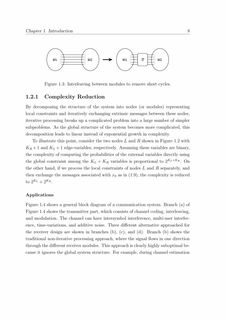
In most practical systems, modules are usually connected each other by bundles

of edges, and within each module there is usually a high correlation between adjacent

edge-variables. This setup will likely create many short cycles in the graph of the

system. Fortunately, it was found in practice that iterative algorithms usually con-

verge to solutions very close to optimal if the graph of the system has no short cycles.

For that reason, techniques like random interleaving between modules, as shown in

Figure 1.3, are commonly used to remove short cycles.

1.2 Benefits of Iterative Processing

In this section, we consider the practical benefits of iterative processing, and its

applications in communication systems.


�! #" �! #"$

Figure 1.3: Interleaving between modules to remove short cycles.

1.2.1 Complexity Reduction

By decomposing the structure of the system into nodes (or modules) representing

local constraints and iteratively exchanging extrinsic messages between these nodes,

iterative processing breaks up a complicated problem into a large number of simpler

subproblems. As the global structure of the system becomes more complicated, this

decomposition leads to linear instead of exponential growth in complexity.

To illustrate this point, consider the two nodes L and R shown in Figure 1.2 with

KR + 1 and KL + 1 edge-variables, respectively. Assuming these variables are binary,

the complexity of computing the probabilities of the external variables directly using

the global constraint among the KL + KR variables is proportional to 2KL+KR . On

the other hand, if we process the local constraints of nodes L and R separately, and

then exchange the messages associated with x0 as in (1.9), the complexity is reduced

to 2KL + 2KR .

Applications

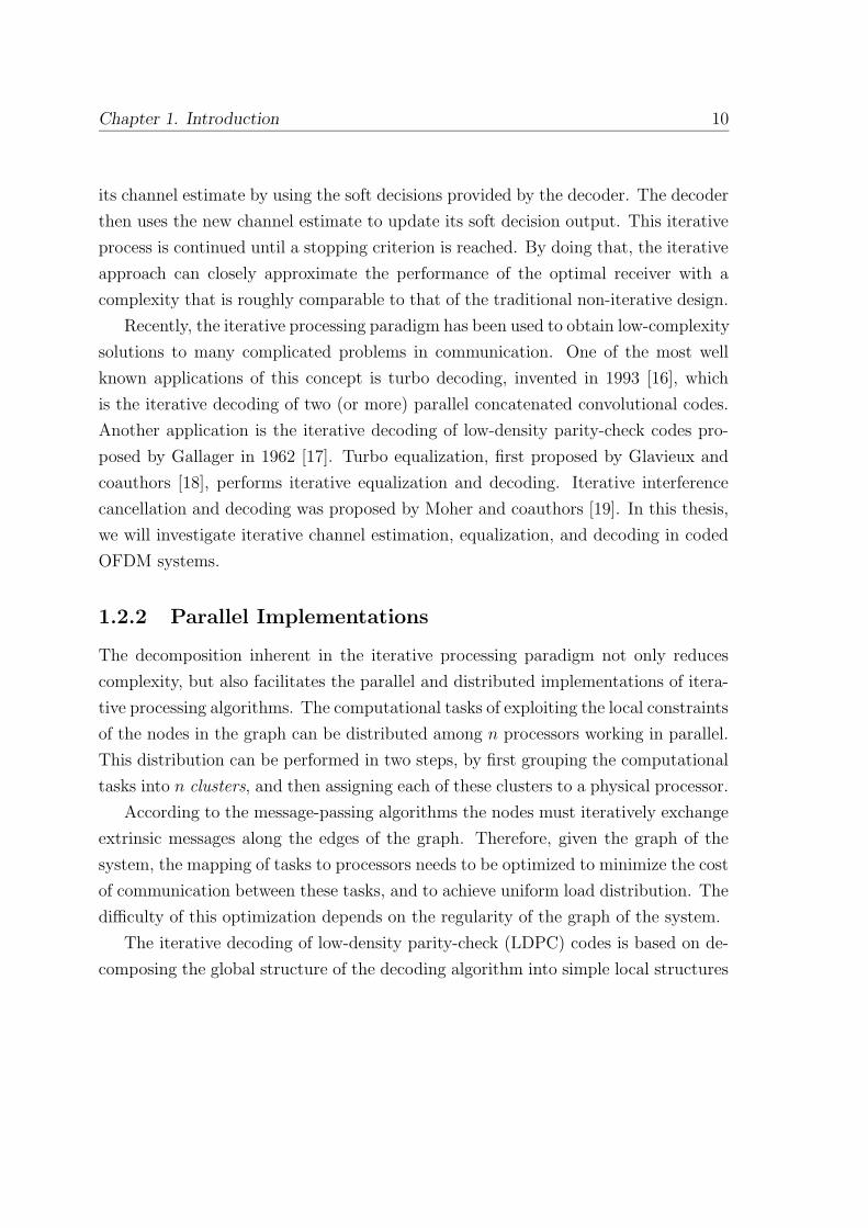
Figure 1.4 shows a general block diagram of a communication system. Branch (a) of

Figure 1.4 shows the transmitter part, which consists of channel coding, interleaving,

and modulation. The channel can have intersymbol interference, multi-user interfer-

ence, time-variations, and additive noise. Three different alternative approached for

the receiver design are shown in branches (b), (c), and (d). Branch (b) shows the

traditional non-iterative processing approach, where the signal flows in one direction

through the different receiver modules. This approach is clearly highly suboptimal be-

cause it ignores the global system structure. For example, during channel estimation


and channel mitigation, which may include equalization and interference cancella-

tion, the coding structure is ignored. Despite its highly sub-optimal performance,

this design is ubiquitous in practice because of its simplicity. Branch (c) shows the

optimal joint maximum-likelihood (ML) receiver, which attempts to find the most

likely transmitted sequence of information symbols given received signal. For most

non-trivial systems this approach is prohibitively complex to implement in practice.

%

&('*),+.-,/1032 45&/6&,+57 89): 2 ;3& : 2 )=<*<*>? 8,@BA 2 0C>�&=852 /32 <ED=/

FG<*>H- : +=0I2 <ED2 D=01&97 JK&97 &9D=8=&>L2 /106<*7 0I2 <EDD=<L2 /6& 89)5+.D�D,& :

>�&9FM<*>E- : +N032 <LD

>�&9FM<*>E- : +N032 <LD

>�&9FM<*>E- : +N032 <LD

? +9@ 89)5+.D�D,& :A 2 06/CJ17 <EF/O<E-�7 8N&P8N<*>�&97 8N<*>L2 D,Q

89),+.D�D,& :89),+.D�D,& :FR2 032 Q�+=032 <LD&N/60I2 FM+=0I2 <ED

89),+.D�D,& :89),+.D�D,& :&N/60I2 FM+=0I2 <EDFR2 032 Q�+=032 <LD

+=8=89-�7S+=01&P8�),+.D�D,& : FM<*>�& :

? A @ A 2 0C>�&=852 /32 <ED=/>.&N8N<*>�&97

? >L@ A 2 0C>�&=852 /32 <ED=/>.&N8N<*>�&97 %

%UTEV

%UTEV

Figure 1.4: Block diagram of a communication system.

Branch (d) shows a receiver design based on the iterative processing approach. In

this case, although each module processes the data according to its local structure,

as in the non-iterative approach in branch (b), the global structure of the system is

indirectly exploited by iteratively updating and exchanging extrinsic information be-

tween these modules. For example, the decision-directed channel estimator improves


its channel estimate by using the soft decisions provided by the decoder. The decoder

then uses the new channel estimate to update its soft decision output. This iterative

process is continued until a stopping criterion is reached. By doing that, the iterative

approach can closely approximate the performance of the optimal receiver with a

complexity that is roughly comparable to that of the traditional non-iterative design.

Recently, the iterative processing paradigm has been used to obtain low-complexity

solutions to many complicated problems in communication. One of the most well

known applications of this concept is turbo decoding, invented in 1993 [16], which

is the iterative decoding of two (or more) parallel concatenated convolutional codes.

Another application is the iterative decoding of low-density parity-check codes pro-

posed by Gallager in 1962 [17]. Turbo equalization, first proposed by Glavieux and

coauthors [18], performs iterative equalization and decoding. Iterative interference

cancellation and decoding was proposed by Moher and coauthors [19]. In this thesis,

we will investigate iterative channel estimation, equalization, and decoding in coded

OFDM systems.

1.2.2 Parallel Implementations

The decomposition inherent in the iterative processing paradigm not only reduces

complexity, but also facilitates the parallel and distributed implementations of itera-

tive processing algorithms. The computational tasks of exploiting the local constraints

of the nodes in the graph can be distributed among n processors working in parallel.

This distribution can be performed in two steps, by first grouping the computational

tasks into n clusters, and then assigning each of these clusters to a physical processor.

According to the message-passing algorithms the nodes must iteratively exchange

extrinsic messages along the edges of the graph. Therefore, given the graph of the

system, the mapping of tasks to processors needs to be optimized to minimize the cost

of communication between these tasks, and to achieve uniform load distribution. The

difficulty of this optimization depends on the regularity of the graph of the system.

The iterative decoding of low-density parity-check (LDPC) codes is based on de-

composing the global structure of the decoding algorithm into simple local structures


called bit nodes and check nodes that need to communicate with each other. In this

thesis, we will apply the above ideas to optimize the implementation of the iterative

LDPC decoding on programmable parallel architectures.

1.3 Overview

The common theme of this thesis is utilizing the idea of decomposing a global system

structure into simpler modules that iteratively exchange soft information for two pur-

poses. The first one is achieving close to optimal solutions to complicated problems.

The second one is using it as a first step towards parallel and distributed implemen-

tations of such systems. In particular, we will use this idea to perform joint channel

estimation and decoding in coded OFDM systems. Then, we will present architec-

tures and methodologies for code-independent parallel implementations of iterative

LDPC decoding.

Chapter 2 starts by presenting basic background information on modeling wireless

channels. It then introduces OFDM systems and explains the importance of coding

and interleaving in such systems to exploit frequency diversity. Chapter ?? explains

how the concept of iterative processing can be applied to exploit this already exist-

ing coding information in the channel estimation process. We present an iterative

channel estimation/equalization and decoding algorithm that exploits the global sys-

tem structure and leverage all the information that can be available to the receiver.

This algorithm can be used to blindly estimate the channel, or to track the channel

time variation on time-correlated channels. We also show how serial concatenation

with an outer LDPC code can be used to eliminate the error flooring effect caused

by the occasional misconvergence of the iterative algorithm. LDPC codes and their

iterative decoding are introduced in Chapter ??, which also presents the motivations

for parallel and programmable decoding of these codes. Methodologies for parallel

implementations of iterative LDPC decoding on programmable parallel machines are

then presented in Chapters ?? and ??. Chapter ?? concludes the thesis and suggests

directions for future work.

The original research contributions of this thesis include the following:


• An iterative algorithm for blindly or semi-blindly estimating the channel in

coded OFDM systems (Chapter ??) [20, 21].

• An iterative algorithm for tracking the channel time variation in coded OFDM

systems (Chapter ??) [22].

• Showing that, for the purpose of iterative channel estimation and decoding, the

Max-Log-MAP algorithm is the most attractive algorithm from both implemen-

tation and performance prospectives for SISO decoding of convolutional codes

in coded OFDM systems (Chapter ??) [20].

• Proposing the use of serial concatenation with an outer LDPC code to offer a

trade-off between latency and performance without increasing the complexity of

the iterative channel-estimation-and-decoding process, which uses only a simple

4-state convolutional code (Chapter ??) [22].

• A new low-complexity shared-memory parallel architecture and the associated

memory management scheme for programmable LDPC decoding (Chapter ??) [23,

24].

• Low-complexity algorithms for optimizing the mapping and scheduling of de-

coding tasks to processors of the proposed parallel architecture so as to decrease

the decoding latency and increase throughput (Chapter ??) [23, 24].

• Low-complexity algorithms for optimizing the mapping of decoding tasks to

processors of general-purposed message-passing parallel architectures so as to

minimize the communication cost (Chapter ??) [25, 26].

1.4 Notation

In the rest of this thesis, the following conventions hold:

• p(·) is used to denote a probability density, while P (·) is used to denote a real

probability.


• LLR(x) denotes the log-likelihood ratio of a binary variable x.

•∑

∼x0

indicates that the sum is over all variables except x0.

• µL→R(x0) is the soft message associated with the edge-variable x0 passed from

node L to node R.

• Vectors are denoted by lower-case bold letters.

• Matrices and frequency-domain vectors are denoted by upper-case bold letters.

• AT is the transpose of matrix A.

• A∗ is the conjugate-transpose of matrix A. When ∗ is used with a scalar, it

denotes a complex-conjugate.

• E(x) is the expectation of the random vector x.

• E(A) is the expectation of the random matrix A.

• Cov[A] is the covariance matrix of A.

• Ik is the k × k identity matrix.

• 0k×n is the k × n matrix with all elements being 0.

• diag(a1, . . . , aK) is the diagonal matrix formed by a1,. . . ,aK .

• ⊗ denotes a cyclic convolution.

• � denotes a point-wise product.

• Re(x) is the real part of x.

• Im(x) is the imaginary part of x.

• x is the time average of x.

• bxc is the largest integer smaller than or equal to x.


• S \ x denotes the set S with the element x excluded.

• |S| is the number of elements in the set S.

• deg(b) is the degree of node b.

• Nbr(b) is the set of neighbors of node b, where |Nbr(b)| = deg(b).

Chapter 2

Coded Orthogonal Frequency

Division Multiplexing

Dispersiveness and non-stationarity are the main difficulties associated

with wireless channels. Dispersiveness is caused by their multi-path nature,

which causes intersymbol interference (ISI). Orthogonal frequency-division multiplex-

ing (OFDM) combined with appropriate coding and interleaving is an effective tech-

nique for mitigating ISI on these channels. Coherent detection enables the use of ef-

ficient multi-amplitude modulations, but requires channel estimation at the receiver.

In coded OFDM systems, exploiting the coding information in estimating the channel

can result in significant performance improvement.

This Chapter provides some background information on coded OFDM systems in

preparation for Chapter ??. Section 2.1 gives a brief overview on wireless channels and

how they can be modeled. Multicarrier modulation techniques are then introduced in

Section 2.2. Section 2.3 reviews the fundamentals of error control coding and explains

the importance of proper coding and interleaving for wireless OFDM systems. Various

channel estimation techniques for OFDM systems are briefly reviewed in Section 2.4,

which also motivates taking advantage of the code during this process.

15

Chapter 2. Coded Orthogonal Frequency Division Multiplexing 16

2.1 Wireless Channel Model

When transmitting a signal in a wireless environment, the signal is affected by the

geometry of the environment, the movement of the receiver or the environment, and

the carrier frequency of the signal. The more scatterers in the environment, the more

signals that arrive at the receiver. These signals arrive at different times depending

on how far the scatterers are from the receiver.

This communication channel is known as a multi-path channel [27]. At a fixed

moment of time, the channel impulse response can be characterized by

h(τ) =L−1∑

k=0

αkδ(τ − τk), (2.1)

where L is the number of resolvable paths that arrive at the receiver, which depends on

the bandwidth and the sampling rate at the receiver. The parameters αk and τk rep-

resent the attenuation and delay of the kth path, respectively. The root-mean-square

value of the delay, τrms, is called the delay spread of the channel, and τL−1 is called

the maximum delay spread. Assuming that the transmitted signal x(t) modulates a

carrier frequency fc, the received signal is then

y(t) =L−1∑

k=0

αkx(t − τk)ej2πfc(t−τk) + n(t), (2.2)

where n(t) is an additive white Gaussian noise (AWGN).

Multiple paths can arrive simultaneously at the receiver and will combine con-

structively or destructively depending on the relative phases of their waves. Using a

central limit theorem argument [7], αk is a complex Gaussian random variable [27].

When L > 1, the channel is said to be dispersive, and it exhibits frequency selectiv-

ity. This dispersiveness causes intersymbol interference (ISI), where the main cause

of distortion can be the system’s own data.


2.1.1 Modeling Channel Time-Variation

In a wireless channel, the environment can change because of the movement of the

receive, or the environment itself. These changes fall into two categories: short-term

fading and long-term fading. Short-term fading is manifested as a Doppler spread

in the frequency domain, which is determined as the width of the spectrum when

a single sinusoid is transmitted [28]. The maximum Doppler frequency is fD = vfc

c,

where v is the relative speed of the receiver, c is speed of light, and fc is the carrier

frequency. The channel time correlation function and the Doppler power spectrum

are related through a Fourier transform [29]. Long-term fading or shadowing is due to

gross changes in the environment, and is caused by mountains, buildings, and other

large obstacles blocking the signal.

The absolute value of αk has a Rayleigh distribution if there is no direct path

(line-of-sight) from the transmitter to the receiver, and a Rician distribution if there

is a direct path [27]. The Rayleigh distribution has the form

pR(rk) =rk

Γk

exp

(

−r2k

2Γk

)

, (2.3)

where rk = |αk|, and Γk = E [|αk(t)|2]. The Rician distribution has the form

pR(rk) =rk

Γk

exp

(

−r2k + r2

k,0

2Γk

)

I0

(

−rkrk,0

2Γk

)

, (2.4)

where I0 is a modified zeroth order Bessel function, and rk,0 is the mean amplitude

of the line-of-sight component of the kth path. In the Rayleigh fading case, we are

often interested in the distribution of the signal power, γk = |αk|2, which is given by

p(γk) =1

2Γk

exp

(

−γk

2Γk

)

. (2.5)

Due to the long-term fading, the variance Γk is itself a random variable that has a

log-normal distribution [27]. This log-normal variation occurs on a scale of tens to

hundreds of feet, while the Rayleigh fading occurs on a scale of the wavelength of the


signal.

The power-delay profile of the channel is defined as [27]

p(τ) = E[h(t, τ)h∗(t, τ)], (2.6)

where h(t, τ) =∑L−1

k=0 αk(t)δ(τ − τk). Assuming that αi(t) is uncorrelated with αj(t)

for i 6= j, which simplifies the analysis, and has been shown to be true in most

measurements [30, 31], we obtain

p(τ) =L−1∑

k=0

E[

|αk(t)|2]

δ(τ − τk), (2.7)

=L−1∑

k=0

Γkδ(τ − τk). (2.8)

In indoor radio environments, it was found that the channel power profile is an ex-

ponentially decaying function of the excess delay, τ , and the amplitudes of individual

multipath components are Rayleigh distributed [32, 33].

A commonly used model for the time variation of the channel is the Jakes’ spec-

trum [27], where the time correlation of the channel taps is given by

ρ(δt) = J0(2πfDδt), (2.9)

where J0 is a zeroth order Bessel function, and fD is the maximum Doppler frequency.

The coherence time defined as Tc = 12πfD

is the time duration over which the

channel characteristics do not change significantly [29]. Clearly, if fD is larger, the

channel response will change more rapidly in time. Similarly, the coherence bandwidth

defined as Bc = 12πτrms

, where τrms is the delay spread of the channel, is the frequency

band over which the channel frequency response is almost constant [29]. As the

channel delay spread increases, the channel’s frequency selectivity increases, leading

to more sever ISI.


2.1.2 Diversity

On frequency- or time-selective channels, error control coding by itself is not enough

to achieve low probability of error. One way to further lower the probability of

error is through diversity [27]1. The concept behind diversity is based on the fact

that the probability that two independent channels have low SNRs is smaller than

the probability that either one of the channels has a low SNR. Diversity attempts

to transmit the same information on multiple (hopefully independent) channels to

decrease the average probability of error on fading channels.

There are three basic types of diversity used in wireless systems: time diversity,

frequency diversity, and spacial diversity. In time diversity, the information is repli-

cated and spread over time in such a way that the information appears on independent

channels. Thus, for slowly time-varying channels (with relatively large coherence time

Tc), the information needs to be spread over a long period of time, which may not

be possible for latency-sensitive applications. In frequency diversity, the information

is spread across two or more independent frequency carriers. Frequency diversity is

specially attractive in wideband systems, where the channel is frequency selective

(coherence bandwidth Bc � B, where B is the bandwidth of the channel). In spa-

cial diversity, the receiver uses two or more antennas spaced half a wavelength (λ/2)

apart to ensure independent channels [27]. The required antenna spacing can even

be much larger than λ/2 in environments with low angle-spread. If the receiver is

moving, it can receive the signals arriving at different points in space at different

times. Therefore, time and spatial diversity are two sides of the same coin in that

case.

There are variations of diversity combining depending on the weighting given

to the signal received on each of the independent channels carrying the redundant

information. For example, selection diversity simply selects the largest of the received

signals. On the other hand, in maximam-ratio diversity combining, the component

channels are weighted by their respective channel SNRs. Selection diversity typically

has a 2 dB loss relative to maximum-ratio diversity combining [29, 27].

1It is worth mentioning that if the code is designed properly it can simultaneously exploit diversity

in addition to offering a coding gain.


2.2 Multicarrier Modulation

Multicarrier modulation (MCM) has long been considered a candidate for modulation

on channels with sever intersymbol interference (ISI). An early use of MCM is the

1958 Kineplex modem [34] designed by the Collins Radio Company. Research in

MCM techniques can be traced back to Holsinger [35], and later to Chang [36] and

Saltzberg [37]. Multicarrier transmission systems attempt to subdivided the total

bandwidth of the ISI channel into a bank of orthogonal narrow-band subchannels.

Data are then transmitted in parallel over these subchannels, thereby avoiding high-

speed equalization and alleviating impulsive noise.

Consider an additive white Gaussian noise (AWGN) channel with frequency re-

sponse H(f) as shown in Figure 2.1, and noise variance σ2. The channel can be

partitioned into N subchannels, each with a carrier frequency fn. If N is large, the

bandwidth of each subchannel will be so small that the frequency response over it

can be approximated as constant. This flat response corresponds to ISI-free trans-

mission. Thus, each subchannel can be modeled as a flat AWGN channel with a

scalar gain H(fn) and noise variance σ2. Since the subchannels are orthogonal, each

subchannel is modulated separately, with modulation and demodulation performed

in the frequency domain.

2.2.1 DFT-Based Channel Partitioning

In 1971, Weinstein and Elbert [38] applied the discrete Fourier transform (DFT) to

multicarrier transmission systems as part of the modulation and demodulation pro-

cesses. The DFT-based approach eliminated the need for the banks of subcarrier

oscillators and coherent demodulators required by earlier frequency-division multi-

plexing techniques. It enabled a completely digital implementation that can take

advantage of recent advances in high-speed digital signal processing (DSP) and very

large scale integrated circuits (VLSI) technologies. In practical systems, fast Fourier

transform (FFT) algorithms [39], which reduce the complexity of an N -point DFT

operation from O(N 2) to O(N log N), are typically used as computationally efficient

means of domain conversion.


WYX[Z.\^]�W

\\�_a`�b

WYX[Z.\�c�]�W

\�c\Cd

Figure 2.1: Channel partitioning in multicarrier modulation.

The use of FFT/IFFT for domain conversion selects the set {e−j2πfnt} as the

basis functions for transmission, where fn = nNT

, where T is the symbol period, N

is the number of subchannels, and n = 0, 1, . . . , N − 1. The set {e−j2πfnt} is also

a set of eigenfunctions of any circulant matrix. Therefore, by making the channel

impulse response matrix circulant, we achieve two additional advantages to using the

set {e−j2πfnt} as basis functions in addition to the low implementation complexity.

First, the subchannels that result from this set of basis functions are orthogonal; thus,

each can be modulated and demodulated separately. Second, these basis functions

are independent of the channel response, so the same modulator and demodulator

can be used on a variety of channels.

The impulse response of a transmission channel can be modeled as a circulant

matrix with a simple trick known as the cyclic-prefix [40]. The vector of N sampled

output of an AWGN channel with L(= ν + 1)-tap impulse response {h0, h1, . . . , hν}


can be written as

yN−1

yN−2

...

y1

y0

=

h0 h1 . . . hν 0 0 . . . 0

0 h0 h1 . . . hν 0 . . . 0...

. . . . . . . . . . . . . . . . . ....

0 . . . 0 h0 h1 . . . hν 0

0 . . . 0 0 h0 h1 . . . hν

xN−1

xN−2

...

x1

x0

xpN−1...

xpN−ν

+

nN−1

nN−2

...

n1

n0

(2.10)

y = PxN+ν + n (2.11)

where x =[

xN−1 xN−2 . . . x1 x0

]T

is the block of N channel input samples,

(xpN−1, . . . , x

pN−ν) are the last ν samples of the previous input block, and n is an

AWGN noise vector. For the purpose of computing y, the channel input can be made

to appear periodic by inserting the cyclic-prefix x =[

xN−1 xN−2 . . . xN−ν

]T

between x0 and xpN−1. The addition of this length ν cyclic-prefix causes a slight loss

of NN+ν

in information rate. However, the channel output can now be expresses as

yN−1

yN−2

...

y1

y0

=

h0 h1 . . . hν 0 . . . 0

0 h0 h1 . . . hν. . . 0

0. . . . . . . . . . . . . . . 0

0 . . . 0 h0 h1 . . . hν

hν 0 . . . 0 h0 . . . hν

.... . . . . . . . . . . . . . .

...

h1 . . . hν . . . 0 . . . h0

xN−1

xN−2

...

x1

x0

+

nN−1

nN−2

...

n1

n0

(2.12)

y = P x + n (2.13)

where the channel impulse response matrix P is now circulant as desired.

Another advantage of the cyclic-prefix is that it provides a guard interval that


prevents intersymbol interference caused by the multipath channel. This fact is evi-

dent in (2.12), where the output block y is dependent only on the current input block

x through a cyclic convolution. Note that to completely eliminate ISI and maintain

orthogonality among the subchannels, the cyclic-prefix extension has to be at least

as long as the maximum delay spread of the channel. The output of the channel in

the frequency domain can then be obtained as

Y = diag(H)X + N , (2.14)

where X = Qx,Y = Qy,N = Qn, and H = V h, where Q is an N × N DFT

matrix, and V is an N×L Vandermonde matrix with elements given by Vn,l = e−j 2π

Nnl

for n = 0, 1, . . . , N − 1 and l = 0, 1, . . . , L − 1.

Figure 2.2 shows a typical FFT-based MCM system. The incoming serial data

is first converted from serial to parallel and grouped into bn bits. Each group of

bits selects a constellation point Xn for subchannel n, where n = 0, 1, . . . , N − 1.

The block of N complex numbers is then modulated by the inverse FFT (IFFT) and

converted to time-domain serial data for transmission. The cyclic-prefix is added,

and the signal is transmitted across the ISI channel. At the front end of the receiver,

the cyclic-prefix is removed, the signal is converted back to parallel, and then to the

frequency domain via the FFT. The signal of each subchannel is then independently

equalized using a single-tap frequency equalizer with gain 1Hn

, and then passed to an

AWGN slicer to yield the detected symbol Xn.

2.2.2 DMT and OFDM

The DFT-based MCM is usually called discrete multitone (DMT) modulation. On

slowly time-varying two-way channels, such as telephone lines, DMT optimizes the

spectrum of the transmitted signal, Sx(f), across the subchannels using what is called

“water-filling” [41]. As shown in Figure 2.3, this optimization is performed by allo-

cating energy, or equivalently bits, to subchannels in proportion to their SNRs. In the

1990’s, DMT technology has been exploited in many applications, particularly, those


e�f.fg(h5g9i j gk5lYm(n*oprq*s tttttt

ttt

tttttt

tttttt

p m5l j u.i f u,v6uj w k.x v

y�z u�w.w m i

{ |H|.} sUq9pp j ~Lw9u.i� u k.k.m5l

�O�� j v6� ��

��r�

gNh5g5i j gk9lSm(n*o� m5��9�5mpHq*sm=�Ex u.i j � m5l �

�� w m(� v6u kp j ~Lw�u�if m9� u k.k�m9lsUq�p

��

�� r�|H|.}p m9l j u�i f u=vOu�Lx v k.x v

Figure 2.2: A DFT-based MCM system.

for offering broadband access over twisted pairs. Such applications include high-bit-

rate digital subscriber lines (HDSL) [42], asymmetric digital subscriber lines (ADSL),

and very high-speed digital subscriber lines (VDSL) [43, 44].

The water-filling optimization not only exploits the frequency diversity of the

ISI channel, but is also the capacity achieving approach [41]. However, it requires

knowledge of the channel at the transmitter [45]. On broadcast channels or fast time-

varying channels, like mobile wireless channels, timely feedback to the transmitter

can be very difficult or impossible. In such cases, where the transmitter has no

knowledge of the channel, equal energy and equal number of bits are assigned to each

subchannel, as shown in Figure 2.4. When there is no water-filling optimization in a

multitone system, it is often referred to as orthogonal frequency-division multiplexing

(OFDM). Given a long enough period of time, each subchannel is subject to the same

fading statistics, and has the same average SNR. In this case, assigning an equal

number of bits to each subchannel can be shown to be appropriate via a minimax

argument - minimizing the maximum bit error rate over a set of possible SNRs on

each subchannel [46, 47].


�

�^��*�� I�� 9�

Figure 2.3: Water-filling optimization in DMT systems.

In a frequency-selective channel, where different subchannels have different gains,

the bit error rate (BER) of the OFDM system will be largely determined by the

few subchannels with the smallest gains. To avoid this domination by the weakest

subchannels, forward-error correction (FEC) coding across subchannels and inter-

leaving are used to exploit frequency diversity. This technique is what is referred

to as coded OFDM (COFDM). The topic of coding and how it provides diversity in

an OFDM system will be discussed in the next Section. Another way to exploit fre-

quency diversity is to spread each information symbol across multiple subchannels, as

in multicarrier code-division multiple-access (MC-CDMA) [48, 49] and block-spread

multicarrier [50]. However, unlike coded OFDM, these alternatives do not offer any

coding gain. Since the coding gain is essential for proper system operation in a

wireless fading environments, most practical wireless systems use coded OFDM or

combine coding with one of the above spreading techniques.

OFDM has been particularly successful in numerous wireless applications, where

its superior performance in multi-path environment is desirable. It has been adopted

in digital audio/video broadcasting (DAB/DVB) standards in Europe [51, 52]. A


¡�¢¤£R¥

¦K§©¨*ª¬«#¦

¯® ¨*ª¬«

ª

Figure 2.4: Transmit spectrum of an OFDM system.

particularly interesting configuration enabled by OFDM technology is the single-

frequency broadcast (SFN) network [53, 1], where many geographically separated

transmitters broadcast identical and synchronized audio or video signals to offer a

better coverage of a large region. The reception of such signals by the receiver

is equivalent to an extreme form of multi-path. Another wireless application of

OFDM is in high-speed local area networks (LANs) [54]. OFDM technology has

already been adopted in multiple broadband mobile wireless LAN standards, such as

IEEE802.11a [2], MMAC, and HIPERLAN/2 [3].

2.3 Coding Fundamentals

To transmit data at rates close to the capacity, it is necessary to introduce schemes

to correct for the noise and distortion introduced by the channel. In error-control

coding, controlled redundancy is introduced in the transmitted data for the purpose

of correcting or detecting errors. The basic principle behind error-correcting codes

is to increase the separation between possible transmitted sequences of symbols in a


bandwidth-efficient manner. In a stationary channel, increasing the Euclidean dis-

tance between sequences of symbols is sufficient to reduce the probability of error.

However, that is not enough in a fading channel. We must also increase the diversity

factor of the received signal. To do this, coding must use interleaving and be designed

specifically to exploit diversity.

OFDM is an effective technique for mitigating ISI and is typically used on wide-

band frequency-selective channels. Using the proper coding and interleaving across

subchannels is essential to exploit frequency diversity on such channels. If latency

can be afforded, coding and interleaving across OFDM symbols can further be used

to exploit time diversity or to combat bursty errors.

The simplest way to correct errors in a transmission would be to retransmit the

same symbol multiple times, and use a majority decoder at the receiver. This ap-

proach, however, is not bandwidth efficient. There are two types of codes developed

for static AWGN channels: block codes and convolutional codes (including trellis-

coded modulation). They are briefly introduced in the subsections below, along with

how they can be made appropriate for fading channels.

A rate- kn

code takes k input information bits and outputs n coded bits. In the

systematic form of the code, the input bits are transmitted as part of the output

sequence. In searching for the most likely transmitted sequence, the decoder can

use either sliced bit values (0 or 1), or the received noisy symbol values. If it uses

the sliced bits, the process is called hard-decoding, because the receiver makes ‘hard’

decisions before passing the coded data to the decoder. On the other hand, in soft-

decoding, the decoder uses the noisy received symbols. In a hard-decoding system,

some information (the actual size of error in the analog domain) is lost by the receiver.

Thus, in general, a hard decoder performs worse than a soft decoder. A soft-input

soft-output (SISO) decoder not only uses soft input information, but also produces

soft output information to be used by other modules at the receiver. This feature is

essential to the iterative processing paradigm; thus, in this thesis, we will limit our

attention to SISO decoders.


2.3.1 Block Codes

In a rate- kn

block code, input data are blocked into k symbols, and each block is

mapped into an output block of n symbols called a codeword, where n > k. Only M k

of the possible Mn output blocks are legitimate codewords, where M is the number of

symbols levels. The Hamming distance between codewords is the number of symbols

where the codewords differ. A figure of merit of a block code is its minimum distance,

dmin ≤ n − k + 1 [55], which is the smallest Hamming distance between any two

codewords. At the receiver, the decoder finds the codeword that is closest in some

sense2 to the received block of n symbols corrupted with noise. In hard decoding, for

example, a block code with a minimum distance dmin can detect up to dmin −1 errors

or correct up to b 12(dmin − 1)c errors [56].

A class of binary block codes that has excellent error-correction capabilities and

low-complexity SISO decoding is the class of low-density parity-check codes [17].

Chapter ?? presents more details about these codes and their iterative soft decoding.

2.3.2 Convolutional Codes

Convolutional codes are bit-oriented codes that take a sequence of input symbols

u(D), convolve them over the field GF (2) with the generator matrix of the code

G(D), and output the sequence of coded symbols cT (D) = u(D)G(D). By introduc-

ing memory in the output symbols, the encoder restricts the possible set of legitimate

sequences. For example, consider the rate-1/2 convolutional encoder with the gen-

erator matrix G(D) =[

1 + D + D2 1 + D2]

. The recursive systematic form of

this encoder is given by G(D) =[

1 1+D2

1+D+D2

]

and is shown in Figure 2.5. This

code is a 4-state code, where the state is represented by the information bits s0 and

s1, stored in the delay elements D and D2. The memory or constraint length of this

code is m = 2. The trellis diagram, which is a state diagram with an additional time

dimension, of the 4-state recursive systematic convolutional (RSC) code is shown in

Figure 2.6. The encoder will only output sequences of symbols that match the trellis

of the code.

2Hamming distance for hard decoding, or Euclidean distance for soft decoding.


It is possible for the input and output of the convolutional encoder to be continu-

ous streams. However, to improve the decoding performance and reduce the system

latency, it is more common to periodically terminate and restart the code. Over a

coding interval, the encoder starts at a given state and is forced to terminate at a

given (usually the same) state. This condition enables the decoder to optimally and

independently decode the symbols over this interval. The coding interval could, for

example, correspond to a single OFDM symbol.

°*± °E²³ ³

´�µ ¶5µ5·¶5µ=¸

Figure 2.5: A rate-1/2 4-state recursive systematic convolutional(RSC) encoder.

Trellis (or sequence) decoding of convolutional codes is based on finding the path

through the trellis that is closest in some sense3 to the received sequence. The Viterbi

algorithm (VA) [57] is an efficient dynamic programming algorithm for maximum-

likelihood sequence decoding (MLSD) of convolutional codes. The VA algorithm,

however, does not output soft information. A modified version that generates soft-

output information is called soft-output Viterbi algorithm (SOVA) [58], but its soft

output is suboptimal. The maximum a posteriori (MAP) decoding algorithm [59] and

its derivatives the Log-MAP and Max-Log-MAP decoding algorithms [60] produce

optimal soft-output information for MAP symbol or sequence detection. More details

on the optimal SISO decoding algorithms for convolutional codes are presented in

3Hamming distance for hard decoding, or Euclidean distance for soft decoding.


¹Rº

º�¹

¹#¹

º#º

»9¼C½U¾¿¼�À¿ÁÂ�ÃÅÄÇÆÂ�ÃÅÄÉÈ

¹#¹º#º

¹Rº

º�¹

º#º ¹#¹

¹Rºº�¹

»5Ê ÃEË ¾�Ê Ã¿Ì Á

Figure 2.6: The trellis diagram of the 4-state RSC encoder.

Chapter ??.

2.3.3 Trellis Codes

A trellis code uses a rate-k/n convolutional encoder, but does not require a bandwidth

expansion [61]. Instead, the constellation size is expanded by a factor of 2n−k. The

constellation is then partitioned into 2n cosets with large Euclidean distance between

points within each coset. For example, Figure 2.7 shows a 16-QAM constellation that

is partitioned into 4 cosets labeled 0, 1, 2, and 3. Given b input information bits, k

bits of them are encoded by the convolutional encoder producing n coded bits that are

then used to select one of the 2n cosets. The remaining b − k bits are not coded and

are used to select one of the 2b−k points within the selected coset. The constellation

points in a coset represent parallel branches in the trellis of the code. The trellis code

increases the minimum Euclidean distance in two ways: between points within a coset

(or parallel branches) through partitioning, and between cosets through convolutional


coding. The smaller of these two distances determines the performance of the code.

ÍÍÎÎ ÏÏÐÐ

ÑÑÒÒÓÓÔÔ

Õ Õ

Õ Õ

Ö Ö

Ö Ö

×

×

×

×

Ø

Ø Ø

Ø

Ù

Ú

Figure 2.7: A 16-QAM constellation partitioned into 4 cosets.

Although the above trellis coding approach provides a large minimum Euclidean

distance, which is enough for an AWGN channel, the minimum Hamming distance is

only 1, because bits within a coset are left uncoded. Hence, if one trellis-coded symbol

is lost, this immediately results in one of more bit errors. Such codes perform poorly in

time- or frequency-selective fading channels, because they fail to exploit diversity. To

exploit diversity, an additional requirement to the large minimum Euclidean distance

is that the Euclidean distance be spread over as many symbols as possible [62], i.e.,

the code should also have a large minimum Hamming distance. For this reason,


OFDM systems do not typically use conventional multilevel trellis coding, which has

uncoded bits. Instead, they use what is called pragmatic coding, where all information

bits are encoded by a convolutional encoder, and then the coded bits are mapped to

constellation points according to a specific mapping function [1].

2.3.4 Interleaving

In general, transmission errors have a strong time/frequency correlation. Interleaving

randomizes the data so that errors in the data appear to be independently distributed.

Interleaving can be combined with coding to add diversity to the received signal, which

is a key to reducing error probability for a coded system in a time- or frequency-

selective channel. Bursty errors due to time- or frequency-correlated fading can cause

the code to fail. Interleaving distributes these errors more evenly, and potentially

over multiple codewords, giving the code a better chance of correcting the errors.

Interleaver depth should be large enough (relative to the coherence time or coherence

bandwidth of the channel) to break long burst of errors. There are many types of

interleavers including: block, convolutional, and random interleavers [63].

2.4 Channel Estimation

As long as the cyclic-prefix extension is longer than or equal to the channel maximum

delay spread, equalization in multicarrier systems is very simple . The N subchannels

can be equalized independently in the frequency domain using N single-tap equalizers

with 1Hn

tap coefficient for each. Maximum-likelihood (ML) decisions can then be

made by passing the output of the equalizer through an AWGN slicer. This approach

is called coherent detection and requires estimating the subchannel complex gains Hn,

for n = 0, 1, . . . , N − 1, at the receiver. Channel estimation at the receiver can be

avoided by using differential detection; however, that leads to about 3 dB loss in SNR

compared to coherent detection [29]. Differential detection also typically requires the

use of constant-amplitude modulation, like differential phase-shift keying (DPSK),

thereby restricting the number of bits per constellation point.


There are many techniques for estimating the channel in OFDM systems. If

the channel is changing slowly, it can be estimated periodically by sending known

OFDM pilot symbols. The channel estimates obtained using the pilot symbols are

used to detect the data OFDM symbols in between the pilot symbols. Between pi-

lot symbols, the slow channel changes can be tracked using decision-based tracking

techniques [64, 65, 66]. If the channel is changing rapidly, known pilot tones can be

transmitted in each OFDM symbol to estimate the channel. These pilot tones are

typically distributed over a two-dimensional grid with time and frequency spacings

determined by the coherence time and coherence bandwidth of the channel, respec-

tively. Estimates of the complex gains of remaining subchannels are then obtain by

interpolation [1].

To avoid bandwidth-consuming training sequences, blind channel estimation tech-

niques that require no pilots have also been suggested [67, 68, 69, 70]. However, most

of these techniques typically require averaging over a large number of OFDM symbols

to reach to a sufficiently accurate estimate of the channel. This requirement not only

increases the latency of the system, but also limits the use of these techniques to

slowly time-varying channels.

In channel estimation, there are multiple performance objectives. The first one is

to reduce the noise in the channel estimate by, for example, minimizing the estimate

mean-square error (MSE) defined as

MSE = ||h − h||2 (2.15)

where h is the channel impulse response in the time domain, and h is the channel

estimate. The second objective is to minimize of the training overhead by minimizing

the average number of pilots required to obtain a timely and sufficiently accurate es-

timate of the channel. Moreover, it is desirable to obtain a good estimate of the chan-

nel within as little number of OFDM symbols as possible, preferably, within a single

OFDM symbol. This requirement is particulary important in a packet transmission

system, such as an IEEE 802.11a wireless LAN, which requires an acknowledgment

to be sent after each packet transmission [2]. Any delay in the reception of a packet


will also delay the acknowledgement, and hence, decrease the effective throughput of

the system. To meet these objectives, in estimating the channel, the receiver must

exploit all the available system and data constraints, one of the most important which

is the coding information.

2.4.1 Exploiting the Code

As we have seen, the use of coding across subchannels is essential in wireless OFDM to

exploit frequency diversity on frequency-selective channels. Traditional coded OFDM

receivers typically ignore this coding information while estimating the channel by

separating the channel estimation process from the decoding process. Significant

performance improvements can, however, be achieved by properly combining these

two processes.

Let X be the transmitted OFDM data symbol, Y be the received OFDM symbol

including the cyclic prefix observation, and H be the channel response in the fre-

quency domain. Ideally, we would like to solve the following join ML channel and

data estimation problem:

(

X, H)

= arg maxX ,H

{

p(

Y |X, H)}

. (2.16)

However, the optimal solution to this problem is overly complex for practical imple-

mentations. Chapter ?? shows how the iterative processing paradigm can be used

to offer an attractive trade-off between performance and complexity in solving this

problem.

2.5 Remarks

This chapter provided a brief overview of wireless channels and how they can be

modeled. It also briefly introduced OFDM as an effective technique for mitigating

ISI on frequency-selective channels. Appropriate coding and interleaving are essential

to exploit frequency diversity on these channels. The receiver should attempt to take


advantage of this already existing coding information in estimating or tracking the

channel, which is required for coherent detection. Low-complexity iterative algorithms

for achieving this purpose will be presented in Chapter ??.

Bibliography

[1] R. van Nee and R. Prasad, OFDM for wireless multimedia communications.

Artech House, 2000.

[2] IEEE, “Supplement to standard for telecommunications and information ex-

change between systems—LAN/MAN specific requirements—part 11: Wireless

MAC and PHY specifications: High speed physical layer in the 5-GHz band,”

P802.11a/D7.0, July 1999.

[3] ETSI, “Broadband radio access networks (BRAN); HIPERLAN type 2 technical

specifications part 1—physical layer,” DTS/BRAN030003-1, Oct. 1999.

[4] V. Tarokh, N. Sechadri, and A. R.Calderbank, “Space-time codes for high data

rate wireless communication: Performance criterion and code construction,”

IEEE Trans. Inform. Theory, vol. 44, pp. 744–765, Mar. 1998.

[5] D. Agrawal, V. Tarokh, A. Naguib, and N. Seshadri, “Space-time coded OFDM

for high data-rate wireless communication over wideband channels,” in Proc.

IEEE Vehicular Tech. Conf., (Ottawa, Canada), pp. 2232–2236, May 1998.

[6] E. Biglieri, G. Caire, and G. Taricco, “Limiting performance of block-fading chan-

nels with multiple antennas,” IEEE Trans. Inform. Theory, vol. 47, pp. 1273–

1289, May 2001.

[7] A. Papoulis, Probability, Random Variables, and Stochastic Processes. McGraw-

Hill, 3rd ed., 1991.

36

BIBLIOGRAPHY 37

[8] J. G. D. Forney, “Codes on graphs: normal realizations,” IEEE Trans. Inform.

Theory, vol. 47, pp. 520–548, Feb. 2001.

[9] J. L. Fan, Constrained Coding and Soft Iterative Decoding. Kluwer Academic

Publishers, 2001.

[10] F. R. Kschischang, B. J. Frey, and H. A. Loeliger, “Factor graphs and the sum-

product algorithm,” IEEE Trans. Inform. Theory, vol. 47, pp. 498–519, Feb.

2001.

[11] S. M. Aji and R. J. McEliece, “The generalized distributive law,” IEEE Trans.

Inform. Theory, vol. 46, pp. 325–343, Mar. 2000.

[12] R. M. Tanner, “A recursive approach to low complexity codes,” IEEE Trans.

Inform. Theory, vol. 27, pp. 533–547, Sept. 1981.

[13] N. Wiberg, Codes and Decoding on General Graphs. PhD thesis, Linkoping

Studies in Science and Technology, Sweden, 1997.

[14] S. M. Aji, G. B. Horn, and R. J. McEliece, “On the convergence of iterative

decoding on graphs with a single cycle,” in Proc. CISS 98, (Princeton), Mar.

1998.

[15] Y. Weiss, “Correctness of local probability propagation in graphical models with

loops,” Neural Comput., vol. 12, pp. 1–42, 2000.

[16] C. Berrou, A. Glavieux, and P. Thitimajshima, “Near Shannon limit error-

correction coding and decoding: turbo-codes,” in Proc. IEEE Int. Conf. Com-

mun., (Geneva, Switzerland), pp. 1064–1070, May 1993.

[17] R. G. Gallager, “Low-density parity-check codes,” IRE Trans. Inform. Theory,

vol. IT-8, pp. 21–28, Jan. 1962.

[18] A. Picart, P. Didier, and A. Glavieux, “Turbo-detection: a new approach to com-

bat channel frequency selectivity,” in Proc. IEEE Int. Conf. Commun., (Mon-

treal, Canada), pp. 1498–1502, June 1997.

38 BIBLIOGRAPHY

[19] M. Moher, “An iterative multiuser decoder for near-capacity communication,”

IEEE Trans. Commun., vol. 46, pp. 870–880, July 1998.

[20] G. Al-Rawi, T. Al-Nafouri, A. Bahai, and J. Cioffi, “Exploiting error-control

coding and cyclic-prefix in channel estimation for coded OFDM systems,” in

Proc. IEEE GlobeCom, (Taipei, Taiwan), Nov. 2002.

[21] G. Al-Rawi, T. Al-Nafouri, A. Bahai, and J. Cioffi, “Exploiting error-control cod-

ing and cyclic-prefix in channel estimation for coded OFDM systems,” Submitted

to IEEE Comm. Lett.

[22] G. Al-Rawi, T. Al-Nafouri, A. Bahai, and J. Cioffi, “An iterative receiver for

coded OFDM systems over time-varying wireless channels,” Submitted to IEEE

Int. Conf. Commun. 2003.

[23] G. Al-Rawi, J. Cioffi, R. Motwani, and M. Horowitz, “Optimizing iterative de-

coding of low-density parity check codes on programmable pipelined parallel

architectures,” in Proc. IEEE GlobeCom, vol. 5, (San Antonio, TX), pp. 3012–

3018, Nov. 2001.

[24] G. Al-Rawi, J. Cioffi, and M. Horowitz, “Iterative decoding of low-density parity-

check codes on programmable shared-memory architectures,” Submitted to IEEE

Trans. Parallel Distrib. Syst.

[25] G. Al-Rawi, J. Cioffi, and M. Horowitz, “Optimizing the mapping of low-density

parity check codes on parallel decoding architectures,” in Proc. IEEE Int. Conf.

Inform. Tech.: Coding and Computing, (Las Vegas, NV), pp. 578–586, Apr. 2001.

[26] G. Al-Rawi, J. Cioffi, and M. Horowitz, “Iterative decoding of low-density parity-

check codes on programmable message-passing architectures,” Submitted to IEEE

Trans. VLSI Syst.

[27] W. C. J. Jr., Microwave Mobile Communications. John Wiley and Sons, 1974.

[28] E. A. Lee and D. G. Messerschmitt, Digital Communication. Kluwer Academic

Publishers, 2ed ed., 1994.

BIBLIOGRAPHY 39

[29] J. G. Proakis, Digital Communications. McGraw-Hill, 4th ed., 2001.

[30] P. A. Bello, “Characterization of randomly time-variant linear channels,” IEEE

Trans. Commun. Syst., vol. CS-11, pp. 360–393, Dec. 1963.

[31] D. Cox and R. Leck, “Correlation, bandwidth, and delay spread multipath prop-

agation statistics for 910-MHz urban mobile radio channels,” IEEE Trans. Com-

mun., vol. 23, pp. 1271–1280, Nov. 1975.

[32] H. Hashemi, “The indoor radio propagation channel,” Proceedings of the IEEE,

vol. 81, pp. 943–968, July 1993.

[33] A. A. M. Saleh and R. A. Valenzuela, “A statistical model for indoor multipath

propagation,” IEEE J. Select. Areas Commun., vol. 5, pp. 128–137, Feb. 1987.

[34] R. R. Mosier and R. G. Clabaugh, “Kineplex, a bandwidth efficient binary trans-

mission system,” AIEE Trans., vol. 76, pp. 723–728, Jan. 1958.

[35] J. L. Holsinger, Digital Communication Over Fixed Time Continuous Channels

with Memory. PhD thesis, M.I.T., 1964.

[36] R. W. Chang, “Synthesis of band limited orthogonal signal for multichannel data

transmission,” Bell Syst. Tech. J., vol. 45, pp. 1775–1796, Dec. 1966.

[37] B. R. Saltzberg, “Performance of an efficient parallel data transmission system,”

IEEE Trans. Commun., vol. 15, pp. 805–813, Dec. 1967.

[38] S. B. Weinstein and P. M. Ebert, “Data transmission by frequency division mul-

tiplexing using the discrete fourier transform,” IEEE Trans. Commun., vol. 19,

pp. 628–634, Oct. 1971.

[39] R. E. Blahut, Fast Algorithms for Digital Signal Processing. Addison-Wesley,

1985.

[40] A. Peled and A. Ruiz, “Frequency domain data transmission using reduced com-

putational complexity algorithms,” in Proc. IEEE Int. Conf. Acoust., Speech,

and Signal Processing, (Denver, CO), pp. 964–967, Apr. 1980.

40 BIBLIOGRAPHY

[41] T. M. Cover and J. A. Thomas, Elements of Information Theory. John Wiley

and Sons, 1991.

[42] J. S. Chow, J. C. Tu, and J. M. Cioffi, “A discrete multitone tranceiver system

for HDSL applications,” IEEE J. Select. Areas Commun., vol. 9, pp. 895–908,

Aug. 1991.

[43] J. S. Chow, J. C. Tu, and J. M. Cioffi, “Performance evaluation of a multichan-

nel tranceiver system for ADSL and VHDSL services,” IEEE J. Select. Areas

Commun., vol. 9, pp. 909–919, Aug. 1991.

[44] “Asymmetric digital subscriber line (ADSL) metallic interface,” ANSI Standard

T.413-1995.

[45] J. A. C. Bingham, “Multicarrier modulation for data transmission: An idea

whose time has come,” IEEE Commun. Mag., vol. 28, pp. 5–14, Apr. 1990.

[46] L. H. Ozarow, S. Shamai, and A. D. Wyner, “Information theoretic considera-

tions for cellular mobile radio,” vol. 43, pp. 359–378, May 1994.

[47] S. K. Wilson, Digital Audio Broadcasting in a Fading and Dispersive Channel.

PhD thesis, Stanford University, 1994.

[48] K. Fazel and L. Papke, “On the performance of convolutionally-coded

CDMA/OFDM for mobile communication system,” in Proc. IEEE PIMRC,

pp. 468–472, Sept. 1993.

[49] G. Fettweis, “On multi-carrier code division multiple access (MC-CDMA) mo-

dem design,” in Proc. IEEE Vehicular Tech. Conf., pp. 1670–1674, June 1994.

[50] Z. Wang and G. B. Giannakis, “Wireless multicarrier communications: Where

Fourier meets Shannon,” IEEE Signal Proc. Mag., vol. 17, pp. 29–48, May 2000.

[51] ETSI, “Radio broadcasting systems: Digital audio broadcasting to mobile,

portable and fixed receivers,” ETS 300-401, Feb. 1995.

BIBLIOGRAPHY 41

[52] ETSI, “Digital video broadcasting: Framing, structure, channel coding, and

modulation,” EN 300-744, Aug. 1997.

[53] A. R. S. Bahai and B. R. Saltzberg, Multi-carrier digital communications: theory

and applications of OFDM. Kluwer Academic Publishers, 1999.

[54] R. van Nee, G. Awater, M. Morikura, H. Takanashi, M. Webster, and K. W.

Halford, “New high-rate wireless LAN standards,” IEEE Commun. Mag., vol. 37,

pp. 82–88, Dec. 1999.

[55] R. C. Singleton, “Maximum distance Q-Nary codes,” IEEE Trans. Inform. The-

ory, vol. 10, pp. 116–118, 1964.

[56] S. B. Wicker, Error Control Systems for Digital Communication and Storage.

Prentice Hall, 1995.

[57] J. G. D. Forney, “The Viterbi algorithm,” Proceedings of the IEEE, vol. 61,

pp. 268–278, Mar. 1973.

[58] J. Hagenauer and P. Hoeher, “A Viterbi algorithm with soft-decision output and

its applications,” in Proc. IEEE GlobeCom, pp. 1680–1686, Nov. 1989.

[59] L. Bahl, J. Cocke, F. Jelinek, and J. Raviv, “Optimal decoding of linear codes for

minimizing symbol error rate,” IEEE Trans. Inform. Theory, vol. 20, pp. 284–

287, Mar. 1979.

[60] P. Robertson, E. Villebrun, and P. Hoeher, “A comparison of optimal and sub-

optimal MAP decoding algorithms operating in the log domain,” in Proc. IEEE

Int. Conf. Commun., vol. 2, (Seattle, WA), pp. 1009–1013, June 1995.

[61] G. Ungerboeck, “Channel coding with multilevel/phase signals,” IEEE Trans.

Inform. Theory, vol. 28, pp. 55–67, Jan. 1982.

[62] R. D. Wesel, “Joint interleaver and trellis code design,” in Proc. IEEE GlobeCom,

vol. 2, pp. 939–943, 1997.

42 BIBLIOGRAPHY

[63] B. Vucetic and J. Yuan, Turbo Codes: Principles and Applications. Kluwer

Academic Publishers, 2000.

[64] S. K. Wilson, R. Khayata, and J. M. Cioffi, “16 QAM modulation with orthogo-

nal frequency division multiplexing in a Rayleigh-fading environment,” in Proc.

IEEE Vehicular Tech. Conf., vol. 3, (Stockholm, Sweden), pp. 1660–1664, June

1994.

[65] V. Mignone and A. Morello, “CD3-OFDM: A novel demodulation scheme for

fixed and mobile receivers,” IEEE Trans. Commun., vol. 44, pp. 1144–1151,

Sept. 1994.

[66] P. Frenger and A. Svensson, “Decision-directed coherent detection in multicarrier

systems on Rayleigh fading channels,” IEEE Trans. Vehicular Tech., vol. 48,

pp. 490–498, Mar. 1999.

[67] J. R. W. Heath and G. B. Giannakis, “Exploiting input cyclostationarity for blind

channel indentification in OFDM systems,” IEEE Trans. Signal Proc., vol. 47,

pp. 848–956, Mar. 1999.

[68] B. Muquet, M. de Courville, P. Duhamel, and V. Buzenac, “A subspace based

blind and semi-blind channel identification method for OFDM systems,” in Proc.

IEEE Workshop on Signal Proc. Advances in Wireless Comm., (Annapolis, MD),

pp. 170–173, May 1999.

[69] X. Wang and K. J. R. Liu, “Adaptive channel estimation using cyclic prefix in

multicarrier modulation system,” IEEE Comm. Lett., vol. 3, pp. 291–293, Oct.

1999.

[70] S. Zhou and G. B. Giannakis, “Finite-alphabet based channel estimation for

OFDM and related multicarrier systems,” IEEE Trans. Commun., vol. 49,

pp. 1402–1414, Aug. 2001.

Documents

ITERATIVE PROCESSING: FROM APPLICATIONS TO …isl.stanford.edu/~abbas/group/papers_and_pub/thesis_1_2.pdf · ITERATIVE PROCESSING: FROM APPLICATIONS TO PARALLEL IMPLEMENTATIONS