Iowa DOT GeoMedia Training Manual

G 70.215 .18 159 1998

Iowa DOT GeoMedia Training Manual

Coordinated Transportation Analysis and M1nagement System

July 199S

rm Q)

3 5" (C

G> m 0 ~ m a. iii"

OJ Ill en cr ()

~ s: en

' > l :g m :J a. x·

Table of Contents

GIS Concepts: Presentation by Bill Schuman 1

Learning GeoMedia Tutorial 15

GeoMedia Overview .............................................. 15 GeoMedia Concepts ............................................... 15 Start Learning GeoMedia ........................................... 17 Using Warehouses to Connect to Data ................................ 19 Working with the Legend .......................................... 23 Creating a Thematic Map ........................................... 25 Creating Queries and Buffer Zones ................................... 26 Using the Data Window ............................................ 40 Placing Labels and Images .......................................... 42 Preparing the Results - Imagineer Layout .............................. 51

Iowa DOT GIS Workflow 61

Lab I - Iowa DOT Data ............................................ 62 Lab II - Iowa DNR Data ........................................... 64 Lab III - Accident Data ............................................ 67 Lab IV- Data Window Features ..................................... 70 Lab V - Design Files .............................................. 72 Lab VI - Imagery ...... .- .......................................... 78

CTAMS Tools 81

Metadata Browser ................... . ............................ 81 Connection Wizard ............................................... 83 Milepost Query Tool ..................................... : . ....... 84

Appendix A 85

Hypertext Links .................................................. 85 Displaying CAD Files ............................................. 89

ii

G')

Cii 0 0 :::::J

£ "0 -en

~ r<D Q)

3 ::r (0

G') <D 0 ~ <D a. nr

OJ Q) en c=r ()

~ s:: Cll

)> "0 "0 <D :::::J a. x·

G G c s @

"'0 ..... Cll

OJ Q) en cr ()

~ s:: Cll

)> "'0 "'0 (l) ::J a. x·

GIS Coordinator

GIS Concepts

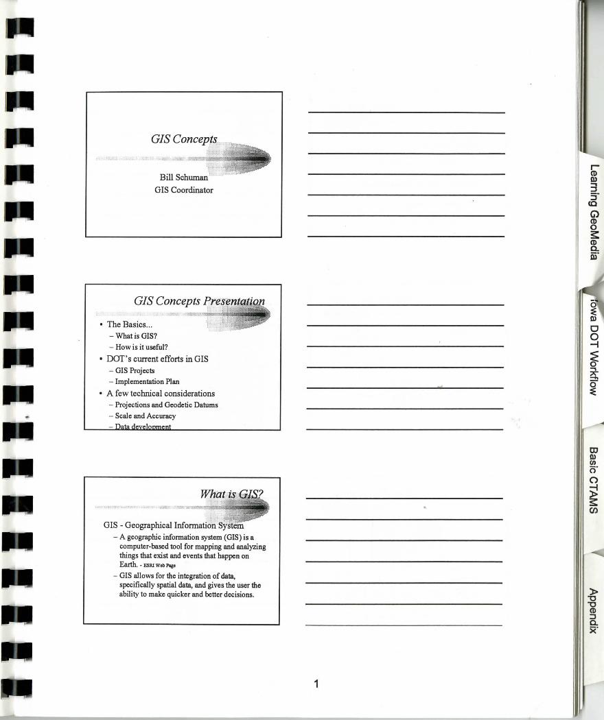
• The Basics ... - What is GIS?

- How is it useful?

• DOT's current efforts in GIS - GIS Projects

- Implementation Plan

• A few technical considerations -Projections and Geodetic Datums

- Scale and Accuracy

GIS - Geographical -A geographic information system (GIS) is a

computer-based tool for mapping and analyzing things that exist and events that happen on Earth. - ESRl Web P~~:c

- GIS allows for the integration of data, specifically spatial data, and gives the user the ability to make quicker and better decisions.

1

rCD ll)

3 :r co G) CD 0 s: CD a. iii'

OJ Q) en cr ()

~ s: (J)

)> "'0 "'0

CD :::1 a. )("

• Map - Representative model surface of the earth - Point.! (Water well, sign, accident, hydrant, ... )

- Linea (Road, river, stream, utility line, ... )

- Polygons (Wetland, city limits, soil boundaries, .. . )

• Database - Attribute storage software - GIS system information

- User attribute information

- Metadata- Data about data (projection, valid values, collection method, accuracy, etc.)

How

2 3

r(l) Q)

3 s(C

G) (l) 0 s:. (l) a. iii"

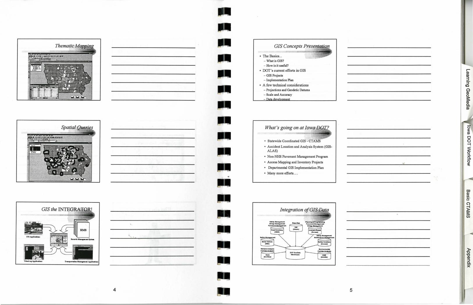
Tr•~p...udM M•..-•tA,pllmd••

4

GIS Concepts


- How is it useful?



• A few technical considerations - Projections and Geodetic Datums


What 's going on at

• Statewide Coordinated

• Accident Location and Analysis System (GIS-ALAS)

• Non-NHS Pavement Management Program

• Access Mapping and Inventory Projects

• Departmental GIS Implementation Plan

• Many more efforts ....

Integration

llfety MIMJM!ent 8r1ciJI MIMIMieftt

,.,Yemeni. I .. MQMtent

5

r(1) Q) ., ::J :r (C

G) (1) 0 s::. (1) a. iii"

)> -o -o (1) ::J a. x·

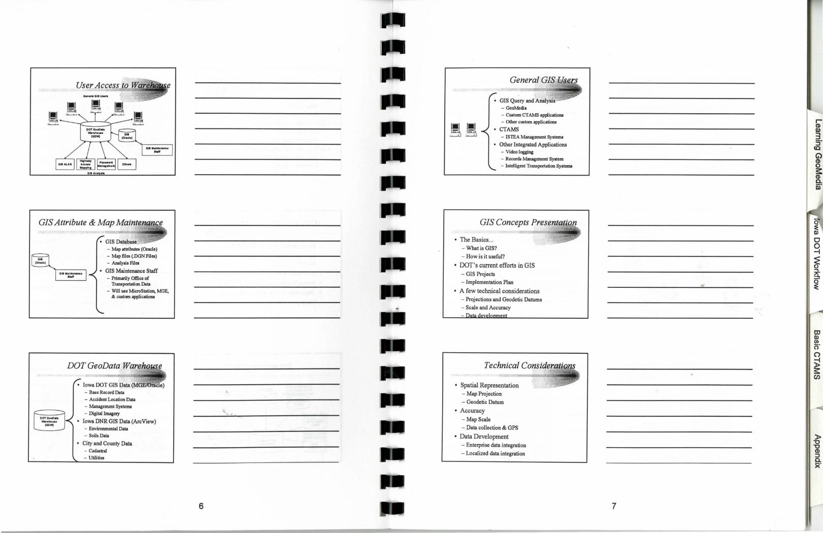
- Map attributes (Oracle) - Map files (DGN Files) - Analysis Flies

• GIS Maintenance Staff - Primarily Office of

Transportation Data - Will use MicroS tali on, MGE,

& custom applicatio111

- Base Record Data - Accident Location Data - Management Systeflll

- Digitallmagery

• Iowa DNR GIS Data (Arc View) - Environmental Data

- Soils Data

• City and County Data - Cadastral - Utilities

6

- GeoMcdia - Custom CTAMS applicati0111 - Other custom applicatio111

• CTAMS - IS TEA Management Systems

• Other Integrated Applications - Video logging

- Records Management System

- Intelligent Transportation Systems


- How is it useful?



• A few technical considerations - Projections and Geodetic Datums


Technical C

• Spatial Representation - Map Projection

- Geodetic Datum

• Accuracy - Map Scale

- Data collection & GPS

• Data Development - Enterprise data integration

- Localized data integration

7

r(1) ID 3 :r (Q

G) (1) 0 s: CD a. iii"

Map Projections &

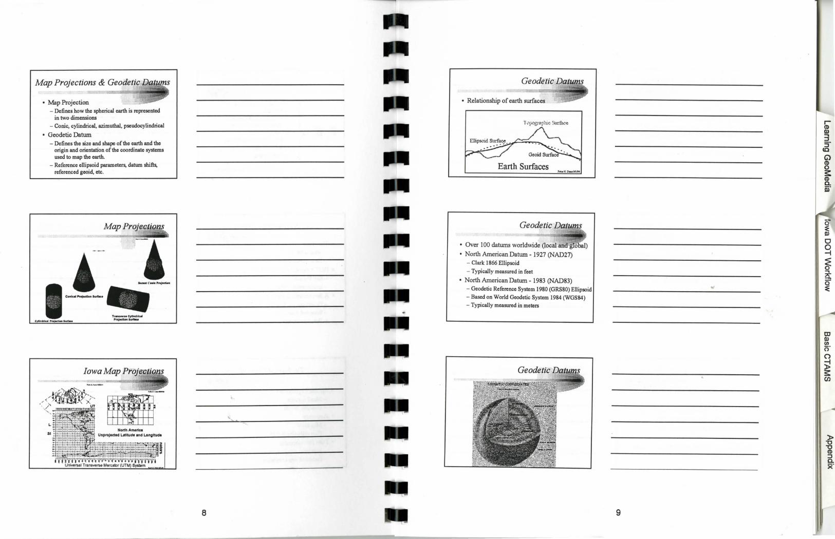
• Map Projection - Defines how the spherical earth is represented

in two dimensions

- Conic, cylindrical, azimuthal, pseudocylindrical

• Geodetic Datum - Defines the size and shape of the earth and the

origin and orientation of the coordinate systems used to map the earth.

- Reference ellipsoid parameters, datum shifts, referenced geoid, etc.

iTfi'fiTjTi'H'i''4'l"h'1''jTjT;•h·•;•·iTl''ITfl'Tfi'j UnM>rsal Transver5e Mercator (UTM) System •.

8

Earth Surfaces

• Over I 00 datwns wo,rld,wide a,oeii] • North American Datum - 1927 (NAD27)

- Clark 1866 Ellipsoid

- Typically measured in feet

• North American Datum - 1983 (NAD83) -Geodetic Reference System 1980 (GRS80) Ellipsoid

-Based on World Geodetic System 1984 (WGS84)

- Typically measured in meters

9

rCD Q)

3 :r (Q

G) CD 0 3: CD c. nr

tD Q) en cr ()

~ s: en

)> "'0 "'0

CD ::J c. x·

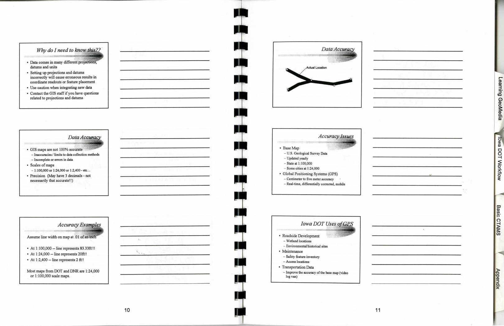
Why do I need to

• Data comes in many datums and units

• Setting up projections and datums incorrectly will cause erroneous results in coordinate readouts or feature placement

• Use caution when integrating new data

• Contact the GIS staff if you have questions related to projections and datums

GIS maps are not 100% acc:tm~lte ;;

- Inaccumcies I limits to data collection methods

- Incomplete or errors in data

• Scales of maps - 1:100,000 or 1:24,000 or 1:2,400- etc ...

• Precision (May have 3 decimals - not necessarily that accurate!!)

A

Assume line width on map at ' ·

• At 1:100,000 --line represents 83 .33ft!! I

• At 1:24,000 --line represents 20ft!!

• At 1:2,400 --line represents 2 ft! I

Most maps from DOT and DNR are 1 :24,000 or 1:100,000 scale maps.

10

qs

• Base Map - U.S. Geological Survey Data

- Updated yearly

- State at 1:100,000

- Some cities at 1 :24,000

• Global Positioning Systems (GPS) - Centimeter to five meter accumcy

- Real-time, differentially corrected, mobile

Iowa DOT

• Roadside Development - Wetland locations

- Environmental/historical sites

• Maintenance - Safety feature inventory

- Access locations

• Transportation Data

- Improve the accuracy of the base map (video log van)

11

rCD fl)

3 s(Q

G) CD 0 3: CD a. or

CD Q) en cr ()

~ s: (J)

)> "0 "0

CD :J a. x·

Why do I need to

• Data comes in many scales

• Understand the limitations of some data and remember the least-common-denominator

• Use caution when integrating new data, especially if not well documented (metadata)

• Contact the GIS staff if you have questions related map scales and data accuracy

Data

• Ask some questions ... - Do I need updated data from the GeoData

Warehouse on a regular basis - Does it need to closely integrate with the other

systems in the DOT?

- Could this data ever be used by anyone outside my office?

• YES- GeoData Warehouse

• NO - Do your own thing

Why should!

Questions? ,.

12 13

rCD Q)

3 sec G) CD 0 3: CD a. ii'i"

)> 'U 'U CD ::J a. x·

I I

... ...

14

rCD Q)

3 s

(Q

G) CD 0 s: CD a. nr

m Q) en (5"

0

~ s: en

+ GeoMedia Overview

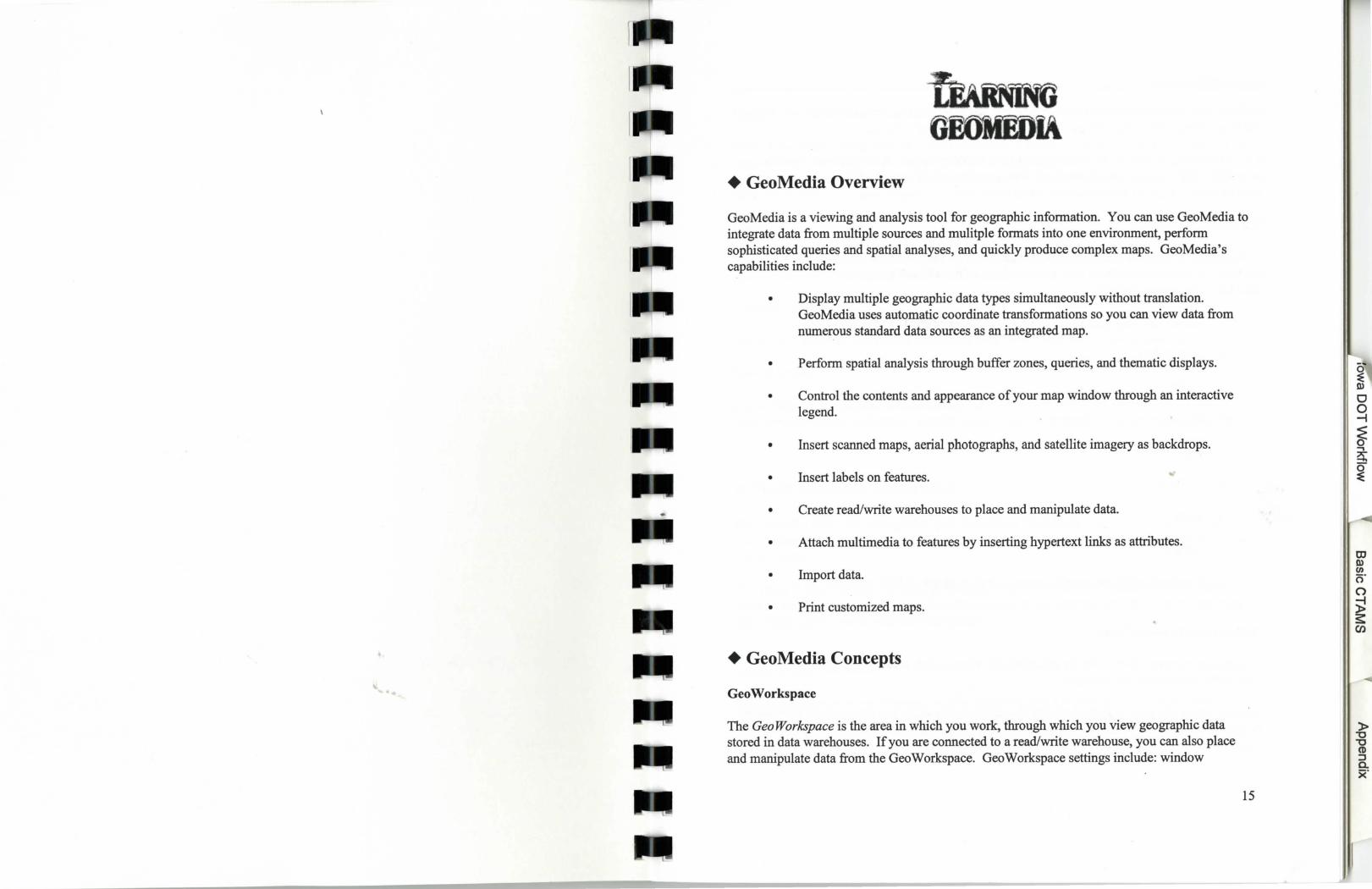
GeoMedia is a viewing and analysis tool for geographic information. You can use GeoMedia to integrate data from multiple sources and mulitple formats into one environment, perform sophisticated queries and spatial analyses, and quickly produce complex maps. GeoMedia's capabilities include:

• Display multiple geographic data types simultaneously without translation.

•

•

•

•

GeoMedia uses automatic coordinate transformations so you can view data from numerous standard data sources as an integrated map.

Perform spatial analysis through buffer zones, queries, and thematic displays .

Control the contents and appearance of your map window through an interactive legend.

Insert scanned maps, aerial photographs, and satellite imagery as backdrops .

Insert labels on features .

• Create read/write warehouses to place and manipulate data.

• Attach multimedia to features by inserting hypertext links as attributes.

• Import data .

• Print customized maps .

+ GeoMedia Concepts

Geo Workspace

The Geo Workspace is the area in which you work, through which you view geographic data stored in data warehouses. If you are connected to a read/write warehouse, you can also place and manipulate data from the GeoWorkspace. GeoWorkspace settings include: window

15

tD m en c=r ()

~ s: en

)> "0 "0 (1) ::J a. x·

Learning GeoMedia

configuration, coordinate system, queries, legends, thematic displays, menu settings, and warehouse connections. The file extension for a Geo Workspace is * .gws.

A GeoWorkspace Template is a starting point for a GeoWorkspace. A template can store the same settings (i.e. warehouse connections, views, queries, etc.) that a GeoWorkspace can store. The file extension for a GeoWorkspace Template is *.gwt.

Warehouse Connection

A Warehouse Connection is the source of geographic data accessed from a GeoWorkspace. Multiple warehouse connections may be made from within a GeoWorkspace. Available GeoMedia data servers include:

• Access (the only type of connection that can be opened as read/write)

• ARC/INFO

• Arc View

• CADD

• FRAMME

• MGDM

• MGE

• MGSM

• Oracle (SDO) (Data may be imported into an Oracle (SDO) warehouse.)

Features and Feature Classes

Afeature is represented on a map by geometry (i.e. a line, point, area, etc.) and is defined by nongraphic attributes in the database.

Features are categorized by feature classes (i.e. roads, bridges). A data set generally consists of several feature classes. The word feature refers to each occurance of a feature within a feature class. For example, Counties is a feature class, where as Story County is a feature.

16

Learning GeoMedia

Legend

The legend is the display control center for the map window. It controls which map objects are displayed and how they look. Map objects are displayed (in the active window) by adding them to the legend. Map objects and legend entries are linked-- manipulating a legend entry will modify the display of a map object.

Query

A query is a request for specific information such as features meet specified criteria. Query results can be shown in a map window or data window or both.

Attribute Query

An attribute query is a request to the database for information about one feature class.

Spatial Query

A spatial query is a request to the database for information about two feature classes and their spatial relationship to each other. Spatial queries may be further defined by attribute queries.

+ Start Learning GeoMedia!

This tutorial guides you through the basic features ofGeoMedia®, using the sample dataset of the United States that is delivered with GeoMedia to select possible locations for a ski resort in the United States.

This tutorial is sequential, you must go through the sections in order because the later sections build on earlier ones. Keep in mind that this tutorial shows only one workflow, although there are many possible workflows with GeoMedia.

Create a Geo Workspace

First, you create a new GeoWorkspace. The GeoWorkspace is the area in which you work, through which you view geographic data. If you are connected to a read/write warehouse, as explained in the next section, you can also place and manipulate data from the GeoWorkspace.

17

m Q) en cr 0

~ s:: Cll

)> "0 "0 CD ::J a. x·

Learning GeoMedia

1. Open OeoMedia.

2. Under the Create a New GeoWorkspace Using section, select Blank GeoWorkspace.

. The GeoWorkspace is created, and it is given the default name, GeoWorkspacel.

The OeoWorkspace contains the empty legend and the map window. The map window, which is titled Map Window I by default, is the window in which you view feature geometries, images, and labels.

Deiming the Coordinate System

A Oeo Workspace coordinate system defines how geographic data are displayed.. Data are transformed from the warehouse coordinate system to the Oeo Workspace coordmate system.

The default coordinate system for the OeoWorkspace is Cylindrical Equirectangular. However,

you will need to change it to US Standard.

1. Select View>GeoWorkspace Coordinate System from the menu bar.

2. On the GeoWorkspace Coordinate System dialog box, make sure the Storage Space tab is selected, and select Geographic as the Base storage type.

3. Select the Paper Space tab. In the Nominal map scale field, type or select from the drop-down list 5,000,000 (5 million).

4. Select the Geographic Space tab. In the Geodetic datum field, select United States

Standard from the drop-down list.

5. Click OK on the GeoWorkspace Coordinate System dialog box.

The coordinate system is changed to US Standard.

NOTE: The OeoWorkspace coordinate system must match the warehouse coordinate sy~tem when displaying raster images, FRAMME data, and ARC/INFO data. However, a coor_dmate system file (*.cs!J can be defined to convert the warehouse data to the workspace coordmate

system.

18

Learning GeoMedia

Saving the Geo Workspace

Before continuing, save the OeoWorkspace.

1. Select File>Save GeoWorkspace . 2. In the File name field, type the name learning. Click Save.

NOTE: Any time you exit this tutorial or OeoMedia, save the OeoWorkspace first.

+Using Warehouses to Connect to Data

Creating an Access Warehouse

Next, you create a warehouse to which you can write data. A warehouse is the source of geographic data for OeoMedia. Each warehouse contians only one type of geographic data, such as Access, MOE, FRAMME, MOE Segment Manager, ARC/INFO, Oracle, ArcView, or CADD.

For this project, you create an Access warehouse. An Access warehouse is the only type of warehouse you can create and write to through GeoMedia, although you can connect to any of the other types of warehouses.

1. Select Warehouse> New Warehouse.

The default template is Normal.mdt.

An Access Warehouse is the starting point for a new Access warehouse. A template must be used to create a new, empty warehouse.

2. Make sure the setting is Document and click OK.

3. In the File name field, type the name learning for the warehouse. Make sure Save as type is set to Access, and click Save.

The file is saved in the Warehouses directory as learning.mdb.

19

OJ Q) en cr 0

~ s: en

)> "0 "0 CD :J c. x·

Learning GeoMedia

Connecting to an Existing Access Warehouse

GeoMedia lets you connect to and display multiple geographic data types simultaneously without translation. For example, you could connect to an MGE warehouse, a FRAMME warehouse, and an ARC/INFO warehouse and view data from these different sources as an integrated map.

For this project, you will connect to another Access warehouse, USSampleData.mdb, and import some of its data into the Access warehouse you just created, /earning.mdb. Since you do not need all of the data contained in USSampleData.mdb, you import just the feature classes that you want to use.

In GeoMedia, a feature is a geographic entity represented on a map by geometry and defined by nongraphic attributes in the database. Afeature class is the classification to which each instance of a feature is assigned.

The sample US data set for this project contains feature classes such as States, Cities, and Interstates. For example, Minnesota is a feature in the States feature class, and Boston is a feature in the Cities feature class.

First, you connect to the warehouse from which you want to import data, USSamp/eData.mdb. This is the source warehouse.

20

1. Select Warehouse> New Connection.

The Warehouse Connection Wizard displays the different types of warehouses to which you can connect, such as MGE, FRAMME, and ARC/INFO.

2. Select Access, and click Next.

3. In the Define a connection name to access your Access warehouse field, delete the current text, and type Connection to US Data.

4. To select a GeoMedia database file, click Browse.

5. Select c:\Warehouses\USSampleData.mdb, and cliak Open.

6. Type this description: us Data, and click Next.

7. Make sure that the option Access all features in the warehouse is selected, and click Next.

Learning GeoMedia

8. Keep the option Let the wizard open the connection as read only and click Finish.

9. To verify that the connections to both warehouses are present, both the one you created and the source, select Warehouse > Edit Connection.

10. Click Close after verifying that both connections are listed.

Importing Data from an Access Warehouse

To import data means to copy data from a source warehouse to a target warehouse. You can import data from any GeoMedia-supported warehouse to an Access warehouse. Importing data to an Access warehouse allows you to place, move, edit, and delete features.

1. Select Warehouse> Import from Warehouse.

2. Read the instructions on the Import Warehouse Wizard dialog box, and click Next. The source warehouse is Connection to US Data (USSamp/eData.mdb), and the target warehouse is /earning.mdb.

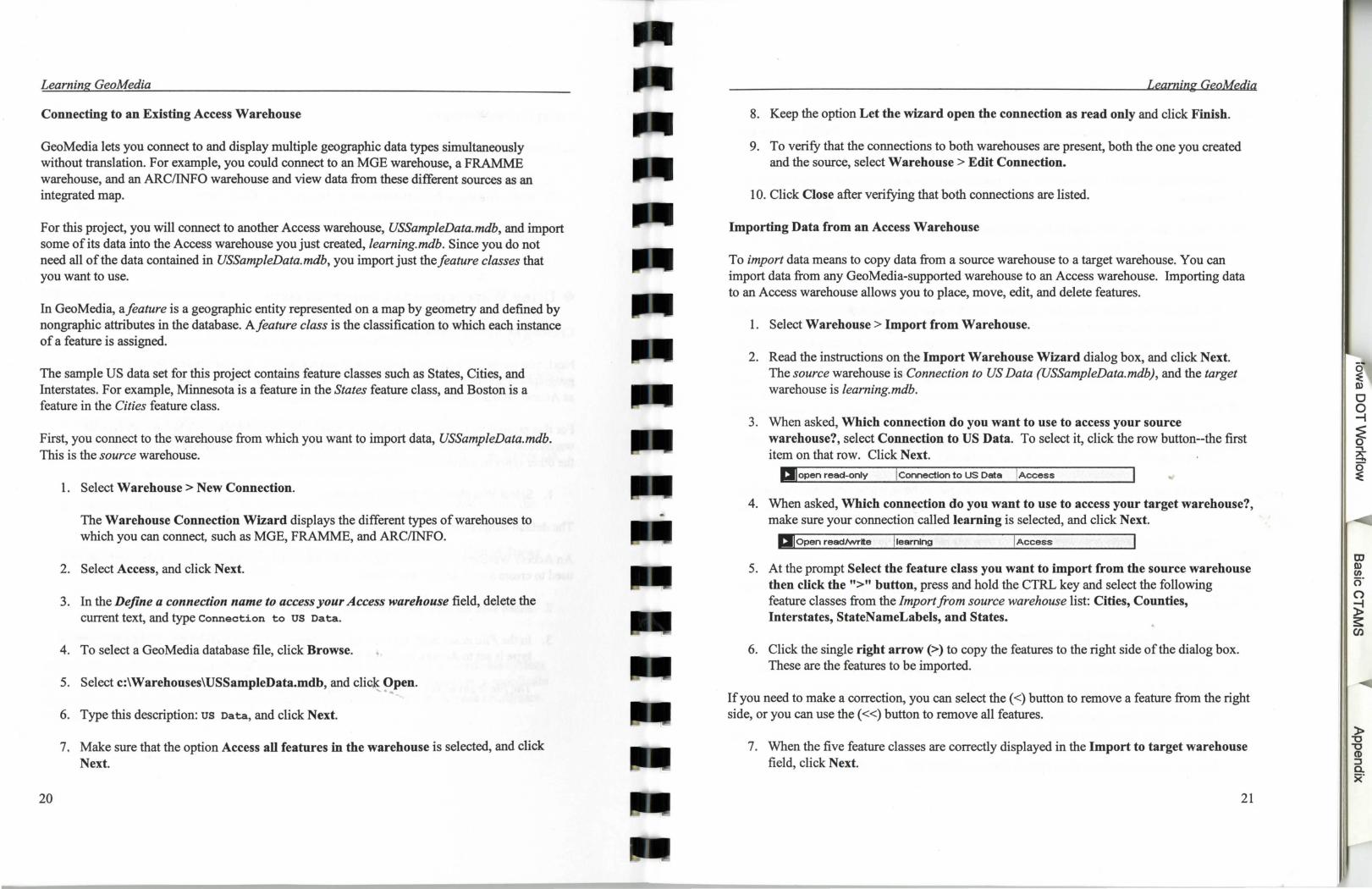
3. When asked, Which connection do you want to use to access your source warehouse?, select Connection to US Data. To select it, click the row button--the first item on that row. Click Next.

aJ open read-only J Connection to US Data J Access

4. When asked, Which connection do you want to use to access your target warehouse?, make sure your connection called learning is selected, and click Next.

aJ Open read/write Jlearnlng !Access

5. At the prompt Select the feature class you want to import from the source warehouse then click the">" button, press and hold the CTRL key and select the following feature classes from the Import from source warehouse list: Cities, Counties, Interstates, StateNameLabels, and States.

6. Click the single right arrow(>) to copy the features to the right side of the dialog box. These are the features to be imported.

If you need to make a correction, you can select the ( <) button to remove a feature from the right side, or you can use the(<<) button to remove all features.

7. When the five feature classes are correctly displayed in the Import to target warehouse field, click Next.

21

Learning GeoMedia

8. Change the name of the StateNameLabels feature class to StateN ames by clicking the field and typing in the new name (do not use spaces within the name). Do not change the name of the States feature class. Click Next.

9. When asked What do you want to do?, make sure Create new legend entries option is

selected.

10. Select Active Map Window (MapWindowl) to display the feature classes in this map window, and click the(>) button.

11. Click Finish.

The Import Statistics dialog box appears, and the message Importing ... appears as the features are imported for each feature class. This may take a few minutes. As each feature class is imported, the status bar indicates the progress, and then the number of features that have been imported is shown for that feature class. When both feature classes have been imported, the message Import complete appears.

12. Click Close.

The features appear in the map window. You should see a map of the United States with Cities, Counties, Interstates, StateNames, and States.

13. If you do not see the entire map in your window, make the window larger and then select

View> Fit All.

Deleting a Connection

Since you have imported data to your own Access warehouse, you no longer need the connection to USSampleData.mdb, and can delete this connection.

22

1. Select the Warehouse>Edit Connection.

2. In the Warehouse Connections dialog box, on the row for the Connection to US Data, click inside the Status column. 1..

·~

The entry highlights, indicating that it is currently selected, and then a down arrow appears. This indicates a drop-down list.

To close the connection, select closed from the Status pull-down menu.

Learning GeoMedia

3. On the Warehouse Connections dialog box, select the row button for the connection named Connection to US Data.

The row highlights.

4. Click Delete to delete this connection. Answer OK to Do you really want to remove this connection?

5. Click Close.

+ Working with the Legend

The legend is the interactive control center that determines what is displayed in the map window. Through the legend, you control which map elements--such as feature classes, images, query results, and thematic displays--are displayed in the map window and how they look. A separate entry exists for each map object. Each entry contains, at minimum, a title and graphical representation of the map object.

1. The legend should be display~d in the map window. If it is not, select View>Legend to tum it on.

The map is somewhat crowded with so much displayed in it. You just want to look at states for now, so you do not want some of the other information to display.

2. Select Legend > Properties. On the row for the Cities entry, click inside the Display column.

The entry highlights, indicating that it is currently selected, and then a down arrow appears. This indicates a drop-down list.

3. Click the down arrow, and select Off. Click OK to dismiss the dialog box.

The entry for Cities is still on the legend, but the entry is dimmed and the cities are no longer displayed on the map.

Now you will remove another entry from the legend, Counties. Rather than repeating the process above, you will use a shortcut.

23

to fl) en cr 0

~ s:: en

)> "0 "0 ([) ::J c. x·

Learning GeoMedia

4. Place your cursor over the Counties entry on the legend, and click on the right mouse button. Click Display Off to turn off the counties.

5. Repeat the previous step to remove the interstates from the map.

Only the states and state names should be displayed. However, the state names are too small to read, so you will need to make them bigger.

24

6. Select Legend> Properties, from the menu bar or from the toolbar.

7. Select the entry (row) for StateN ames by clicking the row selector button.

a A IS1ateNames lon ~ ..,

8. Click the Style button at the lower right comer of the Entries tab. On the Style Definition dialog box, select a font size of 48-points by clicking the drop-down arrow in the Size field, and selecting 48. Select Bold, and click OK.

9. With the StateNames row still selected, click in the Display cell for that row. Click the drop-down list to open it, and scroll down and select the By Scale option.

10. Click the Scale button.

The Scale Range dialog box lets you set a scale at which graphics are displayed. When the map window scale falls within the scale range of a legend entry and Display is set to By Scale, the graphics are displayed; otherwise, the graphics are not displayed.

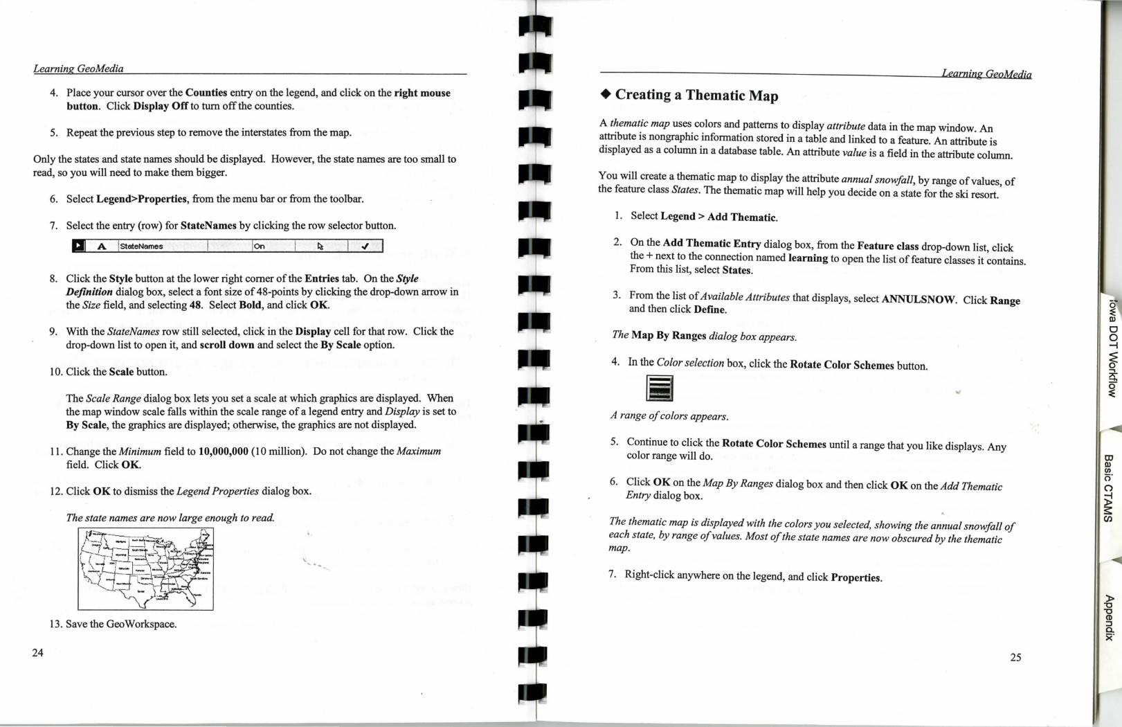
11. Change the Minimum field to 10,000,000 (1 0 million). Do not change the Maximum field. Click OK.

12. Click OK to dismiss the Legend Properties dialog box.

The state names are now large enough to read.

...

13. Save the GeoWorkspace.

Learning GeoMedia

+ Creating a Thematic Map

A thematic map uses colors and patterns to display attribute data in the map window. An attribute is nongraphic information stored in a table and linked to a feature. An attribute is displayed as a column in a database table. An attribute value is a field in the attribute column.

You will create a thematic map to display the attribute annual snowfall, by range of values, of the feature class States. The thematic map will help you decide on a state for the ski resort.

1. Select Legend > Add Thematic.

2. On the Add Thematic Entry dialog box, from the Feature class drop-down list, click the + next to the connection named learning to open the list of feature classes it contains. From this list, select States.

3. From the list of Available Attributes that displays, select ANNULSNOW. Click Range and then click Defme.

The Map By Ranges dialog box appears.

4. In the Color selection box, click the Rotate Color Schemes button.

A range of colors appears.

5. Continue to click the Rotate Color Schemes until a range that you like displays. Any color range will do.

6. Click OK on the Map By Ranges dialog box and then click OK on the Add Thematic Entry dialog box.

The thematic map is displayed with the colors you selected, showing the annual snowfall of each state, by range of values. Most of the state names are now obscured by the thematic map .

7. Right-click anywhere on the legend, and click Properties.

25

)> "0 "0 CD ::J a. x·

Learning GeoMedia

8. On the Legend Properties dialog box, select the entry for StateNames (click the row selector for that row), and select the topmost Priority arrow to move StateN ames to the

top of the list. Click OK to dismiss the dialog box.

The state names again appear in the map window because they are now displayed above all of the other legend entries.

9. Save the Geo Workspace.

+ Creating Queries and Buffer Zones

A query is a request for information. When you display a query, you are requesting to see features that meet specific criteria. With GeoMedia, you can build a query by making selections on a dialog box, without needing to know SQL. Queries present current information in the warehouse. This means that each time you display a query, you get the current information in the warehouse.

A buffer zone is a user-defined region around or within one or more features. You can buffer zone geometry for a feature class or the results of a query.

Build a Query

Next you create an attribute filter query, which lets you search the database for a specific value or a range of values for one attribute or a combination of attributes that apply to one feature class. The feature you query will be States.

First you will change a couple of options.

1. Select Tools>Options.

2. Select the Measurement tab. . ...

3. In the Distance field, select mi from the drop-down list to set the ground units to miles.

4. Select the Query tab.

26

Learning GeoMedia

5. Uncheck the option, Confrrm show value operations.

6. ClickOK

Now, you want to see which states have a relatively high annual snowfall and a low temperature. These would be good candidates for a ski resort.

1. Select Tools> New Query to display the New Query dialog box.

2. From the Select Features in drop-down list, open the connection named learning. From this list, select States.

3. Click the Filter button to display the dialog box that lets you define afilter for States.

You specify which features you want to find by defining a filter. Think of an attribute filter query as a sentence. A filter would be the same as a ''where" clause (find all schools where enrollment is less than 400).

4. Select ANNULSNOW (annual snow) from the list of attributes.

5. Click the down arrow (pictured below) beneath the Attributes field.

[3 6. Select the greater than(>) operator.

The attribute and operator appear in the Filter field at the bottom of the dialog box. You can also type SQL statements directly into this field.

7. Click the Show Values button.

8. From the list of values that appears, select 40 (or, you could type this value directly into the expression box) and click the down arrow below the Values field.

The expression ANNULSNOW > 40 is displayed in the Filter field.

9. Select the AND operator.

10. Select the A VETEMP (average temperature) attribute, and click the down arrow beneath the list.

11. Select the less than (<) operator.

27

Learning GeoMedia

12. Type the value 50 at the end ofthe query expression in the Filter field.

The expression ANNULSNOW > 40 AND A VETEMP < 50 should be displayed in the Filter field.

13. Click OK on the States Filter dialog box.

14. In the Name field in the New Query dialog box, delete the text Queryl and type States

by Snow/avetemp. It is always a good idea to give your queries a descriptive name, as it is easier for you to select the query by a meaningful name.

Named queries are very useful, as you can rerun them at any time, display them in other map or data windows, or use them as input to other queries.

15. For a description, type States where annual snow > 40 and average temperature

<50.

16. Click OK to run the query and dismiss the New Query dialog box.

The query is added to the legend. The legend entry for the query contains the style key that shows the color of the query results on the map which are shown as states outlined in a different color.

Changing the Style of Map Objects

The Style Defmition dialog box lets you change the appearance of a map object--such as feature classes, images, query results, and thematic displays.

1. Turn offthe display of the thematic map by right-clicking its legend entry, States by ANNULSNOW, and selecting Display Off.

2. Take the entry for the thematic map off of the legend, by right-clicking its legend entry, States by ANNULSNOW, and selecting Hide Legend Entry.

NOTE: Although the thematic map is currently not display® on the legend or on the map, it can be redisplayed by selecting Legend > Properties and clicking· in the Entry column in its row to display it on the legend, and by setting the value in the Display field to On to display it on the map. For now, leave it turned off in both places.

28

Learning GeoMedia

The thematic map is no longer displayed, but it still may be difficult to see the results of the query you just ran, although those states are outlined in a different color. To better see the query results, you can change the style.

3. To change the style, use a shortcut: double-click the style key( see arrow below) on the legend for the query entry States by Snow/avetemp.

I QStates by Snow/avetemp I 74

The Style Defmition dialog box appears. The Area Boundary tab shows the color, weight, and line style for the boundary of the item.

4. Select the Area Fill tab. From the Type drop-down list in the primary fill box, select Solid.

5. Select a primary fill color you want by selecting the Color button and picking a color, such as light blue.

6. Click OK to dismiss the Color dialog box.

7. From the Pattern drop-down list, select a pattern, such as Trellis.

An example of the pattern appears in the Sample area.

8. Choose another Cross-hatch color if you want.

9. Click OK when you have a pattern and colors you want.

The results of the query States by Snow/avetemp appear on the map in the colors and pattern you selected.

10. The state names are covered by the query results. You can use a shortc~t to change the priority of the state names so they appear over the query results. Select the entry for StateN ames on the legend, continuing to hold the mouse button down, and use the mouse cursor to drag this entry to the top of the legend.

The state names appear over the patterned area.


29

CD ru (f)

cr 0

~ s:: CJl

)> "C "C (1) ::J a. .x·

Learning GeoMedia

Deime a Connection Filter

A connection filter defines an area in your map window. When you apply a connection filter to a warehouse, only features in the defined area are displayed and accessible when you add them to the map window. Connection filters only impact feature classes added after the filter was applied. Connection filters are optional, but you define one in this project to see the features in only two states.

For example, suppose you decide to focus on only the states of Minnesota and Wisconsin for possible ski resorts.

1. From the menu bar, select View > Zoom > In.

You will zoom in on a mid-west region of the United States.

30

2. Place the zoom-in pointer above the middle of the state of North Dakota. Press and hold the left mouse button, and drag the cursor to the bottom of the right edge of the state of Ohio, and then release the left button.

The view is zoomed in on.

3. Press ESC to exit the Zoom command.

4. Select Warehouse> Deime Connection Filter.

5. In the Filter name field, type Minnesota and Wisconsin.

6. Keep the Spatial operator, Overlap, and the placement option, Create a new il.lter by placing a two point area. " ....

7. Click Deime.

The cursor changes to a crosshair.

Learning GeoMedia

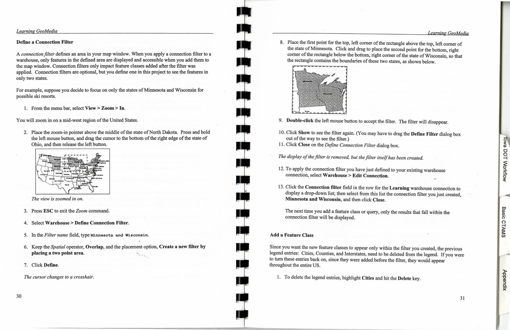
8. Place the first point for the top, left corner of the rectangle above the top, left corner of the state of Minnesota. Click and drag to place the second point for the bottom, right corner of the rectangle below the bottom, right corner of the state ofWisconsin, so that the rectangle contains the boundaries of these two states, as shown below.

9. Double-click the left mouse button to accept the filter. The filter will disappear.

10. Click Show to see the filter again. (You may have to drag the Deime Filter dialog box out of the way to see the filter.)

11. Click Close on the Define Connection Filter dialog box.

The display of the filter is removed, but the filter itself has been created.

12. To apply the connection filter you have just defined to your existing warehouse connection, select Warehouse> Edit Connection.

13. Click the Connection f"tlter field in the row for the Learning warehouse connection to display a drop-down list; then select from this list the connection filter you just created, Minnesota and Wisconsin, and then click Close.

The next time you add a feature class or query, only the results that fall within the connection filter will be displayed.

· Add a Feature Class

Since you want the new feature classes to appear only within the filter you created, the previous legend entries: Cities, Counties, and Interstates, need to be deleted from the legend. Ifyou were to turn these entries back on, since they were added before the filter, they would appear throughout the entire US.

I. To delete the legend entries, highlight Cities and hit the Delete key.

31

OJ Q) en cr ()

~ s:: en

Learning GeoMedia

2. Answer yes to the question, Delete Legend Entires?

3. Repeat the previous two steps for the Counties and Interstates entries.

You will now add three feature classes from your warehouse to display and query.

1. Select Legend > Add Feature Class.

2. On the Add Feature Class Entry dialog box, make sure the Learning connection is selected.

3. Hold down the CTRL key and select Cities, Counties, and Interstates from the list of feature classes.

4. Click OK.

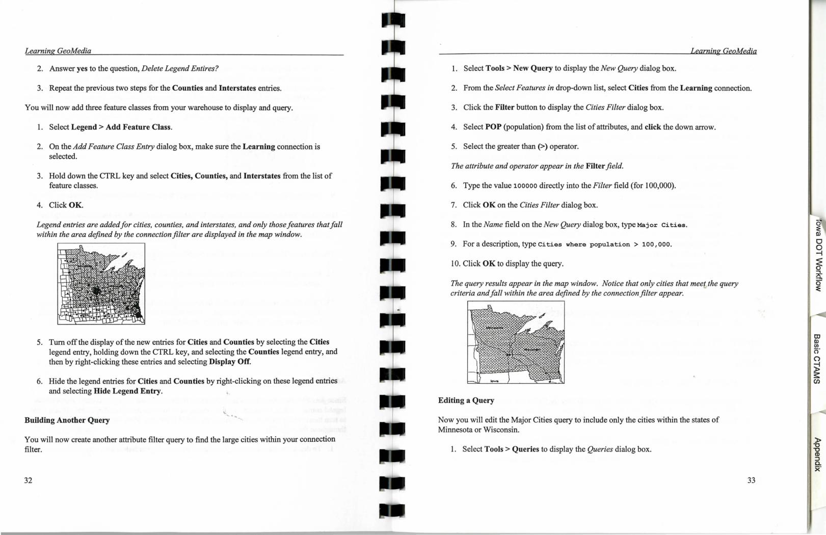
Legend entries are added for cities, counties, and interstates, and only those features that fall within the area defined by the connection filter are displayed in the map window.

5. Tum off the display of the new entries for Cities and Counties by selecting the Cities legend entry, holding down the CTRL key, and selecting the Counties legend entry, and then by right-clicking these entries and selecting Display Off.

6. Hide the legend entries for Cities and Counties by right-clicking on these legend entries and selecting Hide Legend Entry.

Building Another Query

You will now create another attribute filter query to find the large cities within your connection filter.

32

Learning GeoMedia

1. Select Tools > New Query to display the New Query dialog box.

2. From the Select Features in drop-down list, select Cities from the Learning connection.

3. Click the Filter button to display the Cities Filter dialog box.

4. Select POP (population) from the list of attributes, and click the down arrow.

5. Select the greater than(>) operator.

The attribute and operator appear in the Filter field.

6. Type the value 100000 directly into the Filter field (for 1 00,000).

7. Click OK on the Cities Filter dialog box.

8. In the Name field on the New Query dialog box, type Major Cities.

9. Fora description, type cities where population> 100,000.

10. Click OK to display the query.

The query results appear in the map window. Notice that only cities that meet the query criteria and fall within the area defined by the connection filter appear.

Editing a Query

Now you will edit the Major Cities query to include only the cities within the states of Minnesota or Wisconsin.

1. Select Tools > Queries to display the Queries dialog box.

33

tD Q) en cr ()

~ s: CJ)

Learning GeoMedia

2. From the list of queries, select Major Cities, and then click Edit.

3. On the Edit Query dialog box, click Filter.

4. On the Cities Filter dialog box, click inside the Filter field, just after the string to be edited, POP> 100000.

5. Click the AND operator. Then, click the parentheses 0 operator.

6. Move the insertion point inside the parentheses. Then select from the attributes list in the following order:

- The STATE NAME attribute - The down arrow -The equal(=) operator - Show Values. - MINNESOTA from the list of values - The down arrow - The OR operator - The STATE NAME attribute - The down arrow - The equal ( =) operator -WISCONSIN from the list of values - The down arrow

The textshouldreadPOP> 100000 AND (STATE_NAME ='MINNESOTA' OR STATE_NAME ='WISCONSIN').

IMPORT ANT: Take a minute to verify that the text in the Filter field matches the text shown above. If it does not match, you may not obtain the correct results in the remainder of this tutorial.

7. Click OK to dismiss this dialog box.

The query is updated in the Filter field in the Edit Query dialog box.

8. Edit the Description field to add the text in Minnesota. and Wisconsin.

9. Click OK to run the query.

34

Learning GeoMedia

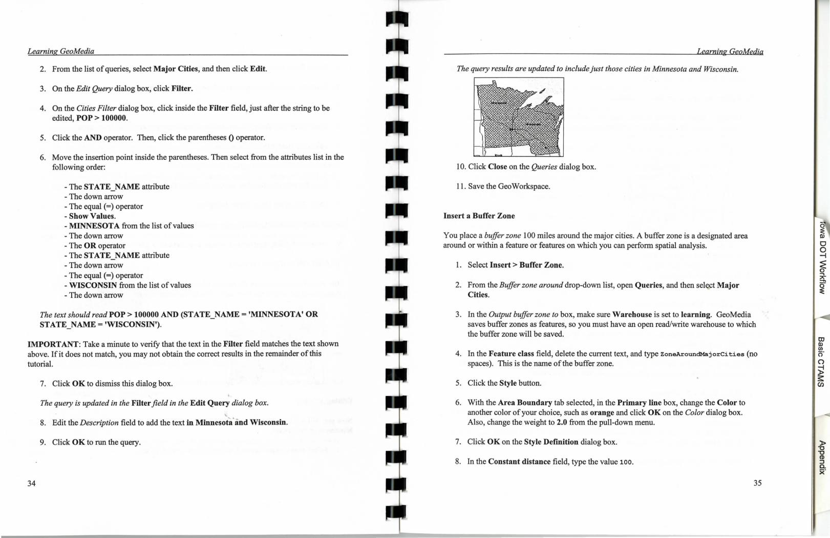
The query results are updated to include just those cities in Minnesota and Wisconsin.

10. Click Close on the Queries dialog box.


Insert a Buffer Zone

You place a buffer zone 100 miles around the major cities. A buffer zone is a designated area around or within a feature or features on which you can perform spatial analysis.

1. Select Insert > Buffer Zone.

2. From the Buffer zone around drop-down list, open Queries, and then select Major Cities.

3. In the Output buffer zone to box, make sure Warehouse is set to learning. GeoMedia saves buffer zones as features, so you must have an open read/write warehouse to which the buffer zone will be saved.

4. In the Feature class field, delete the current text, and type ZoneAroundMajorCities (no spaces). This is the name of the buffer zone.

5. Click the Style button.

6. With the Area Boundary tab selected, in the Primary line box, change the Color to another color of your choice, such as orange and click OK on the Color dialog box. Also, change the weight to 2.0 from the pull-down menu.

7. Click OK on the Style Def"mition dialog box.

8. In the Constant distance field, type the value 100.

35

OJ Ill en cr ()

~ s: C/l

)> "0 "0 CD :l a. )("

Learning GeoMedia

9. Make sure the Point buffer type is set to Single, and select the Merged option to create a merged buffer zone. Click OK.

The buffer zones appear in the map window.

10. To make it easier to see the buffer zones, turn off the display of the query, States by Snow/avetemp, by right-clicking this legend entry and selecting Display Off.

11. Hide the legend entry by right-clicking States by Snow/avetemp on the legend and selecting Hide Legend Entry.


Building a Query Using a Buffer Zone

You will create two more queries. These queries will be spatial queries, which request information from the database about two feature classes or queries based on their spatial relationships to each other.

The first query will let you find all sparsely populated counties that fall within the buffer zone you just created. These counties may be good candidates for a ski resort.

36

1. Select Tools> New Query.

2. From the Select Features in drop-down list, select Coni! ties from the Learning connection.

3. Click Filter to display the Counties Filter dialog box.

4. Select POP (Population) from the list of attributes, and click the down arrow.

Learning GeoMedja

5. Select the less than(<) operator.

6. Type the value 30000 directly into the Filter field (for 30,000).

7. Click OK on the Counties Filter dialog box.

8. Click the Spatial button on the New Query dialog box.

9. In the That field, select are contained by from the drop-down list.

10. In the Features in field, select the buffer zone you just created, ZoneAroundMajorCities, from the learning connection in the drop-down list.

11. In the Name field, type Small Counties Around Major Cities.

12. For a description, type Counties around major cities where population < 30,000.

13. Click OK to run the query.


Build a Query on a Query

You now build another query to find all counties from your previous query that are within 10 miles of an interstate.

1. Select Tools> New Query to create your final query.

37

Learning GeoMedia

38

2. From the Select Features in drop-down list, open Queries, and select the query you just created, Small Counties Around Major Cities.

3. Click Spatial.

4. In the That field, select are within distance of from the drop-down list.

5. Enter the value 10 for 10 miles in the Distance field.

6. In the Features in field, select the Interstates feature class from the Learning entry in the drop-down list.

7. Name this query Final Counties.

8. For a description, type Small counties around major cities within 10 miles of

an interstate.

9. Click OK to display the query.

The query results are displayed in the map window, but it is difficult to see the results since the results of the query Small Counties Around Major Cities are also displayed.

10. Turn off the display of this other query so that you can better see the results of the Final Counties query. (Right click on Small Counties Around Major Cities and select Display Off.)

11. Hide the legend entry by right-clicking on Small Counties Around Major Cities and selecting Hide Legend Entry.

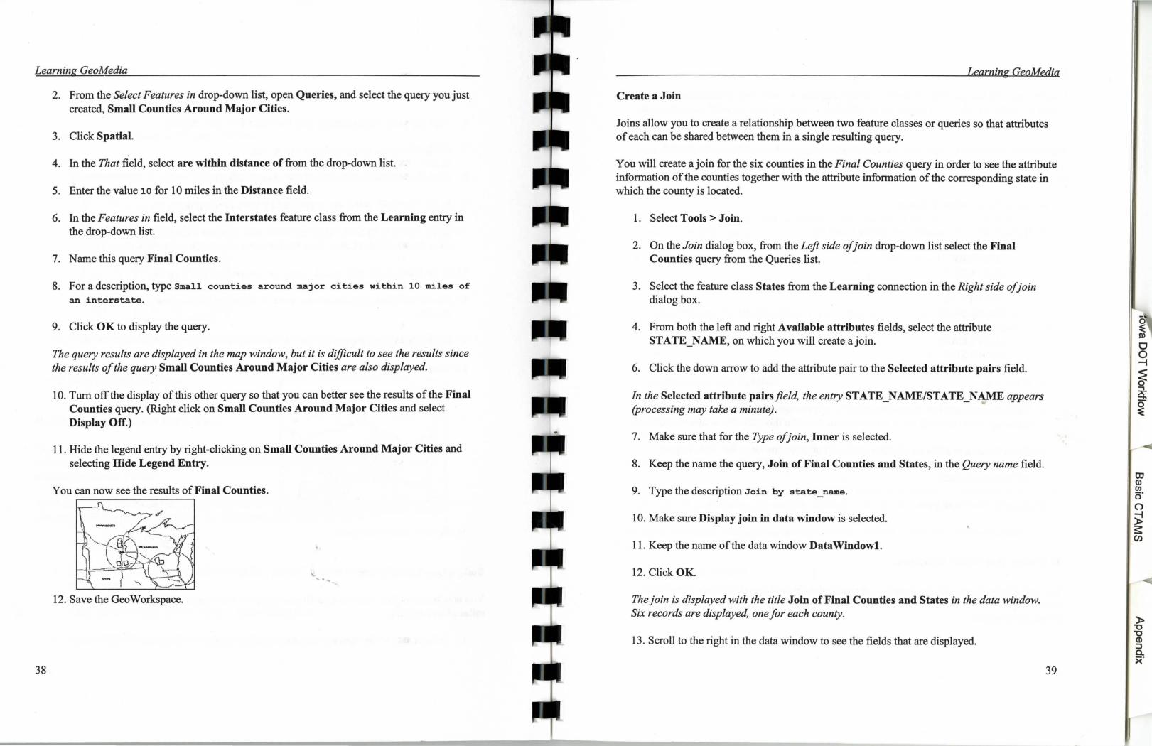
You can now see the results of Final Counties.

... 12. Save the GeoWorkspace.

Learning GeoMedia

Create a Join

Joins allow you to create a relationship between two feature classes or queries so that attributes of each can be shared between them in a single resulting query.

You will create a join for the six counties in the Final Counties query in order to see the attribute information of the counties together with the attribute information of the corresponding state in which the county is located.

1. Select Tools >Join.

2. On the Join dialog box, from the Left side ofjoin drop-down list select the Final Counties query from the Queries list.

3. Select the feature class States from the Learning connection in the Right side ofjoin dialog box.

4. From both the left and right Available attributes fields, select the attribute STATE_NAME, on which you will create ajoin.

6. Click the down arrow to add the attribute pair to the Selected attribute pairs field.

In the Selected attribute pairs field, the entry STATE_NAME/STATE_NAME appears (processing may take a minute).

7. Make sure that for the Type ofjoin, Inner is selected.

8. Keep the name the query, Join of Final Counties and States, in the Query name field.

9. Type the description Join by state_name.

10. Make sure Display join in data window is selected.

11. Keep the name of the data window Data Windowl.

12. Click OK .

The join is displayed with the title Join of Final Counties and States in the data window. Six records are displayed, one for each county.

13. Scroll to the right in the data window to see the fields that are displayed.

39

Learning GeoMedia

Data is displayed first for each of the six counties, and then for each county's state. Some of the attributes for the state have a 1 appended to the column name, to indicate a difference from the county attribute of the same name.

Suppose you wanted to compare the weather conditions (annual snowfall, annual rainfall, and average temperature) of each county to those of the county's state. To do this, you can specify the columns you do not want to be displayed.

14. Select Data > Show Columns.

15. Uncheck all ofthe columns except the following:

-AVETEMP -ANNULRAIN -ANNULSNOW -COUNTYID -STATE NAMEl -AVETEMPl - ANNULRAINl - ANNULSNOWl

16, Click OK

17. Scroll the data window to see that only the columns that you selected now appear, allowing you to see only the information you want (in this case, the weather conditions).

18. Close the data window by clicking on the X button on the menu bar with the gray background (the X on the blue background will close the GeoWorkspace). Keep the map window maximized.


+Using the Data Window \.

You will display a data window to look at the attributes for each county that you found with your last query, Final Counties. A data window is a view, in table format, of the nongraphic attributes of features.

40

Learning GeoMedia

Open a Data Window

1. Select Window> New Data Window.

2. In the New Data Window dialog box, keep DataWindowl for the name of the window, and select Final Counties from the Queries connection.

3. Click OK.

The data window appears, with six entries corresponding to the six counties that meet the requirements of the query.

4. To better see the map and data windows, select Window> Tile Horizontally.

5. Make the Map Window active by clicking on it once.

6. Select View>> Fit All, then select View>> Zoom>> ln. Click in the upper left hand comer of Minnesota and drag the box to the lower right hand comer ofWisconsin. Then select ESC.

7. To display the entries in the data window by state, select the STATE_NAME column heading and it will highlight.

8. Select Data > Sort Ascending.

The entries are sorted by state name.

9. Select any entry in the data window by clicking on the row selector for a row.

Notice that the corresponding County highlights in the map window. Conversely, if you select a state in the map window, the entry is highlighted in the data window.

This also demonstrates that you can use either a map window or a data window to select a feature from the database.

10. Close DataWindowl.

41

tD II> en cr ()

~ s: (J)

)> 'U 'U CD ::J a. S("

Learning GeoMedia

+ Placing Labels and Images

Labels in GeoMedia may be composed of text that you type and one or more attribute values derived from values stored in the warehouse.

Before placing labels, several steps will be performed to get the map window the way you want it.

Remove the Connection Filter

The connection filter you defined is no longer needed, so you can remove it.

1. Select Warehouse> Edit Connection.

2. Click the Connection filter column in the row for the Learning connection to display a drop-down list, and then scroll down to select the blank area in the list.

3. When the filter name no longer appears in the Connection filter column, the filter is removed from the warehouse connection.

4. Click Close.

5. On the legend, turn off the display of the state names by right-clicking the legend entry and selecting Display Off.

When you create your final output, you do not need the state names to appear on the United States map.

6. Select View > Fit All.


Name the Legend

You now name the legend for the US map. Naming a legend lets you apply it to another map in the same Geo Workspace. Assuming you have the same featlke classes, the feature classes will be displayed with the symbology from the named legend.

1. Select Legend > Name Legend.

42

Learning GeoMedia

2. In the Name field, type LearningLegendl .

3. Click OK.

Manipulate the View

You create another new map window in which you display a closer view of your results. In the new map window, you zoom in on the states of Minnesota and Wisconsin, which is the area that contains the results of the Final Counties query. Then you place labels for these counties.

Before opening the new map window, you can give your current map window a more descriptive name.

1. Select Window > Map Window Properties.

2. In the Map window name field, type us Map.

3. Click OK.

4. Select Window> New Map Window to open another map window.

5. In the New Map Window dialog box, name the new map window Final Counties.

6. Select LearningLegendl.

7. Click OK.

The new map window, Final Counties, is displayed.

8. Select Window> Cascade to see the two windows.

9. With the US Map window active, select View> Fit All.

In the next section, when you create the final output in Imagineer™ Technical, you will place a map view in a frame using the Fit to Frame option to size the map view to the frame. You first need to make sure that the map view is displayed appropriately in GeoMedia. Since you will display the entire view in the frame, you fit the view in the map window now.

10. Maximize the Final Counties window.

43

m ll) en ()' ()

~ s: en

)> "0 "0 CD :J a. .x·

Learning GeoMedia

11 . Turn on the display of the state names in the Final Counties map window by rightclicking the legend entry and selecting Display On.

12. Select View > Zoom > In.

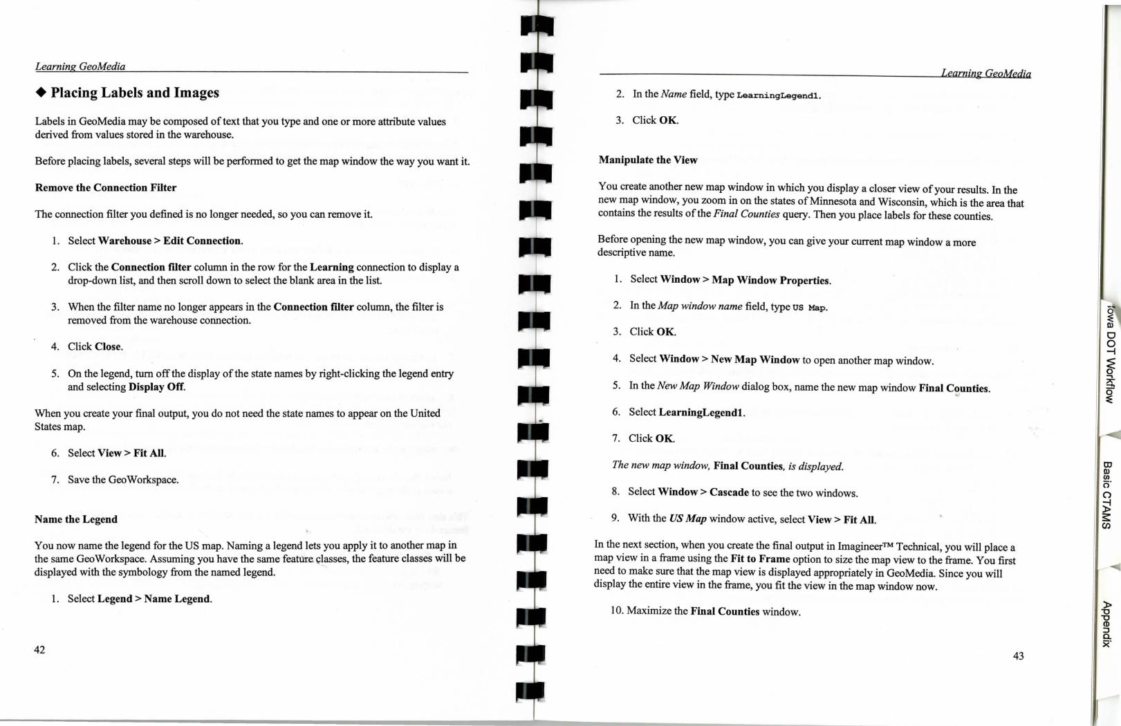
13. Place the zoom-in pointer at the top-left comer of the state of Minnesota.

14. Press and hold the left mouse button, and drag the cursor to the bottom-right comer of Wisconsin.

15. Release the left button.

The view is zoomed in on.

You should see four counties in Minnesota to the left, and two counties in Wisconsin to the right.

16. Hide the legend by double-clicking the legend icon on the legend title bar in order to better see all six counties.

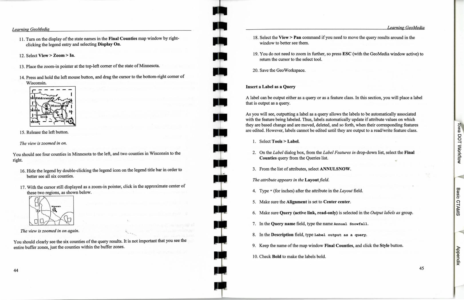
17. With the cursor still displayed as a zoom-in pointer, click in the approximate center of these two regions, as shown below.

The view is zoomed in on again. \. .......

You should clearly see the six counties of the query results. It is not important that you see the entire buffer zones, just the counties within the buffer zones.

44

Learning GeoMedia

18. Select the View> Pan command if you need to move the query results around in the window to better see them.

19. You do not need to zoom in further, so press ESC (with the GeoMedia window active) to return the cursor to the select tool.


Insert a Label as a Query

A label can be output either as a query or as a feature class. In this section, you will place a label that is output as a query.

As you will see, outputting a label as a query allows the labels to be automatically associated with the feature being labeled. Thus, labels automatically update if attribute values on which they are based change and are moved, deleted, and so forth, when their corresponding features are edited. However, labels cannot be edited until they are output to a read/write feature class.

1. Select Tools> Label.

2. On the Label dialog box, from the Label Features in drop-down list, select the Final Counties query from the Queries list.

3. From the list of attributes, select ANNULSNOW.

The attribute appears in the Layout field.

4. Type "(for inches) after the attribute in the Layout field.

5. Make sure the Alignment is set to Center center.

6. Make sure Query (active link, read-only) is selected in the Output lab"els as group.

7. In the Query name field, type the name Annual Snowfall.

8. In the Description field, type Label output as a query.

9. Keep the name of the map window Final Counties, and click the Style button.

10. Check Bold to make the labels bold.

45

)> "0 "0

CD :J a. .)("

Learning GeoMedia

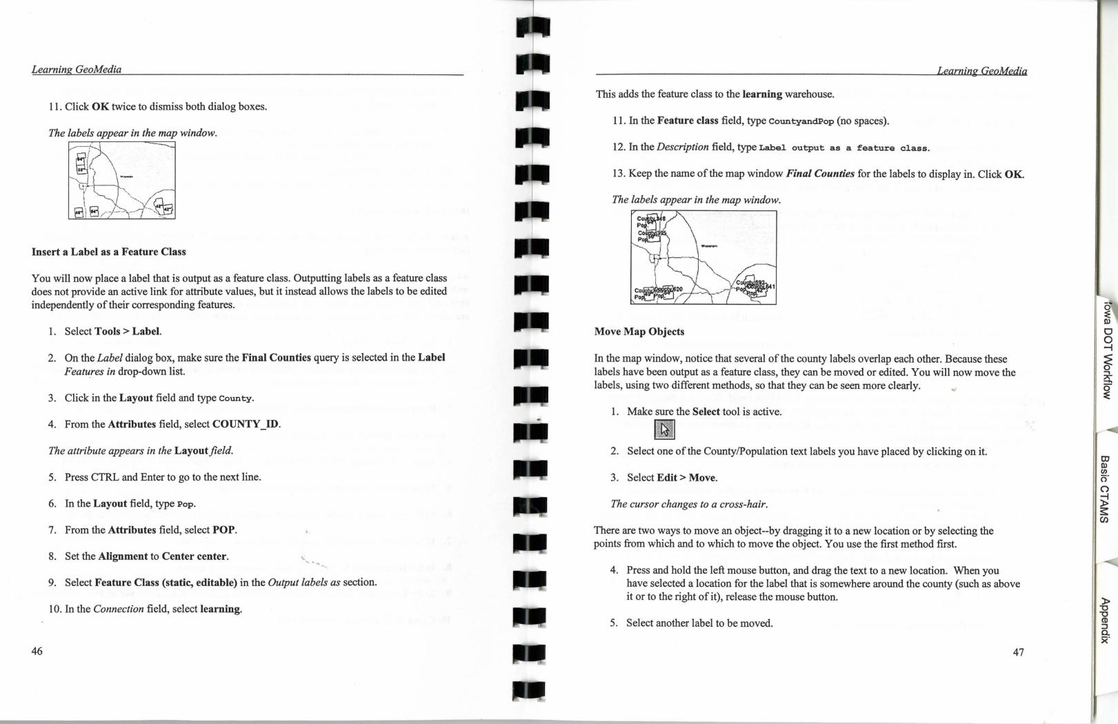
11. Click OK twice to dismiss both dialog boxes.

Insert a Label as a Feature Class

You will now place a label that is output as a feature class. Outputting labels as a feature class does not provide an active link for attribute values, but it instead allows the labels to be edited independently of their corresponding features.

46

1. Select Tools > Label.

2. On the Label dialo~ box, make sure the Final Counties query is selected in the Label Features in drop-down list.

3. Click in the Layout field and type County.

4. From the Attributes field, select COUNTY _ID.

The attribute appears in the Layout field.

5. Press CTRL and Enter to go to the next line.

6. In the Layout field, type Pop.

7. From the Attributes field, select POP.

8. Set the Alignment to Center center.

9. Select Feature Class (static, editable) in the Output labels as section.

10. In the Connection field, select learning.

Learning GeoMedia

This adds the feature class to the learning warehouse.

11. In the Feature class field, type CountyandPop (no spaces).

12. In the Description field, type Label output as a feature class.

13. Keep the name of the map window Final Counties for the labels to display in. Click OK.

The labels appear in the map window.

Move Map Objects

In the map window, notice that several of the county labels overlap each other. Because these labels have been output as a feature class, they can be moved or edited. You will now move the labels, using two different methods, so that they can be seen more clearly.

1. Make sure the Select tool is active.

2. Select one of the County/Population text labels you have placed by clicking on it.

3. Select Edit > Move.

The cursor changes to a cross-hair.

There are two ways to move an object--by dragging it to a new location or by selecting the points from which and to which to move the object. You use the first method first.

4. Press and hold the left mouse button, and drag the text to a new location. When you have selected a location for the label that is somewhere around the county (such as above it or to the right of it), release the mouse button.

5. Select another label to be moved.

47

Learning GeoMedia

You use the second method to move this object.

6. Select Edit > Move.

7. When the cursor changes to a cross-hair, click the pointfrom which you want to move the object.

8. Click the point to which you want to move the object.

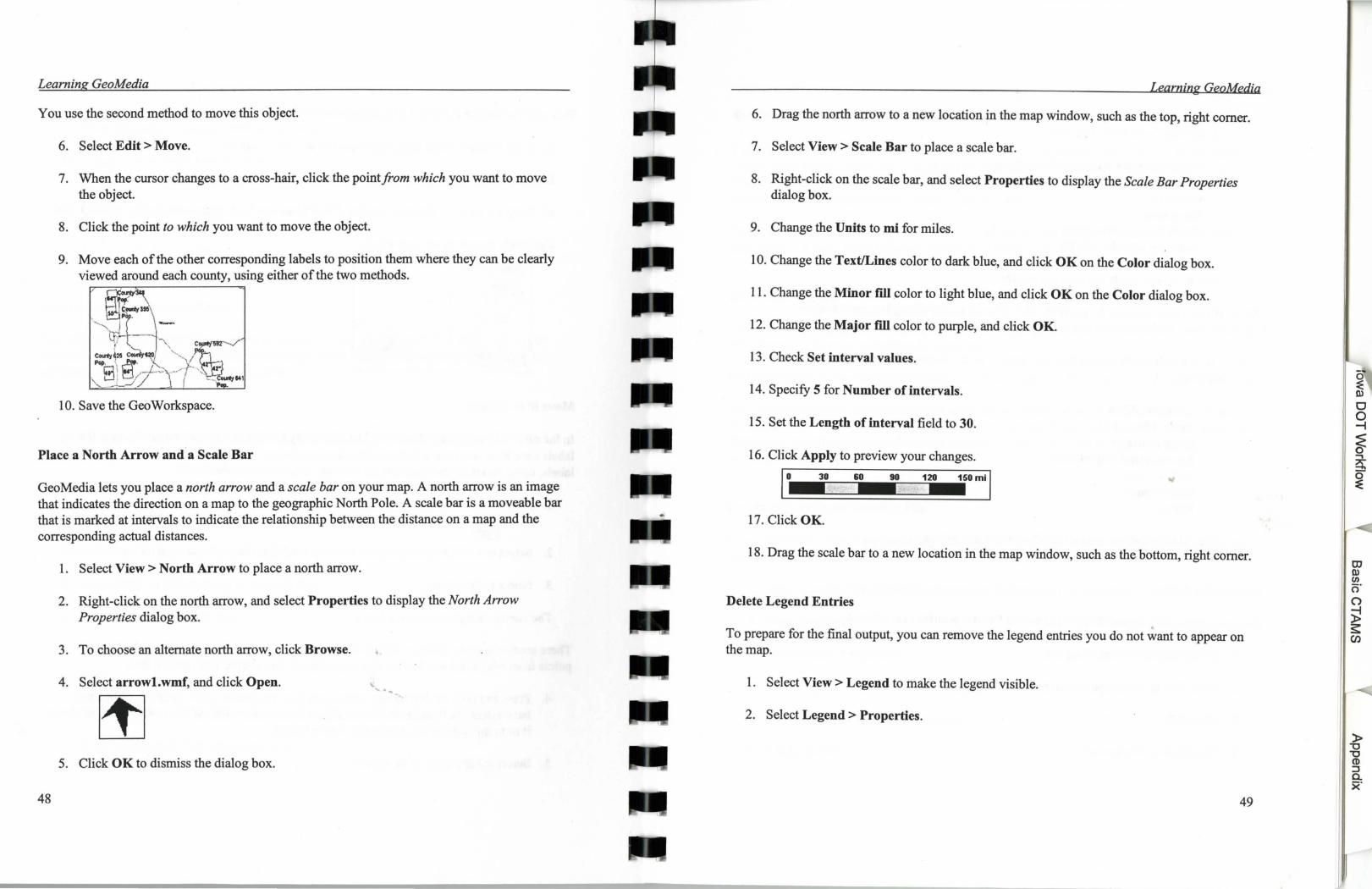
9. Move each of the other corresponding labels to position them where they can be clearly viewed around each county, using either of the two methods.

, t"j~ o·~~/ ~~25 ~h~) '··,··J .

t:l ] EJ __,-.L:.v• , ./f· ,~ ~l___.l/ r ---.~~ .. 1


Place a North Arrow and a Scale Bar

GeoMedia lets you place a north arrow and a scale bar on your map. A north arrow is an image that indicates the direction on a map to the geographic North Pole. A scale bar is a moveable bar that is marked at intervals to indicate the relationship between the distance on a map and the corresponding actual distances.

48

1. Select View> North Arrow to place a north arrow.

2. Right-click on the north arrow, and select Properties to display the North Arrow Properties dialog box.

3. To choose an alternate north arrow, click Browse.

4. Select arrowl.wmf, and click Open. . ..

5. Click OK to dismiss the dialog box.

Learning GeoMedia

6. Drag the north arrow to a new location in the map window, such as the top, right comer.

7. Select View> Scale Bar to place a scale bar.

8. Right-click on the scale bar, and select Properties to display the Scale Bar Properties dialog box.

9. Change the Units to mi for miles.

10. Change the Text/Lines color to dark blue, and click OK on the Color dialog box.

11. Change the Minor f"Ill color to light blue, and click OK on the Color dialog box.

12. Change the Major fill color to purple, and click OK.

13. Check Set interval values.

14. Specify 5 for Number of intervals.

15. Set the Length of interval field to 30.

16. Click Apply to preview your changes.

30 120 150mil

17. Click OK.

18. Drag the scale bar to a new location in the map window, such as the bottom, right comer.

Delete Legend Entries

To prepare for the final output, you can remove the legend entries you do not want to appear on the map.

1. Select View > Legend to make the legend visible.

2. Select Legend > Properties.

49

)> "0 "0 CD :J a. x·

Learning GeoMedia

3. Select the following legend entries, by clicking the row selector for the following entries, and holding down the CTRL key:

-Small Counties Around Major Cities -Cities -Counties -Interstates -States by snow/avetemp -States by ANNULSNOW

4. Click Delete to delete the selected entries.

NOTE: If you delete an entry by mistake, click Cancel on the dialog box andre-select Legend> Properties and follow the previous steps again.

5. Verify that the only entries that now appear on the Legend Properties dialog box are the following:

- CountyandPop - Annual Snowfall - Final Counties - ZoneAroundMajorCities -Major Cities - StateNames -States

6. Click OK to dismiss the Legend-Properties dialog box.

Rename the Legend

Now you rename the legend that is used by the Final Counties map window.

1. Select Legend > N arne Legend.

2. In the Name field, type LearningLegend2

3. Click OK.


50

Learning GeoMedia

+ Preparing the Results

You can plot your results using Imagineer™ Technical 2.0, which is delivered with GeoMedia. Using GeoMedia's custom map layout commands, Imagineer Technical 2.0 becomes a map presentation environment. In addition to the capabilities provided by GeoMedia's custom commands, all of Imagineer's capabilities are provided.

Before proceeding, make sure Imagineer is installed on your system. For maximum efficiency and speed, it is best to minimize but not dismiss GeoMedia. ·

Set Up for Plotting

To set up for plotting, you set the default printer on your system to be the one you want to use to plot the map and set up your sheet in Imagineer.

IMPORTANT: Set up the plotter before you start Imagineer. Ifimagineer is already open, close it.

The current system printer determines the resolution of the file that is created with the Frame Properties command. If you move the frame from one machine to another, you must update the links to the GeoMedia data so that the metafiles are re-created with the new resolution of the new default system printer.

Create an Imagineer Drawing File

You use the Imagineer template that is delivered with GeoMedia as a starting point for creating your final output.

1. Make sure that GeoMedia is running, but its window is minimized.

2. Start Imagineer.

3. Select Tools> Options.

4. Select the File Locations tab on the Options dialog box.

5. Select the User Templates file type.

6. Click Modify.

51

m m en c;· 0

~ s:: en

)> "0 "0 CD :J a. )("

Learning GeoMedia

7. Specify the location of the provided templates. By default, they are located in c: \Program Files\GeoMedia\Templates\lmagine.

8. Click OK on the dialog boxes.

9. Select File> New.

10. From the list of templates, select MapLayout-English.igt, make sure Document is selected, and click OK.

11. Select File > Sheet Setup.

12. On the Size and Scale tab, make sure Scale (1:1) is selected for the Drawing Scale.

13. Click OK to dismiss the Sheet Setup dialog box.

14. Select View > Fit.

The drawing sheet fits in the window.

1-,....~--.Jl!-1 -··· I w~VIICUICI L. - --'1 Plot Tttl•

Design the Layout of the Map

GeoMedia delivers three Map Layout tools that you can use in Imagineer: Design GeoMedia Layout (DesignLayout.exe), Frame Properties (EditFrameProp.exe), and Create Legend Graphics (LegendGraphics.exe). These can be found as a toolbar at the top of the Imagineer screen and look like this:

The Design GeoMedia Layout command lets you design a map layout, by placing frames on an Imagineer sheet. After placing the frames, you can use the Frame Properties command to populate them with a map view, scale bar, or north arrow from a GeoWorkspace.

52

Learning GeoMedia

This Map Layout template has three frames already placed on it. Two of the frames are to be used for map views, and one of the frames is to be used for a scale bar. You place a fourth frame, to be used for a north arrow.

1. From the Imagineer toolbar, select Design GeoMedia Layout.

[i] The cursor becomes a cross-hair, ready to place the first point of the frame.

2. Place the cursor anywhere in the area below the text, Map View Frame (Overview map).

+

Plot Tilla

3. Click the left mouse button to place the first point.

If you need to make a correction, you can discard a previously placed first point by right clicking, and then you can place another first point.

4. Diagonally from the first point, move the cursor to place a rectangle, similar to that shown below.

D

Plot Titla

5. When the rectangle is the size you want, click to place the second point of the frame.

53

Learning GeoMedia

6. With the Imagineer window active, press ESC to exit the Design GeoMedia Layout command.

It is always a good idea to save a document in case you have to come back to it later.

7. Select File > Save As ...

8. In the File name field, type learning to save the file as learning.igr.

9. Click Save.

Place GeoMedia Map Views in the Layout Frames

After designing the layout of your map, you edit each frame to link it to a GeoMedia GeoWorkspace object (a map view, scale bar, or north arrow).

54

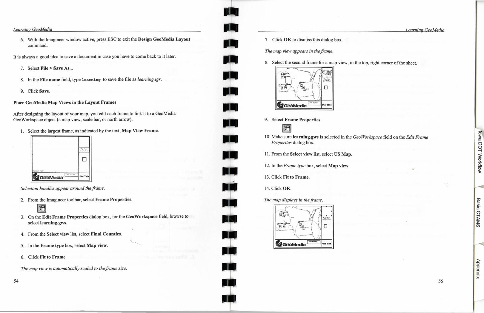
1. Select the largest frame, as indicated by the text, Map View Frame.

"ff ., •• •t--'.l.':': .. ~

0

1--~--.a:-1 - ·-· I w~v~ '-· -----'IPIOCTille

Selection handles appear around the frame.

2. From the Imagineer toolbar, select Frame Properties.

rg 3. On the Edit Frame Properties dialog box, for the GeoWorkspace field, browse to

select learning.gws.

4. From the Select view list, select Final Counties.

5. In the Frame type box, select Map view.

6. Click Fit to Frame.

The map view is automatically scaled to the frame size.

Learning GeoMedia


The map view appears in the frame.

8. Select the second frame for a map view, in the top, right comer of the sheet.

.--.. r·- ~ /~ ~ lvr:: "'""f' ~\- uf· ~ r· •rr.::::· . I ~ . ........- .. , ........ _

~)~~ -\ ~~-· { '·,~-. 0 ---~} \ ~ I

"\-·- . ) I , , / I

9. Select Frame Properties.

10. Make sure learning.gws is selected in the Geo Workspace field on the Edit Frame Properties dialog box.

11. From the Select view list, select US Map.

12. In the Frame type box, select Map view.

13. Click Fit to Frame.

14. Click OK.

The map displays in the frame.

,._~ i ..... ~ _,J •. " """ ·, -. . ..__, tv~(

· fir, 1;· · ~r··. _ rJ .. ~ -;:-......

) ·t ~ • J~!r:lt-~ !f:t""- /'. • ' I

~foL·~ .. , ~ { 't 0 ' 8 8 l '\ { -~· \ :1\

., --"'- ) ( ... ' -- '

''\.-----\ ) I , .... '- /L -

Cz I ""'""·~ Gee Media" I PIOITIII•

55

m ll) en (5" ()

~ s:: C/)

)> "0 "0 CD :J a. x·

Learning GeoMedia

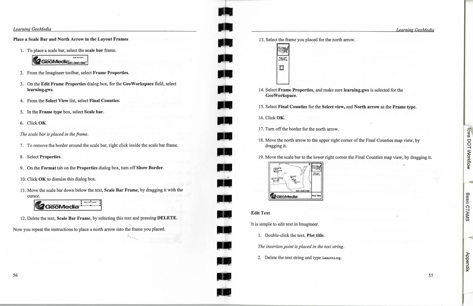
Place a Scale Bar and North Arrow in the Layout Frames

1. To place a scale bar, select the scale bar frame . .... ..,.... I ~'?(""'" ' • GeOMecllc:"". . . - -:

2. From the Imagineer toolbar, select Frame Properties.

3. On the Edit Frame Properties dialog box, for the GeoWorkspace field, select learning.gws.

4. From the Select View list, select Final Counties.

5. In the Frame type box, select Scale bar.

6. Click OK.

The scale bar is placed in the frame.

7. To remove the border around the scale bar, right click inside the scale bar frame.

8. Select Properties.

9. On the Format tab on the Properties dialog box, turn off Show Border.


11 . Move the scale bar down below the text, Scale Bar Frame, by dragging it with the cursor.

12. Delete the text, Scale Bar Frame, by selecting this text and pressing DELETE.

Now you repeat the instructions to place a north arrow into the frame you placed.

.......

56

Learning GeoMedia

14. Select Frame Properties, and make sure leaming.gws is selected for the Geo Workspace.

15. Select Final Counties for the Select view, and North arrow as the Frame type.

16. Click OK.

17. Tum off the border for the north arrow.

18. Move the north arrow to the upper right comer of the Final Counties map view, by dragging it.

19. Move the scale bar to the lower right comer the Final Counties map view, by dragging it.

Edit Text

It is simple to edit text in Imagineer.

1. Double-click the text, Plot title .

The insertion point is placed in the text string.

2. Delete the text string and type Learning.

57

m Ill en c=r ()

i! s: C/l

)> "0 "0 (l) :J a. )("

Learning GeoMedia

3. Replace the text string below the US map, Map View Frame, with Final Counties.

4. Replace the text string inside the parentheses, Overview map, with For ski. resort.

c , .... "-- ...... ·~· /~-. ----1 frf . ~. .

~~· ~~1 .. ' . { ·~~~~· \- .0 . ~

._ .. ~~· ~- { · , ~ ,) l i!i ''j / ... \ . ~--"-_ _,____ '1 1 ' I ' t ' "-4.___,-- j C

~- ---~-ta~bMedla· Lownlng

5. You can change the font or size of a text string by right-clicking the text, selecting Properties, and selecting the Paragraph tab.

Add a Legend

Create Legend Graphics converts the GeoMedia legend into graphic style keys and text that Imagineer can understand and edit.

Unlike map views, the legend you place in Imagineer is not linked to the original GeoMedia GeoWorkspace. To make changes to the new legend, you can either make change using Imagineer, or make changes using GeoMedia and then rerun Create Legend Graphics.

58

1. From the Imagineer toolbar, select Create Legend Graphics.

2. On the Create Legend Graphics dialog box, select learning.gws in the GeoWorkspace field.

3. Select the legend, LeamingLegend2, in the Legends field.

4. Select the option to Sort legend alphabetically.

5. Change the Font to Arial.

6. Click OK to close the dialog box.

Learning GeoMedia

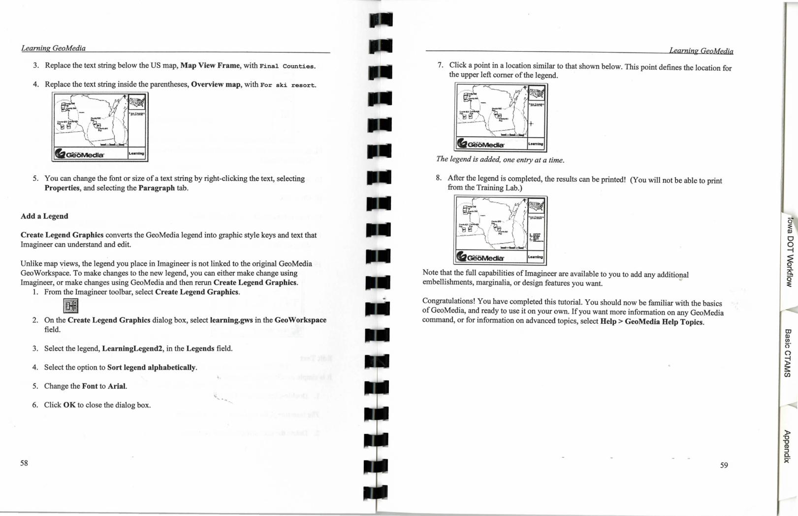
7. Click a point in a location similar to that shown below. This point defines the location for the upper left comer of the legend.

c .-..: -t' ....... ~ /-... ·----~vi . r~

~ 1' ,- t } ·~~· J .• / ., . t:"'f:t ~ / ''.) '. B ~)''j i ~-· I '\\ ~-- ·d ... \ ! +

'\~ /

.Gi!OMedia' Leem1n11

The legend is added, one entry at a time.

8. After the legend is completed, the results can be printed! (You will not be able to print from the Training Lab.)

£-- ~.;____ -t' ,.-··-·-·.. ---~ vi' . . ~rr·· ,.;._ 4Yf~ . -~ . ~. ..... (i' t ' $l':S.t-J.;lt•

·--·~K .~a: .. ; · . ~ ··aB' ".J i ' £l.-,. •. 1 '\'< ·-·---- ~ ~ \ i' t~

\..\..__---\ / .. =--\~\ ~-~'"'.

6Ge6Med1a· Lumln~

Note that the full capabilities oflmagineer are available to you to add any additional embellishments, marginalia, or design features you want.

Congratulations! You have completed this tutorial. You should now be familiar with the basics of GeoMedia, and ready to use it on your own. If you want more information on any GeoMedia command, or for information on advanced topics, select Help> GeoMedia Help Topics.

59

CD Ill en cr ()

~ s: Cll

)> "0 "0 CD :J a. x·

60

Iowa DOT GIS Workflow

Using data produced by the Iowa DOT and the Iowa DNR, you will learn how to use data from different data warehouses to create a map display of features of interest. Rather than displaying all features from the warehouses on the map, you will learn how to limit the data displayed to only that data of interest to you. Specifically, you will learn how to:

• Define and apply a filter to a warehouse connection. • Formulate and perform a query to retrieve and display particular feature data. • Create a buffer zone to display feature data that shares a defined physical proximity with

another feature. • Create a thematic map to illustrate the occurrence of data of interest. • View data related to specific features in a data window.

Like the GeoMedia tutorial, these exercises build upon each other to demonstrate how to combine, search, and display data from multiple, large data sources to arrive at very specific geographic information. In this exercise, we will be identifying. primary roads with a certain surface type and AADT, population density of a county, and wetlands or rivers that cross into a new road design. The combination of this data will lead to answers about where certain features exist in the State of Iowa.

Getting Started

Create a new Geo Workspace.

File>>New GeoWorkspace >Document >OK

Be sure to save the workspace and give it a name such as ACCRoads.

You will also need to set the coordinate system for the Geo Workspace.

View>>Geo Workspace Coordinate System >Projection Space tab>>select Universal Transverse Mercator >Geographic Space tab>>select North American 1927 >OK

File>>Save GeoWorkspace

61

)> "0 "0 CD :J a. x·


+ Lab I - Iowa DOT Data

In the first part of this workflow, you will be trying to identify primary roads in the state that may be in need of repair or replacement. To do this, several things will be looked at such as surface type, AADT, and ACC Ratings. This data is found on the Iowa DOT base record which has been converted to Access for this exercise.

Connecting to the Data

The Iowa DOT road data is in an Access database on the CD.

Warehouse>>New Connection >Browse the CD for d:\TrainingCD\Idot\Road2.mdb >Click the Read Only box on the Browse screen

Don't forget to name the connection (/dot data) and open it as Read Only.

Displaying Features

You will want to display the feature: county borders.

Legend>>Add Feature Class >From Connections select (/dot Data) >From Feature Classes select border

Performing a Query on a Warehouse

To refine your data display for the specific information that you are interested in, you can perform a query to search the data for particular feature attributes such as a certain pavement type or a particular level of traffic. For this exercise, instead of adding all the primary roads, you will query the road data to identify portions of the primary highway with a certain surface type( asphalt, 60-69) and a certain traffic level (2000).

Tools>>New Query ..... • ... >Select Features In: choose (/dot data}>>primary _road >Select the Filter button. Enter this filter: SURF TYPE >= 60 AND

SURF_ TYPE <= 69 AND AADT > 2000 >OK Name: Don't forget to enter a name for the query (ACCRoads)

62

Iowa DOT GIS Work{low

Description: Optional >OK

-------- -

The query will be performed, added to the legend, and displayed in the Map Window. This may take a couple minutes.

Creating a Thematic Map

You can create a thematic map to better display the results of your work. In this case, we will create a thematic map of the ACC Roads based on their ACC rating.

Legend>>Add Thematic Feature Class: >Queries> select (ACCRoads) Available Attributes: select acc_rating >Unique>> >Defme (this may take a few minutes)

Change Label: to Descriptions Style: fair change to yellow, weight=3.0

good change to green, weight=3.0 poor change to red, weight=3.0

>OK to dismiss Define window >OK to dismiss Thematic Map window

This will display the ace _rating by color on the roads from the previous query. Red segments could be considered areas for further investigation into road improvement.

Since the thematic map will cover up the query display, you can turn it off.

Right click on the legend entry (ACCRoads). >select Display Off

Right click on the legend entry (ACCRoads). >select Hide Legend Entry

ACCRoads was removed from the legend display.

Save the Workspace

File>>Save Geo Workspace

63

)> "0 "0 CD :J a. )("


+ Lab II · Iowa DNR Data

In this lab, we are going to concentrate on one county (Clay) that showed red segments from the thematic map in the first lab of this workflow. We will try to find out if any of the red segments fall within areas of moderately-high population.

Opening a New Map Window

We want to save the thematic map that was created in Lab I and focus in on a smaller area so '

we want to open a new map window.

Window>>New Map Window >Window Name: (Clay) >OK

New Query

We need to find Clay County by doing a query on the border feature class.

Tools>> New Query >Select Features In: select (/dot Data)>>border >Filter: CO _NAME= 'Clay'

>OK >Name: (Clay County) >OK

Connecting to DNR Data

The Iowa DNR data is in an ArcView database on the CD.

Warehouse>>New Connection >Browse the CD for d:\TrainingCD\DNR\Clay

Don't forget to name the connection( ClayDNR).

Defining a Connection Filter

To limit the data you see to a particular area, such as Clay County, you can apply a connection · filter to one or more warehouse connections.

64


To define a connection filter:

Warehouse>>Defme Connection Filter Filter Name: type Clay Spatial Operator: >Inside Placement Options: >Create a new filter by selecting an area geometry >Defme

>Click once inside the Clay County border to highlight it >Double click inside border to confirm.

>Select Close when Define Connection Filter dialog box reappears.

To apply the connection filter:

Warehouse>>Edit Connection >select the Connection Filter column in the ( ClayDNR) row

>Select Clay County >Connection Filter column (/dot Data)

>Select Clay County

The results of the connection filter will only be displayed on actions taken from this point forward (the filter is not visibly displayed).

Save the Workspace


Creating a Thematic Map

Now, we will create a thematic map of population based on the census block data provided by the Iowa DNR.

Legend>>Add Thematic Feature Class:> (ClayDNR) >select cen90_clay Available Attributes: select TOTALPOP >Range>> >Defme (this may take a few seconds)

Range technique: select Equal Count Number of Ranges: select 5 >Hit the Color Selection button to choose a color scheme. (Green looks good)

65

OJ fl) en ()" ()

~ s: C/l


Label: select Description Optional: Change all the decimals to the next highest whole number. >OK to dismiss Define window

>OK to dismiss Thematic Map window

This will display the total population by color in Clay County.

Performing a Spatial Query

A spatial query is used to find features of interest that fall geographi:ally close.to .another . feature. You will use this to see if any of the roads with poor ace ratmgs are w1thin a certam distance of the moderately high populated areas.

Tools>>New Query Select features in: select Queries>(A CCRoads)

Filter: type acc_rating ='poor' >Hit the Spatial button

That: select are within a distance of Distance: type 10 Units: select mi

Select Features in: select (ClayDNR)>cen90_clay Filter: type TOTALPOP > 150

Name: name the query (In_ Need) >OK

The results of the spatial query will appear in your map window. If you cannot see it, you may want change the style of the feature. To do this, double-click on the Legend entry, and change

the color and weight of the line.

Save the Workspace


66


+ Lab Ill- Accident Data

Now that we have located potential roads in need around moderately high populated areas, we can take a look at accident data to see if the road may be the cause of serious injury or fatal accidents.

Connecting to Accident Data

The accident data is in two different Access databases on the CD. One contains the point feature of the accident and the other contains the information about the accident.

Warehouse>>New Connection >Browse the CD for d:\TrainingCD\Idot\ClayCrashLoc.mdb >Click the Read Only box on the Browse screen

Don't forget to name the connection(CrashLocations).

Warehouse>>N ew Connection >Browse the CD for d:\TrainingCD\Idot\ClayCrashData.mdb >Click the Read Only box on the Browse screen

Don't forget to name the connection(CrashData).

Joining Features to Attributes without Geometry

Data in crashdata does not contain a map location, which means it can not be shown in the map window by using Add Feature Class. Since the accident location file and the accident data file both contain the case number of the accident, we are able the join the table that contains a map location (crashlocations) and the table that does not contain a location (crashdata).

Tools>>Join Left side of Join: select CrashLocations>>CrashLocations Right side of Join: select CrashData>>CrashData Available Attributes: select CASE NUM from both sides >Click the down arrow Type of Join: select Inner Query N arne: type Accidents >Click the Display join in Map Window box

Map Window Name: select Clay Style: you can change if you like

67

)> 'U 'U m :J c. x·


>OK

>Click the Display join in Data Window box Data Window Name: type Accidents

Move the Data and Map Windows around so that you can them both.

>Double click on an accident point and watch that it highlights in the data window. The information box also appears with all of the data in it.

>Close

You can now close the Data Window (Accidents) .

>Select the Data Window (Accidents) by clicking on it once. >Click on the X in the upper, right hand comer of the Data Window

Performing a Spatial Query

Before performing the query, in order to see the results of it better, the existing accident display needs to be turned off.

>Click on the Accident entry in the Legend. >Right-click on the mouse

>select Display Off

Now we can do a spatial query to bring in all fatal accidents that have occured along the sections of road found in the In_Need query.

Tools>>New Query Select Features In: select Queries>> Accidents >Spatial button That: select touch Features In: select Queries>>/n Need Name: type Accidents Touching Road >OK

....

Only one accident appears and you know from looking at the join data that there appeared to be more along the road. This is because of accuracy differences in the two data sets and the actual location of the accident might not be on the road. Also,-ifyou would want to include accidents on intersections along the route, they might be located on the other leg of the intersection that was not queried on.

68


We will do another query that more accurately reflects that accidents along the route by looking for accidents that occur within 50 feet of the road.

Tools>>New Query Select Features In: select Queries>> Accidents >Spatial button That: select are within a distance of

Distance: type SO Units: select ft

Features In: select Queries>>ln_Need Name: type Accidents by Road >OK

You may have to change the color to see the new query better. Double-click on the Legend entry to change the style.

The results of this query find more accidents than the previous one.

New Query

Now, we can_ do another query to find all of the fatal accidents of the ones that were within 50 feet of the road.

Tools>>New Query Select Features In: select Queries>> Accidents By Road >Filter button

Type in G_SEV = '1' (stands for fatal accident) >OK

Name: type Fatal Accidents >OK

Three fatal accidents were found along the In Need section of road.

Save the Workspace


69

)> "0 "0 (t) ::l a. x·


+ Lab IV -Data Window Features

The data window is helpful when you want to actually see the values returned by a query, or all of the information associated with a feature class. From the Data Window, you can also hide columns, promote rows to the top, and copy information to another spreadsheet such as Excel or Lotus. First, to open a Data Window:

Window>> New Data Window •.• Name: type In_Need >Choose Queries>>(/n_Need) >OK

To hide some of the columns:

>Click on the column name (Key _Id) >Right-click on the mouse

>select Hide Column

Another way to hide columns:

Data>>Show Columns >Leave only the following checked:

CO AADT ST RTE SURF TYPE NBS MPH_LIMIT STREET acc_rating YR CNT

>OK

Let's say that we are only interested in the sections around the city of Spencer. To find these without a query:

Window>>Cascade >Move the windows so that you can see the data window and the Clay County

window. · '-

>In Clay County window, right-click on census thematic map >select Locatable (This is so you will not be able to select this feature when you

drag the arrow across the map window.) >With the pointer in the Clay County window, click and drag a fence around the city

and include possible roads in need. (The sections will highlight in the data window.)

70


To copy the data to a spreadsheet:

>Switch to the Data window (click on it) >Data>>Promote Rows (This moves the rows to the top of the screen). >Go to the bottom highlighted row and click in the frrst cell in the frrst column and

drag up and across to re-highlight all of the rows selected by the fence. >Right-click on the highlighted part >select Copy

>Open Excel (without closing GeoMedia) >Right click on Excel or Lotus spreadsheet >select Paste

Now the selected sections have been put into an Excel spreadsheet and can be further manipulated into different formats.

Save the Workspace


71

' m ID en o· 0

~ s:: en

)> "0 "0 ro :J a. x·


+ Lab V - Design Files

An area for improvement has been located and a design of a by-pass around the city of Spencer has been started. Before work can be performed, environmental issues need to be investigated. By bringing in a design file and adding other data to the window, you can see what the new alignment of the road will affect in the field.

Opening a New Map Window

We want to save the what is in the previous window and focus on yet a smaller area, so we want to open a new map window.

Window>>New Map Window >Window Name: (EIS) >OK

Adding a Query to the Map Window

To make sure that are design file is brought into the correct area, we will need to query for Clay · County.

Legend>>Add Query >Select Clay County >OK

Connecting to a Design (CAD) File

The design file is read through a CAD schema definition(* .csd) file on the CD. It has already been created for this exercise, but normally you will have to create one for each design file you wish to bring into GeoMedia.

Warehouse>>New Connection >Browse the CD for d:\TrainingCD\cad\us71'propl.csd

Don't forget to name the connection(Design).

72


Displaying Features

The * .csd file created features out of the entities found on specific levels, so these features need to be added to the map window before they can be viewed.

Legend>>Add Feature Class >From Connections select (Design) >From Feature Classes select New Road

Save the Workspace


Removing Legend Entries

Since it appears that the design appears in the right location, you can take the Clay County border off of your map window and zoom in closer on the design on the new road.

>Click on the legend entry Clay County >Hit the Delete key

Message box: Delete legend Entries? >OK

The Clay County border is removed from the legend and the map window.

To see the new road design better:

View>> Fit All

Creating a Buffer around Features

To identify features of interest that occur near primary features, you can create a buffer zone around a feature class to limit the display to those features only within a defined proximity to the primary fea~e. For this exercise, you will create a buffer zone around a the new design of the highway.

73


To create a buffer zone, we must first create a new warehouse with a read/write connection.

Warehouse>>New Warehouse >select Document >OK File Name: type (Spencer) Save As Type: select Access >Save

Now we can create a buffer zone.

Insert>>Buffer Zone Buffer Zone Around: select (Design)>NewRoad Warehouse: select (Spencer) Feature Class: type Limits Constant Distance: type 150 >select ft Buffer Type: select Line>round >Merged >OK

Connecting to Statewide DNR Data

The Iowa DNR data is in an Arc View database on the CD.

Warehouse>>New Connection >Browse the CD for d:\TrainingCD\DNR\Statewide

Don't forget to name the connection(StatewideDNR).

Querying a Buffer Zone

After creating the buffer zone, we can query the data for particular features to see if they occur within the buffer zone. We will use the Statewide DNR data to query for underground storage

tanks within the buffer zone of 150 feet from the new desigB,__ ... Tools>>New Query

>Select Features In: >(StatewideDNR)>storage _tanks _regulated_ underground

>Spatial That: select are entirely contained by

74


Features In: select (Spencer)> select Limits Name: Don't forget to enter a name such as (UST near Design) >OK

The query will be performed, added to the legend, and displayed.

To see the data connected to the features within the buffered query, we can open a new data window with those data in it:

Window>>New Data Window >Select Queries> select (USTnearDesign) >OK

Or to see just the information associated with one site:

>Double-click on the point associated with the site that you want information about

Changing the Point Symbol

It is possible to change the point symbol to another kind of symbol. We will change the UST sites in the project area to a different symbol such as a star.

>Double-click on the symbol for UST near Design in the Legend. Type: select Symbol Symbol: scroll through the list until you find a symbol you like, Star for example.

If you highlight it in the list, the symbol will display in the sample box. >OK

Save the Workspace


Defining a Buffer as a Connection Filter

Instead of doing a spatial query to find all the features within a buffer zone, you can define a b~ffer zone as a filter, turn the filter on, and add the features through the legend to your map wmdow.

75

OJ fl) C/)

c=r (')

i! s: en

)> "'0 "'0 (I) ::J a. x·


Warehouse>>Defme Connection Filter Filter name: type (DesignBuffer) Spatial Operator: select Overlap Placement Options: select Create a new filter by selecting an area geometry >Defme

>Click inside the buffer >Double-click to accept the buffer as your filter

>Close

To tum the filter on:

Warehouse>>Edit Connection >select the Connection Filter column in the ( ClayDNR) row >select (DesignBuffer)

>Close

Displaying Features

Now, any features that you add to the map window from the (CiayDNR) will appear within the filter that we created from the design buffer zone. We will add rivers and wetlands to see if there are areas of concern along our new road design.

Legend>>Add Feature Class Connection: select ( C/ayDNR) >select rivers_ clay >OK

To use the wetlands data, you will need to query the feature class for all the areas that are wetlands:

Tools>>New Query Select Features In: select ( C/ayDNR) >>wetld _clay Filter: type DESCl <> 'U' (<>means not equal to) Name: type (Wetlands) >OK (This may take a minute.) ...

To make the wetlands easier to distinguish, we will do a thematic map:

Legend>>Add Thematic Feature Class: select Queries>>(Wetlands)

76


Available Attributes: select DESCl >Unique>> >Defme

Label: select Descriptions >Hit the Color button until you find colors you like >OK

>OK

Save the Workspace


77

)> "0 "0 (I) ::l 0. x·


+ Lab VI - Imagery

Imagery can be brought into GeoMedia. In this lab, we will bring in a scaned aerial photograph that has been registered through IRAS C and a USGS Digital Raster Graghic (DRG). The DRG is a digital raster image of a USGS paper map and is useful for data collection or as a base overlay in GIS.

To insert an image, there has to be an Access warehouse open with a read/write connection. We already have a read/write warehouse open (Spencer) that we used to create the buffer zone.

Inserting an Image - Aerial Photograph

Insert>>Image Image Name: select Browse

Browse to d:\TrainingCD\Images\21071006161.cot Pop-up message box File Marked as Read Only: select OK

Warehouse: select Spencer Placement Mode: select By Header Coordinate System Information File: select Browse

Browse to d:\TrainingCD\CAD\IowaNorthStatePlane.dgn >OK

To see the features that are now under the picture:

Click and drag the legend entry to the bottom of the legend list.

To see the photograph better:

View>>Zoom>>ln >Click and drag a box around the picture -OR->Click once on the picture and repeat until you are close enough to see the photo.

>ESC to return to the arrow cursor.

To see the whole design area again: ....

View>> Fit All

78

Iowa DOT GIS Work[low

Inserting an Image - DRG

Insert>>Image Image Name: select Browse

Files of Type: select TIFF (* .tif) Browse to d:\TrainingCD\Images\043095b2.tif Pop-up message box File Marked as Read Only: select OK

Warehouse: select Spencer Placement Mode: select Georeferenced >OK

To see the features that are now under the picture:

>Click and drag the legend entry to the bottom of the legend list.

To see the DRG better:

View>>Zoom>>ln >Click and drag a box around the area you wish to zoom in on -OR->Click once on the picture and repeat until you are close enough to see the photo.

>ESC to return to the arrow cursor.

With all the windows you created, you can use Imagineer to create a layout of the information that you have found.

79

)> "0 "0 CD :J a. x·

\.. ....... --

80

m ID en cr ()

~ s:: (JJ

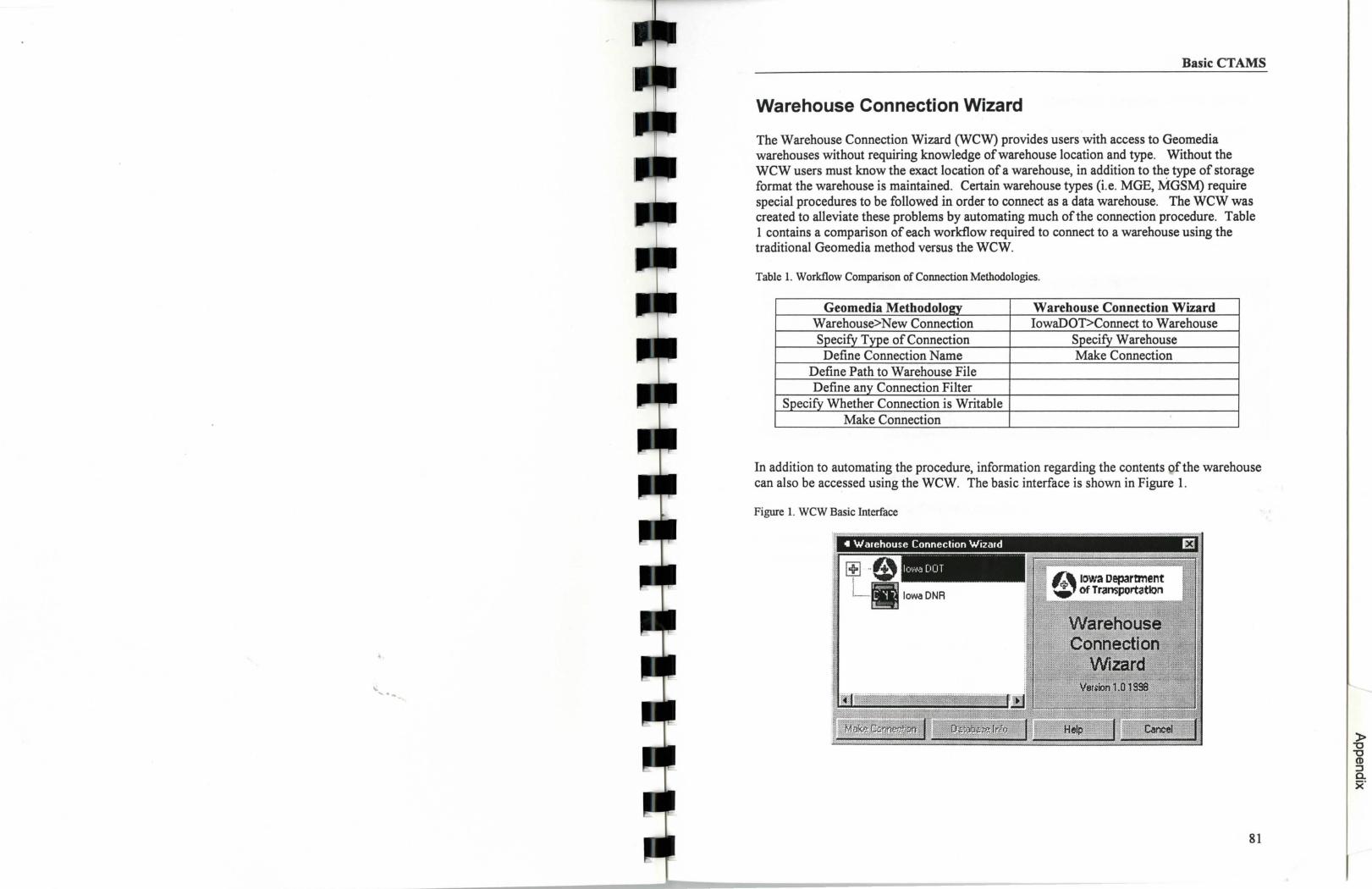
BasicCTAMS

Warehouse Connection Wizard

The Warehouse Connection Wizard (WCW) provides users with access to Geomedia warehouses without requiring knowledge of warehouse location and type. Without the WCW users must know the exact location of a warehouse, in addition to the type of storage format the warehouse is maintained. Certain warehouse types (i.e. MGE, MGSM) require special procedures to be followed in order to connect as a data warehouse. The WCW was created to alleviate these problems by automating much of the connection procedure. Table 1 contains a comparison of each workflow required to connect to a warehouse using the traditional Geomedia method versus the WCW.

Table 1. Workflow Comparison of Connection Methodologies.

Geomedia Methodolo Warehouse Connection Wizard W arehouse>N ew Connection IowaDOT>Connect to Warehouse

Define Connection Name Define Path to Warehouse File

Make Connection

In addition to automating the procedure, information regarding the contents of the warehouse can also be accessed using the WCW. The basic interface is shown in Figure 1.

Figure 1. WCW Basic Interface

81

)> "0 "0 <D :J a. x·

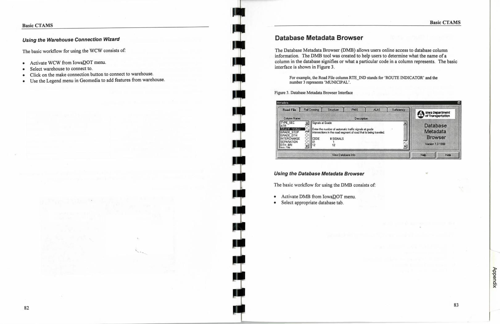
BasicCTAMS

Using the Warehouse Connection Wizard

The basic workflow for using the WCW consists of:

• Activate WCW from IowaDOT menu. • Select warehouse to connect to. • Click on the make connection button to connect to warehouse. • Use the Legend menu in Geomedia to add features from warehouse.

~ .......

82

BasicCTAMS

Database Metadata Browser

The Database Metadata Browser (DMB) allows users online access to database column information. The DMB tool was created to help users to determine what the name of a column in the database signifies or what a particular code in a column represents. The basic interface is shown in Figure 3.

For example, the Road File column RTE IND stands for 'ROUTE INDICATOR' and the number 3 represents 'MUNICIPAL'. -

Figure 3. Database Metadata Browser Interface

Using the Database Metadata Browser

The basic workflow for using the DMB consists of:

• Activate DMB from IowaDOT menu. • Select appropriate database tab.

83

)> "'0 "'0 CD :J a. x·

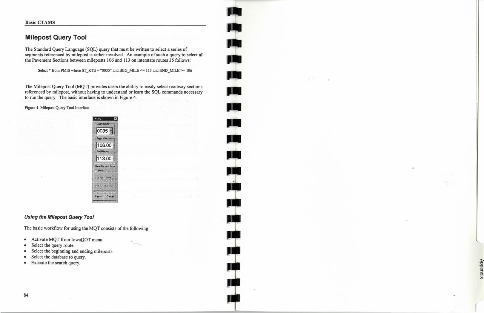
Basic CTAMS

Milepost Query Tool

The Standard Query Language (SQL) query that must be written to select a series of segments referenced by milepost is rather involved. An example of such a query to select all the Pavement Sections between mileposts 106 and 113 on interstate routes 35 follows:

Select* from PMIS where ST_RTE = "0035" andBEG_MILE <= 113 andEND_MILE>= 106

The Milepost Query Tool {MQT) provides users the ability to easily select roadway sections referenced by milepost, without having to understand or learn the SQL commands necessary to run the query. The basic interface is shown in Figure 4.

Figure 4. Milepost Query Tool Interface

Using the Milepost Query Tool

The basic workflow for using the MQT consists of the following:

• Activate MQT from IowaDOT menu. • Select the query route.

. .. • Select the beginning and ending mileposts. • Select the database to query. • Execute the search query.

84

II

)> "0 "0

CD :J a. x·

·~

..

ApPendix A

Hypertext Links

Hypertext is a link to an external file. When the link is executed (double-clicked), the application associated with the file is invoked, and the file is opened or played by clicking the hypertext cell in the data window. To create a hypertext link, a new feature class must be created in a read/write warehouse connection, and must be added to the Map Window in the GeoWorkspace. Then a hypertext link must be added to the feature table so that it will show in the data window when the feature is selected.

Open a read/write warehouse connection (Only do this if a read/write connection for your project is not already open.)

Select Warehouse>>New Warehouse In the New window, select normal.mdb and make sure that document is selected.

Click OK.

In the New Warehouse window, type a name to save the warehouse as, and click OK.

Create a New Feature Class

Select Warehouse>>Feature Class Defmition Highlight the warehouse that was just created (or highlight your existing read/write

connection), and then select New.

The New-FeatureC/assl window opens on the General tab. In the Name: category, type in your feature name. In the Description: category, type in a description (optional). In the Geometry Type: category, chose the type of geometry that you want to

represent the new feature.

Now, select the Attribute tab at the top of the New-FeatureC/assl window.

First Row Select on the cell in the first row under the Key column. (A gold key should

appear). Select the cell in the first row under the Name column and enter ID. Select the cell in the first row under the Datatype column, and from the pull

down window select Autonumber.

85

Appendix A

86

Select the cell in the first row under the Description column, and enter a description of the ID field if desired. (This field gives each feature in the new feature class a unique ID to locate the feature in the Data Window.)

Second Row Select the cell in the second row under the Name column and enter Type. Select the cell in the second row under the Datatype column, and from the pull-

down window select Character. Then change the Length: category to 20. Select the cell in the second row under the Description column, and enter a

description of the Type field if desired. (This field can be used to explain what the point (feature) in the GeoWorkspace is representing such as a photograph or a certain type of sign-variable message.)

Third Row and so on (You can continue to add rows until all the data that you want to enter about that certain feature is complete.)

Select the cell in the row under the Name column and enter a name category for the data field.

Select the cell in the row under the Datatype column, and from the pull-down window select one of the following:

Character - if you want to enter an alphabetic type description. Make sure that you change the Length field to reflect the length of the description that you want to enter.

Number - if you want to enter a numerical type description. Make sure that you change the Format, Size, and Decimal Places fields to reflect the data that you want to enter.

Currency - if you want to enter a dollar amount type description. Make sure you change the Format and Decimal Places fields to reflect the data that you want to enter.

Date - if you want to enter a date as a description. Make sure you change the Format field.

Boolean - if you want to enter a boolean type description (yes/no, on/off, etc.). Make sure to change the Wording: field.

Select the cell in the row under the Description column, and enter a description of the field if desired.

Last Row (Hypertext row) Select the cell in the last row under the Name column and enter a name for the

hypertext link (i.e. image for photograph files).

Appendix A

Select the cell in the last row under the Datatype column, and from the pulldown window select Character. Then change the Length: category to 50 or longer depending on the length of the path to the file. Make sure that the box beside Hypertext at the bottom of the window is checked.

Select the cell in the last row under the Description column, and enter a description of the field if desired.

Select OK, and then click Close on the Feature Class Definition window.

Insert a Feature in the Map Window

To be able to view the added feature once you have added it, you will need to add the new feature class to the legend: Legend>> Add Feature Class, then chose the read/write connection name and the name of the new feature class that you just created.

Zoom to the area that you wish to place the new feature by using the Zoom Tools.

Select Insert>>Feature. On the tool bar that is added at the top of the screen, click the drop-down menu

arrow and select the read/write connection and name of the feature class that was just created. (The cursor will turn to cross-hairs.)

Click once on the spot that you wish to place the new feature, and select OK on the Properties window that pops-up. Repeat as many times as needed.

Insert Feature Attributes (Including Hypertext)

Open a Data Window for the new feature class. Select Window>>New Data Window. In the New Data Window window, select the read/write connection name and the

new feature class name. Click OK.

Enter the attributes and hypertext links in the Data Window. Select the type cell of the feature and enter the corresponding type. ~elect any other field cell and enter the corresponding data.

Right click in the hypertext cell. In the list, choose Hypertext>>Insert. In the Insert Hypertext window, find the name of the file that you want linked to

that specific feature (ID number) in the new feature class, and select OK.

87

Appendix A

(A path name should appear underlined and blue in the hypertext column cell.) To have the Data Window accept the path name, make sure that you click in a

different cell before closing the window.

Once all the features in the new feature class have all the data and hypertext links added to the data window, close the Data Window 1.

Hit ESC or click the arrow button to get out of the Insert feature mode.

Opening the Hypertext Link

Double-click on the new feature in the Map Window.

Then, click on the hypertext link (underlined and in blue) and the application with the appropriate file is launched.

Another way is to click once on the feature, and then right click. Choose Select Set Properties and click once on the hypertext link to launch the file.

·~

88

Appendix A

Displaying CAD Files in GeoMedia

The * .csd file is used to bring Micro station or AutoCAD design files into GeoMedia for viewing. The * .csd file defines the features of the CAD design file by level, color, style, type, weight, etc.

In order to define the features that are in the design file, a leveling chart or knowledge of which features reside on which levels is needed.

When displaying CAD drawings in GeoMedia, a warehouse connection is established similar to the way a warehouse is necessary for MGE, Arc View or Access. One of the necessary parameters when connecting to a CAD warehouse is a CSD file. These instructions step through the process of creating that file. ·

Creating a *.csd File

In the Start Menu>>Programs>>GeoMedia, chose the CAD Server Setup Utility.

In the CAD Server Schema box under Create a new CAD Server Schema using, choose Microstation and click OK.

It will open the CAD Server Definition- Microstation Template with the Files tab selected.

In the Directories section, chose New.

Select the directory where the design file(s) is( are) located. You should see the design files in that directory appear under the Map files in directory: Available Maps: section.

Highlight the design files in the Available Maps: section that you want to bring up in GeoMedia and then click the ">" arrow button.

Now, in the Directories section, chose New to find the directory with the Coordinate System File (This will either be IowaNorthStatePlane.dgn, or IowaSouthStatePlane.dgn).

Select the directory where the coordinate system file(s) is( are) located. Highlight the directory that contained the coordinate system file(s) under the

Directories section (the coordinate system files should appear in the Coordinate System files in selected directory, Available Coordinate System files: section).

89

Appendix A

Highlight the Coordinate System file in the Available Coordinate System files: section

and click the ">" arrow button.

At the top of the CAD Server Definition window, click on the Feature Defmition tab.

In the Feature Class section, chose New. This is where a leveling chart is needed.

90

Enter a unique name for the feature that you are defining in the first blank. This must not contain any characters other than letters, numbers, and underbars.

Specify the file defining the coordinate system by clicking on the down arrow and selecting the same file as you did in the Available Coordinate Systems files(IowaN orthStatePlane.dgn or IowaSouthS tatePlane.dgn).

Click Next.

In the Feature Attributes section, under Available attributes, highlight at least one of the following: (Use the graphic type if a backdrop of the design file is wanted and use the spatial type if you want to query or buffer the design file.)

GraphicAlly

GraphicArea GraphicLine GraphicPoint GraphicText

SpatialAny

SpatialArea

SpatialLine

SpatialPoint

if there is more than one type of element (point, line, polygon) on the level of the feature class you are defining or you do not know what type of element is on the level if the elements on the level are polygons if the elements on the level are linework if the elements on the level are point coverages if the elements on the level are text (this is the only option that will

bring in text)

if there is more than one type of element on the level of the feature class you are defining and you want to be able to query or buffer

based on the feature you are defining if the elements on the level are polygons and you want to query or

buffer by the defined feature if the elements on the level. are linework and you want to query or

buffer by them if the elements on the level are point coverages and you want to

query or buffer by them

and then click the ">" arrow button.

Appendix A

In the Primary geometry section, make sure that there is a checkmark beside the graphic/spatial option that you want to be considered the default geometry (especially if you chose more than one option).

Click Next.

Under Feature Definition Attributes, Available attributes: highlight at least one of the following (this defines what elements are considered part of the feature that you are defining):

Level Puts all elements that meet the level criteria into this feature class Color Puts all elements with a certain color into this feature class (should

be used with the level attribute). Style Puts all elements with a certain style into this feature class (should

be used with the level attribute). Type Puts all elements with a certain type into this feature class (should

be used with the level attribute). Weight Puts all elements with a certain weight into this feature class

(should be used with the level attribute).

and then click the ">" arrow button.

In the Enter feature definition attribute values dialog box, each feature that was picked in the previous step shows up in the Graphic attributes column. Position your cursor in the Value column and click on the left mouse button. When the cursor appears, enter the values associated with the element located in the Graphic Attribute column of the same row. For example, in the level row, enter the level number in the value column that the feature in question is located on.

Click Next.

In the Maps, Available maps: section, highlight all the maps that either contain this feature or that you want associated with this * .csd file, and then click the ">" arrow button.

Click Finish.

Repeat these steps for any other feature that you would like displayed in GeoMedia. It is possible to put elements from more than one level in the feature class that is being

91

Appendix A

92

defined. To do this, instead of entering one number in the value field, enter as many as you want by listing like this: 1-5 or 1, 2, 3, 4, 5 or 1-4, 7, 8, etc.

When you are finished defining all the features, click the X in the top right comer or go to File>>Exit.

When asked to save file, select yes, and save the file to a directory (preferably were the project is located).

Connecting to a CAD warehouse

Select Warehouse>>New Connection

In the Connection Type box, select CAD and then click on Next

Type in a name for your CAD connection Browse for the .csd you just created Type in a description for the connection (optional) Click on Next

Select Access all features in the warehouse Click on Next

Select Let the wizard open the connection as read-only Click on Finish

The CAD features can then be added using the Legend>> Add Feature Class. Take note that no attributes exist on CAD features, so no query capability is available, but otherwise the features can be used just as any other GeoMedia feature.

Documents

Iowa DOT GeoMedia Training Manual