1

Interest rate risk modeling using extended lognormal

distribution with variable volatility

Kenji Shirai *1

ABSTRACT It has become common to quantify portfolio risks through risk measures such as Expected Shortfall, and utilize them in risk management. On the other hand, as seen in the discussion of international accounting standard, the importance of mark-to-market basis evaluation on assets and liabilities have come to be progressively recognized. In other to calculate risks deriving from not only assets side but also from liability side in an appropriate way, it is essential to recognize the risk stemming from the volatility of interest rate that is used to discount the future cash flow into present value. The calculation of interest rate risk therefore has significant importance because of the influence on both asset side and liability side. The utilization of historical data in a risk measurement is a challenging problem due to the extremely low interest rate environment of Japan. In this paper, the simulation method through extended lognormal distribution with variable volatility, whose parameters are linked with the levels of interest rates at each future times, is introduced as a solution of these matters, and some results in comparison with conventional methods are shown.

Keywords

Risk management, Interest rate risk, Expected Shortfall

1* Tokio Marine & Nichido Fire Insurance Co., Ltd. Risk Management Department Tel: 81-3-5223-3584 1-5-1 Otemachi Chiyoda-ku Tokyo, Japan E-Mail: kenji.shirai@tmnf.jp The opinions in this paper are those of the author, necessarily not those of the company the author works for.

2

１．Introduction It has become common to quantify portfolio risks through risk measures such as Expected Shortfall, VaR (Value at Risk) and so on. The outputs have been used to monitor the capability of insurance companies to meet their contractual and other financial obligations by comparing their risk tolerance with the risk to which they are exposed. This approach is required not only for the sake of supervisory oversights (e.g. BIS) but also from internal management. It encompasses the approach that companies use the outputs in order to improve their capital efficiency and increase their earnings through RAPM（Risk Adjusted Performance Measure） and plays increasingly important roles together with the widespread employment of ERM（Enterprise Risk Management） or integrated risk management. On the other hand, the importance of evaluating assets and liabilities in market value basis has been progressively recognized through the discussion of international accounting standard and widespread employment of ALM that is based on economic value and considers the change in economic value. In evaluating assets and liabilities in market value basis, risks should be measured in an equivalent way. In order to measure risks including not only the fluctuations of asset value but also those of liability value, it is essential to count the fluctuations of interest rates used in discounting future liability cash flows to present value as a risk. Quantifying interest rate risk therefore has the importance because it effects on the risk both asset side and liability side. If someone measures risks for the purpose of ERM or integrated risk management, he or she needs to understand the difference from the risk management of trading accounts, because it is sometimes required to measure risks on a long time horizon basis(e.g. one year), because of such a restriction as difficulty in changing company’s capital strategy timely. In this case, because of the scarcity of the data, it is ordinarily not a reasonable choice to use annual changes of interest rates in calibrating model parameters. Practically it is indispensable to calibrate model parameters from actual changes of interest rates in shorter terms, then it is one of the issue how one can gain parameters for longer risk horizons. Typically, delta method, Monte Carlo simulation method and historical simulation method are widely known as methods for quantifying risk. J.P.Morgan RiskMetrixTM is common as an example of the delta method、a number of s financial institutions and software houses have developed systems employing this method. Monte Carlo simulation has been already widespread owing to computers with higher capacity and lower costs. As same time, historical simulation method is also widely used to cope with the regulations, for Monte Carlo simulation method has a tendency to include more model risk as models and systems become more complicated. At this point, in order to explain why the model in this paper needs to de developed, it is helpful to refer to the Japanese interest rate market environment. Japanese economy plunged long-term economy slump situation with a bubble economic collapse at the beginning of 1990's, an ultra-low interest policy was taken for the countermeasure. Because ALM was not widely spread enough among Japanese insurance companies in that time, many insurance companies could not gain the sufficient income to cover the growing cost of liabilities, caused mainly by the fact that long term interest rates guarantees and the levels of guarantees sufficiently did not chase the market conditions, and as a consequence some insurance companies even turned insolvent. On the other hand, the Japanese interest rate market condition made it difficult to reproduce the actual situation well with

3

the model that has the theoretical possibility to become a negative interest rate in quantifying interest rate risk. Though it is not a problem in ordinary interest rate level that a model may project negative interest rate, the probability that a model projects negative interest rate cannot be ignored in current Japanese interest rate market. Though delta method has advantages in a simpler model structure and less computational burden, risk factors are the prices of zero coupon bonds of respective maturities and are supposed to follow normal distribution in delta method. In this assumption , zero coupon bonds whose price being greater than 1 ,namely negative interest rates, may be projected. It may cause problems especially in Japanese market environment in which interest rates are very low. If a model is assumed to be used in Japanese market, we need the interest rate risk model that has the property not generating negative interest rate. In historical simulation method, the utilization of historical data in very low interest rate environment in the model for future projection should be evaluated because simulation is executed based on realized interest rate changes. This paper discusses the method of modeling interest rate risk by using Monte Carlo simulation method to cope with the issues mentioned above. ２．model ２．１ Idea for modeling The model shown in this paper belongs to Monte Carlo simulation method. In this model, Interest rate is assumed to follow a lognormal distribution. The reasons for the use of lognormal distribution are as following. ①In the current Japanese economy in low interest, it is essentially important that a model does not

allow interest rates to be negative. ②Besides, for the purpose of quantifying risk, probability density should converge to zero2 as the

level of interest rate approaches to zero. ③It is desirable to be simple and easy in operation On the other hand, the interest rate model following lognormal distribution causes a problem that the model sometimes projects extraordinary high interest rates especially in calculating longer time horizon risk such as 1 year. This comes from the reason that the interest rate is so close to zero in shorter duration that logarithmic returns tend to be large number. A sample is as follows, though in shorter duration interest rates often double or reduce by half in a month, if interest rate goes up, the fluctuation like this (e.g. the interest rate of 3% double to 6% or reduce by half to 1.5%) won’t occur in a month. So, the model in this paper is designed to be improved after starting from lognormal distribution, especially to cope with the problem that lognormal distribution tend to generate higher 2 For example, though gamma distribution and non central chi square distribution are the probability

distributions that do not allow interest rates to be negative, there is a possibility that interest rates

become zero depending on parameter. On the other hand, because a part of a tail of distribution is

used for a measurement of risk, only the part where an interest rate becomes zero is used for

calculating risk. Therefore there is the problem that the unnatural scenarios (with zero interest rate)

can occasionally be generated.

4

interest rates in estimating the risk of soaring interest rate. Based on the requirements above, the model is constructed according to the following process.

Given a spot interest rate ir for term iT , suppose that ir follows lognormal distribution.

Brr iii (1)

（ B is Brownian motion）。

In equation (1), i is supposed to be constant. The next step is to introduce a structure where i is

a function of ir and when ir is greater, i is smaller. This is the key idea of the model in this

paper to overcome the problems mentioned above.

Then we can write the equation (1):

Brrr iii )( (2)

To put it differently, parameters are determined by each ir in this model, while they are usually

determined by each iT ,

Indeed it should be examined that there is a problem that the premise of lognormal distribution does

not hold true in the equation (1), in case i is not constant. But if a period for the observation of

interest rate change is taken short enough, i can be supposed to be constant in that short time

horizon and the assumption of lognormal distribution does not have a big problem3.

In other words, given a spot interest rate tir at time t for term iT ,

Brrrrr tii

ti

ti

ti

ti )(1 (3)

By calculating tir according to equation (3), it is assumed to be possible to simulate multi period

interest rates and compute the risk for longer time horizon. ２．２ Calibration

Volatility i depends on the level of interest rates ir , instead of time horizon iT in this model, so

parameters should be calibrated according to this scheme. Correlation and volatility are essential for calculating risk just like as other models like delta method, they are calibrated as follows.

① At each past time t , calculate tir / t

ir , that is actual rate of change of interest rates of each term iT .

② Sort a group of provided data（ tir ， t

ir / tir ） in increasing order of interest rates t

ir regardless

of term and point of time. ③ Divide data into groups in order of interest rates4。 ④ Calculate the average of interest rates and standard deviation of interest rates returns in each 3 the propriety of this premise is examined in section 3.1 4 It is not necessarily obvious how many distinctions fit better for analysis. In this paper , the data is divided into 11 distinctions in the same way as dividing yield curve into grid points, those are the 11 distinctions of 0.5year, 1 year, 2 years, 3 years,4 years,5 years,7 years,10 years,15 years,20 years

5

division. Standard deviation of interest rates return s is the volatility corresponding to the average level of interest rates in each division

⑤ In order to compute the volatility for arbitrary other level of interest rates, interpolate the data set arranged as above and derive the function for volatility )(rf .There are some methods for deriving the function, cubic spline is employed in this paper5。

⑥ Compute correlations among ti

ti rr for each term iT , for there is a background that Equation

(3) is transformed to Brrr tii

ti

ti )( .

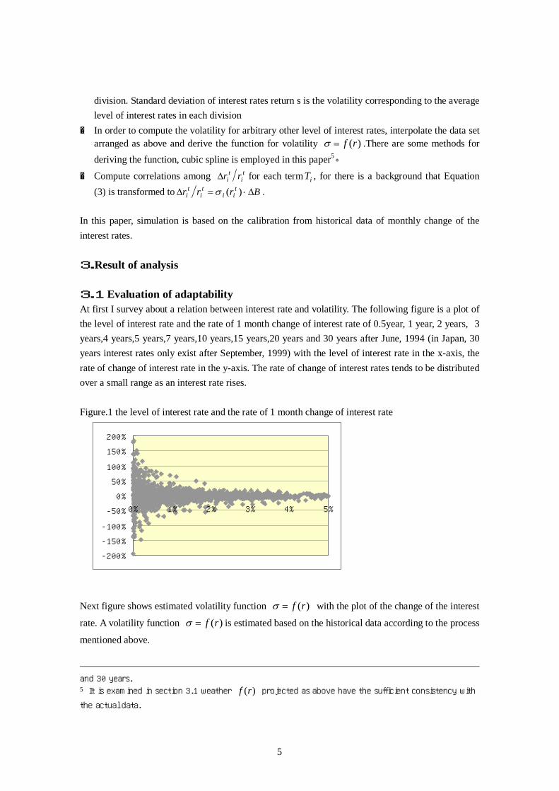
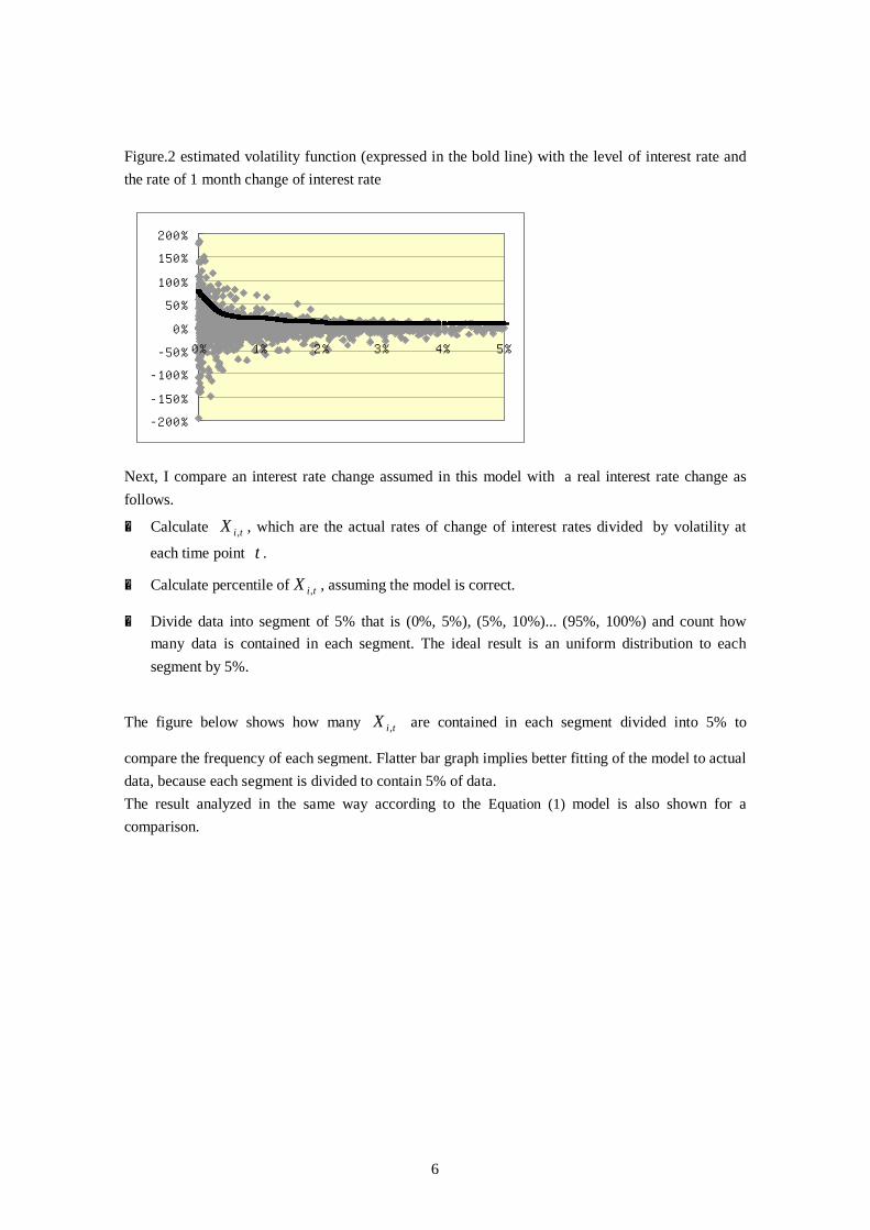
In this paper, simulation is based on the calibration from historical data of monthly change of the interest rates. ３．Result of analysis ３．１ Evaluation of adaptability At first I survey about a relation between interest rate and volatility. The following figure is a plot of the level of interest rate and the rate of 1 month change of interest rate of 0.5year, 1 year, 2 years, 3 years,4 years,5 years,7 years,10 years,15 years,20 years and 30 years after June, 1994 (in Japan, 30 years interest rates only exist after September, 1999) with the level of interest rate in the x-axis, the rate of change of interest rate in the y-axis. The rate of change of interest rates tends to be distributed over a small range as an interest rate rises. Figure.1 the level of interest rate and the rate of 1 month change of interest rate

Next figure shows estimated volatility function )(rf with the plot of the change of the interest

rate. A volatility function )(rf is estimated based on the historical data according to the process

mentioned above.

and 30 years. 5 It is examined in section 3.1 weather )(rf projected as above have the sufficient consistency with

the actual data.

-200%

-150%

-100%

-50%

0%

50%

100%

150%

200%

0% 1% 2% 3% 4% 5%

6

Figure.2 estimated volatility function (expressed in the bold line) with the level of interest rate and the rate of 1 month change of interest rate Next, I compare an interest rate change assumed in this model with a real interest rate change as follows.

① Calculate tiX , , which are the actual rates of change of interest rates divided by volatility at

each time point t .

② Calculate percentile of tiX , , assuming the model is correct.

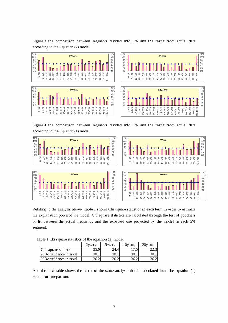
③ Divide data into segment of 5% that is (0%, 5%), (5%, 10%)... (95%, 100%) and count how many data is contained in each segment. The ideal result is an uniform distribution to each segment by 5%.

The figure below shows how many tiX , are contained in each segment divided into 5% to

compare the frequency of each segment. Flatter bar graph implies better fitting of the model to actual data, because each segment is divided to contain 5% of data. The result analyzed in the same way according to the Equation (1) model is also shown for a comparison.

-200%

-150%

-100%

-50%

0%

50%

100%

150%

200%

0% 1% 2% 3% 4% 5%

7

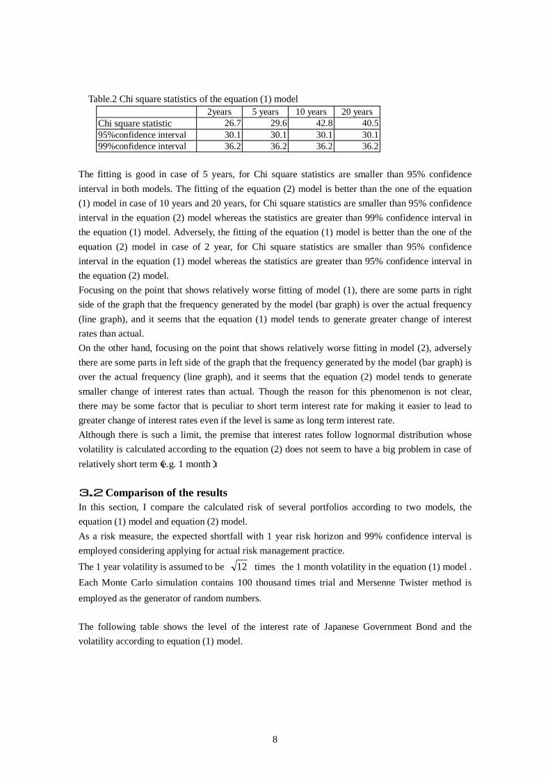
Figure.3 the comparison between segments divided into 5% and the result from actual data according to the Equation (2) model Figure.4 the comparison between segments divided into 5% and the result from actual data according to the Equation (1) model Relating to the analysis above, Table.1 shows Chi square statistics in each term in order to estimate the explanation powerof the model. Chi square statistics are calculated through the test of goodness of fit between the actual frequency and the expected one projected by the model in each 5% segment.

Table.1 Chi square statistics of the equation (2) model 2years 5years 10years 20years

Chi square statistic 35.9 24.4 17.5 22.3 95%confidence interval 30.1 30.1 30.1 30.1 99%confidence interval 36.2 36.2 36.2 36.2

And the next table shows the result of the same analysis that is calculated from the equation (1) model for comparison.

2Years

0%2%4%6%8%

10%12%

0-5%

5-1

0%

10-1

5%

15-2

0%

20-2

5%

25-3

0%

30-3

5%

35-4

0%

40-4

5%

45-5

0%

50-5

5%

55-6

0%

60-6

5%

65-7

0%

70-7

5%

75-8

0%

80-8

5%

85-9

0%

90-9

5%

95-

100%

0%2%4%6%8%10%12%

5Years

0%2%4%6%8%

10%12%

0-5%

5-1

0%

10-1

5%

15-2

0%

20-2

5%

25-3

0%

30-3

5%

35-4

0%

40-4

5%

45-5

0%

50-5

5%

55-6

0%

60-6

5%

65-7

0%

70-7

5%

75-8

0%

80-8

5%

85-9

0%

90-9

5%

95-

100%

0%2%4%6%8%10%12%

10Years

0%2%4%6%8%

10%12%

0-5

%

5-10

%

10-

15%

15-

20%

20-

25%

25-

30%

30-

35%

35-

40%

40-

45%

45-

50%

50-

55%

55-

60%

60-

65%

65-

70%

70-

75%

75-

80%

80-

85%

85-

90%

90-

95%

95-

100%

0%2%4%6%8%10%12%

20Years

0%2%4%6%8%

10%12%

0-5%

5-1

0%

10-1

5%

15-2

0%

20-2

5%

25-3

0%

30-3

5%

35-4

0%

40-4

5%

45-5

0%

50-5

5%

55-6

0%

60-6

5%

65-7

0%

70-7

5%

75-8

0%

80-8

5%

85-9

0%

90-9

5%

95-

100%

0%2%4%6%8%10%12%

5Years

0%2%4%6%8%

10%12%

0-5

%

5-10

%

10-

15%

15-

20%

20-

25%

25-

30%

30-

35%

35-

40%

40-

45%

45-

50%

50-

55%

55-

60%

60-

65%

65-

70%

70-

75%

75-

80%

80-

85%

85-

90%

90-

95%

95-1

00%

0%2%4%6%8%10%12%

2Years

0%2%4%6%8%

10%12%

0-5%

5-10

%

10-

15%

15-

20%

20-

25%

25-

30%

30-

35%

35-

40%

40-

45%

45-

50%

50-

55%

55-

60%

60-

65%

65-

70%

70-

75%

75-

80%

80-

85%

85-

90%

90-

95%

95-1

00%

0%2%4%6%8%10%12%

10Years

0%2%4%6%8%

10%12%

0-5

%

5-10

%

10-

15%

15-

20%

20-

25%

25-

30%

30-

35%

35-

40%

40-

45%

45-

50%

50-

55%

55-

60%

60-

65%

65-

70%

70-

75%

75-

80%

80-

85%

85-

90%

90-

95%

95-1

00%

0%2%4%6%8%10%12%

20Years

0%2%4%6%8%

10%12%

0-5%

5-1

0%

10-1

5%

15-2

0%

20-2

5%

25-3

0%

30-3

5%

35-4

0%

40-4

5%

45-5

0%

50-5

5%

55-6

0%

60-6

5%

65-7

0%

70-7

5%

75-8

0%

80-8

5%

85-9

0%

90-9

5%

95-

100%

0%2%4%6%8%10%12%

8

Table.2 Chi square statistics of the equation (1) model 2years 5 years 10 years 20 years

Chi square statistic 26.7 29.6 42.8 40.5 95%confidence interval 30.1 30.1 30.1 30.1 99%confidence interval 36.2 36.2 36.2 36.2

The fitting is good in case of 5 years, for Chi square statistics are smaller than 95% confidence interval in both models. The fitting of the equation (2) model is better than the one of the equation (1) model in case of 10 years and 20 years, for Chi square statistics are smaller than 95% confidence interval in the equation (2) model whereas the statistics are greater than 99% confidence interval in the equation (1) model. Adversely, the fitting of the equation (1) model is better than the one of the equation (2) model in case of 2 year, for Chi square statistics are smaller than 95% confidence interval in the equation (1) model whereas the statistics are greater than 95% confidence interval in the equation (2) model. Focusing on the point that shows relatively worse fitting of model (1), there are some parts in right side of the graph that the frequency generated by the model (bar graph) is over the actual frequency (line graph), and it seems that the equation (1) model tends to generate greater change of interest rates than actual. On the other hand, focusing on the point that shows relatively worse fitting in model (2), adversely there are some parts in left side of the graph that the frequency generated by the model (bar graph) is over the actual frequency (line graph), and it seems that the equation (2) model tends to generate smaller change of interest rates than actual. Though the reason for this phenomenon is not clear, there may be some factor that is peculiar to short term interest rate for making it easier to lead to greater change of interest rates even if the level is same as long term interest rate. Although there is such a limit, the premise that interest rates follow lognormal distribution whose volatility is calculated according to the equation (2) does not seem to have a big problem in case of relatively short term（e.g. 1 month）. ３．２ Comparison of the results In this section, I compare the calculated risk of several portfolios according to two models, the equation (1) model and equation (2) model. As a risk measure, the expected shortfall with 1 year risk horizon and 99% confidence interval is employed considering applying for actual risk management practice.

The 1 year volatility is assumed to be 12 times the 1 month volatility in the equation (1) model . Each Monte Carlo simulation contains 100 thousand times trial and Mersenne Twister method is employed as the generator of random numbers. The following table shows the level of the interest rate of Japanese Government Bond and the volatility according to equation (1) model.

9

Table.3

maturity yield volatility 99percrntile equation (1) model

upper lower 0.5y 0.37% 264.67% 439.15% 0.00% 1y 0.53% 206.26% 131.22% 0.00% 2y 0.83% 112.21% 16.66% 0.04% 3y 1.00% 88.46% 10.65% 0.09% 4y 1.21% 70.60% 8.00% 0.18% 5y 1.41% 65.46% 8.09% 0.25% 7y 1.72% 53.70% 7.22% 0.41% 10y 1.96% 34.59% 4.94% 0.78% 15y 2.24% 29.79% 4.96% 1.01% 20y 2.41% 26.43% 4.87% 1.19% 30y 2.70% 26.35% 5.45% 1.34%

As of 31 Jul 2006 Volatility is calculated as 12 times the standard deviation of monthly rate of change from September 1999 to July 2006. Upper and lower 99percentile values from lognormal distribution are estimated for 67.2exp or

67.2exp times the current interest rate respectively. In the table above, the column of upper 99percrntile indicates that the model tend to generate extremely large interest rates especially in short terms. Starting from the 0.5 year and 1 year, whose interest rates exceed 100%, 2 years and 3 years interest rates exceed 10%, and so on. I calculate the risk in real portfolio using both models next and compare the result. In this paper, the portfolio is assumed to be composed of discount bonds and discount liabilities that vary in maturity. And "short term" ," middle term" , "long term" and " ultra long term" mean 2 years, 5years, 10years and 30 years respectively. Case.1 calculation of risk of bonds portfolio Risks are calculated for the assets portfolio as follows. Each bond is assumed to be held in same volume in the mixed portfolio after the sample 1-4. 1-1 short term bonds portfolio 1-2 middle term bonds portfolio 1-3 long term bonds portfolio 1-4 ultra long term bonds portfolio 1-5 portfolio of short term bonds and middle term bonds 1-6 portfolio of short term bonds and long term bonds 1-7 portfolio of short term bonds and ultra long term bonds 1-8 portfolio of middle term bonds and long term bonds 1-9 portfolio of middle term bonds and ultra long term bonds

10

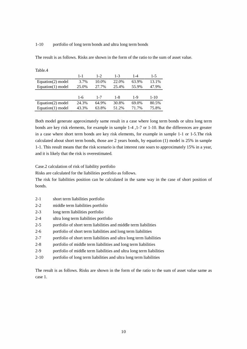
1-10 portfolio of long term bonds and ultra long term bonds The result is as follows. Risks are shown in the form of the ratio to the sum of asset value. Table.4 1-1 1-2 1-3 1-4 1-5 Equation(2) model 3.7% 10.0% 22.0% 63.9% 13.1% Equation(1) model 25.0% 27.7% 25.4% 55.9% 47.9% 1-6 1-7 1-8 1-9 1-10 Equation(2) model 24.3% 64.9% 30.8% 69.0% 80.5% Equation(1) model 43.3% 63.8% 51.2% 71.7% 75.8%

Both model generate approximately same result in a case where long term bonds or ultra long term bonds are key risk elements, for example in sample 1-4 ,1-7 or 1-10. But the differences are greater in a case where short term bonds are key risk elements, for example in sample 1-1 or 1-5.The risk calculated about short term bonds, those are 2 years bonds, by equation (1) model is 25% in sample 1-1. This result means that the risk scenario is that interest rate soars to approximately 15% in a year, and it is likely that the risk is overestimated. Case.2 calculation of risk of liability portfolio Risks are calculated for the liabilities portfolio as follows. The risk for liabilities position can be calculated in the same way in the case of short position of bonds. 2-1 short term liabilities portfolio 2-2 middle term liabilities portfolio 2-3 long term liabilities portfolio 2-4 ultra long term liabilities portfolio 2-5 portfolio of short term liabilities and middle term liabilities 2-6 portfolio of short term liabilities and long term liabilities 2-7 portfolio of short term liabilities and ultra long term liabilities 2-8 portfolio of middle term liabilities and long term liabilities 2-9 portfolio of middle term liabilities and ultra long term liabilities 2-10 portfolio of long term liabilities and ultra long term liabilities The result is as follows. Risks are shown in the form of the ratio to the sum of asset value same as case 1.

11

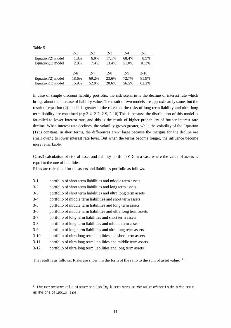
Table.5 2-1 2-2 2-3 2-4 2-5 Equation(2) model 1.8% 6.9% 17.1% 68.4% 8.5% Equation(1) model 2.8% 7.4% 13.4% 51.0% 10.2% 2-6 2-7 2-8 2-9 2-10 Equation(2) model 18.6% 69.2% 23.6% 72.7% 81.9% Equation(1) model 15.9% 52.9% 20.6% 56.5% 62.2%

In case of simple discount liability portfolio, the risk scenario is the decline of interest rate which brings about the increase of liability value. The result of two models are approximately same, but the result of equation (2) model is greater in the case that the risks of long term liability and ultra long term liability are contained (e.g.2-4, 2-7, 2-9, 2-10).This is because the distribution of this model is fat-tailed to lower interest rate, and this is the result of higher probability of further interest rate decline. When interest rate declines, the volatility grows greater, while the volatility of the Equation (1) is constant. In short terms, the differences aren't large because the margins for the decline are small owing to lower interest rate level. But when the terms become longer, the influence become more remarkable. Case.3 calculation of risk of asset and liability portfolio（1）- in a case where the value of assets is equal to the one of liabilities. Risks are calculated for the assets and liabilities portfolio as follows. 3-1 portfolio of short term liabilities and middle term assets 3-2 portfolio of short term liabilities and long term assets 3-3 portfolio of short term liabilities and ultra long term assets 3-4 portfolio of middle term liabilities and short term assets 3-5 portfolio of middle term liabilities and long term assets 3-6 portfolio of middle term liabilities and ultra long term assets 3-7 portfolio of long term liabilities and short term assets 3-8 portfolio of long term liabilities and middle term assets 3-9 portfolio of long term liabilities and ultra long term assets 3-10 portfolio of ultra long term liabilities and short term assets 3-11 portfolio of ultra long term liabilities and middle term assets 3-12 portfolio of ultra long term liabilities and long term assets The result is as follows. Risks are shown in the form of the ratio to the sum of asset value. 6。

6 The net present value of asset and liability is zero because the value of asset side is the same

as the one of liability side.

12

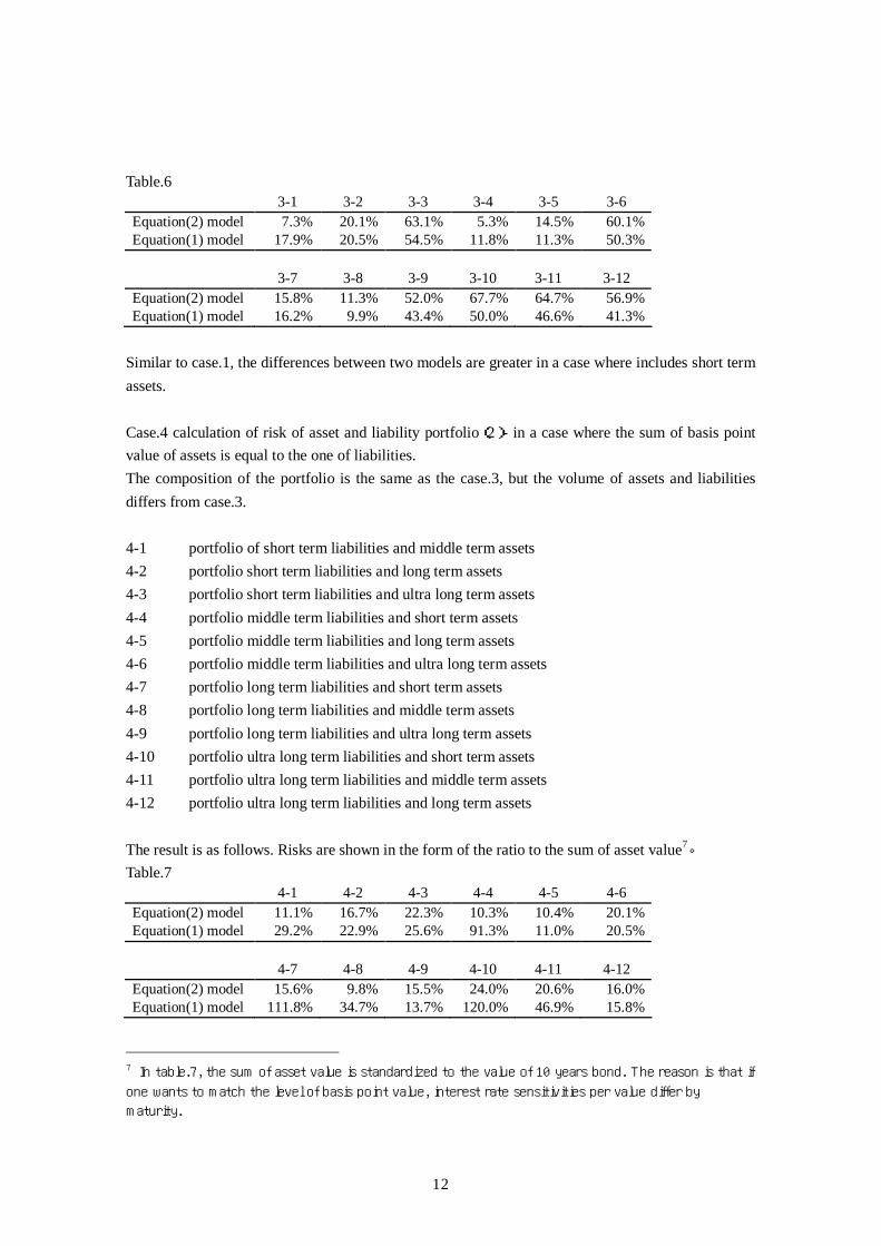
Table.6 3-1 3-2 3-3 3-4 3-5 3-6 Equation(2) model 7.3% 20.1% 63.1% 5.3% 14.5% 60.1% Equation(1) model 17.9% 20.5% 54.5% 11.8% 11.3% 50.3% 3-7 3-8 3-9 3-10 3-11 3-12 Equation(2) model 15.8% 11.3% 52.0% 67.7% 64.7% 56.9% Equation(1) model 16.2% 9.9% 43.4% 50.0% 46.6% 41.3%

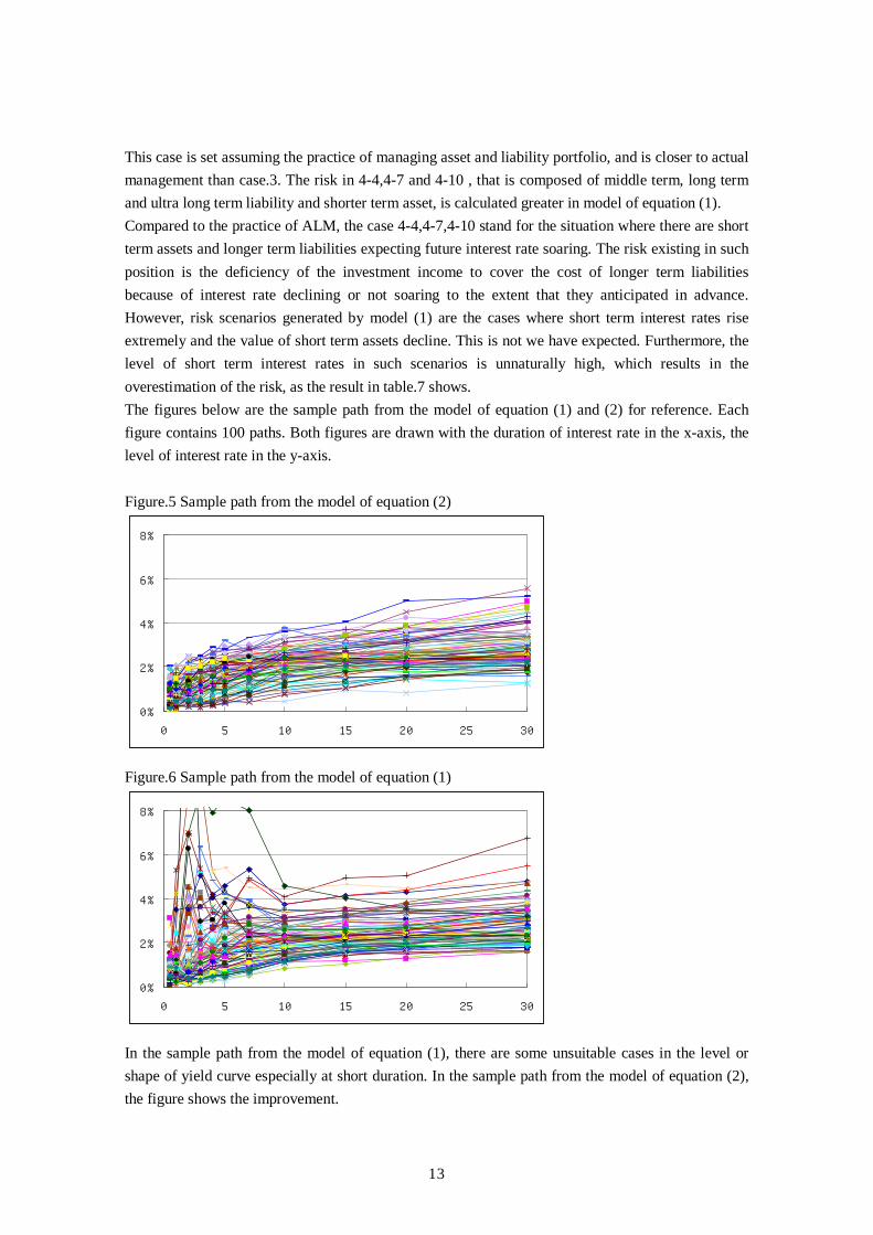
Similar to case.1, the differences between two models are greater in a case where includes short term assets. Case.4 calculation of risk of asset and liability portfolio（2）- in a case where the sum of basis point value of assets is equal to the one of liabilities. The composition of the portfolio is the same as the case.3, but the volume of assets and liabilities differs from case.3. 4-1 portfolio of short term liabilities and middle term assets 4-2 portfolio short term liabilities and long term assets 4-3 portfolio short term liabilities and ultra long term assets 4-4 portfolio middle term liabilities and short term assets 4-5 portfolio middle term liabilities and long term assets 4-6 portfolio middle term liabilities and ultra long term assets 4-7 portfolio long term liabilities and short term assets 4-8 portfolio long term liabilities and middle term assets 4-9 portfolio long term liabilities and ultra long term assets 4-10 portfolio ultra long term liabilities and short term assets 4-11 portfolio ultra long term liabilities and middle term assets 4-12 portfolio ultra long term liabilities and long term assets The result is as follows. Risks are shown in the form of the ratio to the sum of asset value7。 Table.7 4-1 4-2 4-3 4-4 4-5 4-6 Equation(2) model 11.1% 16.7% 22.3% 10.3% 10.4% 20.1% Equation(1) model 29.2% 22.9% 25.6% 91.3% 11.0% 20.5% 4-7 4-8 4-9 4-10 4-11 4-12 Equation(2) model 15.6% 9.8% 15.5% 24.0% 20.6% 16.0% Equation(1) model 111.8% 34.7% 13.7% 120.0% 46.9% 15.8%

7 In table.7, the sum of asset value is standardized to the value of 10 years bond. The reason is that if

one wants to match the level of basis point value, interest rate sensitivities per value differ by

maturity.

13

This case is set assuming the practice of managing asset and liability portfolio, and is closer to actual management than case.3. The risk in 4-4,4-7 and 4-10 , that is composed of middle term, long term and ultra long term liability and shorter term asset, is calculated greater in model of equation (1). Compared to the practice of ALM, the case 4-4,4-7,4-10 stand for the situation where there are short term assets and longer term liabilities expecting future interest rate soaring. The risk existing in such position is the deficiency of the investment income to cover the cost of longer term liabilities because of interest rate declining or not soaring to the extent that they anticipated in advance. However, risk scenarios generated by model (1) are the cases where short term interest rates rise extremely and the value of short term assets decline. This is not we have expected. Furthermore, the level of short term interest rates in such scenarios is unnaturally high, which results in the overestimation of the risk, as the result in table.7 shows. The figures below are the sample path from the model of equation (1) and (2) for reference. Each figure contains 100 paths. Both figures are drawn with the duration of interest rate in the x-axis, the level of interest rate in the y-axis. Figure.5 Sample path from the model of equation (2) Figure.6 Sample path from the model of equation (1) In the sample path from the model of equation (1), there are some unsuitable cases in the level or shape of yield curve especially at short duration. In the sample path from the model of equation (2), the figure shows the improvement.

0%

2%

4%

6%

8%

0 5 10 15 20 25 30

0%

2%

4%

6%

8%

0 5 10 15 20 25 30

14

４．Conclusion Under the extremely low interest rate environment in Japan, the difficulty in applying an existing model especially for risk management has been pointed out. In this paper, the structure in which volatility varies according to the current interest rate is incorporated into traditional model with lognormal distribution. The model overcomes drawbacks that the risk of interest rate soaring is overestimated especially in short durations and MAKES it possible to calculate interest rate risk more accurately and closely to actual market behavior. The result of this model may also be used in the countries except Japan in case ultra low interest rate market environment will occur. In addition, the model may be used not only in modeling of interest rate but also of the phenomenon whose possibility is almost zero but not negative (for example, the mortality in younger ages). Outstanding issues and future steps are as follows. The behavior of short term interest rates should be scrutinized when they become the same level as current long term interest rates. In case there are remarkable differences between those rates in their behavior even if they are almost same interest rate level, it needs further analysis to incorporate the other elements into risk model. When interest rate market environment will back to the ordinary situation in Japan, the utilization of historical data under extremely low interest rate environment would be a challenging problem, too. References [1] Greg M. Gupton, Christopher C.Finger and Mickey Bhatia[1997] CreditMetricsTM Technical

Document, J.P.Morgan [2] Masaaki Kijima[1998] Quantifying financial risk(Value at Risk) , Kinzai [3] M. Matsumoto and T. Nishimura [1998] Mersenne Twister, ACM Transcript on Modeling and

Computer Simulation, Vol.8 No.2 [4] Artzner, P., F. Delbaen, J. M. Eber, and D. Heath [1999] Coherent Measures of Risk,

Mathematical Finance, Vol. 9, No. 3, pp.203-228. [5] Jorge Mina and Jerry Yi Xiao[2001] Return to RiskMetrics: The Evolution of a

Standard ,RiskMetrics Group [6] Yasuhiro Yamai and Toshinao Yoshiba [2002] On the Validity of Value-at-Risk: Comparative

Analyses with Expected Shortfall , Monetary and Economic Studies Vol.20, No.1 , Institute for monetary and economic studies, Bank of Japan

[7] Masaaki Hamano, Yuji Morimoto and Shigeru Taguchi[2003] International accounting standards of insurance and market value evaluation of insurance liabilities , Actuary Journal Vol.48 The Institute of Actuaries of Japan

[8] IAA Insurer Solvency Assessment Working Party [2004] “A Global Framework for Insurer Solvency Assessment”

[9] Hideyuki Torii[2004] Now and the future of the system for VaR and EaR（the first part）, Numerical Technologies

[10] Hideyuki Torii [2005] Now and the future of the system for VaR and EaR（the latter part）, Numerical Technologies