IEEE TRANSACTIONS ON AUTOMATIC CONTROL, VOL. …robotics.eecs.berkeley.edu/~sastry/pubs/OldSastryALL/Sinopoli... · SINOPOLI et al.: KALMAN FILTERING WITH INTERMITTENT OBSERVATIONS

IEEE TRANSACTIONS ON AUTOMATIC CONTROL, VOL. 49, NO. 9, SEPTEMBER 2004 1453

Kalman Filtering With Intermittent ObservationsBruno Sinopoli, Student Member, IEEE, Luca Schenato, Member, IEEE, Massimo Franceschetti, Member, IEEE,

Kameshwar Poolla, Member, IEEE, Michael I. Jordan, Senior Member, IEEE, and Shankar S. Sastry, Fellow, IEEE

Abstract—Motivated by navigation and tracking applicationswithin sensor networks, we consider the problem of performingKalman filtering with intermittent observations. When data travelalong unreliable communication channels in a large, wireless,multihop sensor network, the effect of communication delays andloss of information in the control loop cannot be neglected. Weaddress this problem starting from the discrete Kalman filteringformulation, and modeling the arrival of the observation as arandom process. We study the statistical convergence propertiesof the estimation error covariance, showing the existence of acritical value for the arrival rate of the observations, beyondwhich a transition to an unbounded state error covariance occurs.We also give upper and lower bounds on this expected state errorcovariance.

Index Terms—Kalman estimation, missing observation, onlineadaptive filtering, sensor networks, stability.

I. INTRODUCTION

ADVANCES in very large-scale integration and micro-electromechanical system technology have boosted the

development of micro sensor integrated systems. Such sys-tems combine computing, storage, radio technology, and energysource on a single chip [1], [2]. When distributed over a widearea, networks of sensors can perform a variety of tasks thatrange from environmental monitoring and military surveil-lance, to navigation and control of a moving vehicle [3]–[5].A common feature of these systems is the presence of signif-icant communication delays and data loss across the network.From the point of view of control theory, significant delay isequivalent to loss, as data needs to arrive to its destinationin time to be used for control. In short, communication andcontrol become tightly coupled such that the two issues cannotbe addressed independently.

Consider, for example, the problem of navigating a vehiclebased on the estimate from a sensor web of its current positionand velocity. The measurements underlying this estimate canbe lost or delayed due to the unreliability of the wireless links.What is the amount of data loss that the control loop can tolerateto reliably perform the navigation task? Can communicationprotocols be designed to satisfy this constraint? At Berkeley, wehave faced these kind of questions in building sensor networksfor pursuit evasion games as part of the network of embeddedsystems technology (NEST) project [2]. Practical advances in

Manuscript received May 21, 2003; revised December 5, 2003 and March 8,2003. Recommended by Guest Editors P. Antsaklis and J. Baillieul. This workwas supported by the Defense Advanced Research Projects Agency under GrantF33615-01-C-1895.

The authors are with the Department of Electrical Engineering and ComputerSciences, the University of California, Berkeley, CA 94720 USA (e-mail: [email protected]).

Digital Object Identifier 10.1109/TAC.2004.834121

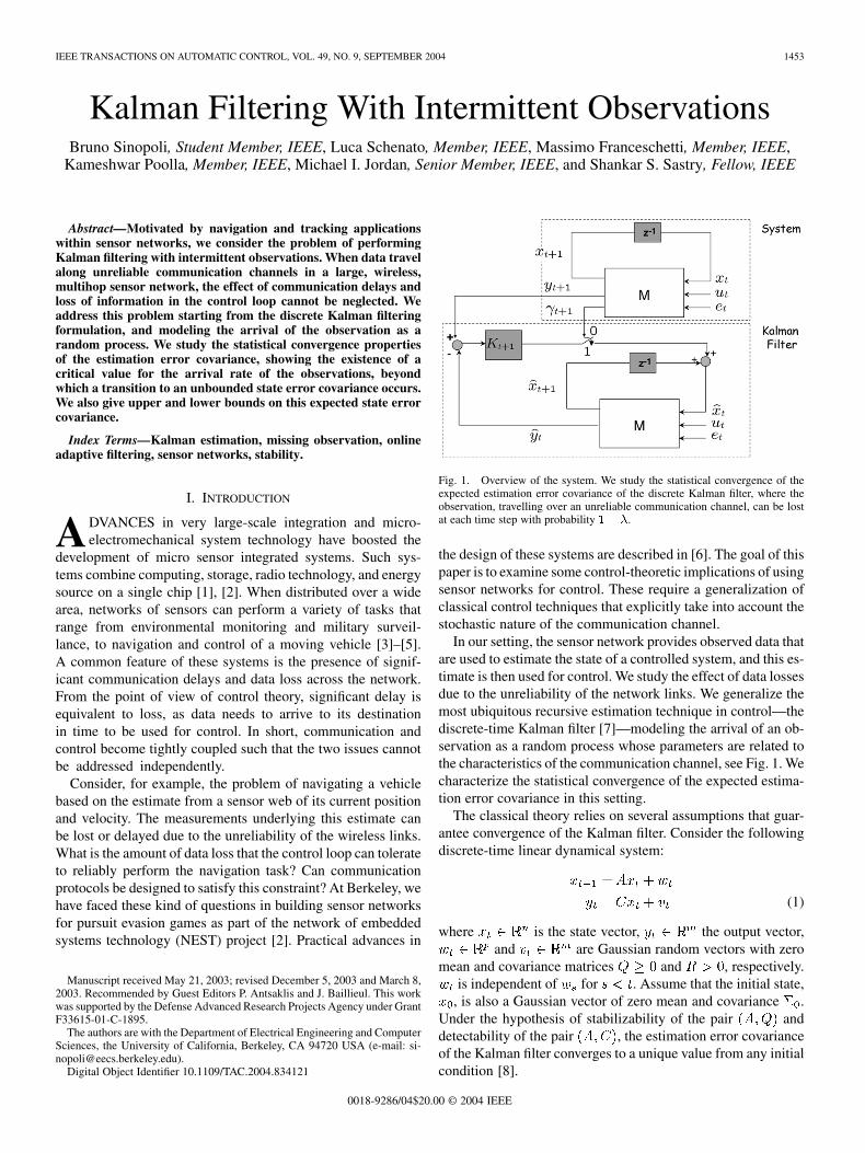
Fig. 1. Overview of the system. We study the statistical convergence of theexpected estimation error covariance of the discrete Kalman filter, where theobservation, travelling over an unreliable communication channel, can be lostat each time step with probability 1 � �.

the design of these systems are described in [6]. The goal of thispaper is to examine some control-theoretic implications of usingsensor networks for control. These require a generalization ofclassical control techniques that explicitly take into account thestochastic nature of the communication channel.

In our setting, the sensor network provides observed data thatare used to estimate the state of a controlled system, and this es-timate is then used for control. We study the effect of data lossesdue to the unreliability of the network links. We generalize themost ubiquitous recursive estimation technique in control—thediscrete-time Kalman filter [7]—modeling the arrival of an ob-servation as a random process whose parameters are related tothe characteristics of the communication channel, see Fig. 1. Wecharacterize the statistical convergence of the expected estima-tion error covariance in this setting.

The classical theory relies on several assumptions that guar-antee convergence of the Kalman filter. Consider the followingdiscrete-time linear dynamical system:

(1)

where is the state vector, the output vector,and are Gaussian random vectors with zero

mean and covariance matrices and , respectively.is independent of for . Assume that the initial state,

, is also a Gaussian vector of zero mean and covariance .Under the hypothesis of stabilizability of the pair anddetectability of the pair , the estimation error covarianceof the Kalman filter converges to a unique value from any initialcondition [8].

0018-9286/04$20.00 © 2004 IEEE

1454 IEEE TRANSACTIONS ON AUTOMATIC CONTROL, VOL. 49, NO. 9, SEPTEMBER 2004

These assumptions have been relaxed in various ways. Ex-tended Kalman filtering [8] attempts to cope with nonlinearitiesin the model; particle filtering [9] is also appropriate for non-linear models and additionally does not require the noise modelto be Gaussian. Recently, more general observation processeshave been studied. In particular, in [10] and [11], the case inwhich observations are randomly spaced in time according toa Poisson process has been studied, where the underlying dy-namics evolve in continuous time. These authors showed theexistence of a lower bound on the arrival rate of the observa-tions below which it is possible to maintain the estimation errorcovariance below a fixed value, with high probability. However,the results were restricted to scalar single-input–single-outputsystems.

We approach a similar problem within the framework of dis-crete time, and provide results for general -dimensional mul-tiple-input–multiple-output (MIMO) systems. In particular, weconsider a discrete-time system in which the arrival of an ob-servation is a Bernoulli process with parameter ,and, rather than asking for the estimation error covariance tobe bounded with high probability, we study the asymptotic be-havior (in time) of its average. Our main contribution is to showthat, depending on the eigenvalues of the matrix , and on thestructure of the matrix , there exists a critical value , suchthat if the probability of arrival of an observation at time is

, then the expectation of the estimation error covarianceis always finite (provided that the usual stabilizability and de-tectability hypotheses are satisfied). If , then the expec-tation of the estimation error covariance is unbounded. We giveexplicit upper and lower bounds on , and show that they aretight in some special cases.

Philosophically, this result can be seen as another manifes-tation of the well known uncertainty threshold principle [12],[13]. This principle states that optimum long-range control of adynamical system with uncertainty parameters is possible if andonly if the uncertainty does not exceed a given threshold. Theuncertainty is modeled as white noise scalar sequences actingon the system and control matrices. In our case, the result is foroptimal estimation, rather than optimal control, and the uncer-tainty is due to the random arrival of the observation, with therandomness arising from losses in the network.

Studies on filtering with intermittent observations can betracked back to Nahi [14] and Hadidi [15]. More recently, thisproblem has been studied using jump linear systems (JLSs)[16]. JLSs are stochastic hybrid systems characterized by lineardynamics and discrete regime transitions modeled as Markovchains. In [17], [18], and [19], the Kalman filter with missingobservations is modeled as a JLS switching between two dis-crete regimes: an open-loop configuration and a closed-loopone. Following this approach, these authors obtain convergencecriteria for the expected estimation error covariance. How-ever, they restrict their formulation to the steady-state case,where the Kalman gain is constant, and they do not assume toknow the switching sequence. The resulting process is widesense stationary [20], and this makes the exact computation ofthe transition probability and state error covariance possible.Other work on optimal, constant gain filtering can be foundin the work of Wang et al. [21], who included the presence of

system parameters uncertainty besides missing observations,and Smith et al. [22], who considered multiple filters fusion.Instead, we consider the general case of time varying Kalmangain. In presence of missing observations, this filter has asmaller linear minimum mean square error (LMMSE) than itsstatic counterpart, as it is detailed in Section II.

The general case of time-varying Kalman filter with intermit-tent observations was also studied by Fortmann et al. [23], whoderived stochastic equations for the state covariance error. How-ever, they do not statistically characterize its convergence andprovide only numerical evidence of the transition to instability,leaving a formal characterization of this as an open problem,which is addressed in this paper. A somewhat different formula-tion was considered in [24], where the observations arrival havea bounded delay.

Finally, we point out that our analysis can also be viewed asan instance of expectation–maximization (EM) theory. EM isa general framework for doing maximum likelihood estimationin missing-data models [25]. Lauritzen [26] shows how EM canbe used for general graphical models. In our case, however, thegraph structure is a function of the missing data, as there is onegraph for each pattern of missing data.

The paper is organized as follows. In Section II, we formalizethe problem of Kalman filtering with intermittent observations.In Section III, we provide upper and lower bounds on the ex-pected estimation error covariance of the Kalman filter, and findthe conditions on the observation arrival probability for whichthe upper bound converges to a fixed point, and for which thelower bound diverges. Section IV describes some special casesand gives an intuitive understanding of the results. In Section V,we compare our approach to previous ones [18] based on jumplinear systems. Finally, in Section VI, we state our conclusionsand give directions for future work.

II. PROBLEM FORMULATION

Consider the canonical state estimation problem. We definethe arrival of the observation at time as a binary random vari-able , with probability distribution , and withindependent of if . The output noise is defined in thefollowing way:

for some . Therefore, the variance of the observation at timeis if is 1, and otherwise. In reality the absence of obser-vation corresponds to the limiting case of . Our approachis to rederive the Kalman filter equations using a “dummy” ob-servation with a given variance when the real observation doesnot arrive, and then take the limit as .

First, let us define

(2)

(3)

(4)

(5)

(6)

SINOPOLI et al.: KALMAN FILTERING WITH INTERMITTENT OBSERVATIONS 1455

where we have defined the vectors and. It is easy to see that

(7)

(8)

and it follows that the random variables and , con-ditioned on the output and on the arrivals , are jointlyGaussian with mean

and covariance

Hence, the Kalman filter equations are modified as follows:

(9)

(10)

(11)

(12)

Taking the limit as , the update (11) and (12) can berewritten as follows:

(13)

(14)

where is the Kalmangain matrix for the standard ARE. Note that performing thislimit corresponds exactly to propagating the previous state whenthere is no observation update available at time . We also pointout the main difference from the standard Kalman filter formu-lation: Both and are now random variables,being a function of , which is itself random.

It is important to stress that (13) and (14) give the minimumstate-error variance filter given the observations and theirarrival sequence , i.e. .As a consequence, the filter proposed in this paper is neces-sarily time-varying and stochastic since it depends on the arrivalsequence. The filters that have been proposed so far using JLStheory [17], [19] give the minimum state error variance filtersassuming that only the observations and the knowledge onthe last arrival are available, i.e. .Therefore, the filter given by (13) and (14) gives a better per-formance than its JLS counterparts, since it exploits additionalinformation regarding the arrival sequence.

Given the new formulation, we now study the Riccati equa-tion of the state error covariance matrix in the specific case when

the arrival process of the observation is time-independent, i.e.,for all time. This will allow us to provide deterministic

upper and lower bounds on its expectation. We then characterizethe convergence of these upper and lower bounds, as a functionof the arrival probability of the observation.

III. CONVERGENCE CONDITIONS AND TRANSITION

TO INSTABILITY

It is easy to verify that the modified Kalman filter formulationin (10) and (14) can be rewritten as follows:

(15)

where we use the simplified notation . Since thesequence is random, the modified Kalman filter iterationis stochastic and cannot be determined offline. Therefore, onlystatistical properties can be deduced.

In this section, we show the existence of a critical valuefor the arrival probability of the observation update, such that for

the mean state covariance is bounded for all initialconditions, and for the mean state covariance divergesfor some initial condition. We also find a lower bound , andupper bound , for the critical probability , i.e., .The lower bound is expressed in closed form; the upper bound isthe solution of a linear matrix inequality (LMI). In some specialcases the two bounds coincide, giving a tight estimate. Finally,we present numerical algorithms to compute a lower bound ,and upper bound , for , when it is bounded.

First, we define the modified algebraic Riccati equation(MARE) for the Kalman filter with intermittent observations asfollows:

(16)

Our results derive from two principal facts: The first is that con-cavity of the modified algebraic Riccati equation for our filterwith intermittent observations allows use of Jensen’s inequalityto find an upper bound on the mean state covariance; the secondis that all the operators we use to estimate upper and lowerbounds are monotonically increasing, therefore, if a fixed pointexists, it is also stable.

We formally state all main results in form of theorems.Omitted proofs appear in the Appendix. The first theoremexpresses convergence properties of the MARE.

Theorem 1: Consider the operator, where ,

. Suppose there exists a matrix and apositive–definite matrix such that

and

Then

a) for any initial condition , the MARE converges,and the limit is independent of the initial condition

b) is the unique positive–semidefinite fixed point of theMARE.

The next theorem states the existence of a sharp transition.


Theorem 2: If is controllable, is de-tectable, and is unstable, then there exists a suchthat

for and (17)

for and (18)

where depends on the initial condition .1

The next theorem gives upper and lower bounds for the crit-ical probability .

Theorem 3: Let

(19)

(20)

where and are the eigenvalues of . Then

(21)

Finally, the following theorem gives an estimate of the limitof the mean covariance matrix , when this is bounded.

Theorem 4: Assume that is controllable, isdetectable and , where is defined in Theorem 4. Then

(22)

where and , where andare solution of the respective algebraic equations

and .The previous theorems give lower and upper bounds for both

the critical probability and for the mean error covariance. The lower bound is expressed in closed form. We now

resort to numerical algorithms for the computation of the re-maining bounds , and .

The computation of the upper bound can be reformulatedas the iteration of an LMI feasibility problem. To establish this,we need the following theorem.

Theorem 5: If is controllable and is de-tectable, then the following statements are equivalent.

a) such thatb) , such thatc) and such that

Proof: a) b) If exists, then byLemma 1(g). Let . Thenwhich proves the statement.

b) a) Clearly which proves thestatement.

b) c) Let , then

1We use the notation lim A = +1 when the sequence A � 0 is notbounded, i.e., there is no matrix M � 0 such that A � M , 8t.

is equivalent to

where we used the Schur complement decomposition and thefact that .Using one more time the Schur complement decomposition onthe first element of the matrix we obtain

This is equivalent to

Let us consider the change of variable and, in which case the previous LMI is equivalent to

Since , then can be restricted to, which completes the theorem.

Combining Theorems 3 and 5, we immediately have the fol-lowing corollary.

Corollary 1: The upper bound is given by the solution ofthe following optimization problem:

This is a quasi-convex optimization problem in the variablesand the solution can be obtained by iterating LMI

feasibility problems and using bisection for the variable , asshown in [27].

The lower bound for the mean covariance matrix can beeasily obtained via standard Lyapunov Equation solvers. Theupper bound can be found by iterating the MARE or bysolving a semidefinite programming (SDP) problem as shownin the following.

Theorem 6: If , then the matrix is givenby

a) ; whereb)

subject to

Proof:

a) It follows directly from Theorem 1.


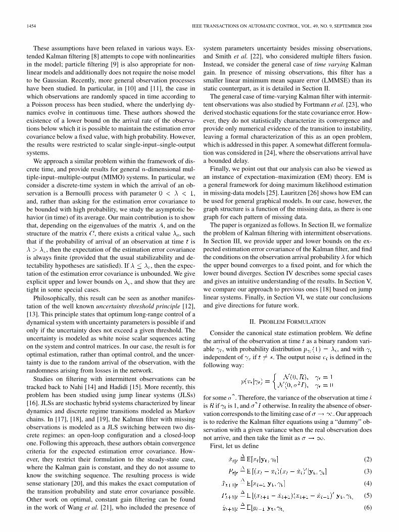
Fig. 2. Example of transition to instability in the scalar case. The dashed lineshows the asymptotic value of the lower bound ( �S), the solid line the asymptoticvalue of the upper bound ( �V ), and the dashed–dotted line shows the asymptote(� ).

b) It can be obtained by using the Schur complement de-composition on the equation . Clearly, thesolution belongs to the feasible set of theoptimization problem. We now show that the solution ofthe optimization problem is the fixed point of the MARE.Suppose it is not, i.e., solves the optimization problembut . Since is a feasible point of the op-

timization problem, then . However,

this implies that , which contra-dicts the hypothesis of optimality of matrix . Therefore,

and this concludes the theorem.

IV. SPECIAL CASES AND EXAMPLES

In this section, we present some special cases in which upperand lower bounds on the critical value coincide and give someexamples. From Theorem 1, it follows that if there exists asuch that is the zero matrix, then the convergence conditionof the MARE is for , where ,and are the eigenvalues of .

• C is invertible: In this case, a choice ofmakes . Note that the scalar case also falls under thiscategory. Fig. 2 shows a plot of the steady state of the upperand lower bounds versus in the scalar case. The discretetime LTI system used in this simulation has ,

, with and having zero mean and varianceand , respectively. For this system, we have

. The transition clearly appears in the figure,where we see that the steady-state value of both upperand lower bound tends to infinity as approaches . Thedashed line shows the lower bound, the solid line the upperbound, and the dashed–dotted line shows the asymptote.

• A has a single unstable eigenvalue: In this case, regard-less of the dimension of (and as long as the pairis detectable), we can use Kalman decomposition to bring

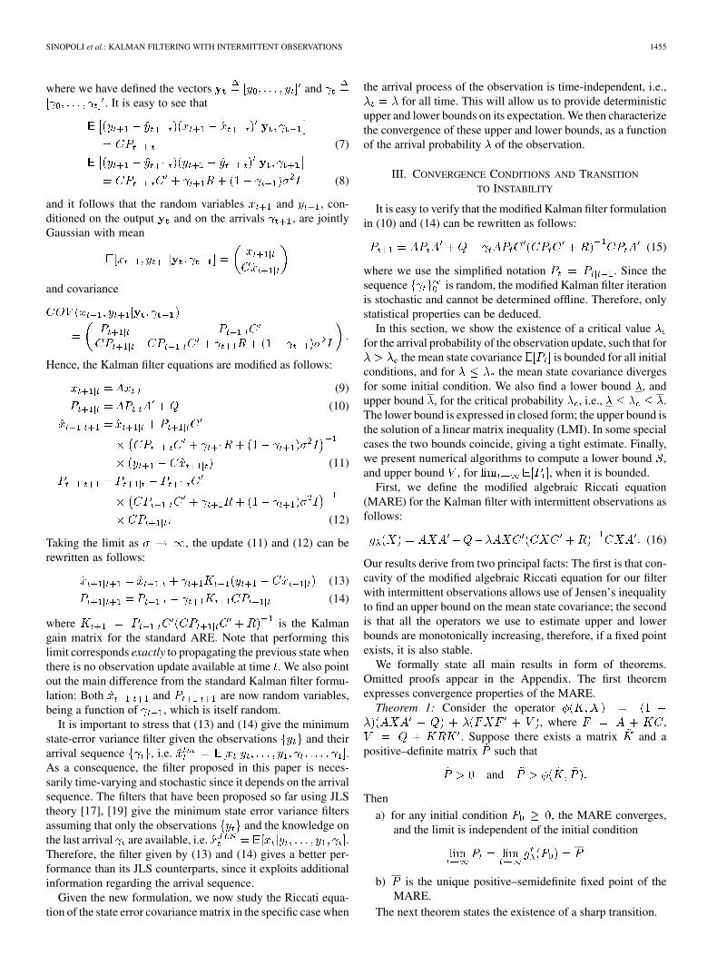
Fig. 3. Example of transition to instability with a single unstable eigenvaluein the MIMO case. The dashed line shows the asymptotic value of the trace oflower bound ( �S), the solid line the asymptotic value of trace of the upper bound( �V ), and the dashed–dotted line shows the asymptote (� ).

to zero the unstable part of and thereby obtain tightbounds. Fig. 3 shows a plot for the system

with and having zero mean and varianceand , respectively. This time, the asymptoticvalue for trace of upper and lower bound is plotted versus

. Once again .In general, cannot always be made zero and we have shown

that while a lower bound on can be written in closed form,an upper bound on is the result of a LMI. Fig. 4 shows anexample where upper and lower bounds have different conver-gence conditions. The system used for this simulation is

with and having zero mean and variance and, respectively.

Finally, in Fig. 5 we report results of another experiment,plotting the state estimation error for the scalar system usedabove at two similar values of , one being below and oneabove the critical value. We note a dramatic change in the errorat . The figure on the left shows the estimation errorwith . The figure on the right shows the estimation errorfor the same system evolution with . In the first case,the estimation error grows dramatically, making it practicallyuseless for control purposes. In the second case, a small increasein reduces the estimation error by approximately three ordersof magnitude.

V. STATIC VERSUS DYNAMIC KALMAN GAIN

In this section, we compare the performance of filtering withstatic and dynamic gain for a scalar discrete system. For thestatic estimator, we follow the jump linear system approach of


Fig. 5. Estimation error for � (left) below and (right) above the critical value.

Fig. 4. Transition to instability in the general case, with arbitrary A and C. Inthis case, lower and upper bounds do not have the same asymptote.

[18]. The scalar static estimator case has been also worked outin [28].

Consider the dynamic state estimator

(23)

where the Kalman gain is time-varying. Also consider thestatic state estimator

(24)

where the estimator gain is constant. If no data arrives, i.e.,, both estimators simply propagate the state estimate of

the previous time-step.The performance of the dynamic state estimator (23) has been

analyzed in the previous sections. The performance of staticstate estimator (24), instead, can be readily obtained using jumplinear system theory [16], [18]. To do so, let us consider the es-timator error . Substituting (1) for and(24) for , we obtain the dynamics of the estimation error

(25)

Using the same notation of [18, Ch. 6], where the author con-siders the general system

system (25) can be seen as jump linear system switching be-tween two states given by

where the noise covariance , the transition prob-ability matrix and the steady-state probability distribution

are given by


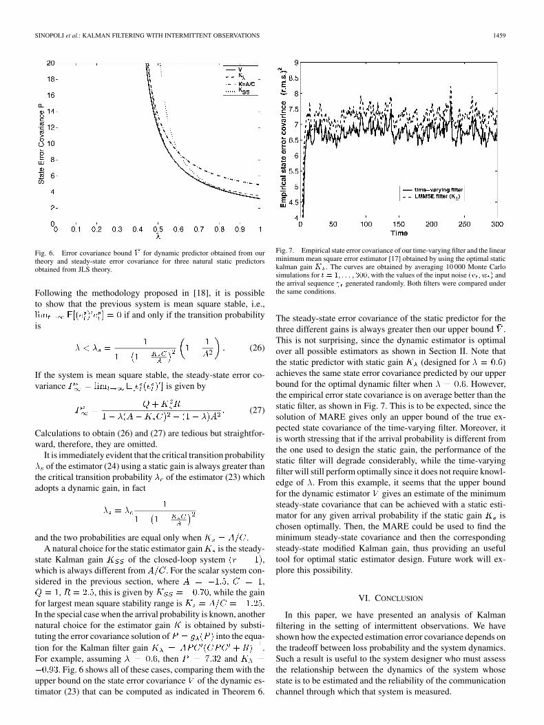
Fig. 6. Error covariance bound �V for dynamic predictor obtained from ourtheory and steady-state error covariance for three natural static predictorsobtained from JLS theory.

Following the methodology proposed in [18], it is possibleto show that the previous system is mean square stable, i.e.,

if and only if the transition probabilityis

(26)

If the system is mean square stable, the steady-state error co-variance is given by

(27)

Calculations to obtain (26) and (27) are tedious but straightfor-ward, therefore, they are omitted.

It is immediately evident that the critical transition probabilityof the estimator (24) using a static gain is always greater than

the critical transition probability of the estimator (23) whichadopts a dynamic gain, in fact

and the two probabilities are equal only when .A natural choice for the static estimator gain is the steady-

state Kalman gain of the closed-loop system ,which is always different from . For the scalar system con-sidered in the previous section, where , ,

, , this is given by , while the gainfor largest mean square stability range is .In the special case when the arrival probability is known, anothernatural choice for the estimator gain is obtained by substi-tuting the error covariance solution of into the equa-tion for the Kalman filter gain .For example, assuming , then and

. Fig. 6 shows all of these cases, comparing them with theupper bound on the state error covariance of the dynamic es-timator (23) that can be computed as indicated in Theorem 6.

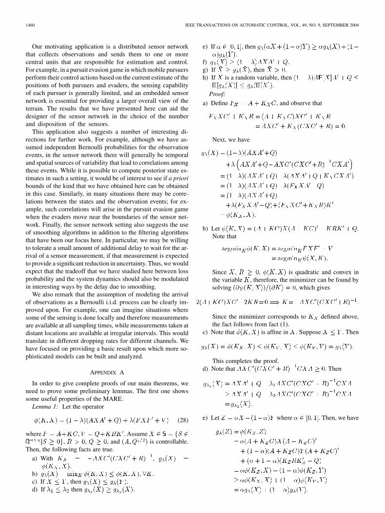
Fig. 7. Empirical state error covariance of our time-varying filter and the linearminimum mean square error estimator [17] obtained by using the optimal statickalman gain K . The curves are obtained by averaging 10 000 Monte Carlosimulations for t = 1; . . . ; 300, with the values of the input noise (v ; w ) andthe arrival sequence generated randomly. Both filters were compared underthe same conditions.

The steady-state error covariance of the static predictor for thethree different gains is always greater then our upper bound .This is not surprising, since the dynamic estimator is optimalover all possible estimators as shown in Section II. Note thatthe static predictor with static gain (designed for )achieves the same state error covariance predicted by our upperbound for the optimal dynamic filter when . However,the empirical error state covariance is on average better than thestatic filter, as shown in Fig. 7. This is to be expected, since thesolution of MARE gives only an upper bound of the true ex-pected state covariance of the time-varying filter. Moreover, itis worth stressing that if the arrival probability is different fromthe one used to design the static gain, the performance of thestatic filter will degrade considerably, while the time-varyingfilter will still perform optimally since it does not require knowl-edge of . From this example, it seems that the upper boundfor the dynamic estimator gives an estimate of the minimumsteady-state covariance that can be achieved with a static esti-mator for any given arrival probability if the static gain ischosen optimally. Then, the MARE could be used to find theminimum steady-state covariance and then the correspondingsteady-state modified Kalman gain, thus providing an usefultool for optimal static estimator design. Future work will ex-plore this possibility.

VI. CONCLUSION

In this paper, we have presented an analysis of Kalmanfiltering in the setting of intermittent observations. We haveshown how the expected estimation error covariance depends onthe tradeoff between loss probability and the system dynamics.Such a result is useful to the system designer who must assessthe relationship between the dynamics of the system whosestate is to be estimated and the reliability of the communicationchannel through which that system is measured.


Our motivating application is a distributed sensor networkthat collects observations and sends them to one or morecentral units that are responsible for estimation and control.For example, in a pursuit evasion game in which mobile pursuersperform their control actions based on the current estimate of thepositions of both pursuers and evaders, the sensing capabilityof each pursuer is generally limited, and an embedded sensornetwork is essential for providing a larger overall view of theterrain. The results that we have presented here can aid thedesigner of the sensor network in the choice of the numberand disposition of the sensors.

This application also suggests a number of interesting di-rections for further work. For example, although we have as-sumed independent Bernoulli probabilities for the observationevents, in the sensor network there will generally be temporaland spatial sources of variability that lead to correlations amongthese events. While it is possible to compute posterior state es-timates in such a setting, it would be of interest to see if a prioribounds of the kind that we have obtained here can be obtainedin this case. Similarly, in many situations there may be corre-lations between the states and the observation events; for ex-ample, such correlations will arise in the pursuit evasion gamewhen the evaders move near the boundaries of the sensor net-work. Finally, the sensor network setting also suggests the useof smoothing algorithms in addition to the filtering algorithmsthat have been our focus here. In particular, we may be willingto tolerate a small amount of additional delay to wait for the ar-rival of a sensor measurement, if that measurement is expectedto provide a significant reduction in uncertainty. Thus, we wouldexpect that the tradeoff that we have studied here between lossprobability and the system dynamics should also be modulatedin interesting ways by the delay due to smoothing.

We also remark that the assumption of modeling the arrivalof observations as a Bernoulli i.i.d. process can be clearly im-proved upon. For example, one can imagine situations wheresome of the sensing is done locally and therefore measurementsare available at all sampling times, while measurements taken atdistant locations are available at irregular intervals. This wouldtranslate in different dropping rates for different channels. Wehave focused on providing a basic result upon which more so-phisticated models can be built and analyzed.

APPENDIX A

In order to give complete proofs of our main theorems, weneed to prove some preliminary lemmas. The first one showssome useful properties of the MARE.

Lemma 1: Let the operator

(28)

where , . Assume, , , and is controllable.

Then, the following facts are true.

a) With ,.

b) , .c) If , then .d) If then .

e) If , then.

f) .g) If , then .h) If is a random variable, then

.Proof:

a) Define , and observe that

Next, we have

b) Let .Note that

Since , , is quadratic and convex inthe variable , therefore, the minimizer can be found bysolving , which gives

Since the minimizer corresponds to defined above,the fact follows from fact (1).

c) Note that is affine in . Suppose . Then

This completes the proof.d) Note that . Then

e) Let where . Then, we have


f) Note that and , for all and .Then

g) From fact f), it follows that. Let such that .

Such must clearly exist. Therefore,. Moreover, the matrix

solves the Lyapunov Equation where. Since is detectable, it fol-

lows that and so , which proves the fact.h) Using fact f) and linearity of expectation, we have

Fact e) implies that the operator is concave, thereforeby Jensen’s Inequality, we have .

Lemma 2: Let and . If isa monotonically increasing function, then

Proof: This lemma can be readily proved by induction. Itis true for , since by definition. Now, assumethat , thenbecause of monotonicity of . The proof for the other twocases is analogous.

It is important to note that while in the scalar caseeither or ; in the matrix case ,it is not generally true that either or .This is the source of the major technical difficulty for the proofof convergence of sequences in higher dimensions. In this case,convergence of a sequence is obtained by finding twoother sequences, , that bound , i.e.,

, , and then by showing that these two sequences convergeto the same point.

The next two Lemmas show that when the MARE has a so-lution , this solution is also stable, i.e., every sequence basedon the difference Riccati equation converges to

for all initial positive semidefinite conditions .Lemma 3: Define the linear operator

Suppose there exists such that .

a) For all

b) Let and consider the linear system

initialized at

Then, the sequence is bounded.

Proof:

a) First observe that for all . Also,implies . Choose such that

. Choose such that . Then

The assertion follows when we take the limit , onnoticing that .

b) The solution of the linear iteration is

proving the claim.

Lemma 4: Consider the operator defined in (28).Suppose there exists a matrix and a positive–definite matrix

such that

Then, for any , the sequence is bounded, i.e.,there exists dependent of such that

Proof: First, define the matrices and con-sider the linear operator

Observe that

Thus, meets the condition of Lemma 3. Finally, using fact b)in Lemma 1 we have


Since , using Lemma 3, we concludethat the sequence is bounded.

We are now ready to give proofs for Theorems 1–4.

A. Proof of Theorem 1

a) We first show that the modified Riccati difference equationinitialized at converges. Let . Note that

. It follows from Lemma 1c) that

A simple inductive argument establishes that

Here, we used Lemma 4 to bound the trajectory. We now have amonotone nondecreasing sequence of matrices bounded above.It is a simple matter to show that the sequence converges, i.e.,

Also, we see that is a fixed point of the modified Riccatiiteration

which establishes that it is positive–semidefinite solution ofthe MARE.

Next, we show that the Riccati iteration initialized atalso converges, and to the same limit . First, define the ma-trices

and consider the linear operator

Observe that

Thus, meets the condition of Lemma 3. Consequently, for all

Now, suppose . Then

A simple inductive argument establishes that

Observe that

Then, , proving the claim.

We now establish that the Riccati iteration converges to forall initial conditions . Define and .Consider three Riccati iterations, initialized at , , and .Note that

It then follows from Lemma 2 that

We have already established that the Riccati equations andconverge to . As a result, we have

proving the claim.b) Finally, we establish that the MARE has a unique posi-

tive–semidefinite solution. To this end, considerand the Riccati iteration initialized at . This yields theconstant sequence

However, we have shown that every Riccati iteration convergesto . Thus, .

B. Proof of Theorem 2

First, we note that the two cases expressed by the theorem areindeed possible. If , the modified Riccati difference equa-tion reduces to the standard Riccati difference equation, whichis known to converge to a fixed point, under the theorem’s hy-potheses. Hence, the covariance matrix is always bounded inthis case, for any initial condition . If , thenwe reduce to open-loop prediction, and if the matrix is un-stable, then the covariance matrix diverges for some initial con-dition . Next, we show the existence of a single point oftransition between the two cases. Fix a such that

is bounded for any initial condition . Then, forany is also bounded for all . In fact, wehave

where we exploited fact d) of Lemma 1 to write the previousinequality. We can now choose

completing the proof.

C. Proof of Theorem 3

Define the Lyapunov operator where. If is controllable, also is


controllable. Therefore, it is well known that hasa unique strictly positive definite solution if and onlyif , i.e. , fromwhich follows . If it is alsoa well-known fact that there is no positive–semidefinite fixedpoint to the Lyapunov equation , since iscontrollable.

Let us consider the difference equation ,. It is clear that . Since the operator is

monotonic increasing, by Lemma 2 it follows that the sequenceis monotonically increasing, i.e., for all .

If this sequence does not converge to a finite matrix, otherwise by continuity of the operator we would have

, which is not possible. Since it is easy to show thata monotonically increasing sequence that does not convergeis also unbounded, then we have

Let us consider now the mean covariance matrix ini-tialized at . Clearly, . Moreover, it isalso true that implies

where we used fact h) from Lemma 1. By induction, it is easyto show that

This implies that for any initial condition is unboundedfor any , therefore, , which proves the first part ofthe Theorem.

Now, consider the sequence ,. Clearly, implies

where we used facts c) and h) from Lemma 1. Then a simpleinduction argument shows that for all . Let usconsider the case , therefore, there exists such that

. By Lemma 1(g) , therefore, all hypothesesof Lemma 3 are satisfied, which implies that

This shows that and concludes the proof of the theorem.

D. Proof of Theorem 4

Let us consider the sequences ,and , . Using the same

induction arguments in Theorem 3 it is easy to show that

From Theorem 1, it also follows that , where. As shown previously, the sequence is monotoni-

cally increasing. Also, it is bounded since . There-fore, , and by continuity ,which is a Lyapunov equation. Since is stable and

is controllable, then the solution of the Lyapunovequation is strictly positive definite, i.e., . Adding all ofthe results together, we get

which concludes the proof.

ACKNOWLEDGMENT

The authors would like to thank the anonymous reviewerfor the comments that helped to improve the quality of themanuscript.

REFERENCES

[1] Smart Dust Project Home Page. Univ. California, Berkeley. [On-line]http://robotics.eecs.berkeley.edu/~pister/SmartDust/

[2] NEST Project at Berkeley Home Page. Univ. California, Berkeley. [On-line]http://webs.cs.berkeley.edu/nest-index.html

[3] Seismic Sensor Research at Berkeley Home Page. Univ. Cali-fornia, Berkeley. [Online]http://www.berkeley.edu/news/media/re-leases/2001/12/13\_snsor.html

[4] P. Varaiya, “Smart cars on smart roads: Problems of control,” IEEETrans. Automat. Contr., vol. 38, pp. 195–207, Feb. 1993.

[5] J. Lygeros, D. N. Godbole, and S. S. Sastry, “Verified hybrid controllersfor automated vehicles,” IEEE Trans. Automat. Contr., vol. 43, pp.522–539, Apr. 1998.

[6] B. Sinopoli, C. Sharp, S. Schaffert, L. Schenato, and S. Sastry, “Dis-tributed control applications within sensor networks,” Proc. IEEE, vol.91, pp. 1235–1246, Aug. 2003.

[7] R. E. Kalman, “A new approach to linear filtering and prediction prob-lems,” Trans. ASME—J. Basic Eng. Automat. Control, vol. 82, no. D, pp.35–45, Mar. 1960.

[8] P. S. Maybeck, Stochastic Models, Estimation, and Control, ser. Mathe-matics in Science and Engineering. New York: Academic, 1979, vol.141.

[9] N. Gordon, D. Salmond, and A. Smith, “A novel approach to nonlinearnongaussian bayesian state estimation,” in Proc. IEEE Conf. Radar andSignal Processing, vol. 140, 1993, pp. 107–113.

[10] M. Micheli and M. I. Jordan, “Random sampling of a continiuous-timestochastic dynamical system,” presented at the 15th Int. Symp. Math-ematical Theory of Networks and Systems (MTNS), South Bend, IN,Aug. 2002.

[11] M. Micheli, “Random sampling of a continuous-time stochastic dynam-ical system: Analysis, state estimation, applications,” M.S. thesis, Dept.Elect. Eng., Univ. California, Berkeley, 2001.

[12] M. Athans, R. Ku, and S. B. Gershwin, “The uncertainty threshold prin-ciple, some fundamental limitations of optimal decision making underdynamic uncertainty,” IEEE Trans. Automat. Contr., vol. AC-22, pp.491–495, June 1977.

[13] R. Ku and M. Athans, “Further results on the uncertainty thresholdprinciple,” IEEE Trans. Automat. Contr., vol. AC-22, pp. 491–495, Oct.1977.

[14] N. Nahi, “Optimal recursive estimation with uncertain observation,”IEEE Trans. Inform. Theory, vol. IT-15, pp. 457–462, Apr. 1969.

[15] M. Hadidi and S. Schwartz, “Linear recursive state estimators underuncertain observations,” IEEE Trans. Inform. Theory, vol. IT-24, pp.944–948, June 1979.

[16] M. Mariton, Jump Linear Systems in Automatic Control. New York:Marcel Dekker, 1990.

[17] O. Costa, “Stationary filter for linear minimum mean square error esti-mator of discrete-time markovian jump systems,” IEEE Trans. Automat.Contr., vol. 48, pp. 1351–1356, 2002.

[18] J. Nilsson, “Real-time control systems with delays,” Ph.D. dissertation,Dept. Automatic Control, Lund Inst. Technol., Lund, Sweden, 1998.


[19] J. Nilsson, B. Bernhardsson, and B. Wittenmark, “Stochastic analysisand control of real-time systems with random time delays,” Automatica,vol. 34, no. 1, pp. 57–64, Jan. 1998.

[20] Q. Ling and M. Lemmon, “Soft real-time scheduling of networked con-trol systems with dropouts governed by a Markov chain,” in Amer. Con-trol Conf., vol. 6, Denver, CO, June 2003, pp. 4845–4550.

[21] Y. Wang, D. Ho, and X. Liu, “Variance-constrained filtering for uncer-tain stochastic systems with missing measurements,” IEEE. Trans. Au-tomat. Contr., vol. 48, pp. 1254–1258, July 2003.

[22] S. Smith and P. Seiler, “Estimation with lossy measurements: jump es-timators for jump systems,” IEEE. Trans. Automat. Contr., vol. 48, pp.2163–2171, Dec. 2003.

[23] T. Fortmann, Y. Bar-Shalom, M. Scheffe, and S. Gelfand, “Detectionthresholds for tracking in clutter—a connection between estimationand signal processing,” IEEE Trans. Automat. Contr., vol. AC-30, pp.221–228, Mar. 1985.

[24] A. Matveev and A. Savkin, “The problem of state estimation via asyn-chronous communication channels with irregular transmission times,”IEEE Trans. Automat. Contr., vol. 48, pp. 670–676, 2003.

[25] R. H. Shumway and D. S. Stoffer, Time Series Analysis and Its Applica-tions. New York: Springer-Verlag, 2000.

[26] S. Lauritzen, Graphical Models. New York: Clarendon, 1996.[27] S. Boyd, L. E. Ghaoui, E. Feron, and V. Balakrishnan, Linear Matrix

Inequalities in System and Control Theory. Philadelphia, PA: SIAM,June 1997.

[28] C. N. Hadjicostis and R. Touri, “Feedback control utilizing packet drop-ping network links,” in Proc. 41st IEEE Conf. Decision and Control, vol.2, Las Vegas, NV, Dec. 2002, pp. 1205–1210.

Bruno Sinopoli (S’02) received the Laurea degree inelectrical engineering from the University of Padova,Padova, Italy, in 1998. He is currently working to-ward the Ph.D. degree in electrical engineering fromthe University of California, Berkeley.

His research interests include sensor networks,design of embedded systems from components,distributed control, and hybrid systems.

Luca Schenato (S’02–M’04) was born in Treviso,Italy, in 1974. He received the Dr.Eng. degree inelectrical engineering from the University of Padova,Padova, Italy, in 1999, and the Ph.D. degree from theUniversity of California, Berkeley, in 2003.

He is currently a Postdoctoral Research Assistantwith the Department of Electrical Engineering, theUniversity of California, Berkeley. His interestsinclude modeling of biological networks, sensornetworks, insect locomotion, millirobotics, andcooperative and swarm robotics.

Massimo Franceschetti (M’02) received the Laureadegree (magna cum laude) in computer engineeringfrom the University of Naples, Naples, Italy, in 1997,and the M.Sc. and Ph.D. degrees in electrical engi-neering from the California Institute of Technology,Pasadena, in 1999 and 2003, respectively.

During his studies, he spent one semester with theDepartment of Computer Science, the University ofEdinburgh, Edinburgh, U.K., thanks to a fellowshipof the Students Award Association of Scotland. Heis currently a Postdoctoral Scholar at the University

of California, Berkeley. His research interests include stochastic networkmodels, wave propagation in random media, phase transitions, and distributedcomputing.

Dr. Franceschetti was a recipient of the 1999 UPE/IEEE Computer SocietyAward for academic excellence, the 2000 Caltech Walker von Brimer Founda-tion Award for outstanding research initiative, and the 2003 Caltech Wilts Prizefor best thesis in electrical engineering.

Kameshwar Poolla (M’02) received the B.Tech.degree from the Indian Institute of Technology,Bombay, in 1980, and the Ph.D. degree from theCenter for Mathematical System Theory, Universityof Florida, Gainesville, in 1984, both in electricalengineering.

He has served on the Faculty of the Departmentof Electrical and Computer Engineering at the Uni-versity of Illinois, Urbana-Champaign, from 1984 to1991. Since then, he has been at the University of Cal-ifornia, Berkeley, where he is now a Professor in the

Departments of Mechanical Engineering and Electrical Engineering and Com-puter Sciences. He has also held visiting appointments at Honeywell SystemsResearch Center, Minneapolis, MN, McGill University, Montreal, QC, Canada,and the Massachusetts Institute of Technology, Cambridge, and has worked asa Field Engineer with Schlumberger AFR, Paris, France. He is a Co-founder ofOnWafer Technologies, Dublin, CA, where he currently serves as Chief Scien-tist. His research interests include sensor networks, robust and adaptive control,system identification, semiconductor manufacturing, and mathematical biology.

Dr. Poolla was awarded the 1984 Outstanding Dissertation Award from theUniversity of Florida, the 1988 NSF Presidential Young Investigator Award, the1993 Hugo Schuck Best Paper Prize (jointly with Profs. Khargonekar, Tikku,Nagpal, and Krause), the 1994 Donald P. Eckman Award, a 1997 JSPS Fel-lowship, and the 1997 Distinguished Teaching Award from the University ofCalifornia, Berkeley.

Michael I. Jordan (M’99–SM’99) received thePh.D. from the University of California at SanDiego, La Jolla, in 1986.

He is a Professor in the Department of ElectricalEngineering and Computer Science and the Depart-ment of Statistics at the University of California,Berkeley. He was a Professor at the MassachusettsInstitute of Technology, Cambridge, from 1988 to1998. He has published over 200 research papers ontopics in electrical engineering, computer science,statistics, and cognitive psychology. In recent years,

he has focused on algorithms for probabilistic inference in graphical modelsand on applications of statistical learning theory to problems in bioinformatics,information retrieval, and signal processing.

Shankar S. Sastry (S’79–M’80–SM’95–F’95)received the M.S. degree (honoris causa) fromHarvard University, Cambridge, MA, in 1994, andthe Ph.D. degree from the University of California,Berkeley, in 1981.

From 1980 to 1982, he was an Assistant Professorat the Massachusetts Institute of Technology, Cam-bridge. In 2000, he was Director of the InformationTechnology Office at the Defense Advanced Re-search Projects Agency (DARPA), Arlington, VA.He is currently the NEC Distinguished Professor of

Electrical Engineering and Computer Sciences and Bioengineering and theChairman of the Department of Electrical Engineering and Computer Sciences,the University of California, Berkeley. His research interests are embedded andautonomous software, computer vision, computation in novel substrates suchas DNA, nonlinear and adaptive control, robotic telesurgery, control of hybridsystems, embedded systems, sensor networks, and biological motor control.

Dr. Sastry was elected into the National Academy of Engineering in 2000for “pioneering contributions to the design of hybrid and embedded sys-tems.” He has served as an Associate Editor for the IEEE TRANSACTIONS ON

AUTOMATIC CONTROL, the IEEE CONTROL SYSTEMS MAGAZINE, and the IEEETRANSACTIONS ON CIRCUITS AND SYSTEMS.

Documents

IEEE TRANSACTIONS ON AUTOMATIC CONTROL, VOL. …robotics.eecs.berkeley.edu/~sastry/pubs/OldSastryALL/Sinopoli... · SINOPOLI et al.: KALMAN FILTERING WITH INTERMITTENT OBSERVATIONS