1

Kalman Filtering with Intermittent

Observations

Bruno Sinopoli, Luca Schenato, Massimo Franceschetti,

Kameshwar Poolla, Michael I. Jordan, Shankar S. Sastry

Department of Electrical Engineering and Computer Sciences

University of California at Berkeley

{sinopoli, massimof, lusche, sastry}@eecs.berkeley.edu

poolla@me.berkeley.edu, jordan@cs.berkeley.edu

Abstract

Motivated by navigation and tracking applications within sensor networks, we consider the prob-

lem of performing Kalman filtering with intermittent observations. When data travel along unreliable

communication channels in a large, wireless, multi-hop sensor network, the effect of communication

delays and loss of information in the control loop cannot be neglected. We address this problem starting

from the discrete Kalman filtering formulation, and modelling the arrival of the observation as a random

process. We study the statistical convergence properties of the estimation error covariance, showing the

existence of a critical value for the arrival rate of the observations, beyond which a transition to an

unbounded state error covariance occurs. We also give upper and lower bounds on this expected state

error covariance.

This research is partially supported by DARPA under grant F33615-01-C-1895.

DRAFT

2

I. I NTRODUCTION

Advances in VLSI and MEMS technology have boosted the development of micro sensor

integrated systems. Such systems combine computing, storage, radio technology, and energy

source on a single chip [1] [2]. When distributed over a wide area, networks of sensors can

perform a variety of tasks that range from environmental monitoring and military surveillance,

to navigation and control of a moving vehicle [3] [4] [5]. A common feature of these systems

is the presence of significant communication delays and data loss across the network. From the

point of view of control theory, significant delay is equivalent to loss, as data needs to arrive

to its destination in time to be used for control. In short, communication and control become

tightly coupled such that the two issues cannot be addressed independently.

Consider, for example, the problem of navigating a vehicle based on the estimate from a sensor

web of its current position and velocity. The measurements underlying this estimate can be lost

or delayed due to the unreliability of the wireless links. What is the amount of data loss that the

control loop can tolerate to reliably perform the navigation task? Can communication protocols be

designed to satisfy this constraint? At Berkeley, we have faced these kind of questions in building

sensor networks for pursuit evasion games. Practical advances in the design of these systems

are described in [6]. The goal of this paper is to examine some control-theoretic implications of

using sensor networks for control. These require a generalization of classical control techniques

that explicitly take into account the stochastic nature of the communication channel.

In our setting, the sensor network provides observed data that are used to estimate the state of a

controlled system, and this estimate is then used for control. We study the effect of data losses due

to the unreliability of the network links. We generalize the most ubiquitous recursive estimation

technique in control—the discrete Kalman filter [7]—modelling the arrival of an observation

as a random process whose parameters are related to the characteristics of the communication

channel, see Figure 1. We characterize the statistical convergence of the expected estimation

error covariance in this setting.

The classical theory relies on several assumptions that guarantee convergence of the Kalman

filter. Consider the following discrete time linear dynamical system:

xt+1 = Axt + wt

yt = Cxt + vt, (1)

DRAFT

3

M

z -1

M

z -1

+ +

+

-

Fig. 1. Overview of the system.We study the statistical convergence of the expected estimation error covariance of the discrete

Kalman filter, where the observation, travelling over an unreliable communication channel, can be lost at each time step with

probability 1− λ.

wherext ∈ <n is the state vector,yt ∈ <m the output vector,wt ∈ <p andvt ∈ <m are Gaussian

random vectors with zero mean and covariance matricesQ ≥ 0 and R > 0, respectively.wt

is independent ofws for s < t. Assume that the initial state,x0, is also a Gaussian vector of

zero mean and covarianceΣ0. Under the hypothesis of stabilizability of the pair(A,Q) and

detectability of the pair(A,C), the estimation error covariance of the Kalman filter converges

to a unique value from any initial condition [8].

These assumptions have been relaxed in various ways [8]. Extended Kalman filtering attempts

to cope with nonlinearities in the model; particle filtering is also appropriate for nonlinear

models, and additionally does not require the noise model to be Gaussian. Recently, more

general observation processes have been studied. In particular, in [9], [10] the case in which

observations are randomly spaced in time according to a Poisson process has been studied, where

the underlying dynamics evolve in continuous time. These authors showed the existence of a

lower bound on the arrival rate of the observations below which it is possible to maintain the

estimation error covariance below a fixed value, with high probability. The results were restricted

to scalar SISO systems.

DRAFT

4

We approach a similar problem within the framework of discrete time, and provide results

for generaln-dimensional MIMO systems. In particular, we consider a discrete-time system in

which the arrival of an observation is a Bernoulli process with parameter0 < λ < 1, and,

rather than asking for the estimation error covariance to be bounded with high probability, we

study the asymptotic behavior (in time) of its average. Our main contribution is to show that,

depending on the eigenvalues of the matrixA, and on the structure of the matrixC, there exists

a critical valueλc, such that if the probability of arrival of an observation at timet is λ > λc,

then the expectation of the estimation error covariance is always finite (provided that the usual

stabilizability and detectability hypotheses are satisfied). Ifλ ≤ λc, then the expectation of the

estimation error covariance tends to infinity. We give explicit upper and lower bounds onλc,

and show that they are tight in some special cases.

Philosophically this result can be seen as another manifestation of the well knownuncertainty

threshold principle[11], [12]. This principle states that optimum long-range control of a dynam-

ical system with uncertain parameters is possible if and only if the uncertainty does not exceed

a given threshold. The uncertainty is modelled as white noise scalar sequences acting on the

system and control matrices. In our case, the result applies to optimal estimation, rather than

optimal control, and the uncertainty is due to the random arrival of the observation, with the

randomness arising from losses in the network.

We can also relate our approach to the theory of jump linear systems [13]. Jump linear

systems (JLS) are stochastic hybrid systems characterized by linear dynamics and discrete regime

transitions modelled as Markov chains. In the work of Nilsson et al. [14], [15] the Kalman filter

with missing observations is modelled as a JLS switching between two discrete regimes: an open

loop configuration and a closed loop one. Within this framework these authors obtain a critical

loss probability for the divergence of the expected estimation error covariance. However, their

JLS formulation is restricted to the steady state Kalman Filter, where the Kalman gain is constant.

The resulting process is wide sense stationary [16], and this makes the exact computation of the

transition probability and state error covariance possible. Instead, we consider the general case

of time-varying Kalman gain, where jump linear systems theory cannot be directly applied. We

also show that the resulting filter can tolerate a higher dropping rate than the one obtained with a

stationary filter modeled with the JLS approach. In fact, the time-varying Kalman filter is optimal,

in the sense that it minimizes the state error covariance, unlike its steady state counterpart.

DRAFT

5

Considering tracking applications in cluttered environments, Fortmann et al. [17] also study the

case of a dynamic Kalman filter with missing or false observations, deriving stochastic equations

for the state covariance error. They do not, however, characterize its convergence statistically,

providing only numerical evidence of the transition to instability, and leaving a formal charac-

terization of this transition as an open problem—a characterization which is provided in this

paper.

Finally, we point out that our problem can also be viewed from the perspective of the

Expectation-Maximization (EM) algorithm. EM provides a general framework for finding maxi-

mum likelihood estimates in missing-data models [18]. The state-space model underlying Kalman

filtering is an instance of a missing-data model, and the E step of the EM algorithm coincides

with Kalman filtering and smoothing in this case [19]. More generally, a wide variety of gen-

eralizations of state-space models can be unified under the framework of probabilistic graphical

models, and Lauritzen [20] shows how to derive EM algorithms for general graphical models.

Our case, however, lies beyond Lauritzen’s framework, in that the graph structure is a function

of the missing data—there is one graph for each pattern of missing data. More fundamentally,

EM provides a framework for computing a posteriori parameter estimates; it does not provide

the a priori bounds on the state covariance error that are our focus here.

The paper is organized as follows. In section II we formalize the problem of Kalman filtering

with intermittent observations. In section III we provide upper and lower bounds on the expected

estimation error covariance of the Kalman filter, and find the conditions on the observation arrival

probability λ for which the upper bound converges to a fixed point, and for which the lower

bound diverges. Section IV describes some special cases and provides an intuitive understanding

of the results. In section V we compare our approach to previous approaches [14] based on jump

linear systems. Finally, in section VI, we state our conclusions and give directions for future

work.

II. PROBLEM FORMULATION

Consider the canonical state estimation problem. We define the arrival of the observation at

time t as a binary random variableγt, with probability distributionpγt(1) = λ, and with γt

independent ofγs if t 6= s. The output noisevt is defined in the following way:

DRAFT

6

p(vt|γt) =

N (0, R) : γt = 1

N (0, σ2I) : γt = 0,

for someσ2 . Therefore, the variance of the observation at timet is R if γt is 1, andσ2I

otherwise. In reality the absence of observation corresponds to the limiting case ofσ →∞. Our

approach is to re-derive the Kalman filter equations using a “dummy” observation with a given

variance when the real observation does not arrive, and then take the limit asσ →∞.

First let us define:

xt|t∆= E[xt|yt, γt] (2)

Pt|t∆= E[(xt − x)(xt − x)′|yt, γt] (3)

xt+1|t∆= E[xt+1|yt, γt+1] (4)

Pt+1|t∆= E[(xt+1 − ˆxt+1)(xt+1 − ˆxt+1)

′|yt, γt+1] (5)

yt+1|t∆= E[yt+1|yt, γt+1], (6)

where we have defined the vectorsyt∆= [y0, . . . , yt]

′ andγt∆= [γ0, . . . , γt]

′. Using the Dirac delta

δ(·) we have:

E[(yt+1 − yt+1|t)(xt+1 − xt+1|t)′|yt, γt+1] = CPt+1|t (7)

E[(yt+1 − yt+1|t)(yt+1 − yt+1|t)′|yt, γt+1] = CPt+1|tC

′ + δ(γt+1 − 1)R + δ(γt+1)σ2I, (8)

and it follows that the random variablesxt+1 andyt+1, conditioned on the outputyt and on the

arrivalsγt+1, are jointly gaussian with mean

E[xt+1, yt+1|yt, γt+1] =

xt+1|t

Cxt+1|t

,

and covariance

COV (xt+1, yt+1|yt, γt+1) =

Pt+1|t Pt+1|tC ′

CPt+1|t CPt+1|tC ′ + δ(γt+1 − 1)R + δ(γt+1)σ2I

. (9)

Hence, the Kalman filter equations are modified as follows:

xt+1|t = Axt|t (10)

Pt+1|t = APt|tA′ + Q (11)

xt+1|t+1 = xt+1|t + Pt+1|tC ′(CPt+1|tC ′ + δ(γt+1 − 1)R + δ(γt+1)σ2I)−1(yt+1 − Cxt+1|t) (12)

Pt+1|t+1 = Pt+1|t − Pt+1|tC ′(CPt+1|tC ′ + δ(γt+1 − 1)R + δ(γt+1)σ2I)−1CPt+1|t. (13)

DRAFT

7

Taking the limit asσ →∞, the update equations (12) and (13) can be rewritten as follows:

xt+1|t+1 = xt+1|t + γt+1Pt+1|tC′(CPt+1|tC

′ + R)−1(yt+1 − Cxt+1|t) (14)

Pt+1|t+1 = Pt+1|t − γt+1Pt+1|tC′(CPt+1|tC

′ + R)−1CPt+1|t. (15)

Note that performing this limit correspondsexactly to propagating the previous state when

there is no observation update available at time t. We also point out the main difference from

the standard Kalman filter formulation: Bothxt+1|t+1 and Pt+1|t+1 are now random variables,

being a function ofγt+1, which is itself random.

Given the new formulation, we now study the Riccati equation of the state error covariance

matrix in this generalized setting and provide deterministic upper and lower bounds on its

expectation. We then characterize the convergence of these upper and lower bounds, as a function

of the arrival probabilityλ of the observation.

III. C ONVERGENCE CONDITIONS AND TRANSITION TO INSTABILITY

It is easy to verify that the modified Kalman filter formulation in Equations (11) and (15) can

be rewritten as follows:

Pt+1 = APtA′ + Q− γt APtC

′(CPtC′ + R)−1CPtA

′, (16)

where we use the simplified notationPt = Pt|t−1. Since the sequence{γt}∞0 is random, the

modified Kalman filter iteration is stochastic and cannot be determined off-line. Therefore, only

statistical properties can be deduced. In this section we show the existence of a critical value

λc for the arrival probability of the observation update, such that forλ > λc the mean state

covarianceE[Pt] is bounded for all initial conditions, and forλ ≤ λc the mean state covariance

diverges for some initial condition. We also find a lower boundλ, and upper boundλ, for the

critical probabilityλc, i.e.,λ ≤ λc ≤ λ. The lower bound is expressed in closed form; the upper

bound is the solution of a linear matrix inequality (LMI). In some special cases the two bounds

coincide, giving a tight estimate. Finally, we present numerical algorithms to compute a lower

boundS, and upper boundV , for limt→∞ E[Pt], when it is bounded.

First, we define the modified algebraic Riccati equation (MARE) for the Kalman filter with

intermittent observations as follows,

gλ(X) = AXA′ + Q− λAXC ′(CXC ′ + R)−1CXA′. (17)

DRAFT

8

Our results derive from two principal facts: the first is that concavity of the modified algebraic

Riccati equation for our filter with intermittent observations allows use of Jensen’s inequality to

find an upper bound on the mean state covariance; the second is that all the operators we use to

estimate upper and lower bounds are monotonically increasing, therefore if a fixed point exists,

it is also stable.

We formally state all main results in form of theorems. Omitted proofs appear in the Appendix.

The first theorem expresses convergence properties of the MARE.

Theorem 1. Consider the operatorφ(K, X) = (1 − λ)(AXA′ + Q) + λ(FXF ′ + V ), where

F = A + KC, V = Q + KRK ′. Suppose there exists a matrixK and a positive definite matrix

P such that

P > 0 and P > φ(K, P )

Then,

(a) for any initial conditionP0 ≥ 0, the MARE converges, and the limit is independent of

the initial condition:

limt→∞

Pt = limt→∞

gtλ(P0) = P

(b) P is the unique positive semidefinite fixed point of the MARE.

The next theorem states the existence of a sharp transition.

Theorem 2. If (A,Q12 ) is controllable,(A,C) is detectable, andA is unstable, then there exists

a λc ∈ [0, 1) such that

limt→∞

E[Pt] = +∞ for 0 ≤ λ ≤ λc and some initial conditionP0 ≥ 0 (18)

E[Pt] ≤ MP0 ∀t for λc < λ ≤ 1 and any initial conditionP0 ≥ 0 (19)

whereMP0 > 0 depends on the initial conditionP0 ≥ 01.

The next theorem gives upper and lower bounds for the critical probabilityλc.

1We use the notationlimt→∞At = +∞ when the sequenceAt ≥ 0 is not bounded; i.e., there is no matrixM ≥ 0 such

that At ≤ M, ∀t.

DRAFT

9

Theorem 3. Let

λ = arginfλ[∃S | S = (1− λ)ASA′ + Q] = 1− 1

α2(20)

λ = arginfλ[∃(K, X) | X > φ(K, X)] (21)

whereα = maxi |σi| and σi are the eigenvalues ofA. Then

λ ≤ λc ≤ λ. (22)

Finally, the following theorem gives an estimate of the limit of the mean covariance matrix

E[Pt], when this is bounded.

Theorem 4. Assume that(A,Q12 ) is controllable,(A,C) is detectable andλ > λ, whereλ is

defined in Theorem 4. Then

0 ≤ S ≤ limt→∞

E[Pt] ≤ V ∀ E[P0] ≥ 0 (23)

whereS = (1− λ)ASA′ + Q and V = gλ(V ).

The previous theorems give lower and upper bounds for both the critical probabilityλc and

for the mean error covarianceE[Pt]. The lower boundλ is expressed in closed form. We now

resort to numerical algorithms for the computation of the remaining boundsλ, S and V .

The computation of the upper boundλ can be reformulated as the iteration of an LMI feasibility

problem. To establish this we need the following theorem:

Theorem 5. If (A,Q12 ) is controllable and(A,C) is detectable, then the following statements

are equivalent:

(a) ∃X such that X > gλ(X)

(b) ∃K, X > 0 such that X > φ(K, X)

(c) ∃Z and 0 < Y ≤ I such that

Ψλ(Y, Z) =

Y√

λ(Y A + ZC)√

1− λY A√

λ(A′Y + C ′Z ′) Y 0√

1− λA′Y 0 Y

> 0.

Proof: (a)=⇒(b) If X > gλ(X) exists, thenX > 0 by Lemma 1(g). LetK = KX . Then

X > gλ(X) = φ(K, X) which proves the statement. (b)=⇒(a) ClearlyX > φ(K, X) ≥ gλ(X)

DRAFT

10

which proves the statement. (b)⇐⇒(c) Let F = A + KC, then:

X > (1− λ)AXA′ + λFXF ′ + Q + λKRK ′

is equivalent to X − (1− λ)AXA′ √

λF√

λF ′ X−1

> 0,

where we used the Schur complement decomposition and the fact thatX − (1 − λ)AXA′ ≥λFXF ′ + Q + λKRK ′ ≥ Q > 0. Using one more time the Schur complement decomposition

on the first element of the matrix we obtain

Θ =

X√

λF√

1− λA√

λF ′ X−1 0√

1− λA′ 0 X−1

> 0.

This is equivalent to

Λ =

X−1 0 0

0 I 0

0 0 I

Θ

X−1 0 0

0 I 0

0 0 I

> 0

=

X−1√

λX−1F√

1− λX−1A√

λF ′X−1 X−1 0√

1− λA′X−1 0 X−1

> 0.

Let us consider the change of variableY = X−1 > 0 and Z = X−1K, in which case the

previous LMI is equivalent to:

Ψ(Y, Z) =

Y√

λ(Y A + ZC)√

1− λY A√

λ(A′Y + C ′Z ′) Y 0√

1− λA′Y 0 Y

> 0.

SinceΨ(αY, αK) = αΨ(Y,K), thenY can be restricted toY ≤ I, which completes the theorem.

Combining theorems 3 and 5 we immediately have the following corollary

DRAFT

11

Corollary 1. The upper boundλ is given by the solution of the following optimization problem,

λ = argminλΨ(Y, Z) > 0, 0 ≤ Y ≤ I.

This is a quasi-convex optimization problem in the variables(λ, Y, Z) and the solution can

be obtained by iterating LMI feasibility problems and using bisection for the variableλ.

The lower boundS for the mean covariance matrix can be easily obtained via standard

Lyapunov Equation solvers. The upper boundV can be found by iterating the MARE or by

solving an semidefinite programming (SDP) problem as shown in the following.

Theorem 6. If λ > λ, then the matrixV = gλ(V ) is given by:

(a) V = limt→∞ Vt; Vt+1 = gλVt whereV0 ≥ 0

(b)

argmaxV Trace(V )

subject to

AV A′ − V

√λAV C ′

√λCV A′ CV C ′ + R

≥ 0, V ≥ 0

Proof: (a) It follows directly from Theorem 1.

(b) It can be obtained by using the Schur complement decomposition on the equationV ≤gλ(V ). Clearly the solutionV = gλ(V ) belongs to the feasible set of the optimization problem.

We now show that the solution of the optimization problem is the fixed point of the MARE.

Suppose it is not, i.e.,V solves the optimization problem butV 6= gλ(V ). SinceV is a feasible

point of the optimization problem, thenV < gλ(V ) =ˆV . However, this implies thatTrace(V ) <

Trace(ˆV ), which contradicts the hypothesis of optimality of matrixV . ThereforeV = gλ(V )

and this concludes the theorem.

IV. SPECIAL CASES AND EXAMPLES

In this section we present some special cases in which upper and lower bounds on the critical

valueλc coincide and give some examples. From Theorem 1, it follows that if there exists aK

such thatF is the zero matrix, then the convergence condition of the MARE is forλ > λc =

1− 1/α2, whereα = maxi |σi|, andσi are the eigenvalues ofA.

• C is invertible. In this case a choice ofK = −AC−1 makesF = 0. Note that the scalar

case also falls under this category. Figure (1) shows a plot of the steady state of the upper

DRAFT

12

0 0.1 0.2 0.3 0.4 0.5 0.6 0.7 0.8 0.9 10

10

20

30

40

50

60

70

80

90

100

S, V

λ

Special case: C is invertible

VS

λc

Fig. 2. Example of transition to instability in the scalar case. The dashed line shows the asymptotic value of the lower bound

(S), the solid line the asymptotic value of the upper bound (V ), and the dash-dot line shows the asymptote (λc).

and lower bounds versusλ in the scalar case. The discrete time LTI system used in this

simulation hasA = −1.25, C = 1, with vt andwt having zero mean and varianceR = 2.5

andQ = 1, respectively. For this system we haveλc = 0.36. The transition clearly appears

in the figure, where we see that the steady state value of both upper and lower bound tends

to infinity as λ approachesλc. The dashed line shows the lower bound, the solid line the

upper bound, and the dash-dot line shows the asymptote.

• A has a single unstable eigenvalue. In this case, regardless of the dimension ofC (and

as long as the pair(A, C) is detectable), we can use Kalman decomposition to bring to

zero the unstable part ofF and thereby obtain tight bounds. Figure (2) shows a plot for

the systemA =

1.25 1 0

0 .9 7

0 0 .60

, C =

(1 0 2

)

with vt and wt having zero mean and varianceR = 2.5 and Q = 20 ∗ I3x3, respectively.

This time, the asymptotic value for trace of upper and lower bound is plotted versusλ.

Once againλc = 0.36.

DRAFT

13

0 0.1 0.2 0.3 0.4 0.5 0.6 0.7 0.8 0.9 10

0.5

1

1.5

2

2.5

3

3.5

4

4.5

5x 10

6 Special case: one unstable eigenvalue

Tr(V)Tr(S)

Tr(

S),

Tr(

V)

λλc

Fig. 3. Example of transition to instability with a single unstable eigenvalue in the MIMO case. The dashed line shows the

asymptotic value of the trace of lower bound (S), the solid line the asymptotic value of trace of the upper bound (V ), and the

dash-dot line shows the asymptote (λc).

In generalF cannot always be made zero and we have shown that while a lower bound on

λc can be written in closed form, an upper bound onλc is the result of a LMI. Figure (3) shows

an example where upper and lower bounds have different convergence conditions. The system

used for this simulation isA =

1.25 0

1 1.1

, C =

(1 1

)

with vt andwt having zero mean and varianceR = 2.5 andQ = 20 ∗ I2x2, respectively.

Finally, in Figure (4) we report results of another experiment, plotting the state estimation

error of another system at two similar values ofλ, one being below and one above the critical

value. We note a dramatic change in the error atλc ≈ 0.125. The figure on the left shows the

estimation error withλ = 0.1. The figure on the right shows the estimation error for the same

system evolution withλ = 0.15. In the first case the estimation error grows dramatically, making

it practically useless for control purposes. In the second case, a small increase inλ reduces the

estimation error by approximately three orders of magnitude.

DRAFT

14

0 0.1 0.2 0.3 0.4 0.5 0.6 0.7 0.8 0.9 10

5

10

15x 10

4 General case

Tr(V)Tr(S)

Tr(

S),

Tr(

V)

λ λ λ

Fig. 4. Transition to instability in the general case, with arbitrary A and C. In this case lower and upper bounds do not have

the same asymptote.

0 100 200 300 400 500−3

−2

−1

0

1

2

3x 10

5

0 100 200 300 400 500−1000

−800

−600

−400

−200

0

200

400

600

800

1000

tk

Estimation Error: λ = 0.15

tk

Estimation Error: λ = 0.1

Fig. 5. Estimation error forλ below (left) and above (right) the critical value

DRAFT

15

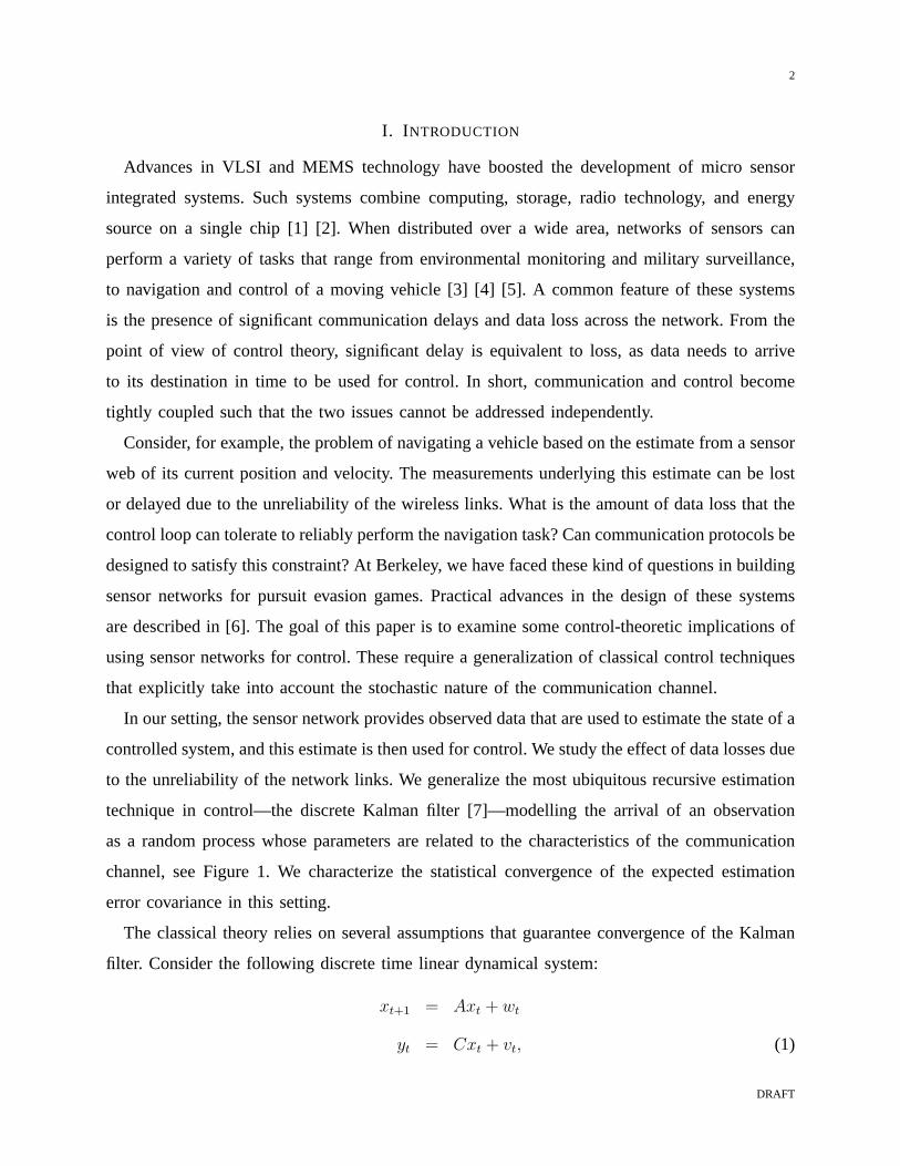
V. STATIC VERSUS OPTIMAL DYNAMIC KALMAN GAIN

In this section we compare the performance of filtering with static and dynamic gains for

a scalar discrete system. For the static estimator we follow the jump linear system approach

of [14]. The scalar static estimator case has been also worked out in [21].

Consider the dynamic state estimator

xdt+1 = Axd

t + γtKdt (yt − yt)

Kdt = APtC

′(CPtC′ + R)−1

Pt+1 = APtA′ + Q− γtAPtC

′(CPtC′ + R)−1CPtA

′ (24)

where the Kalman gainKdt is time-varying. Also consider the static state estimator

xst+1 = Axd

t + γtKs(yt − yt) (25)

where the estimator gainKs is constant. If no data arrives, i.e.γt = 0, both estimators simply

propagate the state estimate of the previous time-step.

The performance of the dynamic state estimator (24) has been analyzed in the previous

sections. The performance of static state estimator (25) can be readily obtained using jump

linear system theory [13] [14]. To do so, let us consider the estimator errorest+1

∆= xt+1 − xs

t+1.

Substituting Equations (1) forxt+1 and (25) forxst+1, we obtain the dynamics of the estimation

error:

est+1 = (A− γtKsC)es

t + vt + γtKswt. (26)

Using the same notation of Chapter 6 in Nilsson [14], where he considers the general system:

zk+1 = Φ(rk)zk + Γ(rk)ek

the system (26) can be seen as jump linear system switching between two statesrk ∈ {1, 2}given by:

Φ(1) = A−KsC Γ(1) = [1 Ks]

Φ(2) = A Γ(2) = [1 0]

DRAFT

16

where the noise covarianceE[eke′k] = Re, the transition probability matrixQπ and the steady

state probability distributionπ∞ are given by:

Re =

Q 0

0 R

Qπ =

λ 1− λ

λ 1− λ

π∞ =

[λ 1− λ

]

Following the methodology proposed in Nilsson [14], it is possible to show that the system

above is mean square stable, i.e.,limt→∞ E[(est)′es

t ] = 0 if and only if the transition probability

is

λ < λs =1

1− (1− KsC

A

)2

(1− 1

A2

). (27)

If the system is mean square stable, the steady state error covarianceP s∞ = limt→∞ E[es

t(est)′] is

given by:

P s∞ =

Q + K2s R

1− λ(A−KsC)2 − (1− λ)A2. (28)

Calculations to obtain Equations (27) and (28) are tedious but straightforward, therefore they

are omitted.

It is immediately evident that the transition probabilityλs of the estimator (25) using a static

gain is always greater than the transition probabilityλc of the estimator (24) which uses a

dynamic gain, in fact

λs = λc1

1− (1− KsC

A

)2

with equality only in the case whenKs = AC

. A natural choice for the estimator gainKs is

the steady state Kalman gain for the closed loop system (r = 1), which is always different

from AC

. Figure 6 shows the steady state error covariance for the scalar system considered in

the previous section, whereA = −1.5, C = 1, Q = 1, R = 2.5. The steady state Kalman gain

for this system isKSSKalman = −0.70, and the gain for largest mean square stability range is

Ks = AC

= −1.25. The figure also displays the upper bound of the state error covarianceV for

the dynamic estimator (24) that can be computed as indicated in Theorem 6. The steady state

error covariance of the static predictor for the two different gains is always greater than our

upper boundV . This is not surprising, since the dynamic estimator is optimal over all possible

estimators as shown in Section II. It is interesting to note that the static predictor with steady

state Kalman gain is close to the upper bound of the optimal predictor for arrival probability

DRAFT

17

0 0.1 0.2 0.3 0.4 0.5 0.6 0.7 0.8 0.9 10

5

10

15

20

25

30

λ

Sta

te E

rror

Cov

aria

nce

P

VK

s = K

SSKalmanK

s = A/C

λc

λs

Fig. 6. Error covariance boundV for dynamic predictor obtained from our theory and steady state error covariance for two

static predictors obtained from JLS theory using a steady state Kalman gain and maximum stability margin gain

close to unity, while the static predictor giving the largest stability margin approaches the optimal

predictor asymptotically for arrival probability close to the critical arrival probability.

From this example, it seems that the upper bound for the dynamic estimatorV gives an

estimate of the minimum steady state covariance that can be achieved with a static estimator for

any given arrival probability if the static gainKs is chosen optimally. Then the MARE could

be used to find the minimum steady state covariance and then the corresponding steady state

modified Kalman gain, thus providing an useful tool for optimal static estimator design. Future

work will explore this possibility.

VI. CONCLUSIONS

In this paper we have presented an analysis of Kalman filtering in the setting of intermittent

observations. We have shown how the expected estimation error covariance depends on the

tradeoff between loss probability and the system dynamics. Such a result is useful to the system

designer who must assess the relationship between the dynamics of the system whose state is

to be estimated and the reliability of the communication channel through which that system is

measured.

DRAFT

18

Our motivating application is a distributed sensor network that collects observations and sends

them to one or more central units that are responsible for estimation and control. For example,

in a pursuit evasion game in which mobile pursuers perform their control actions based on the

current estimate of the positions of both pursuers and evaders, the sensing capability of each

pursuer is generally limited, and an embedded sensor network is essential for providing a larger

overall view of the terrain. The results that we have presented here can aid the designer of the

sensor network in the choice of the number and disposition of the sensors.

This application also suggests a number of interesting directions for further work. For example,

although we have assumed independent Bernoulli probabilities for the observation events, in the

sensor network there will generally be temporal and spatial sources of variability that lead to

correlations among these events. While it is possible to compute posterior state estimates in such

a setting, it would be of interest to see if a priori bounds of the kind that we have obtained here

can be obtained in this case. Similarly, in many situations there may be correlations between

the states and the observation events; for example, such correlations will arise in the pursuit

evasion game when the evaders move near the boundaries of the sensor network. Finally, the

sensor network setting also suggests the use of smoothing algorithms in addition to the filtering

algorithms that have been our focus here. In particular, we may be willing to tolerate a small

amount of additional delay to wait for the arrival of a sensor measurement, if that measurement

is expected to provide a significant reduction in uncertainty. Thus we would expect that the

tradeoff that we have studied here between loss probability and the system dynamics should

also be modulated in interesting ways by the delay due to smoothing.

As another motoviation for considering more complex models that remove the assumption that

the arrivals are independent Bernoulli, one can imagine situations where some of the sensing is

done locally and therefore measurements are available at all sampling times, while measurements

taken at distant locations are available at irregular intervals. This would imply different dropping

rates for different channels.

VII. A PPENDIX A

In order to give complete proofs of our main theorems, we need to prove some preliminary

lemmas. The first lemma displays some useful properties of the MARE.

DRAFT

19

Lemma 1. Let the operator

φ(K, X) = (1− λ)(AXA′ + Q) + λ(FXF ′ + V ) (29)

whereF = A + KC, V = Q + KRK ′. AssumeX ∈ S = {S ∈ Rn×n|S ≥ 0}, R > 0, Q ≥ 0,

and (A,Q12 ) is controllable. Then the following facts are true:

(a) With KX = −AXC ′ (CXC ′ + R)−1, gλ(X) = φ(KX , X)

(b) gλ(X) = minK φ(K, X) ≤ φ(K, X)∀K(c) If X ≤ Y , thengλ(X) ≤ gλ(Y )

(d) If λ1 ≤ λ2 thengλ1(X) ≥ gλ2(X)

(e) If α ∈ [0, 1], thengλ(αX + (1− α)Y ) ≥ αgλ(X) + (1− α)gλ(Y )

(f) gλ(X) ≥ (1− λ)AXA′ + Q

(g) If X ≥ gλ(X), thenX > 0

(h) If X is a random variable, then(1− λ)AE[X]A′ + Q ≤ E[gλ(X)] ≤ gλ(E[X])

Proof: (a) DefineFX = A + KXC, and observe that

FXXC ′ + KXR = (A + KXC)XC ′ + KXR = AXC ′ + KX(CXC ′ + R) = 0.

Next, we have

gλ(X) = (1− λ)(AXA′ + Q) + λ(AXA′ + Q− AXC ′ (CXC ′ + R)−1

CXA′)

= (1− λ)(AXA′ + Q) + λ(AXA′ + Q + KXCXA′)

= (1− λ)(AXA′ + Q) + λ(FXXA′ + Q)

= (1− λ)(AXA′ + Q) + λ(FXXA′ + Q) + (FXXC ′ + KXR)K ′

= φ(KX , X)

(b) Let ψ(K, X) = (A + KC)X(A + KC)′ + KRK ′ + Q. Note that

argminKφ(K,X) = argminKFXF ′ + V = argminKψ(X, K).

SinceX,R ≥ 0, φ(K, X) is quadratic and convex in the variableK, therefore the minimizer

can be found by solving∂ψ(K,X)∂K

= 0, which gives:

2(A + KC)XC ′ + 2KR = 0 =⇒ K = −AXC ′ (CXC ′ + R)−1

.

Since the minimizer corresponds toKX defined above, the fact follows from fact (1).

DRAFT

20

(c) Note thatφ(K,X) is affine inX. SupposeX ≤ Y . Then

gλ(X) = φ(KX , X) ≤ φ(KY , X) ≤ φ(KY , Y ) = gλ(Y ).

This completes the proof.

(d) Note thatAXC ′(CXC ′ + R)−1CXA ≥ 0. Then

gλ1(X) = AXA′ + Q− λ1 AXC ′(CXC ′ + R)−1CXA

≥ AXA′ + Q− λ2 AXC ′(CXC ′ + R)−1CXA = gλ2(X)

(e) Let Z = αX + (1− α)Y whereα ∈ [0, 1]. Then we have

gλ(Z) = φ(KZ , Z)

= α(A + KZ C)X(A + KZ C)′ + (1− α)(A + KZ C)Y (A + KZ C)′+

+(α + 1− α)(KZ R K ′Z + Q)

= αφ(KZ , X) + (1− α)φ(KZ , Y )

≥ αφ(KX , X) + (1− α)φ(KY , Y )

= αgλ(X) + (1− α)gλ(Y ).

(30)

(f) Note thatFXXF ′X ≥ 0 andKRK ′ ≥ 0 for all K andX. Then

gλ1(X) = φ(KX , X) = (1− λ)(AXA′ + Q) + λ(FXXF ′X + KXRK ′

X + Q)

≥ (1− λ)(AXA′ + Q) + λQ = (1− λ)AXA′ + Q.

(g) From fact (f) follows thatX ≥ gλ1(X) ≥ (1 − λ)AXA′ + Q. Let X such thatX =

(1− λ)AXA′ + Q. SuchX must clearly exist. ThereforeX − X ≥ (1− λ)A(X − X)A′ ≥ 0.

Moreover the matrixX solves the Lyapunov EquationX = AXA′ + Q whereA =√

1− λA.

Since(A, Q12 ) is detectable, it follows thatX > 0 and soX > 0, which proves the fact.

(h) Using fact (f) and linearity of expectation we have

E[gλ(X)] ≥ E[(1− λ)AXA′ + Q] = (1− λ)AE[X]A′ + Q,

fact (e) implies that the operatorgλ() is concave, therefore by Jensen’s Inequality we have

E[gλ(X)] ≤ gλ(E[X]).

DRAFT

21

Lemma 2. Let Xt+1 = h(Xt) andYt+1 = h(Yt). If h(X) is a monotonically increasing function

then:

X1 ≥ X0 ⇒ Xt+1 ≥ Xt, ∀t ≥ 0

X1 ≤ X0 ⇒ Xt+1 ≤ Xt, ∀t ≥ 0

X0 ≤ Y0 ⇒ Xt ≤ Yt, ∀t ≥ 0

Proof: This lemma can be readily proved by induction. It is true fort = 0, sinceX1 ≥ X0

by definition. Now assume thatXt+1 ≥ Xt, thenXt+2 = h(Xt+1) ≥ h(Xt+1) = Xt+1 because

of monotonicity ofh(·). The proof for the other two cases is analogous.

It is important to note that while in the scalar caseX ∈ R eitherh(X) ≤ X or h(X) ≥ X;

in the matrix caseX ∈ Rn×n, it is not generally true that eitherh(X) ≥ X or h(X) ≤ X.

This is the source of the major technical difficulty for the proof of convergence of sequences in

higher dimensions. In this case convergence of a sequence{Xt}∞0 is obtained by finding two

other sequences,{Yt}∞0 , {Zt}∞0 that boundXt, i.e., Yt ≤ Xt ≤ Zt,∀t, and then by showing that

these two sequences converge to the same point.

The next two lemmas show that when the MARE has a solutionP , this solution is also stable,

i.e., every sequence based on the difference Riccati equationPt+1 = gλ(Pt) converges toP for

all initial positive semidefinite conditionsP ≥ 0.

Lemma 3. Define the linear operator

L(Y ) = (1− λ)(AY A′) + λ(FY F ′)

Suppose there existsY > 0 such thatY > L(Y ).

(a) For all W ≥ 0,

limk→∞

Lk(W ) = 0

(b) Let U ≥ 0 and consider the linear system

Yk+1 = L(Yk) + U initialized at Y0.

Then, the sequenceYk is bounded.

Proof: (a) First observe that0 ≤ L(Y ) for all 0 ≤ Y . Also, X ≤ Y impliesL(X) ≤ L(Y ).

Choose0 ≤ r < 1 such thatL(Y ) < rY . Choose0 ≤ m such thatW ≤ mY . Then,

0 ≤ Lk(W ) ≤ mLk(Y ) < mrkY

DRAFT

22

The assertion follows when we take the limitr →∞, on noticing that0 ≤ r < 1.

(b) The solution of the linear iteration is

Yk = Lk(Y0) +k−1∑t=0

Lt(U)

≤(

mY0rk +

k−1∑t=0

mUrt

)Y

≤(

mY0rk +

mU

1− r

)Y

≤(

mY0 +mU

1− r

)Y

proving the claim.

Lemma 4. Consider the operatorφ(K, X) defined in Equation (29). Suppose there exists a

matrix K and a positive definite matrixP such that

P > 0 and P > φ(K, P ).

Then, for anyP0, the sequencePt = gtλ(P0) is bounded, i.e. there existsMP0 ≥ 0 dependent of

P0 such that

Pt ≤ M for all t.

Proof: First define the matricesF = A + KC and consider the linear operator

L(Y ) = (1− λ)(AY A′) + λ(FY F′)

Observe that

P > φ(K, P ) = L(P ) + Q + λKRK′ ≥ L(P ).

Thus,L meets the condition of Lemma 3. Finally, using fact (b) in Lemma 1 we have

Pt+1 = gλ(Pt) ≤ φ(K, Pt) = LPt + Q + λKRK′= L(Pt) + U.

SinceU = λKRK′+ Q ≥ 0, using Lemma 3, we conclude that the sequencePt is bounded.

We are now ready to give proofs for Theorems 1-4.

DRAFT

23

A. Proof of Theorem 1

(a) We first show that the modified Riccati difference equation initialized atQ0 = 0 converges.

Let Qk = gkλ(0). Note that0 = Q0 ≤ Q1. It follows from Lemma 1(c) that

Q1 = gλ(Q0) ≤ gλ(Q1) = Q2.

A simple inductive argument establishes that

0 = Q0 ≤ Q1 ≤ Q2 ≤ · · · ≤ MQ0 .

Here, we have used Lemma 4 to bound the trajectory. We now have a monotone non-decreasing

sequence of matrices bounded above. It is a simple matter to show that the sequence converges,

i.e.

limk→∞

Qk = P .

Also, we see thatP is a fixed point of the modified Riccati iteration:

P = gλ(P ),

which establishes that it isa positive semidefinite solution of the MARE.

Next, we show that the Riccati iteration initialized atR0 ≥ P also converges, and to the same

limit P . First define the matrices

K = −APC ′ (CPC ′ + R)−1

, F = A + KC

and consider the linear operator

L(Y ) = (1− λ)(AY A′) + λ(FY F′).

Observe that

P = gλ(P ) = L(P ) + Q + KRK′> L(P ).

Thus,L meets the condition of Lemma 3. Consequently, for allY ≥ 0,

limk→∞

Lk(Y ) = 0.

Now supposeR0 ≥ P . Then,

R1 = gλ(R0) ≥ gλ(P ) = P .

DRAFT

24

A simple inductive argument establishes that

Rk ≥ P for all k.

Observe that

0 ≤ (Rk+1 − P ) = gλ(Rk)− gλ(P )

= φ(KRk, Rk)− φ(KP , P )

≤ φ(KP , Rk)− φ(KP , P )

= (1− λ)A(Rk − P )A′ + λFP (Rk − P )F ′P

= L(Rk − P ).

Then,0 ≤ limk→∞(Rk+1 − P ) ≤ 0, proving the claim.

We now establish that the Riccati iteration converges toP for all initial conditionsP0 ≥ 0.

Define Q0 = 0 and R0 = P0 + P . Consider three Riccati iterations, initialized atQ0, P0, and

R0. Note that

Q0 ≤ P0 ≤ R0.

It then follows from Lemma 2 that

Qk ≤ Pk ≤ Rk for all k.

We have already established that the Riccati equationsPk and Rk converge toP . As a result,

we have

P = limk→∞

Pk ≤ limk→∞

Qk ≤ limk→∞

Rk = P ,

proving the claim.

(b) Finally, we establish that the MARE has a unique positive semidefinite solution. To this

end, considerP = gλ(P ) and the Riccati iteration initialized atP0 = P . This yields the constant

sequence

P , P , · · ·

However, we have shown that every Riccati iteration converges toP . ThusP = P .

DRAFT

25

B. Proof of Theorem 2

First we note that the two cases expressed by the theorem are indeed possible. Ifλ = 1 the

modified Riccati difference equation reduces to the standard Riccati difference equation, which

is known to converge to a fixed point, under the theorem’s hypotheses. Hence, the covariance

matrix is always bounded in this case, for any initial conditionP0 ≥ 0. If λ = 0 then we reduce

to open loop prediction, and if the matrixA is unstable, then the covariance matrix diverges

for some initial conditionP0 ≥ 0. Next, we show the existence of a single point of transition

between the two cases. Fix a0 < λ1 ≤ 1 such thatEλ1 [Pt] is bounded for any initial condition

P0 ≥ 0. Then, for anyλ2 ≥ λ1 Eλ2 [Pt] is also bounded for allP0 ≥ 0. In fact we have

Eλ1 [Pt+1] = Eλ1 [APtA′ + Q− γt+1APtC

′(CPtC′ + R)−1CPtA]

= E[APtA′ + Q− λ1APtC

′(CPtC′ + R)−1CPtA]

= E[gλ1(Pt)]

≥ E[gλ2(Pt)]

= Eλ2 [Pt+1],

where we exploited fact (d) of Lemma 1 to write the above inequality . We can now choose

λc = {inf λ∗ : λ > λ∗ ⇒ Eλ[Pt]is bounded, for allP0 ≥ 0},

completing the proof.

C. Proof of Theorem 3

Define the Lyapunov operatorm(X) = AXA′+Q whereA =√

1− λA. If (A,Q12 ) is control-

lable, also(A, Q12 ) is controllable. Therefore, it is well known thatS = m(S) has a unique strictly

positive definite solutionS > 0 if and only if maxi |σi(A)| < 1, i.e.√

1− λ maxi |σi(A)| < 1,

from which follows λ = 1 − 1α2 . If maxi |σi(A)| ≥ 1 it is also a well known fact that there

is no positive semidefinite fixed point to the Lyapunov equationS = m(S), since(A, Q12 ) is

controllable.

Let us consider the difference equationSt+1 = m(St), S0 = 0. It is clear thatS0 = 0 ≤Q = S1. Since the operatorm() is monotonic increasing, by Lemma 2 it follows that the

sequence{St}∞0 is monotonically increasing, i.e.St+1 ≥ St for all t. If λ < λ this sequence

DRAFT

26

does not converge to a finite matrixS, otherwise by continuity of the operatorm we would

haveS = m(S), which is not possible. Since it is easy to show that a monotonically increasing

sequenceSt that does not converge is also unbounded, then we have

limt→∞

St = ∞.

Let us consider now the mean covariance matrixE[Pt] initialized at E[P0] ≥ 0. Clearly

0 = S0 ≤ E[P0]. Moreover it is also true

St ≤ E[Pt] =⇒ St+1 = (1− λ)AStA′ + Q ≤ (1− λ)AE[Pt]A

′ + Q ≤ E[gλ(Pt)] = E[Pt+1],

where we used fact (h) from Lemma 1. By induction, it is easy to show that

St ≤ E[Pt] ∀t, ∀E[P0] ≥ 0 =⇒ limt→∞

E[Pt] ≥ limt→∞

St = ∞.

This implies that for any initial conditionE[Pt] is unbounded for anyλ < λ, thereforeλ ≤ λc,

which proves the first part of the Theorem.

Now consider the sequenceVt+1 = gλ(Vt), V0 = E[P0] ≥ 0. Clearly

E[Pt] ≤ Vt =⇒ E[Pt+1] = E[gλ(Pt)] ≤ gλ(E[Pt]) ≤ [gλ(Vt)] = Vt+1,

where we used facts (c) and (h) from Lemma 1. Then a simple induction argument shows

that Vt ≥ E[Pt] for all t. Let us consider the caseλ > λ, therefore there existsX such that

X ≥ gλ(X). By Lemma 1(g)X > 0, therefore all hypotheses of Lemma 3 are satisfied, which

implies that

E[Pt] ≤ Vt ≤ MV0 ∀t.

This shows thatλc ≤ λ and concludes the proof of the Theorem.

D. Proof of Theorem 4

Let consider the sequencesSt+1 = (1 − λ)AStA′ + Q, S0 = 0 and Vt+1 = gλ(Vt), V0 =

E[P0] ≥ 0. Using the same induction arguments in Theorem 3 it is easy to show that

St ≤ E[Pt] ≤ Vt ∀t.

From Theorem 1 follows thatlimt→∞ Vt = V , whereV = gλV . As shown before the sequenceSt

is monotonically increasing. Also it is bounded sinceSt ≤ Vt ≤ M . Thereforelimt→∞ St = S,

and by continuityS = (1 − λ)ASA′ + Q, which is a Lyapunov equation. Since√

1− λA is

DRAFT

27

stable and(A,Q12 ) is controllable, then the solution of the Lyapunov equation is strictly positive

definite, i.e.S > 0. Adding all the results together we get

0 < S = limt→∞

St ≤ limt→∞

E[Pt] ≤ limt→∞

Vt = V ,

which concludes the proof.

DRAFT

28

REFERENCES

[1] Smart dust project home page. http://robotics.eecs.berkeley.edu/ pister/SmartDust/.

[2] NEST project at Berkeley home page. http://webs.cs.berkeley.edu/nest-index.html.

[3] Seismic sensor research at berkeley, home page. http://www.berkeley.edu/news/media/releases /2001/12/13snsor.html.

[4] P. Varaiya, “Smart cars on smart roads: Problems of control,”IEEE Transactions on Automatic Control, vol. 38(2), February

1993.

[5] J. Lygeros, D. N. Godbole, and S. S. Sastry, “Verified hybrid controllers for automated vehicles,”IEEE Transactions on

Automatic Control, vol. 43(4), 1998.

[6] B. Sinopoli, C. Sharp, S. Schaffert, L. Schenato, and S. Sastry, “Distributed control applications within sensor networks,”

IEEE Proceedings Special Issue on Distributed Sensor Networks, November 2003.

[7] R. E. Kalman, “A new approach to linear filtering and prediction problems,”Transactions of the ASME - Journal of Basic

Engineering on Automatic Control, vol. 82(D), pp. 35–45, 1960.

[8] P. S. Maybeck,Stochastic models, estimation, and control, ser. Mathematics in Science and Engineering, 1979, vol. 141.

[9] M. Micheli and M. I. Jordan, “Random sampling of a continiuous-time stochastic dynamical system,” inProceedings of

15th International Symposium on the Mathematical Theory of Networks and Systems (MTNS), University of Notre Dame,

South Bend, Indiana, August 2002.

[10] M. Micheli, “Random sampling of a continuous-time stochastic dynamical system: Analysis, state estimation, applications,”

Master’s Thesis, University of California at Berkeley, Deparment of Electrical Engineering, 2001.

[11] M. Athans, R. Ku, and S. B. Gershwin, “The uncertainty threshold principle, some fundamental limitations of optimal

decision making under dynamic uncertainty,”IEEE Transactions on Automatic Control, vol. 22(3), pp. 491–495, June

1977.

[12] R. Ku and M. Athans, “Further results on the uncertainty threshold principle,”IEEE Transactions on Automatic Control,

vol. 22(5), pp. 491–495, October 1977.

[13] M. Mariton, Jump Linear Systems in Automatic Control. Marcel Dekker, 1990.

[14] J. Nilsson, “Real-time control systems with delays,” Ph.D. dissertation, Department of Automatic Control, Lund Institute

of Technology, 1998.

[15] J. Nilsson, B. Bernhardsson, and B. Wittenmark, “Stochastic analysis and control of real-time systems with random time

delays.” [Online]. Available: citeseer.nj.nec.com/101333.html

[16] Q. Ling and M. Lemmon, “Soft real-time scheduling of networked control systems with dropouts governed by a markov

chain,” in American Control Conference, June 2003, denver, CO.

[17] T. Fortmann, Y. Bar-Shalom, M. Scheffe, and S. Gelfand, “Detection thresholds for tracking in clutter-a connection between

estimation and signal processing,”IEEE Transactions on Automatic Control, vol. AC-30, no. 3, pp. 221–228, March 1985.

[18] N. M. Dempster, A. Laird, and D. B. Rubin, “Maximum likelihood from incomplete data via the EM algorithm,”Journal

of the Royal Statistical Society B, vol. 39, pp. 185–197, 1977.

[19] R. H. Shumway and D. S. Stoffer,Time Series Analysis and Its Applications. Springer Verlag, March 2000.

[20] S. Lauritzen,Graphical Models. Clarendon Press, 1996.

[21] C. N. Hadjicostis and R. Touri, “Feedback control utilizing packet dropping network links,” inProceedings of the 41st

IEEE Conference on Decision and Control, Las Vegas, NV, Dec 2002, invited.

DRAFT