Embed Size (px)
Citation preview

INDUSTRIAL POLICIES IN PRODUCTION NETWORKS*
Ernest Liu†
First Draft: October 2016
This Draft: October 2017
Abstract
Many developing countries adopt industrial policies that push resources towards selected
economic sectors. How should countries choose which sectors to promote? I answer this ques-
tion by characterizing optimal industrial policy in production networks embedded with market
imperfections. My key finding is that effects of market imperfections accumulate through
backward demand linkages, thereby generating aggregate sales distortions that are largest in
the most upstream sectors. The distortion in sectoral sales is a sufficient statistic for the ratio
between social and private marginal product of sectoral inputs; therefore, there is an incentive
for a well-meaning government to subsidize upstream sectors. My sufficient statistic predicts
the sectors targeted by government interventions in South Korea in the 1970s and in modern-
day China.
JEL Codes: C67, O11, O25, O47
Word Count: 12,758
*Previous circulated under title “Industrial Policies and Economic Development”. I am indebted to Daron Ace-moglu and Abhijit Banerjee for their guidance and support throughout this project. I thank Marios Angeletos, DavidAtkin, Sandeep Baliga, David Baqaee, Arnaud Costinot, Esther Duflo, Yan Ji, Nobu Kiyotaki, Pete Klenow, DavidLaibson, Nathaniel Lane, Pooya Molavi, Ben Moll, Dilip Mookherjee, Dani Rodrik, Gerard Roland, Alp Simsek,Andrei Shleifer, Ludwig Straub, Tavneet Suri, Linh Tô, Pengfei Wang, Shang-Jin Wei, David Weil, Ivan Werning,Heiwai Tang, Rob Townsend, Venky Venkateswaran, Daniel Xu, Hanzhe Zhang, Xiaodong Zhu, Fabrizio Zilibotti,and especially Chad Jones, Daniel Green, Atif Mian, Nancy Qian, Jesse Shapiro, and Aleh Tsyvinski, as well as semi-nar participants at MIT, Harvard, BU, Rochester, HKUST, JHU-SAIS, Brown, Kellogg MEDS, NBER-China meeting,Stanford SITE, and Bank of Canada-University of Toronto conference for helpful comments.
†Princeton University. Email: [email protected]. Address: 214 Julis Rabinowitz Bldg, Princeton NJ 08544.
1

1 Introduction
One of the oldest problems in economics is understanding how industrial policies can facilitateeconomic development. What is industrial policy? Broadly speaking, it is purposeful governmentintervention to selectively promote specific economic sectors. Industrial policies have been promi-nently adopted in many currently and formerly developing economies: Japan from the 1950s to1970s, South Korea and Taiwan from the 1960s to 1980s, and modern-day China.
By their nature, these policies seek to affect the aggregate economy by targeting a few sectors;hence, cross-sector linkages are important considerations (Hirschman 1958). Loose economic rea-soning suggests that it may be advantageous to subsidize or promote the development of sectorsthought to serve as backbones of the economy—natural resource production, iron and steel indus-tries, etc. Indeed, this has often been the strategy taken by countries implementing such policies.Policy documents from these interventionist governments often explicitly state “network linkages”as a criterion for choosing sectors to support.1
Despite their widespread use and loosely supporting intuition, economists have only a verylimited formal understanding of the forms these policies should take. In this paper, I build onthe production networks literature and provide the first formal analysis of industrial policy in thepresence of cross-sector linkages and market imperfections. My key finding is that the effects ofmarket imperfections accumulate through what I call “backward demand linkages”, causing certainsectors to become the “sink” of distortions, thereby creating an incentive for well-meaning gov-ernments to subsidize them. The sectors in which distortions accumulate are typically designatedin the networks literature as “upstream,” meaning they supply to many other sectors and use fewinputs from other sectors. In the data, this notion corresponds with the same sectors policymakersseem to view as important targets for intervention.
To develop my results, I start with a canonical model of production network and embed in it ageneric formulation of market imperfections, which can be microfounded by a variety of under-lying frictions. Market imperfections distort the use of sectoral inputs, resulting in their marginalproducts exceeding marginal costs. Such distortions accumulate over the production network andaggregate to alter productive sectors’ equilibrium size away from their optimal size. I show thatthis aggregate distortion in the size of a sector is a sufficient statistic for the ratio between socialand private marginal revenue products in that sector. I term the sufficient statistic “distortion cen-trality”—it is one scalar per sector and is defined as the ratio between sectoral influence, which
1See Li and Yu (1982), Kuo (1983), and Yang (1993) for Taiwan; Kim (1997) for Korea; and State DevelopmentPlanning Commission of China (1995) for China.
2
captures sectoral size under optimal production, and sectoral sales, which is the sectoral size inequilibrium.
In the economy, the first welfare theorem holds in the absence of market imperfections; there-fore, the first-best equilibrium can be trivially restored if all imperfections can be removed. Onthe other hand, when market imperfections cannot be directly corrected, there is room for a well-meaning government to interfere with market allocations, and distortion centrality guides opti-mal sectoral interventions. Specifically, I show that, holding within-sector distortions constant, abenevolent government should provide the first dollar of production subsidies to sectors with thehighest distortion centrality. My results apply to marginal tax instruments that directly or indi-rectly expand sectoral input use; such instruments include subsidies to value-added and intermedi-ate inputs, subsidies to sales, and transfers of working capital if market imperfections arise due tofinancial constraints. Furthermore, if production functions are Cobb-Douglas, distortion centralityis informative for not only marginal but also constrained-optimal subsidies to value-added input.
Perhaps surprisingly, sectors with the highest distortion centrality are not necessarily the mostdistorted sectors; instead, they tend to be upstream ones that supply to many distorted downstreamsectors. This is because market imperfections accumulate through backward demand linkagesover the production network. When a sector is distorted, the producer purchases less-than-optimalamounts of inputs from its suppliers, thereby depressing the sales of these upstream suppliers,which in turn purchase less from their own input suppliers. The effect keeps transmitting upstreamthrough intermediate demand, and, as a result, the most upstream sector becomes the “sink” of alldistortions in the economy and thus has the highest distortion centrality.
In a general production network, distortion centrality depends on market imperfections in everysector of the economy, the estimation of which is a formidable task. Indeed, a major criticism ofindustrial policies is that it is impossible for governments to identify the relevant sectors that aresubject to market imperfections; simply put, “government cannot pick winners” (Rodrik 2008).Yet, precisely because distortions backwardly accumulate, I show that if the equilibrium input-output structure exhibits log-supermodularity—so that relatively upstream sectors use upstreaminputs more intensively—then the rank ordering of sectoral distortion centrality is insensitive to thedistribution of underlying market imperfections. This result suggests that it is unnecessary to pre-cisely estimate sectoral imperfections in order to conduct welfare-improving policy interventions.In the absence of an exact intervention that directly removes market imperfections—due to eitherpolicy infeasibility or informational constraints—the second-best policy in a log-supermodularnetwork is always to subsidize the upstream sectors, to which all distortions eventually propagate,no matter where they originate in the network.
3

My analysis calls for a re-evaluation of industrial policies in developing countries. Many criticsof industrial policies draw on insights from the misallocation literature popularized by Hsieh andKlenow (2009) and Restuccia and Rogerson (2008), a line of work that quantitatively evaluatesthe loss in aggregate TFP due to firms failing to equalize the marginal revenue products of inputs.Pointing to the logical inevitability that sector-based policies generate “misallocation across sec-tors” and the empirical evidence that firms in the subsidized sectors tend to have lower marginalrevenue products, critics conclude that sectoral interventions must lower welfare.2 My theoreticalresults challenge this logic. Whereas within-sector dispersion in private marginal revenue productsunambiguously lowers productive efficiency, as the misallocation literature suggests, my analysisshows that cross-sector dispersion in private marginal revenue products could enhance welfare.This is because in the presence of cross-sector linkages, social and private marginal revenue prod-ucts are not equal; in fact, I provide an example in section 5 in which the rank orderings of sectoralprivate and social marginal revenue products are reversed. Spending in upstream sectors tends tohave higher social return precisely because these sectors have high distortion centrality. In otherwords, to equate social marginal revenue products across sectors, the private marginal revenueproducts have to be lower in the upstream sectors in a distorted production network. My anal-ysis therefore provides a counterpoint to the prevailing view that selective interventions and theconsequent cross-sector misallocations must be a sign of inefficiency.
I apply my theoretical insights and empirically examine the input-output structures of SouthKorea during the 1970s and modern-day China, as these are two of the most salient economies withinterventionist governments that have actively implemented industrial policies. I show that theseeconomies’ input-output structures approximately exhibit log-supermodularity, and, as a result,distortion centrality is insensitive to the distribution of underlying market imperfections. Further,I find that distortion centrality predicts the sectors targeted by government interventions in both ofthese economies. The sectors South Korea promoted in the 1970s have, on average, significantlyhigher distortion centrality. In modern-day China, privately-owned firms in sectors with higherdistortion centrality have significantly better access to loans at more favorable interest rates, andthese sectors also tend to have more state-owned enterprises, to which the government directlyextends subsidies and credit in order to expand sectoral production. To be clear, these correlationsby no means suggest that policies adopted by these economies were optimal: my theory abstractsaway from practical aspects of policy implementation as well as the various political economyfactors that affect policy choices in these economies (Krueger 1990). Nevertheless, my resultssuggest that there are aspects of Korean and Chinese industrial strategy that appear to be motivatedby a desire to subsidize sectors that create positive network effects.
2For example, see Ruiz (2003), Nabli et al. (2006), Chung (2007), Sun (2009), Dabla-Norris et al. (2015), Calli-garis et al. (2016), Gebresilasse (2016), and Leal (2015, 2017).
4

Literature Review The literature on industrial policies dates back to at least the seminal con-tributions by Rosenstein-Rodan (1943) and Hirschman (1958).3 Recent contributions to this lit-erature include Rodrik (2004, 2008), Robinson (2010), and Cheremukhin et al. (2017a, 2017b),among many others. My paper revisits Hirschman’s thesis on the importance of cross-sector input-output linkages for development policies by formally analyzing the effect of government interven-tions in production networks with market imperfections. In a recent paper, Lane (2017) empiricallystudies South Korea’s industrial policies during the 1970s and finds evidence for pecuniary exter-nalities, i.e. that sectors downstream of the promoted ones experienced positive spillovers fromthe industrial policy program. My theoretical analysis shows that the general equilibrium effectsof such pecuniary externalities can be succinctly characterized in order to design optimal interven-tions, and I show that my characterization predicts the sectors promoted in both historical SouthKorea and modern-day China.
Methodologically, my paper builds on the production networks literature. The paper to whichmy work most closely relates is Jones (2013), who embeds generic distortions into a Cobb-Douglasproduction economy with cross-sector linkages and studies the implications of distortions for ag-gregate output. The presence of distortions in Jones (2013) implies that sectoral influence is decou-pled from sales. Following Jones (2013), there is a burgeoning literature that investigates the ef-fects of market imperfections on aggregate output, including Bartelme and Gorodnichenko (2015),Altinoglu (2015), Bigio and La’O (2016), Baqaee (2017), Boehm (2017), and Grassi (2017).Caliendo et al. (2017) develop methodologies to identify sectoral distortions in production net-works.
I make several contributions to this literature. First, I show that in a distorted production net-work, distortion centrality—the wedge between sectoral influence and sales—captures the ratiobetween social and private marginal revenue product in a sector. As a result, distortion centralityguides the optimal marginal interventions that directly or indirectly shift the use of production in-puts. Second, I explicitly characterize how underlying market imperfections are aggregated intodistortion centrality. I show that imperfections accumulate through backward demand linkages;therefore, the upstream sectors become the “sink” of distortions and tend to have the highestdistortion centrality. Neither of these results relies on the strong Cobb-Douglas or the constantelasticity-of-substitution functional assumptions imposed by this literature.
My paper also relates to the large body of macro-development literature on the misallocationof resources, including Banerjee and Duflo (2005), Restuccia and Rogerson (2008), Hsieh andKlenow (2009), Banerjee and Moll (2010), Song et al. (2011), Buera et al. (2011), Midrigan
3Other key references in the vast literature on industrial policies include Chenery et al. (1986), Amsden (1989),Murphy et al. (1989), Krueger (1990), Wade (1990), Westphal (1990), Page (1994), and Woo-Cumings (2001).
5

and Xu (2014), and Rotemberg (2017) among many others. The literature’s central line of in-quiry addresses the implications of micro-level market imperfections on aggregate productivity.My paper draws on this literature but shifts the focus: I study misallocation across—rather thanwithin—sectors. I show that in the presence of input-output linkages, private and social marginalrevenue products no longer coincide. As a result, equating private marginal revenue productsacross sectors is no longer sufficient for constrained efficiency: social marginal revenue productscan still vary, and the aggregate productive efficiency can be improved if inputs are redirected tosectors with high distortion centrality.
The rest of the paper is organized as follows: Section 2 introduces a generic formulation ofmarket imperfections into a canonical model of production network. Section 3 characterizes thedistorted equilibrium. Section 4 introduces the distortion centrality measure and studies its im-plication for policy interventions. Section 5 characterizes how distortion centrality is shaped byunderlying market imperfections and network structure. Section 6 applies the model and em-pirically examines the input-output relationship in historical South Korea as well as modern-dayChina. Section 7 concludes.
2 A Production Network With Market Imperfections
2.1 Model
This section lays out my model, which strikes a balance between generality and tractability.To focus on the policy implications of market imperfections in a production network and obtainsharp characterizations, the model deliberately features simplistic factor supply and consumptiondecisions.
Economic Environment The economy has a production factor in fixed supply, L, which werefer to as “labor” but can be alternatively interpreted as a composite factor consisting of laborand other factor inputs. There is a representative consumer who has non-satiated preferences andconsumes a unique final good (with price normalized to one). There are S intermediate productionsectors,4 each producing a differentiated good that is used for both intermediate production andthe production of the unique final good. I will refer to the output of sector i as good i and to the S
goods altogether as “intermediate goods”.
4I use the terms “sector” and “industry” interchangeably.
6

The final good is produced competitively by combining intermediate goods under productionfunction
Y = F (Y1, · · · ,YS) , (1)
where Yi is the units of good i used for final production and Y is the aggregate output. I assumeF (·) is differentiable, has constant-returns-to-scale, and is strictly increasing and jointly concavein its arguments.
Each intermediate good i is produced by a constant returns to scale production technology
Qi = ziFi
(Li,
Mi j
j∈S
), (2)
where Li is the total labor employed in sector i and zi captures the Hicks-neutral sectoral pro-ductivity. The terms
Mi j
denote the amount of intermediate goods ( j’s) used by sector i asproduction inputs, and this dependence on intermediate goods captures the notion of productionlinkages across sectors.
Assumption 1. Production functions Fi and F are continuously differentiable and strictly concave.
Furthermore, Fi (0,Mi1, · · ·MiS) = 0 and ∂Fi(Li,Mi1,···MiS)∂Li
> 0 at all input levels. That is, every sector
needs labor to produce, and sectoral output is always strictly increasing in labor.
Market Imperfections And Distorted Equilibrium The economic setting described thus farfalls under the class of “generalized Leontief models” as defined by Arrow and Hahn (1971, pp.40). It is well known that the First Welfare Theorem holds in this environment, and the decen-tralized equilibrium would be efficient if each intermediate good is produced by a price-takingrepresentative firm. I introduce market imperfections into this economy by specifying that theallocations are “as if” chosen by a fictitious price-taking representative firm in each intermediatesector, with the fictitious firm facing input prices that are exogenously distorted upwards.
Specifically, let Pj denote the cost of purchasing good j. Market imperfections in sector i takethe form of exogenous distortions χL
i and
χi jS
j=1 such that equilibrium allocations are “as if”chosen by a price-taking and profit-maximizing representative firm, which faces a “shadow price”of(1+χL
i)
W for labor and Pj(1+χi j
)for input j ∈ S, with χL
i ,χi j ≥ 0.
Definition 1. Given distortions
χLiS
i=1 and
χi jS
i, j=1, a Distorted Equilibrium is the collection
of prices PiSi=1, wage rate W , sectoral allocations
Qi,Li,
Mi jS
j=1
S
i=1, production inputs for
the final good YiSi=1, and aggregate output Y such that
1. Prices and sectoral allocations solve the cost-minimization problem of the fictitious price-
7

taking sectoral producers:
Pi = Ci(W,
Pj)≡ min
`i,mi jSj=1
(∑j∈S
(1+χi j
)Pjmi j +
(χ
Li)
W`i
)(3)
s.t. ziFi
(`i,
mi jS
j=1
)≥ 1,
andLi = Qi · `∗i ,
Mi j = Qi ·m∗i j,
where`∗i ,
m∗i j
is the solution to the cost minimization problem;
2. Production inputs for the final good satisfy:
∂F (Y1, · · · ,YS)
∂Yi= Pi; (4)
3. Factor and intermediate goods markets clear:
Q j = Yj +S
∑i=1
Mi j, (5)
L =S
∑i=1
Li; (6)
4. The representative consumer spend labor income on the final good:
C =WL = Y −S
∑i=1
(∑j∈S
(1+χi j
)PjMi j +
(1+χ
Li)
WLi
). (7)
Discussion The definition of Distorted Equilibrium requires only that allocations are as-if chosenby a price-taking firm, and the definition is deliberately agnostic about both the actual marketstructure and the source of price distortions. My theoretical results in sections 3, 4, and 5 applyto any microfoundation that induces equilibrium prices and allocations that coincide with thisgeneric definition of Distorted Equilibrium. The next subsection provides microfoundations of theDistorted Equilibrium under various market imperfections and market structures.
Equation (7) specifies that payments associated with the market imperfections are not rebated
8

to the representative consumer, whose consumption C is equal to the value of total factor paymentsWL. Instead, the distortion payments correspond to deadweight losses in the economy, such asexcess entry or real costs incurred with pecuniary transactions across sectors, and are thereforesubtracted from the aggregate output. The specification also nests the interpretation that thesedistortion payments are made to agents other than the representative consumer. My theoreticalanalyses in sections 3 and 4 study the impact of various policy instruments on C, the aggregateconsumption of the representative consumer; hence, my results apply to both interpretations.
2.2 Microfoundations
To make discussions concrete, in this subsection I provide four different microfoundations forthe Distorted Equilibrium. Distortion payments are modeled as deadweight losses in all four cases.Readers who are more interested in directly seeing the main theoretical results can skip ahead tosection 3.
The first two microfoundations are based on financial frictions with deadweight losses generatedby, respectively, the excess entry of constrained firms and the monitoring cost for the repaymentof working capital. Market imperfections in the third microfoundation are based on monopolisticmarkups, and the fourth builds on Marshallian externalities. Although market imperfections inthese four microfoundations come from varying sources and productions are based on differentmarket structures, all four microfoundations induce equilibrium prices and allocations that coincidewith those in Definition 1.
Financial Frictions - Working Capital Constraints The first microfoundation is based on fi-nancial frictions. I assume each producer faces an exogenous working capital constraint on thepurchase of certain intermediate inputs Di ⊂ S, and the distortion χi j ≡ χi for all j ∈ Di in thiscase corresponds to either the shadow value on working capital or the Lagrange multiplier on theconstraint in sector i.
Specifically, intermediate production is modeled as a two-stage entry game. In the first stage, alarge measure of identical and atomistic potential entrants choose whether to set up a firm in anysector, paying a fixed cost κi (in units of the final good) if they decide to enter in sector i. In thesecond stage, firms in sector i produce the identical and perfectly substitutable good i according toa constant-returns-to-scale production function
qi = ziFi (`i,mi1, · · · ,miS) (8)
9

while taking prices as given and facing a working capital constraint
∑j∈Di
Pjmi j ≤ Γi, (9)
where Γi denotes the exogenous amount of working capital available to each firm in sector i. (Notethat I use lower-case letters to denote firm-level variables while, as before, the correspondingupper-case letters denote sectoral and aggregate variables.)
I now argue that the decentralized equilibrium in this environment has sectoral prices and al-locations that coincide with those in Definition 1. Each firm takes prices as given and maximizesvariable profit:
max`i,mi j
PiziFi(`i,
mi j)−W`i−∑
j∈SPjmi j subject to (9).
Let χi be the constraint’s Lagrange multiplier, which captures firms’ willingness to pay for addi-tional working capital. The term (1+χi) captures the ratio between marginal product and marginalcost of the constrained inputs. To pin down χi, an endogenous object, I note that the variable profitaccrued to each firm is πi = χiΓi. These positive profits in turn lead to excessive entry and dead-weight losses in equilibrium, with πi = κi as ensured by the free-entry condition. The Lagrangemultiplier χi is therefore equal to κi/Γi. The unconstrained inputs are not subject to distortionsaccording to this microfoundation.
The total sectoral output and inputs are equal to
Qi = Niqi, Li = Ni`i, Mi j = Nimi j. (10)
Since Fi (·) features constant-returns-to-scale, we can write
Qi = NiziFi(`i,
mi j)
= ziFi(Li,
Mi j)
. (11)
Sectoral allocations and prices therefore coincide with those in Definition 1, with χi j = κi/Γi forall j ∈ Di and χi j = 0 otherwise. The amount of final good used for consumption is equal to theaggregate output net of entry cost κiNi = χi ∑ j∈Di PjMi j, satisfying condition 7.
Under this microfoundation, inputs in Di require working capital to purchase, and these inputscan be thought of as capital goods (e.g. machinery, equipments, and computers) or services thatcan be subject to hold-up problems (such as outsourced R&D services), for which trade credit isdifficult to obtain and costs must be incurred upfront. The unconstrained inputs can be thought ofas material or commodity inputs—such as intermediate materials for the production of consumer
10

goods (e.g. textiles) and commoditized services—for which trade credit is more available (Fisman2001) such that the input cost can be paid after production.
Financial Frictions - Monitoring Costs The second and perhaps simplest microfoundation forthe Distorted Equilibrium assumes there is a representative firm in each intermediate sector withproduction technology specified in (2), and each firm i must borrow working capital in order tofinance the purchases of certain intermediate inputs j ∈ Di ⊂ S. There is a representative financialinstitution (lender) that extends working capital to intermediate producers and incurs a proportional(linear) expense χ in terms of the final good while doing so. The expense χ can be thought of asmonitoring costs that must be incurred to ensure working capital is repaid after production. Thelender behaves competitively and makes zero profit, charging a flat net interest rate that is equal tothe expense χ for each unit of working capital.
In this setting, producer i’s profit maximization problem is
maxLi,Mi j
PiziFi(Li,
Mi j)−WLi−∑
j∈SPjMi j−χΓi s.t. ∑
j∈Di
PjMi j ≤ Γi.
Market clearing conditions imply that total factor payments are equal to the total output net ofmonitoring costs:
WL = F (Y1, · · · ,YS)−S
∑i=1
χ
(∑j∈Di
PjMi j
).
This microfoundation induces equilibrium sectoral allocations and prices that coincide with thosein definition 1, with χi j = χ for all i ∈ S, j ∈ Di.
Monopoly Distortions The third microfoundation of the Distorted Equilibrium is based on monopolymarkups. Consider the two-stage entry game as in the first microfoundation, but with two mod-ifications. First, firms no longer face any working capital constraints. Second, firms within eachsector i produce differentiated goods that combine into intermediate good i through a constant-returns-to-scale Dixit-Stiglitz aggregator with constant elasticity of substitution σi > 1, and firmsbehave monopolistically to maximize profits, taking their residual demand curves as given.
Specifically, a large measure of potential entrants in each sector can choose to pay a fixed costκi units of the final good in order to enter. Upon entry, each firm ν produces a differentiated goodaccording to production function in (8), and these varieties can be combined into intermediate good
11

i by
Qi = N1
1−σii
(∫ Ni
0qi (ν)
σi−1σi dν
) σiσi−1
.
The first multiplicative term N1
1−σii in the aggregator is introduced to neutralize the taste-for-variety
effect so that sectoral production features constant-returns-to-scale. In equilibrium, all firms withineach sector make identical quantity choices
`i,
mi j
, and the sectoral production technologyaggregates to (2). Monopolistic pricing induces each producer to charge a constant and multiplica-tive markup σi
σi−1 over marginal costs. The variable profit is 1σi
fraction of the sales revenue, andby the free-entry condition, is equal to the fixed cost of entry:
κiNi =1σi
PiQi =1
σi−1
(WLi + ∑
j∈SPjMi j
).
This microfoundation induces sectoral allocations and prices as in Definition 1 with χi j =1
σi−1 forall j ∈ S.
Marshallian Externality The last microfoundation adopts Marshallian externality, the idea thatindividual firms’ intensive production could impose positive spillovers and raise other firms’ pro-ductivity in the sector. I capture this spillover effect by writing the productivity of firms in eachsector as a function of the average firm-level output in that sector. Specifically, consider again alarge measure of potential entrants that can pay a fixed cost κi to enter each sector. Upon entry,firms in sector i produce the identical and perfectly substitutable good i according to the productionfunction
qi = zi
(Qi
Ni
)1−αi
Fi(`i,
mi j)αi ,
where Fi (·) is homogeneous of degree one and αi ∈ (0,1). The multiplicative term(Qi/
Ni)1−αi
captures the component of Hicks-neutral productivity that each firm takes as exogenous but isnevertheless dependent on the average output quantity of firms in the sector. The exponentialcoefficients αi and (1−αi) control the relative strength of Marshallian externality in the sector,and they are parametrized to sum to one in order to ensure aggregate sectoral constant-returns-to-scale while keeping each firm’s profit maximization objective function concave. The marketstructure is such that each firm takes prices as given and chooses input quantities
`i,
mi j
inorder to maximize profit:
πi = max`i,mi j
Pizi
(Qi
Ni
)1−αi
Fi(`i,
mi j)αi−W`i−∑Pjmi j.
12
As in the case for exogenous working capital and monopoly distortion, the free-entry conditionpins down variable profit at κi = πi. Sectoral allocations and prices in this economy coincide withthose in Definition 1, with χi j ≡ αi/(1−αi) for all j ∈ S.
3 Distorted Equilibrium
In this section I characterize the distorted equilibrium. Because the economy features aggregateconstant returns to scale, the marginal cost of production in any given sector depends only on theprices of inputs and is not affected by sectoral output levels. The unit cost Ci of producing good i,as a function of the input price vector
(W ,
Pj)
, is the solution to the distorted cost-minimizationproblem in (3). Similarly, the unit cost C F of producing the final good is
C F (Pj)≡ miny j
∑j
p jy j s.t. F(
y jS
j=1
)≥ 1.
Equilibrium price vector(W,
Pj)
is the fixed point that solves the set of equations
Ci(W,
Pj)
= Pi for all i (12)
C F (Pj)
= 1, (13)
where (13) reflects the normalization that the final good’s price is unity.
My model is nested in the class of generalized Leontief models, and standard arguments forthe existence and uniqueness of the equilibrium price vector in this class of models also apply tomy setting (e.g., see Stiglitz 1970 and Arrow and Hahn 1971). Specifically, under Assumption1, that sectoral output always strictly increases in labor, the Jacobian matrix of the mapping thatrepresents the system of unit cost equations has the dominant diagonal property, which ensures theglobal uniqueness of solution by the univalence theorem of Gale and Nikaido (1960).
The price vector(W,
Pj)
completely pins down equilibrium allocations. To see this, note thatthe wage rate pins down aggregate consumption, since C =WL. The sectoral distorted first-orderconditions uniquely pin down sectoral expenditure shares on inputs for all producers:
ωi j ≡PjMi j
PiQi, ω
Li ≡
WLi
PiQi, β j ≡
PjYj
Y, (14)
where ωi j and ωLi respectively denote sector i’s expenditure share on input j and on labor, and β j
denotes the final producer’s expenditure share on good j. I define γi ≡ PiQiWL to be the total sales
13

of sector i relative to aggregate consumption, and I refer to the stacked S×1 vector γ ≡[
PiQiWL
]as
the sales vector. The next lemma shows that the sales vector can be expressed as a function ofexpenditure shares and, as a result, one can solve for sectoral output as Qi = γi
WLPi
and solve for allproduction input allocations in the distorted equilibrium through expenditure shares in (14).Lemma 1. (Sales) The sales vector γ is
γ′ =
β ′ (I−Ω)−1
β ′ (I−Ω)−1ωL
, (15)
where Ω ≡[ωi j]
is the matrix of expenditure shares with rows denoting input-using industries,
columns denoting input-producing industries, and ωL ≡[ωL
i]
is the vector of sectoral expenditure
shares on labor.
The object (I−Ω)−1 = I+Ω+Ω2+ · · · is the Leontief inverse of the input-output expenditureshare matrix Ω. This object summarizes the flow of goods across sectors through the infinitehierarchy of production linkages. The common denominator in the sales vector reflects the factthat only a fraction of the final good accrues to consumption C =WL while the remaining fractionis incurred as the deadweight losses due to market imperfections.
I next introduce the notion of sectoral influence, which is a centrality measure that capturesthe elasticity of aggregate consumption with respect to sectoral TFP shocks. Let σi j denote theequilibrium elasticity of the production function in sector i with respect to input j:
σi j ≡∂ lnFi
(Li,
Mi j
j∈S
)∂ lnMi j
.
As a direct application of the Envelope theorem, σi j also captures the elasticity of the unit costof production Ci in sector i with respect to the price of input j, as summarized by the followingLemma.
Lemma 2. σi j =∂ lnCi(W,PkS
k=1)∂ lnPj
.
Definition 2. (Influence) The influence of sector i is defined as the i-th element of the vector
µ′ ≡ β
′ (I−Σ)−1
where Σ≡[σi j]
is the matrix of the production elasticities, with rows representing the input-usingindustries and columns representing the input-supplying industries.
14

Proposition 1. 1. The elasticity vector of prices with respect to productivity in sector i is
d lnPd lnzi
= (I−Σ)−1(
d lnWd lnzi
·σL− ei
),
where P≡ (P1, · · · ,PS), σL ≡(σL
1 , · · · ,σLS), and ei is the unit vector with its i-th element being one
and all other elements zero.
2. Influence captures the elasticity of wage rate W and aggregate consumption C with respect
to sectoral productivity shock:
µi =d lnWd lnzi
=d lnCd lnzi
.
The proposition can be understood as follows. A one-percent increase in productivity z j directlylowers the price of good j by one percent, which, according to Lemma 2, lowers the prices of allgoods i’s that use good j as a production input by σi j percent, the i j-th entry of the input-outputelasticity matrix Σ. The productivity shock also propagates downstream, resulting in higher-roundeffects that are captured by higher powers of the elasticity matrix. Holding wage rate constant,the total effect of the shock on prices is captured by −(I−Σ)−1 ei. Since the final good’s price isnormalized to unity, the wage rate must rise and feeds back into sectoral prices. The proportionalchanges in W as well as in C are captured by the influence of sector i, µi = β ′ (I−Σ)−1 ei becauseβ ′ is the elasticity of CF (·) with respect to the sectoral price.
Relationship to Hulten (1978) The celebrated result of Hulten (1978) states that, in the absenceof market imperfections, sectoral sales capture the elasticity of aggregate output with respect tosectoral TFP shocks (γi = d lnY/d lnzi). Hulten’s theorem can be seen as a corollary to Proposi-tion 1: without distortions and deadweight losses, sectoral influence is equal to sales and aggregateoutput is equal to aggregate consumption. Proposition 1 shows that in a distorted equilibrium, Hul-ten’s theorem breaks down for two reasons: 1) sectoral influence and sectoral sales are no longerequal (µ 6= γ), and 2) deadweight losses drive apart aggregate output and aggregate consumption(Y 6=C).5
Effect of Market Imperfections Market imperfections generate within-sector distortions and af-fect sectoral prices and aggregate consumption similarly to input-augmenting productivity shocks.
5A special case of the distorted equilibrium (c.f. Definition 1) often seen in the literature (e.g. Jones 2013 andBartelme and Gorodnichenko 2016) is when production functions are Cobb-Douglas so that the local elasticities andexpenditure shares become globally constant. Under this assumption, Y is always proportional to C even in thepresence of market imperfections and, as a result, µi =
d lnYd lnzi
in a distorted equilibrium.
15

Holding input prices constant, a marginal increase in distortion raises the cost of producing goodi. The effect travels downstream by raising the cost of goods that directly or indirectly use good i
for production and ultimately lowers the wage rate and aggregate consumption, as summarized bythe next lemma.Lemma 3. 1. The elasticity vector of sectoral prices with respect to distortions in sector i is
d lnPd ln(1+χi j
) = (I−Σ)−1
(d lnW
d ln(1+χi j
) ·σL +σi j · ei
);
2. The elasticity of wage rate and aggregate consumption with respect to distortions in sector i
isd lnW
d ln(1+χi j
) = d lnCd ln(1+χi j
) =−µi ·σi j.
Production elasticities and expenditure shares are both local properties of the distorted equi-librium and are functions of equilibrium prices; therefore distortions indirectly affect productionelasticities and expenditure shares through prices. Furthermore, distortions also directly affect sec-toral demand for intermediate inputs. In the absence of distortions, σi j = ωi j for all sectors andall inputs, and influence is consequently equal to sales for all sectors.6 Market imperfections in asector drive apart intermediate expenditure shares and elasticities, with σi j = ωi j
(1+χi j
). Con-
trary to the downstream travel of productivity effect, this demand effect instead travels upstreamthrough backward demand linkages: distortions in sector i reduce the use of inputs in the sector,thereby lowering the sales of input suppliers. The sectors that produce these inputs in turn pur-chase fewer inputs from their own upstream suppliers, which also end up with lower sales. Thesedemand effects aggregate over production linkages and cumulatively generate a wedge betweensectoral influence and sales. This wedge is the central object of this paper. In the next section 4,I formally define the wedge as a sector’s distortion centrality, and I show that it guides marginalsectoral interventions by capturing how an intermediate good’s social value relates to its privatevalue.
Acemoglu et al. (2012), Baqaee (2015), and Acemoglu and Akcigit (2016) observe that ina production network with Cobb-Douglas technologies, productivity shocks travel downstreamthrough input-output linkages from suppliers to buyers, while demand shocks travel upstream.My analysis shows that their results do not rely on functional form assumptions: under constant-returns-to-scale production, demand shocks affect equilibrium quantities by traveling upstreamand have no effect on prices, while productivity shocks affect prices by traveling downstream
6The common denominator β ′ (I−Ω)−1ωL in equation (15) is equal to one absent distortion.
16

as shown by Proposition 1. Furthermore, my analysis shows that market imperfections serve asshocks to both productivity and the intermediate demand that emanates from the distorted sectors.The productivity effect propagates downstream by raising prices and ultimately reducing aggregateconsumption, while the demand effect propagates upstream and distorts sectoral sales away frominfluence.
4 Distortion Centrality and Sectoral Policies
In this section I introduce the distortion centrality measure, which is defined as the ratio betweensectoral influence and sales. I show that distortion centrality captures how sectoral output’s socialvalue relates to its private value and that this measure guides marginal sectoral interventions. Un-less explicitly noted, all discussions and formal claims are based on the generic model introducedin section 1 without appealing to a specific microfoundation of the distortion.
4.1 Distortion Centrality
Distortions within Sectors Holding all prices constant, the ratio between the elasticity and ex-penditure share on input j, σi j/ωi j, captures the ratio between the marginal revenue of input j
(accrued to producer i) and its price Pj in a decentralized equilibrium. To see this, start from thedistorted equilibrium and suppose producer i purchases additional dMi j ≡ dτ ·Mi j units of input j
for production at a cost of dτ ·PjMi j. The additional inputs lead to a sectoral output expansion ofdQi = dτ ·σi jQi units, which translates into additional revenue of dRi = PidQi if the all prices areheld fixed. Collecting terms, this calculation shows that the ratio between marginal revenue andmarginal cost is
dRi
dτ ·PjMi j=
dτ ·σi jPiQi
dτ ·PjMi j=
Pi
Pj
∂Qi
∂Mi j=
σi j
ωi j.
I label this ratio as the private marginal return to expenditures.
Definition 3. (Private Marginal Return) The private marginal return to expenditures on inputj in sector i, PRi j, is defined as the ratio between input j’s marginal revenue product and itsundistorted price Pj:
PRi j ≡ Pi∂Qi
∂Mi j
/Pj.
In the absence of any market imperfections, the private marginal return to expenditures is equalto one for all inputs used in all sectors. Market imperfections manifest themselves at the sector
17

level by decoupling elasticities from expenditure shares and by driving the sectoral private marginalreturn to expenditures above unity to
(1+χi j
).
Linkages and Distortion Centrality The earlier definition of private marginal return is a partialequilibrium notion that captures the benefits accrued to the sectoral producer from one dollar ofadditional expenditure on inputs while holding all prices constant. In the presence of cross-sectorinput-output linkages, marginal expenditure in any sector could potentially affect prices and allo-cations in every other sector of the economy under general equilibrium. As more inputs are usedfor production in sector i, the output of good i rises, and its price must fall in order to clear themarket. The changes in Pi alter the cost of production for all sectors that directly and indirectly usegood i as an input; in turn, these shifts in cost of production induce further changes in allocations.These general equilibrium effects ultimately affect aggregate consumption and the welfare of therepresentative consumer.
To analyze partial equilibrium private marginal returns, one simply starts from the distortedequilibrium allocations in a sector and considers a marginal change in input quantities while hold-ing all prices constant. On the other hand, to analyze the general equilibrium effect of marginalexpenditures, one must consider price changes as well as the reallocation of goods, and this earlierapproach is no longer viable. To make progress, I model marginal expenditures through smallsubsidies given to firms for purchasing inputs. Specifically, consider a small subsidy τik such thatthe fictitious producer i faces unit price Pk
1+τikon input k, where the subsidy is given as a transfer to
firms in terms of the final good. The subsidy perturbs the unit cost of production in sector i to
Ci(W,
Pj)≡ min
`i,mi jSj=1
(∑j∈S
(1+χi j
)Pjmi j
1+ τik ·1( j = k)+(1+χ
Li)
W`i
)(16)
s.t. ziFi
(`i,
mi jS
j=1
)≥ 1.
The distorted first-order condition in sector i on input k becomes
Pizi
∂Fi
(Li,
Mi j
j∈S
)∂Mik
=Pk (1+χik)
1+ τik. (17)
On the one hand, the perturbation of the cost function Ci (·), through general equilibrium changesin prices and allocations, affects aggregate consumption C. On the other hand, implementing thesubsidy requires resources, which amounts to PkMik · τik
1+τikunits of the final good in equilibrium.
Assume for now that such resources come from outside the economy and that all market clearing
18

conditions remain the same as in Definition 1, so that the only change to the distorted equilibrium isthe cost-minimization problem as in (16). It will soon become clear why this exercise is meaningfulfor studying policy experiments.
Definition 4. (Social Marginal Return) The social marginal return to expenditures on input k insector i, SRik, is defined as the ratio between the marginal change in aggregate consumption andthe marginal resources required to finance the small subsidy to input k in sector i:
SRik ≡dC/dτik
d(
PkMik · τik1+τik
)/dτik
∣∣∣τik=0
.
The social marginal return SRik provides the answer to the following question: starting from thedistorted equilibrium, if the economy receives a marginal dollar’s worth of additional resource andspends it on input k in sector i, then how much can aggregate consumption increase? The maintheoretical result of this paper succinctly characterizes this object.
Definition 5. (Distortion Centrality) The distortion centrality ξi of sector i is the ratio betweenits influence and sales:
ξi ≡µi
γi.
Theorem 1. The (general equilibrium) social marginal return to expenditures on input k in sector i
is equal to the (partial equilibrium) private marginal return times the distortion centrality of sector
i:
SRik = PRik×ξi.
The private return PRik summarizes the value of one-dollar spending on input k that is capturedby producer i while the social return SRik summarizes the value of marginal spending to the finalconsumer. Theorem 1 states that distortion centrality, which is obtained by dividing influence bythe sales of a sector, captures the ratio between social and private marginal return to expendituresin the sector. The object ξi is a centrality measure because it depends on the distribution of marketimperfections in the economy as well as the network structure that links across sectors, which Icharacterize in section 5.
Since influence is equal to sales absent market imperfections, one can interpret the influencevector as representing the potential or undistorted size of intermediate sectors under optimal pro-
duction at equilibrium prices, while the sales vector captures the actual and distorted size of sectorsunder distorted equilibrium production. The distortion centrality ξi captures the ratio between the
19

potential and actual size of sector i, and Theorem 1 shows that this ratio reveals how social marginalreturns of inputs in sector i relate to the private marginal returns.
There is another way to interpret this result. Pecuniary externalities in the production econ-omy—a drop in Pi benefits users of good i and hurts its producer, with the two effects cancellingone another in the absence of market imperfections—do not net out in a distorted general equi-librium. As Pi drops, deadweight loss decreases in the downstream sectors in which producershave to purchase good i with distortions. While producer i values its own output at the equilibriumprice Pi, the social value of sectoral production differs from Pi due to these pecuniary externalities.Theorem 1 shows that distortion centrality summarizes the net pecuniary externalities from sectori’s production and is a sufficient statistic for calculating how the social value of good i relates toits private value Pi. The social value of marginal expenditure on any input k in sector i is thereforethe private value PRik times the distortion centrality ξi of the production sector.
4.2 Marginal Interventions
I now discuss how distortion centrality can be informative for marginal sectoral interventions.I first state my result in terms of direct subsidies to production inputs. To then illustrate how myresult can be used to understand other policy instruments that shift the use of production inputs,I examine two applications: 1) government grant of working capital and 2) subsidies to sectoralsales.
In Definition 4 of social marginal return, I assume the resources required to implement themarginal subsidy τik come from outside the economy. In fact, the interpretation can be minimallymodified so that the resources come from within the production network and the economy remainsclosed. To this end, I introduce a government with real expenditure E financed by lump-sum tax T
into the distorted equilibrium. The expenditure E can be interpreted as public consumption. I ac-cordingly update the definition for a distorted equilibrium to reflect the fact that 1) some aggregateoutput is expensed by the government, and 2) consumers consume post-tax labor income.
Definition 6. Given distortions
χLiS
i=1 and
χi jS
i, j=1, a Distorted Equilibrium with Public Ex-
penditure is the collection of lump-sum tax T , government expenditure E, pricesPiS
i=1 ,W
,
and allocations
Qi,Li,
Mi jS
j=1 ,Yi
S
i=1,Y
such that prices and sectoral allocations solve the
distorted cost-minimization problem as in (3); production inputs for the final good satisfy condition(4); factor and intermediate goods markets clear as in (5) and (6); the government finances expen-diture via lump-sum tax (E = T ); the representative consumer consumes post-tax labor income
20

(C =WL−T ); and lastly, the market for the final good clears:
C+E = Y −S
∑i=1
(∑j∈S
(1+χi j
)PjMi j +
(1+χ
Li)
WLi
).
The discussions in this subsection use the equilibrium in Definition 6. I first consider marginalsectoral intervention in the form of a proportional subsidy τik given to sector i when purchasinginput k. The subsidy changes the distorted first-order condition as in equation (17), and I specifythat the government finances the subsidies by holding the lump-sum tax T constant while cuttingback public consumption E:
E (τik) = T − τik
1+ τikPkMik.
Definition 7. (Social Marginal Return in Distorted Equilibrium with Public Expenditure)The social marginal return to expenditures on input k in sector i in a distorted equilibrium withpublic expenditure E is defined as the ratio between the marginal change in private consumption C
and the marginal decrease in public expenditure E required to finance the small subsidy to input k
in sector i, holding the lump-sum tax T constant:
SRik ≡−dC/dτik
dE/dτik
∣∣∣τik=0,T constant
.
I abuse notation and use SRik to denote social marginal return in both definitions 4 and 7 becauseas the next result shows, SRik under these two definitions are equivalent.
Theorem 2. The social marginal return of expenditure in sector i on input k in a distorted equilib-
rium with public expenditure is equal to the private marginal return times the distortion centrality
of sector i:
SRik = PRik×ξi.
Theorem 2 shows that the social marginal return to input expenditures is informative for marginalpolicy interventions because it can be interpreted as a revenue-neutral fiscal multiplier; it tells thegovernment how much private consumption can be improved by cutting back one dollar of publicconsumption and spending the saved resources on sectoral input subsidies while holding the fiscalrevenue (lump-sum tax) constant. While standard intuitions might suggest that, to improve produc-tive efficiency, subsidies should be directed towards the sectors that are most distorted, i.e. thosewith the highest private returns, my result suggests that this economic reasoning is flawed in thepresence of market imperfections and sectoral linkages. In a distorted equilibrium, the social and
21

private return to working capital are not necessarily equal, with the ratio between the two preciselycaptured by the distortion centrality measure.
Knowing the social returns to a set of fiscally accessible subsidy instruments, a benevolent gov-ernment should implement marginal policy reforms by adopting subsidies with the higher socialreturns. The rankings of social returns SRiki,k directly translates into the social preference or-dering over the subsidies τiki,k regardless of how the government marginally trades off betweenprivate and public consumption. To see this, let U (C,E) be the social welfare function over privateand public consumption and assume U (·) is increasing and differentiable in both arguments. Themarginal change in social welfare U following a marginal intervention τik, financed by cutting backE by one dollar, is
dU/dτik
dE/dτik=
∂U∂E
+∂U∂C×SRik.
It is apparent dU/dτikdE/dτik
≥ dU/dτ jmdE/dτ jm
if and only if SRik ≥ SR jm for all i,k, j,m. Furthermore, if the
planner has access to flexible lump-sum taxes, it must be the case that ∂U∂E = ∂U
∂C and, therefore, anymarginal interventions with social return exceeding unity would result in higher social welfare, andvice versa.
The result embodied in Theorem 2 can seem surprising and counterintuitive. Contrary to theconventional wisdom in the misallocation literature that dispersions in marginal product of inputsnecessarily lower welfare, I show in subsequent analyses that cross-sector dispersions in marginalproduct induced by policy interventions can enhance welfare. Furthermore, I show in section 5that, perhaps paradoxically, sectors with the most distortions in a production network could havethe lowest distortion centrality and that the rank orderings of sectoral private and social marginalrevenue products are reversed. As a result, subsidizing the most privately distorted sector couldresult in the least welfare gain and could in fact lead to welfare loss.
The result in Theorem 2 also extends beyond input-specific subsidies and is indeed applica-ble to other policy instruments that directly or indirectly affect the equilibrium use of productioninputs. In the next subsection, I next consider two alternative policy instruments as applicationsof Theorem 2. Given the pervasiveness of credit subsidies and targeted sectoral loans in indus-trial policy episodes, the first application microfounds market imperfections with working capitalconstraints (i.e. the first microfoundation in section 2.2) and considers a policy that marginallytransfers working capital to firms. Because of the prominence of revenue distortions in the misal-locations literature, I study sales subsidies in the second application. The policy interventions inthese applications are isomorphic to sectoral subsidies that apply to a group of inputs within each
22

sector, with τik = τi for all k ∈ Θi ⊆ S. The subsidy τi modifies the distorted first-order conditionin sector i to (17) for all inputs k ∈ Θi. The following result on τi is a direct corollary of Theorem2.
Corollary 1. The social marginal return of subsidy τi on inputs k ∈ Θi in a distorted equilibrium
with public expenditure is equal to the private marginal return times the distortion centrality of
sector i:
SRi = PRi×ξi,
where
SRi ≡−dC/dτi
dE/dτi
∣∣∣τi=0,T constant
, PRi ≡
(∑
k∈Θi
∂ lnQi
∂ lnMik
)/∑k∈Θi PkMik
PiQi=
∑k∈Θi σik
∑k∈Θi ωik.
That is, the private return captures the partial-equilibrium benefit that accrues to producer i for
one-dollar spending on inputs k ∈ Θi, with the marginal expenditure allocated to each input k
being proportion to PkMik.
4.3 Application: Transfer of Working Capital
Consider an economy distorted by financial frictions, as in the first microfoundation of section2.2, and a policy instrument that transfers working capital to firms. Specifically, consider lump-sum transfers ηi to each producer in sector i after they enter but before production takes place, sothat each producer’s working capital constraint becomes
∑j∈Di
Pjmi j ≤ Γi +ηi. (18)
The variable profit earned by each firm in production is,
πi = max`i,mi j
PiziFi(`i,
mi j)−W`i−∑
j∈SPjmi j +ηi, subject to (18).
The government finances the transfers by cutting back on public consumption (recall that Ni is themeasure of firms that enter to produce in sector i in equilibrium):
E (ηi) = T −ηiNi.
Let χi be the Lagrange multiplier on constraint (18) when ηi = 0. As discussed in section 2.2,
23

χi = κi/Γi where κi is the fixed cost of entry in sector i. Holding all prices constant, the partialequilibrium private value of working capital, which is defined as the increase in variable profitcaptured by a producer in sector i for a marginal transfer ηi, is
PRKi ≡
∂πi
∂ηi
∣∣∣∣ηi=0
= 1+χi.
I define the social value of working capital as
SRKi ≡
dC/dηi
dE/dηi
∣∣∣∣∣ηi=0,T constant
.
Proposition 2. The (general equilibrium) social value of working capital is
SRKi = PRK
i ×ξi.
The transfer of working capital ηi effectively induces firms to marginally expand their use ofproduction inputs that are subject to the working capital constraint (18). The private and socialvalue of working capital can therefore be seen as the value captured by the sectoral producer andby the final consumer, respectively, for one dollar of expenditure on constrained inputs. For thisreason, Proposition 2 can be seen as a corollary of Theorem 2. The result shows that in a productionnetwork with financial frictions, a benevolent planner should not blindly direct working capitaltoward the most constrained sectors (as measured by PR); rather, the productive efficiency gain ishighest if the marginal dollar of working capital goes to sectors with the highest social returns.
Connection to the misallocation literature
Proposition 2 reveals a flaw in applying conclusions from the misallocation literature, pop-ularized by Hsieh and Klenow (2009) and Restuccia and Rogerson (2008), to economies withcross-sector input-output linkages. Specifically, this literature spells out and quantitatively eval-uates the aggregate TFP losses due to firms failing to equalize marginal products of productioninputs. Critics of industrial policies often refer to this literature when arguing that sector-basedpolicies inevitably generate “misallocation across sectors”; therefore, such critics conclude, thesepolicies are detrimental to aggregate productive efficiency and welfare.7
7See footnote 2 for citations.
24

My analysis challenges this logic. While within-sector dispersions in private marginal revenueproducts unambiguously lower efficiency, as the misallocation literature suggests, policy instru-ments that generate cross-sector dispersions in private marginal revenue products could enhancewelfare in a distorted equilibrium. To see this, consider an economy in which the private re-turns to working capital are equalized across all firms in all sectors, but firms are still constrained(χi = χ > 0 for all i). According to the conventional view, which ignores cross-sector produc-tion linkages, this economy might not warrant any interventions: the fact that marginal returns toworking capital are equalized can be seen as a sign of a well-functioning private credit market. Fur-thermore, firms’ ongoing constraints could reflect real costs in the credit market, for example themonitoring cost associated with delivering working capital (the second microfoundation in section2.2) or that the economy only has a fixed amount of funds available as working capital. However,Proposition 2 illustrates that in this economy, the social value of working capital would not be thesame across sectors. Instead, the social value is ranked precisely by the distortion centrality mea-sure, and a benevolent government should marginally disturb the privately optimal allocations ofworking capital, under which private value is equated across sectors, and re-direct working capitalto sectors with the highest distortion centrality. In fact, to equate social marginal value of workingcapital in a generic economy with production linkages and market imperfections, the private valuehas to be different across sectors.
4.4 Application: Sales Subsidy
Many real world economies adopt sector-specific sales taxes, and these taxes also feature promi-nently in the misallocation literature as a potential source of distortions (e.g. see Hsieh and Klenow2009 and Jones 2013). As the second application of Theorem 2, I study marginal subsidies to salesrevenue. Specifically, consider a subsidy by which firms in sector i receive a transfer of τi fromthe government for every dollar of revenue the firms generate. Under the subsidy, firms value eachunit of sectoral output at (1+ τi)Pi, and the distorted first-order conditions with respect to inputsbecome
(1+ τi)Pizi
∂Fi
(Li,
Mi j
j∈S
)∂Mi j
= Pj(1+χi j
)for all j ∈ S,
(1+ τi)Pizi
∂Fi
(Li,
Mi j
j∈S
)∂Li
=W(1+χ
Li).
The government again finances the subsidy by cutting back on public consumption:
E (τi) = T − τiPiQi.
25

All other conditions in the distorted equilibrium c.f. Definition 6 remain unchanged.
Starting from the equilibrium allocation, one dollar of government expenditure on sales subsidyaccrues exactly one dollar of profit to the producer, hence the private return to expenditures on salessubsidies is exactly one in all sectors. Similar to my previous analysis in this section, I define thesocial return to sales subsidies as the change in aggregate consumption in response to one dollar ofexpenditure on the subsidies:
SRSalesi ≡ dC/dτi
dE/dτi
∣∣∣∣∣τi=0,T constant
.
Proposition 3. The social marginal return to expenditures on sales subsidy τi is
SRSalesi = ξi.
Holding input prices constant, a marginal sales subsidy τi effectively lowers sectoral outputprice while inducing firms to produce with the same input expenditure shares as in the decentralizedequilibrium. In this sense, SRSales
i captures the social value of equilibrium production in sector i
relative to its price Pi, the private value captured by sectoral producers. According to Proposition3, SRSales
i is exactly equal to the distortion centrality in sector i.
4.5 Optimal Value-Added Subsidies Under Cobb-Douglas Technologies
My next result pertains to optimal (as opposed to marginal) linear subsidies to sectoral value-added. Under Cobb-Douglas production technologies, both the input-output elasticity and expen-diture matrices are stable under value-added subsidies. In this case, the product between privatereturn to labor inputs and sectoral distortion centrality captures not only the social marginal returnto labor, but also the constrained-optimal value-added subsidies if the planner can freely chooseany level of τL
i .
Theorem 3. Suppose all production functions are iso-elastic, with
Fi(Li,
Mi j)
= LαLi
i
S
∏i=1
Mσi ji j
F (Yi) =S
∏i=1
Y βii .
26

The optimal value-added subsidies, i.e. the solution to the planning problem
~τL ≡ arg maxτL
i W(
τLi)
satisfies
1+ τLi ∝ ξi×
(1+χ
Li). (19)
The result as stated is on the proportionality of(1+ τL
i)
because the levels are not pinneddown: having access to unrestricted value-added taxes is a substitute for either lump-sum taxationon consumers or a uniform tax on wages, as the planner can always scale
(1+ τL
i)
by a constantand adjust the lump-sum tax accordingly to balance the budget.
5 Distortion Centrality and Network Structure
My discussion thus far has illustrated that distortion centrality is informative for marginal pol-icy interventions in a distorted equilibrium. But how do market imperfections aggregate over aproduction network? In this section, I show that imperfections accumulate to upstream sectorsthrough backward demand linkages. As a result, sectors with the highest distortion centrality tendto be those that are upstream and supply to many distorted sectors, which in turn supply to manyother distorted sectors, and so on. To build intuition for this result, I begin with a stylized examplebefore characterizing distortion centrality in general production networks.
Example: Vertical Production Networks Consider the following stylized example. There areS = 3 intermediate production sectors that form a vertically connected network: good 1 is producedupstream and linearly from labor, good 2 is produced midstream by combining good 1 and labor,and good 3 is produced downstream by combining good 2 and labor. The final good is producedlinearly from the downstream good 3. The flow of input and output in the network is representedin Figure I. Producers in sector i face distortion χi on all input purchases.
The influence and sales vector of this economy follow(µ1, µ2, ,µ3
)∝
(σ3σ2, σ3, 1
),
(γ1, γ2, ,γ3
)∝
(σ3
(1+χ3)· σ2
(1+χ2),
σ3
1+χ3, 1
).
27

Correspondingly, the vector of distortion centrality is
(ξ1, ξ2, ξ3
)∝
((1+χ3)(1+χ2) , (1+χ3) , 1
).
Distortions in downstream sector 3 decouple the expenditure share from the production elastic-ities of the intermediate input, good 2, thereby lowering total demand for good 2 in the economy.The drop in demand leads to lower sales of good 2 relative to the influence of this sector. Sales ofupstream sector 1 can be written as
P1Q1 = P1M21 = ω21 ·P2Q2.
It is apparent that the sales of upstream good 1 are in turn distorted even further relative to thesectoral influence, via two channels. Firstly, a drop in the sector 2 sales, due to distortions in sector3, translates into lower demand for sector 2’s production inputs: labor and good 1. Secondly, dis-tortions in sector 2 further decouple the sectoral expenditure share on good 1 from the productionelasticities.
This example shows that market imperfections within each sector accumulate across the net-work into distortion centrality through backward demand linkages. I emphasize two intuitions.First, a sector has depressed sales and consequently higher distortion centrality not because ofdistortions within the sector but because of distortions faced by that sector’s customers who usethis good as a production input. In the example, it is the market imperfections in downstream thatraise midstream’s distortion centrality, and it is the market imperfections in midstream as well asin downstream that raise the distortion centrality of the upstream sector. Second, a sector’s distor-tions and distortion centrality accumulate onto its upstream suppliers through backward linkages.The further upstream a sector is and the more layers of production linkages the sectoral good musttravel before reaching the final consumer, the higher that sector’s distortion centrality.
Perhaps surprisingly, the distortion centrality is always highest in upstream sector 1 and lowestin downstream sector 3 (ξ1 ≥ ξ2 ≥ ξ3), regardless of the underlying distortions in each sector.Furthermore, the social returns of sectoral expenditure on the value-added input follow
(SRL
1 , SRL2 , SRL
3)
∝
((1+χ1)(1+χ2)(1+χ3) , (1+χ2)(1+χ3) , (1+χ3)
).
That is, the rank order of social marginal return to expenditures on labor can even be the complete
28

reversal of the rank order of private marginal returns, which follow
(PRL
1 , PRL2 , PRL
3)
∝
((1+χ1) , (1+χ2) , (1+χ3)
).
According to my earlier results, subsidies in this economy should be directed towards sector 1 overthe other two sectors regardless of distortion size in those sectors, and subsidies given to sector 2are still preferable to subsidies given to sector 3, no matter how distorted firms are in sector 3. Thisseemingly perverse result is again due to the upstream accumulation of distortions: distortions insector 3 get passed onto the distortion centrality of sector 2, which is further passed on to form thedistortion centrality of sector 1, so that the marginal social product of inputs is always highest insector 1.
5.1 Distortion Centrality in General Production Networks
I now formalize intuitions from the previous example and characterize the distortion centralitymeasure for general production network structures. Let
ωi j ≡Mi j
Q j= ωi j
PiQi
PjQ j.
Recall ωi j captures the expenditure share of sector i on good j and can be interpreted as the equi-librium importance of j as a supplier for i. On the other hand, ωi j captures the share of good j
used sector i as a fraction of total output of sector j. In other words, ωi j captures the equilibriumimportance of sector i for the total demand of good j. For this reason, I refer to Ω ≡
[ωi j]
as theS×S input-output demand matrix. Let ωF
j ≡Y jQ j
capture the importance of the final good producer
as a buyer of good j, and I refer to ωF ≡[ωF
j
]as the S× 1 final demand vector. Note that the
market clearing condition for good j implies that ωFj = 1−∑i∈S ωi j.
Theorem 4. The distortion centrality ξ j of sector j can be written as
ξ j = ωFj ·δ +∑
i∈Sξi ·(1+χi j
)· ωi j (20)
for scalar δ = WLY . In matrix form,
ξ′∝(ω
F)′ (I−D Ω)−1
where D is an S×S matrix that encodes distortions with Di j ≡ 1+χi j, and denotes the Hadamard
29

product.
Note that the order of subscripts in (20) is “i j”, where i indexes for the buyers of good j.To interpret this result, consider sector j that supplies to sector i’s with distortion centrality ξi’s.Distortions within each sector i depress demand for good j, and the distortion
(1+χi j
)is then
magnified by the distortion centrality (ξi) of the input-using sector, weighted by the importance ofsector i’s demand for good j (ωi j) and passed onto the supplier sector j to ultimately contributeto j’s distortion centrality ξ j. This is the sense in which market imperfections accumulate throughbackward demand linkages. Distortions in sector j and centrality ξ j are then passed onto j’sinput-supplying sectors, further traveling upstream through backward linkages. The equilibriumvector of distortion centrality is the fixed point in equation (20). The constant δ < 1 ensures thatthe distortion centrality cannot be above one in all intermediate sectors, and (1−δ ) captures theaggregate share of deadweight losses in the economy.
5.2 Distortion Centrality in Monotone Hierarchical Networks
Theorem 4 shows that in order to uncover sectoral distortion centrality in general productionnetworks, one must know both the equilibrium input-output demand matrix Ω and the distortionmatrix D. Yet, Theorem 4 and the earlier example also suggest that the network structure Ω alonecan be highly informative regarding the distortion centrality measure and that if the equilibriuminput-output structure is vertical (with ωi,i−1 = 1 and ωi, j = 0 otherwise), distortion centrality isalways higher in a relatively upstream sector regardless of the underlying market imperfectionsand production technologies that induce the vertical structure in equilibrium. I now show that thisintuition can be generalized and that the rank ordering of distortion centrality across sectors isinsensitive to distortions D for a class of equilibrium network structures Ω.
Definition 8. (Monotone Hierarchy) An S× S non-negative square matrix B exhibits monotone
hierarchy (MH) property if the following conditions hold:
1. Column sums do not exceed one:
S
∑k=1
Bki ≤ 1 for all i,
2. Bmi is log-supermodular in (m, i):
BmiBn j ≥ Bm jBni for all m < n, i < j, (21)
30

3. For all m and i < j,
Bmi
(1−
S
∑k=1
Bk j
)≥ Bm j
(1−
S
∑k=1
Bki
)
A production network is said to be MH if there exists an indexation of sectors such that the equi-librium input-output demand matrix Ω has the MH property. In MH networks, sector i is said tobe upstream of sector j whenever i≤ j.
To understand the MH property, consider the (S+1)×S matrix B, which is defined by extendingB with an additional (S+1)-th row such that all column sums are equal to one:
Bm j ≡
Bm j for all m, j ≤ S,
1−∑Sk=1 Bk j for m = S+1.
The MH property is equivalent to log-supermodularity of the extended matrix B. In a productionnetwork, this extended row is precisely the final demand vector ωF , and MH essentially requiresthat relatively upstream sectors demand more strongly from other upstream sectors, with the finalproducer interpreted as the most downstream. Upstreamness generates a total order over sectors inan MH network and can be translated into the rank ordering of distortion centrality under certainconditions.
Proposition 4. Consider a production network with equilibrium input-output demand matrix Ω.
Case 1. If there exist scalars a and b such that a ·D Ω and b ·(D Ω− Ω
)satisfy the MH
property, thenξi ≥ ξ j for all i < j.
Case 2. Suppose Ω exhibits the MH property and is lower-triangular. Suppose that for i 6= j, (a)conditional on the diagonal entries χkkS
k=1, χi j’s are i.i.d. with distribution functionF and finite support over [0, χ], and (b) χi j ≥ χii almost surely, then
E [ξi]≥ E[ξ j]
for all i < j.
Case 1 of the proposition shows that upstream sectors always have higher distortion centralitiesunder the condition that D Ω and
(D Ω− Ω
)both satisfy MH. To understand this, suppose Ω is
itself MH. The condition is trivially satisfied when distortions are constant in the economy, χi j = χ
for all i, j, with a ≡ 11+χ
and b ≡ 1χ
. When χ ′i js are not constant, the condition thus requires thatthe variation in χi j’s around the mean has to be such that the MH property of Ω is still preserved
31

under the Hadamard product with χi j’s as well as with(1+χi j
)’s.
Case 2 of the proposition takes the equilibrium demand relationship Ω as fixed and imposes jointstochasticity on the underlying production technology and market imperfections that generate Ω.It shows that when Ω is MH and lower-triangular, relatively upstream sectors always have higherdistortion centralities in expectation if within-sector transactions are always less distorted thancross-sector ones and that the latter are i.i.d. conditional on the former.
As an illustration, Figure II shows a hypothetical MH network with a lower-triangular input-output demand matrix. The rows represent input-using industries and columns represent input-
supplying industries. Each entry in the matrix is drawn in proportion to the strength of the input-output relationship ωi j. The log-supermodularity condition, that upstream industries demand up-stream inputs more intensively, is manifested in the figure by sparse entries in the bottom-left anddense entries just below the diagonal.
6 The Role of Linkages in Industrial Policy Episodes
Industrial policies are ubiquitously adopted in developing economies, and interventionist gov-ernments often publish documents that explicitly state “network linkages” as a criterion for choos-ing sectors to support.8 My analyses thus far show that subsidizing sectors with high distortioncentralities can indeed improve productive efficiency, but how does one identify which sectorshave high distortion centrality?
In a general production network, distortion centrality depends on the size of market imperfec-tions in every sector of the economy. Credibly identifying distortions in the entire economy, withany degree of precision and certainty, is a virtually impossible task for both policymakers andeconometricians: microeconometric studies can only recover distortions in specific industries, andmacro methods have to rely on extremely strong assumptions. Pack and Saggi (2006) suggestthat effective industrial policy is impossible precisely because of the informational requirements;Rodrik (2008) writes that “in the absence of omniscience—that is, almost always—an activistgovernment will miss its targets... and waste the economy’s resources.”
Yet, my analysis from section 5.2 shows that network structures play a crucial role in shapingthe distortion centrality measure, and the rank ordering of distortion centrality across sectors couldbe insensitive to the distribution of underlying market imperfections precisely because market im-
8See Li and Yu (1982), Kuo (1983), and Yang (1993) for Taiwan; Kim (1997) for Korea; and State DevelopmentPlanning Commission of China (1995) for China.
32

perfections accumulate through backward demand linkages. Leveraging this insight, I empiricallyexamine the input-output demand structures of South Korea during the 1970s and modern-dayChina, which are two of the most salient economies with interventionist governments that activelyimplement industrial policies. I show that both economies’ input-output demand matrices approx-imately satisfy the MH property, under which the upstreamness of sectors can be unambiguouslydefined. Consequently, I simulate distortion centrality using various specifications for market im-perfections and show that, for each economy, the sectoral distortion centrality is almost perfectlycorrelated and has an extremely stable rank ordering across all specifications. This finding con-firms that the cross-sector variation in distortion centrality indeed originates from the near-MHnetwork structure and that it is unnecessary to precisely estimate sectoral market imperfections inorder to conduct welfare-improving interventions. Lastly, I show that distortion centrality predictsthe sectors targeted by government interventions in both of these economies, suggesting that cer-tain aspects of their industrial strategy appear to be motivated by a desire to subsidize sectors thatcould create positive network effects.
6.1 MH Property and Stability of Distortion Centrality
I start with the equilibrium input-output demand matrices (Ω ≡[ωi j]) of South Korea in 1970
and China in 2007. These matrices are derived from national input-output tables and are respec-tively disaggregated at 152 and 135 three-digit industries; ωi j is computed as the share of overallsupply of good j demanded by sector i in the economy.9 To illustrate the MH property of these real-world input-output demand matrices, I first need to order industries not by the respective nationalindustry classification codes but instead re-arrange them according to some notion of upstreamness.To this end, I define ξ
Re fi as the benchmark sectoral distortion centrality under the assumption that
distortions are uniform across all sectors with χi j = 10% for all i, j,10 and I re-index industries indecreasing order of ξ
Re fi for both economies.
Figures III and IV show the input-output demand matrices of South Korea and China, respec-tively. Rows represent input-using industries and columns represent input-supplying industries,thus the i j-th entry in each figure corresponds to ωi j, the importance of sector i for the demand ofgood j. For ease of visualization, each entry is drawn proportionally in size to ωi j and is truncatedbelow at 5%, so that only important intermediate demand relationships are represented in thesefigures.
9I thank Nathaniel Lane for graciously sharing the input-output table of South Korea in 1970.10The level of constant distortion is chosen arbitrarily at 10%, but as I later show in Table II, this choice does not
affect the rank ordering of sectoral distortion centrality precisely because of the MH property.
33

The input-output demand matrices of both economies bear a striking resemblance to the hy-pothetical lower-triangular MH network depicted in Figure II. Once arranged by the benchmarkdistortion centrality ξ
Re fi , industries in both economies appear to have a hierarchical order and
highly asymmetric input-output relationships. The downstream industries purchase heavily fromthe upstream ones, but the reverse is not true, manifested in both matrices with dense entries belowthe diagonal and sparse above: the lower-triangular entries average to 0.81% and 0.83% for SouthKorea and China, respectively, and are an order of magnitude larger than those above the diagonal,which average to 0.13% and 0.33%, respectively. Most importantly, both input-output matricesin Figures III and IV exhibit the MH property: upstream producers in both economies seem torely more heavily on upstream inputs than downstream producers do, as evidenced by the sparsebottom-left entries and the dense entries just below the diagonal.
To formally assess the MH property of these economies, I exhaustively test the inequalities inthe definition of MH (Definition 8) over all possible combinations of industries. Among the over100 million unique inequalities for each of these economies, 86% hold true for South Korea while72% hold true for China, as shown in Table I. Furthermore, almost all inequality violations involveminuscule entries of the demand matrices Ω, which represent unimportant demand relationshipsand do not contribute very much to distortion centrality (c.f. Theorem 4). Once small entriesωi j ≤ 0.001 are truncated to zero, 97% and 92% of the MH inequalities hold true for, respectively,South Korea and China. This is strong evidence that the production networks of both economiesare approximately MH—only 50% of the inequalities would have held true if demand linkageswere randomly and independently generated.
The MH network structures of these economies imply that the rank ordering of sectoral distor-tion centrality is insensitive to the distribution of market imperfections, as my results from section5.2 suggest. To verify this, I simulate market imperfections from a range of distributions, and Iexamine the stability of distortion centrality in both economies. Specifically, I randomly generatemarket imperfections from truncated normal, uniform, or exponential distributions, using variousparameters for each distribution.11 In every specification, I perform 10,000 simulations, each timedrawing χi j’s independently, and I compute distortion centrality using Theorem 4. I also exam-ine the stability of distortion centrality with respect to different levels of economy-wide constantdistortions.
For both South Korea and China, the sectoral distortion centrality is close to being perfectlycorrelated across all simulations in all specifications, and their rank ordering is extremely stable.As shown in Table II, the average Pearson and Spearman-rank correlation between the benchmark
11Only thin-tailed distributions are used for the simulations because constant-returns-to-scale implies∑ j ωi j (1+χi j) = 1; hence, distortions cannot be arbitrarily large conditioning on equilibrium ωi j’s.
34

and simulated distortion centrality is close to one in all specifications; this is despite the fact thatunderlying distortions are uncorrelated across simulations. Note also that these simulations do notfollow the specific assumptions in Proposition 4, in that D Ω is not necessarily MH in any simu-lation draw, and the off-diagonal distortions (χi j’s) do not almost surely exceed the diagonal ones(χii’s). This is intentional: whereas Proposition 4 provides the conditions under which distortioncentrality is perfectly rank-correlated for different distributions of market imperfections, my sim-ulations show that the correlation is still nearly perfect even when the assumptions are violated.The rank-stability of distortion centrality is precisely due to the near-MH network structure and thebackward accumulation of market imperfections. These average correlations would have all beenzero if demand linkages were randomly and independently generated.12
The rank-stability of sectoral distortion centrality suggests that it is unnecessary to preciselyestimate sectoral imperfections in order to conduct welfare-improving policy interventions. Inthe absence of an exact intervention that directly removes market imperfections—due to eitherpolicy infeasibility or informational constraints—policies that marginally subsidize the upstreamsectors, to which all distortions eventually propagate, could potentially improve welfare. I nowshow that the benchmark distortion centrality indeed predicts the sectors targeted by governmentinterventions in both of these economies.
South Korea Between 1973 and 1979, South Korea implemented a government-led, large-scaleindustrialization program, officially named the “Heavy-Chemical Industry” (HCI) drive. The pro-gram targeted six broad sectors, including those producing metal products, machineries, electron-ics, petrochemicals, automobiles, and shipbuilding. Firms that operated in the promoted industriesreceived substantially favorable policy incentives (Woo 1991; Kim 1997; Lane 2017), and some ofthe largest modern South Korean manufacturing conglomerates originated in this era. The list ofthree-digit industries targeted by the HCI drive is provided in Appendix Table B.2.
The HCI industries were all upstream, as can be visualized in Figure III: cells for which theinput-using industry was promoted by the HCI drive are drawn with solid black circles, while theother cells are drawn in gray. The promoted heavy and chemical industries supply strongly to thenon-targeted downstream industries, such as those producing textiles and consumer goods, anddemand few inputs in return.
The upstreamness of the targeted heavy-chemical industries directly translates into their highdistortion centrality in all specifications, as shown in Table III (with additional specifications in
12In an earlier version of this paper, I compute distortion centrality for Chinese industries using distortions estimatedfrom firm-level production data, based on tools developed in the industrial organization literature. The distortioncentrality from that exercise is also almost perfectly correlated with the benchmark distortion centrality.
35

Appendix Table B.1). All targeted industries have benchmark distortion centralities above unity,and the average is 1.21, thereby indicating that the social net return of spending in the promotedindustries is over three times that of the private net return (ξi×PRi−1
PRi−1 > 3). In contrast, close to45% of the non-targeted manufacturing industries have benchmark distortion centralities belowone. The social net returns in these industries are below the private net returns and could evenbe negative, which suggests that resources would have been wasted if the state had promotedthese industries. The results are nearly identical when the analysis is performed on the simulateddistortion centralities, as shown in the table.
Intuitively, because the HCI industries are upstream, having higher distortion centrality in thenon-targeted downstream industries than the targeted upstream ones would require a perverse dis-tribution of market imperfections—that firms are highly constrained when purchasing textiles andshoes as production inputs but not too constrained in purchasing machineries and equipments. AsTable IV shows, this could happen only when distortions on the purchase of non-targeted goodsare implausibly higher (over 500% larger) than those on heavy-chemicals.
China State intervention in China has a long tradition and remains alive and well today. Twosalient ways through which the government influences sectoral production in China are credit mar-kets and state-owned enterprises (SOEs). Credit markets in China remain predominantly state-controlled, with the government holding direct ownership of the largest commercial banks. Bothinterest rates and loan sizes are heavily regulated, and banks often receive policy directives onlending priorities across industries (Aghion et al. 2015). Historically, East Asian governmentshave frequently utilized SOEs to directly expand sectoral production (Hernandez 2004). In China,it is well-documented that SOEs receive not only direct subsidies from the government, but alsoeasy access to credit from Chinese banks.13 Indeed, Song et al. (2011) explicitly model ChineseSOEs as financially-unconstrained market participants. Access to credit markets and the presenceof SOEs are therefore plausible notions of government support.14 I derive measures from the 2007edition of China’s firm-level Annual Industrial Survey to capture these notions of state interven-tion. For access to credit markets, I construct industry-level measures of debt-to-capital ratio andeffective interest rates faced by privately-owned firms based on their reported liabilities and interestpayments. For SOE presence, I compute their value-added shares in each industry.15
Which Chinese industries have high distortion centrality? Table V shows that, as in South Ko-
13See Boyreau-Debray and Wei (2005), Dollar and Wei (2007), and Riedel et al. (2007).14I provide direct evidence in Appendix Table B.4 that SOEs receive more government subsidies and have signifi-
cantly better access to external finance.15I identify firms as SOEs using the procedure outlined in Hsieh and Song (2015).
36
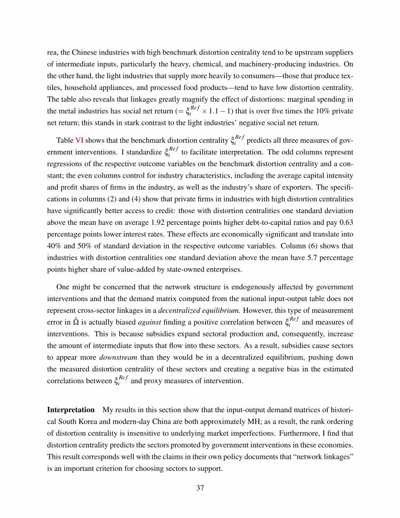
rea, the Chinese industries with high benchmark distortion centrality tend to be upstream suppliersof intermediate inputs, particularly the heavy, chemical, and machinery-producing industries. Onthe other hand, the light industries that supply more heavily to consumers—those that produce tex-tiles, household appliances, and processed food products—tend to have low distortion centrality.The table also reveals that linkages greatly magnify the effect of distortions: marginal spending inthe metal industries has social net return (= ξ
Re fi ×1.1−1) that is over five times the 10% private
net return; this stands in stark contrast to the light industries’ negative social net return.
Table VI shows that the benchmark distortion centrality ξRe fi predicts all three measures of gov-
ernment interventions. I standardize ξRe fi to facilitate interpretation. The odd columns represent
regressions of the respective outcome variables on the benchmark distortion centrality and a con-stant; the even columns control for industry characteristics, including the average capital intensityand profit shares of firms in the industry, as well as the industry’s share of exporters. The specifi-cations in columns (2) and (4) show that private firms in industries with high distortion centralitieshave significantly better access to credit: those with distortion centralities one standard deviationabove the mean have on average 1.92 percentage points higher debt-to-capital ratios and pay 0.63percentage points lower interest rates. These effects are economically significant and translate into40% and 50% of standard deviation in the respective outcome variables. Column (6) shows thatindustries with distortion centralities one standard deviation above the mean have 5.7 percentagepoints higher share of value-added by state-owned enterprises.
One might be concerned that the network structure is endogenously affected by governmentinterventions and that the demand matrix computed from the national input-output table does notrepresent cross-sector linkages in a decentralized equilibrium. However, this type of measurementerror in Ω is actually biased against finding a positive correlation between ξ
Re fi and measures of
interventions. This is because subsidies expand sectoral production and, consequently, increasethe amount of intermediate inputs that flow into these sectors. As a result, subsidies cause sectorsto appear more downstream than they would be in a decentralized equilibrium, pushing downthe measured distortion centrality of these sectors and creating a negative bias in the estimatedcorrelations between ξ
Re fi and proxy measures of intervention.
Interpretation My results in this section show that the input-output demand matrices of histori-cal South Korea and modern-day China are both approximately MH; as a result, the rank orderingof distortion centrality is insensitive to underlying market imperfections. Furthermore, I find thatdistortion centrality predicts the sectors promoted by government interventions in these economies.This result corresponds well with the claims in their own policy documents that “network linkages”is an important criterion for choosing sectors to support.
37

To be clear, my findings by no means suggest that polices adopted by these economies wereoptimal: my theory abstracts away from practical aspects of policy implementation, and there isalso substantial qualitative evidence that various political economy factors affected policy choicesin these economies (Krueger 1990; Robinson 2010). Nevertheless, my results indicate that thereare aspects of Korean and Chinese industrial strategy that appear to be motivated by a desire tosubsidize upstream sectors, and my theory shows that these interventions could create positivenetwork effects and improve aggregate productive efficiency.
7 Conclusion
Although industrial policies have been widely adopted by developing countries, economists’formal understanding of these policies remains limited. In this paper, I revisit Hirschman’s thesison the importance of cross-sector linkages for economic development, and I formally characterizeindustrial policies in production networks. I find that sectoral market imperfections accumulatethrough backward demand linkages and generate aggregate sales distortions that are largest in themost upstream sectors. This aggregate sectoral distortion, which I term distortion centrality, is asufficient statistic for the ratio between social and private marginal product of sectoral inputs; asa result, there is an incentive for a well-meaning government to subsidize the upstream sectors.My theoretical analysis therefore provides a counterpoint to the prevailing view that sector-basedselective interventions must be a sign of inefficiency.
Furthermore, I find that the ranking of sectoral distortion centrality is insensitive to marketimperfections if the production network exhibits monotone hierarchy property, and that the input-output structures of South Korea in the 1970s and modern-day China do approximately satisfy thisproperty. I show that distortion centrality predicts the sectors targeted by government interventionsin both of these economies, suggesting that certain aspects of their industrial strategy might havecreated positive network effects.
PRINCETON UNIVERSITY
38

References
Acemoglu, Daron, Ufuk Akcigit, and William Kerr (2016). Networks and the Macroeconomy: AnEmpirical Exploration. NBER Macroeconomics Annual.
Acemoglu, Daron, Vasco Carvalho, Asuman Ozdaglar, and Alireza Tahbaz-Salehi (2012). TheNetwork Origins of Aggregate Fluctuations. Econometrica.
Aghion, Philippe, Jing Cai, Mathias Dewatripont, Luosha Du, Ann Harrison, and Patrick Legros(2015). Industrial Policy and Competition. American Economic Journal: Macroeconomics.
Altinoglu, Levent (2017). The Origins of Aggregate Fluctuations in a Credit Network Economy.Working Paper.
Amsden, Alice (1989). Asia’s Next Giant: South Korea and Late Industrialization. Oxford Uni-versity Press.
Arrow, Kenneth and Frank Hahn (1971). General Competitive Analysis. North Holland.
Athey, Susan (2002). Monotone Comparative Statics Under Uncertainty. Quarterly Journal of
Economic Review.
Banerjee, Abhijit and Esther Duflo (2005). Growth Theory Through the Lens of DevelopmentEconomics. Handbook of Economic Growth.
Banerjee, Abhijit and Benjamin Moll (2010). Why does misallocation persist? American Eco-
nomic Journal: Macroeconomics.
Baqaee, David (2015). Labor Intensity in an Interconnected Economy. Working Paper.
Baqaee, David (2016). Cascading Failures in Production Networks. Working Paper.
Bartelme, Dominick and Yuriy Gorodnichenko (2015). Linkages and Economic Development.NBER Working Paper.
Bigio, Saki and Jennifer La’O (2016). Financial Frictions in Production Networks. NBER Working
Paper.
Boehm, Johannes (2017). The Impact of Contract Enforcement Costs on Outsourcing and Aggre-gate Productivity. Working Paper.
Boyreau-Debray, Genevieve and Shang-Jin Wei (2005). Pitfalls of a State-Dominated FinancialSystem: The Case of China. NBER Working Paper.
39

Buera, Francisco J. and Joseph P. Kaboski (2012). The Rise of the Service Economy. American
Economic Review.
Buera, Francisco J., Joseph P. Kaboski, and Yongseok Shin (2011). Finance and Development: ATale of Two Sectors. American Economic Review.
Buera, Francisco J., Joseph P. Kaboski, and Yongseok Shin (2015). Entrepreneurship and FinancialFrictions: A Macrodevelopment Perspective. Annual Review of Economics.
Caliendo, Lorenzo, Fernando Parro, and Aleh Tsyvinski (2017). Distortions and the Structure ofthe World Economy. Working Paper.
Calligaris, Sara, Massimo Del Gatto, Fadi Hassan, Gianmarco I.P. Ottaviano, and FabianoSchivardi (2016). Italy’s Productivity Conundrum: A Study on Resource Misallocation in Italy.European Economy Discussion Papers.
Chenery, Hollis, Sherman Robinson, and Moshe Syrquin (1986). Industrialization and Growth: A
Comparative Study, Edited by Hollis Chenery, Sherman Robinson and Moshe Syrquin. OxfordUniversity Press.
Cheremukhin, Anton, Mikhail Golosov, Sergei Gurieve, and Aleh Tsyvinski (2017a). The Econ-omy of People’s Republic of China from 1953. Working Paper.
Cheremukhin, Anton, Mikhail Golosov, Sergei Gurieve, and Aleh Tsyvinski (2017b). The indus-trialization and Economic Development of Russia through the Lens of a Neoclassical GrowthModel. Review of Economic Studies.
Chung, Young-Iob (2007). South Korea in the Fast Lane: Economic Development and Capital
Formation. Oxford University Press.
De Loecker, Jan and Frederic Warzynski (2012). Markups and Firm-Level Export Status. American
Economic Review.
Debla-Norris, Era, Si Guo, Vikram Haksar, Minsuk Kim, Kalpana Kochhar, Kevin Wiseman, andAleksandra Zdzienicka (2015). The New Normal: A Sector-Level Perspective on ProductivityTrends in Advanced Economies. IMF Staff Discussion Note.
Dollar, David and Shang-Jin Wei (2007). Das (Wasted) Kapital: Firm Ownership and InvestmentEfficiency in China. IMF Working Paper.
Fisman, Ray (2001). Trade Credit and Productive Efficiency in Developing Countries. World
Development.
40

Gale, David and Hukakane Nikaido (1965). The Jacobian Matrix and Global Univalence of Map-pings. Mathematische Annalen.
Gebresilasse, Mesay M. (2016). Industrial Policy and Misallocation in the Ethiopian Manufactur-ing Sector. Working Paper.
Hernandez, Zenaida (2004). Industrial Policy in East Asia: in Search for Lessons. World Devel-
opment Report Background Papers.
Hirschman, Albert O. (1958). The Strategy of Economic Development. Yale University Press.
Hsieh, Chang-Tai and Peter Klenow (2009). Misallocation and Manufacturing TFP in China andIndia. Quarterly Journal of Economics.
Hsieh, Chang-Tai and Zheng Michael Song (2015). Grasp the Large, Let Go of the Small. Brook-
ings Papers in Economic Activity.
Hulten, Charles (1978). Growth Accounting with Intermediate Inputs. Review of Economic Stud-
ies.
Jones, Chad (2013). Misallocation, Economic Growth, and Input-Output Economics. Advances in
Economics and Econometrics.
Kim, Eun Mee (1997). Big Business, Strong State: Collusion and Conflict in South Korean Devel-
opment, 1960-1990. Albany, NY: State University of New York Press.
Krueger, Anne O. (1990). Government Failures in Development. Journal of Economic Perspec-
tives.
Kuo, Shirley W.Y. (1983). The Taiwan Economy in Transition. Boulder, Colorado: Westview.
Leal, Julio (2015). Key Sectors in Economic Development: A Perspective from Input-OutputLinkages and Cross-Sector Misallocation. Working Paper.
Leal, Julio (2017). Cross-Sector Misallocation with Sector-Specific Distortions. The World Bank
Economic Review.
Leontief, Wassily (1963). The Structure of Development. Scientific American.
Li, Kwoh-ting and Tzong-Shian Yu (1982). Experiences and Lessons of Economic Development
in Taiwan. Taipei: Academic Sinica.
41

Midrigan, Virgiliu and Daniel Yi Xu (2014). Finance and Misallocation: Evidence from Plant-Level Data. American Economic Review.
Murphy, Kevin M., Andrei Shleifer, and Robert W. Vishny (1989). Industrialization and the BigPush. Journal of Political Economy.
Nabli, Mustapha K., Jennifer Keller, Claudia Nassif, and Carlos Silva-Jauregui (2006). The Po-litical Economy of Industrial Policy in the Middle East and North Africa. World Bank Working
Paper.
Page, John (1994). The East Asian Miracle: Four Lessons for Development Policy. NBER Macroe-
conomics Annual.
Restuccia, Diego and Richard Rogerson (2008). Policy distortions and aggregate productivity withheterogeneous establishment. Review of Economic Dynamics.
Riedel, James, Jing Jin, and Jian Gao (2007). How China grows: investment, Finance, and Reform.Princeton and Oxford: Princeton University Press.
Robinson, James (2010). Industrial Policy and Development: A Political Economy Perspective.Annual World Bank Conference on Development Economics Global.
Rodrik, Dani (2004). Industrial Policy for the Twenty-First Century. Working Paper.
Rodrik, Dani (2008). Normalizing Industrial Policy. Commission on Growth and Development
Working Paper No. 3.
Rosenstein-Rodan, Paul (1943). Problems of Industrialization of Eastern and South-Eastern Eu-rope. The Economic Journal.
Rotemberg, Martin (2017). Equilibrium Effects of Firm Subsidies. Working Paper.
Ruiz, Elena Martinez (2003). Autarkic Policy and Efficiency in the Spanish Industrial Sector. AnEstimate of Domestic Resource Cost in 1958. Working Paper.
Song, Zheng Michael, Kjetil Storesletten, and Fabrizio Zilibotti (2011). Growing Like China.American Economic Review.
State Development Planning Commission of China (1995). Strategy for Chinese Pillar Industries
(in Chinese: Zhong Guo Zhi Zhu Chan Ye Zhen Xing Fang Lue).
Stiglitz, Joseph (1970). Non-Substitution Theorems with Durable Capital Goods. Review of Eco-
nomic Studies.
42

Sun, Pei (2009). Rent Allocation and Industrial Policy Efficacy in the Steel Industry. Rent Seeking
in China: edited by Tak-Wing Ngo, Yongping Wu.
Wade, Robert (1989). What Can Economics Learn from East Asian Success? The Annals of the
American Academy of Political and Social Science.
Westphal, Larry E. (1990). Industrial Policy in an Export-Propelled Economy: Lessons from SouthKorea’s Experience. Journal of Economic Perspective.
Woo, Jung-en (1991). Race to the Swift: State and Finance in Korean Industrialization. New York:Columbia University Press.
Woo-Cumings, Meredith (2001). Miracle as Prologue : the State and the Reform of the CorporateSector in Korea. Rethinking the East Asian Miracle.
Yang, Ya-Hwei (1993). Government Policy and Strategic Industries: The Case of Taiwan. Trade
and Protectionism, NBER-EASE Volume 2.
43

Table I: Exhaustively testing the MH inequalities in Definition (8) shows that the input-outputdemand matrices of both South Korea and China are approximately MH
Fraction of inequalities Sum of truncated entriesTruncation that hold true over sum of all entries in Ω
threshold South Korea China South Korea China
no truncation 86% 72% 0 00.0001 91% 79% 0.001 0.0010.0005 96% 86% 0.007 0.0080.001 97% 92% 0.016 0.020
This table shows that the input-output demand matrices for South Korea and China are approxi-mately MH. The first two columns report, for each country, the fraction of inequalities in Defini-tion (8) that hold true, over all unique combinations of industries. The first row shows the resultsperformed directly on the input-output demand matrices. The remaining rows conduct the sameexercise but replace ωi j < w to zero, where w is the truncation threshold and takes the value of0.0001, 0.0005, and 0.001, respectively for rows 2-4. These small entries represent weak input-output demand relationships and are unimportant in determining sectoral distortion centrality, c.f.Theorem 4. As the last two columns show, the sum of truncated entries is minuscule relative to thesum of all entries in the input-output demand matrices for both countries.
44
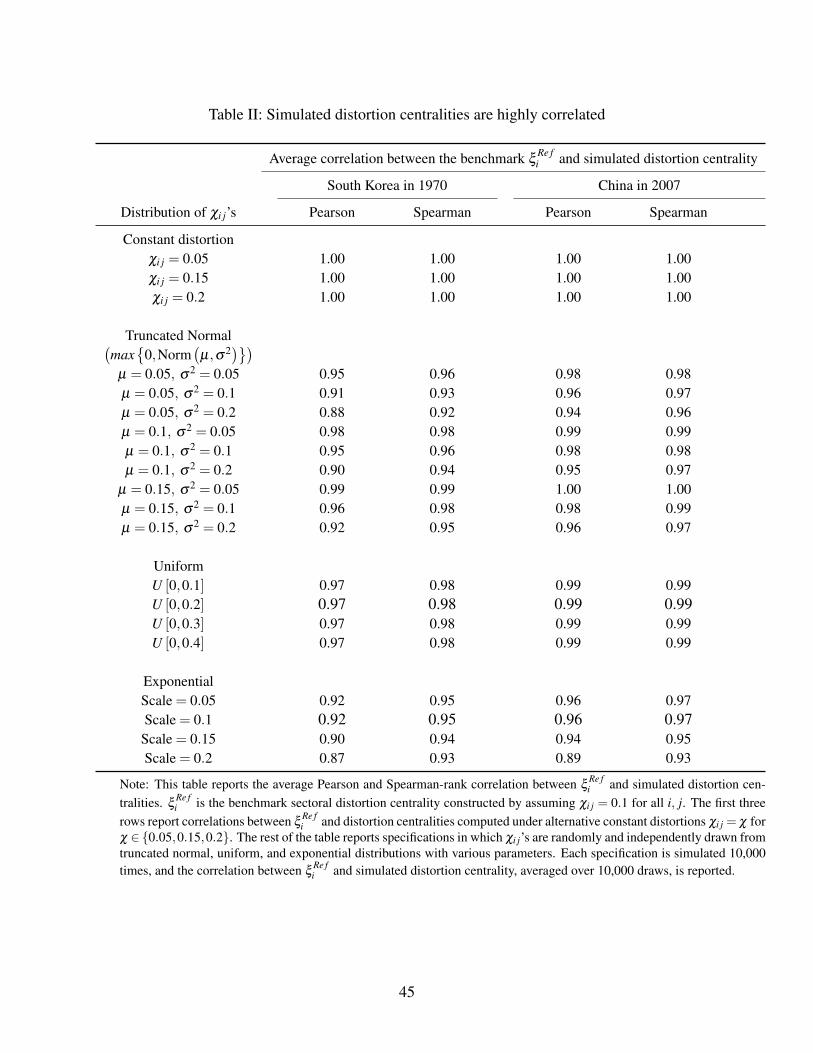
Table II: Simulated distortion centralities are highly correlated
Average correlation between the benchmark ξRe fi and simulated distortion centrality
South Korea in 1970 China in 2007
Distribution of χi j’s Pearson Spearman Pearson Spearman
Constant distortionχi j = 0.05 1.00 1.00 1.00 1.00χi j = 0.15 1.00 1.00 1.00 1.00χi j = 0.2 1.00 1.00 1.00 1.00
Truncated Normal(max
0,Norm
(µ,σ2
))µ = 0.05, σ2 = 0.05 0.95 0.96 0.98 0.98µ = 0.05, σ2 = 0.1 0.91 0.93 0.96 0.97µ = 0.05, σ2 = 0.2 0.88 0.92 0.94 0.96µ = 0.1, σ2 = 0.05 0.98 0.98 0.99 0.99µ = 0.1, σ2 = 0.1 0.95 0.96 0.98 0.98µ = 0.1, σ2 = 0.2 0.90 0.94 0.95 0.97
µ = 0.15, σ2 = 0.05 0.99 0.99 1.00 1.00µ = 0.15, σ2 = 0.1 0.96 0.98 0.98 0.99µ = 0.15, σ2 = 0.2 0.92 0.95 0.96 0.97
UniformU [0,0.1] 0.97 0.98 0.99 0.99U [0,0.2] 0.97 0.98 0.99 0.99U [0,0.3] 0.97 0.98 0.99 0.99U [0,0.4] 0.97 0.98 0.99 0.99
ExponentialScale = 0.05 0.92 0.95 0.96 0.97Scale = 0.1 0.92 0.95 0.96 0.97
Scale = 0.15 0.90 0.94 0.94 0.95Scale = 0.2 0.87 0.93 0.89 0.93
Note: This table reports the average Pearson and Spearman-rank correlation between ξRe fi and simulated distortion cen-
tralities. ξRe fi is the benchmark sectoral distortion centrality constructed by assuming χi j = 0.1 for all i, j. The first three
rows report correlations between ξRe fi and distortion centralities computed under alternative constant distortions χi j = χ for
χ ∈ 0.05,0.15,0.2. The rest of the table reports specifications in which χi j’s are randomly and independently drawn fromtruncated normal, uniform, and exponential distributions with various parameters. Each specification is simulated 10,000times, and the correlation between ξ
Re fi and simulated distortion centrality, averaged over 10,000 draws, is reported.
45

Table III: Targeted HCI industries have higher distortion centrality than non-targeted industries inSouth Korea in 1970
Average E [ξi] Share of industries with E [ξi]> 1
Distribution of χi j HCI non-HCI HCI non-HCI
χi j = 0.1 1.21 1.03 100% 56.7%Truncated Normal 1.21 1.03 100% 55.0%
Uniform 1.21 1.03 100% 55.0%Exponential 1.21 1.03 100% 56.7%
This table shows that the targeted HCI industries have higher distortion centralities on average thanthe non-targeted industries, and a higher fraction of targeted industries have distortion centralitiesabove unity. The first row is based on ξ
Re fi , the benchmark distortion centrality under the assump-
tion that χi j = 0.1 in all sectors and for all inputs. The remaining rows report results using sim-ulated distortion centrality, respectively computed by drawing χi j’s i.i.d. from truncated normal(max0,Norm(0.09,0.1)), uniform (U [0,0.2]), and exponential (with scale 0.1) distributions.For each specification, E [ξi] is computed as the average distortion centrality of industry i over10,000 simulations. The parameters used for simulating χi j’s are chosen such that E
[χi j]= 0.1
under all three distributions; this makes the simulated distortion centrality comparable in levelsto ξ
Re fi . Additional specifications in Appendix Table B.1 show that results are quantitatively and
qualitatively robust to alternative parametrizations: 1) all HCI industries have E [ξi] > 1; 2) ex-pected social net return to spending in the HCI sector is over three times of the private net return
(E[ξi]×E[PRi j]−1
E[PRi j]−1); 3) around 45% of non-targeted industries have expected distortion centrality be-
low one.
46

Table IV: Distortions on the purchase of non-targeted goods have to be enormous in order fortargeted and non-targeted industries to have the same average distortion centralities
χ 0.01 0.02 0.03 0.04 0.05 0.06 0.07 0.08 0.09 0.1α 520% 525% 530% 533% 534% 538% 540% 544% 547% 550%
This table shows that in order for the non-targeted industries to have higher distortion centralityon average than the HCI industries, the distortions on the purchases of non-targetedmanufacturing goods have to be enormous relative to distortions on goods produced by thetargeted industries. Specifically, for each (χ,α), I let χi j = χ for all j’s produced by the HCIindustries and χi j = α ·χ for all j’s produced by the non-targeted industries. I compute distortioncentrality ξi (χ,α) as functions of χ and α . The table reports, for a range of χ’s, the smallest α
under which the targeted and non-targeted manufacturing industries have the same averagedistortion centralities.
47

Table V: The top and bottom ten Chinese manufacturing industries by distortion centrality in 2007
Top 10 ξRe fi Bottom 10 ξ
Re fi
Coke making 1.43 Misc. food products 0.77Ferrous alloy 1.42 Meat processing 0.84Iron smelting 1.41 Medicinal chemicals 0.84Nonferrous metal smelting 1.40 Grain mill products 0.87Metal cutting machinery 1.39 Textile, clothing and footwear 0.88Steel smelting 1.39 Seafood processing 0.88Railroad equipment 1.36 Household AV Equipment 0.89Industrial furnace and boiler 1.35 Liquor and alcoholic drinks 0.90Manufacturing of basic chemicals 1.33 Household Appliances 0.91Refining and rolling of nonferrous metals 1.32 Vegetable oil products 0.91
48

Table VI: Chinese manufacturing industries with high distortion centrality receive more govern-ment support: 1) privately-owned firms in these industries have better access to credit markets, and2) these industries have more state-owned enterprises
SOE Share ofDebt-To-Capital Ratio Interest Rate Value-Added
(1) (2) (3) (4) (5) (6)
ξRe fi (standardized) 1.842∗∗∗ 1.919∗∗∗ −0.382∗∗ −0.627∗∗∗ 9.537∗∗∗ 5.735∗∗∗
(0.533) (0.483) (0.142) (0.117) (2.167) (1.963)
Capital Intensity 0.563 −1.810∗∗∗ 2.305(1.631) (0.394) (6.636)
Profit Share −2.716∗∗∗ 0.443∗∗∗ −0.778(0.499) (0.121) (2.032)
Share of Exporters −4.999 −3.209∗∗∗ −64.74∗∗∗
(3.062) (0.740) (12.46)
Outcome Mean & 54.78 2.68 21.76Standard Deviation [4.88] [1.26] [20.79]
Controls No Yes No Yes No YesAdjusted R2 0.144 0.399 0.088 0.472 0.220 0.452
# Obs. 66 66 66 66 66 66
The table examines the correlation between standardized benchmark distortion centrality ξRe fi and measures of gov-
ernment interventions extracted from the 2007 edition of China’s Annual Industrial Survey. Columns (1) and (2) showthat ξ
Re fi predicts the average debt-to-capital ratio for privately-owned firms in the industry; columns (3) and (4) show
that ξRe fi predicts the average effective interest rate for privately-owned firms in the industry; columns (5) and (6)
show that ξRe fi predicts the share of industry value-added that is contributed by state-owned enterprises. Columns (1),
(3), and (5) regress the respective outcome variables on ξRe fi and a constant, while columns (2), (4), and (6) control
for the average capital intensity and the average profit share of revenue for firms in the industry, as well as the shareof exporters in the industry. Standard errors are shown in parenthesis. Industry averages of firm-level variables arecomputed after dropping outliers at 1%. Debt-to-capital is computed as the 100×the ratio between total outstandingdebt at the end of the year and the total reported capital. Effective interest rate is computed as 100×total interestpayment in 2007 divided by the total outstanding debt at the end of the year. Capital intensity is computed as the ratiobetween reported capital and firm revenue. Profit share is computed as 100×profits divided by revenue. A firm isidentified as an exporter if it reported a positive amount of exports. SOEs are identified using the procedure outlinedin Hsieh and Song (2015).
49

Figure I: Illustration of the vertical production economy
50

Figure II: An illustrative input-output matrix of a monotone-hierarchical network
Inpu
t-Usi
ng In
dust
ries
Input-Supplying Industries
The figure visualizes a hypothetical lower-triangular Ω matrix that satisfies the MH property. Rowsrepresent input-using industries and columns represent input-supplying industries. The i j-th entryin the figure corresponds to ωi j, the faction of (column) good j that is supplied to (row) industry i.The size of each entry is drawn proportionally to ωi j.
51

Figure III: Input-output demand matrix of South Korea in 1970
Inpu
t-Usi
ng In
dust
ries
Input-Supplying Industries
The input-using industry was targeted by HCI driveAll others
The figure visualizes the input-output demand matrix Ω of South Korea in 1970. Rows representinput-using industries and columns represent input-supplying industries. The i j-th entry in thefigure corresponds to ωi j, the faction of (column) good j that is supplied to (row) industry i. Cellsfor which the input-using industry was promoted by the HCI drive are highlighted with solid blackcircles. The size of each entry is drawn proportionally to ωi j and is truncated below at 5%, so thatonly important input-output demand relationships are represented in the figure. A line is drawnacross the diagonal entries.
The figure reveals that the relationship of input-flows is highly asymmetric across the targeted andnon-targeted groups of industries. The targeted ones are upstream: they supply to the non-targeteddownstream industries while purchasing few intermediate inputs in return, resulting in an approx-imately lower-triangular input-output demand matrix. This pattern only emerges after industriesare ordered by their distortion centrality—in this case, industries are arranged in decreasing orderof ξ
Re fi , the sectoral distortion centrality under the assumption that distortions are uniform across
all sectors and all inputs with χi j = 0.1.52

Figure IV: Input-output demand matrix of China in 2007In
put-U
sing
Indu
strie
s
Input-Supplying Industries
The figure visualizes the input-output demand matrix Ω of China in 2007. Rows represent input-using industries and columns represent input-supplying industries. The i j-th entry in the figurecorresponds to ωi j, the faction of (column) good j that is supplied to (row) industry i. The sizeof each entry is drawn proportionally to ωi j and is truncated below at 5%, so that only importantinput-output demand relationships are represented in the figure. A line is drawn across the diagonalentries. Industries are arranged in decreasing order of ξ
Re fi , the sectoral distortion centrality under
the assumption that distortions are uniform across all sectors and all inputs with χi j = 0.1.
53

Appendix
A Proofs
A.1 Proof of Lemma 1
The market clearing condition for good j is
Q j = Yj +∑i∈S
Mi j.
Multiplying both sides by Pj/WL and using the fact that γ j ≡PjQ jWL and β j ≡
PjY jY , we obtain
γ j =Y
WLβ j +∑
i∈Sωi jγi
or in matrix notation,γ′ =
YWL·β ′ (I−Ω)−1 .
The labor share in the economy sums to one, which implies that ∑i∈S ωLi γi = 1. Therefore it must
be the case that WLY = β ′ (I−Ω)−1
ωL, as desired.
A.2 Proof of Proposition 1
The equilibrium prices Pi and W form the fixed point to the system of equations
Pi = Ci(W,
Pj
;zi)
for i ∈ S;
1 = C F (Pj)
.
Totally differentiating, we obtain
d lnPi =−d lnzi +σLi d lnW + ∑
j∈Sσi jd lnPj
0 = ∑j∈S
β jd lnPj
54

or in matrix form,
d lnP = −d lnz+σLd lnW +Σd lnP
= (I−Σ)−1 (−d lnz+σLd lnW
)0 = β
′d lnP.
Combining the two equations, we get that
d lnPd lnzi
= (I−Σ)−1(
σL · d lnW
d lnzi− ei
)and
d lnWd lnzi
=β ′ (I−Σ)−1 · ei
β ′ (I−Σ)−1σL
= µi
where the last equality follows because β ′ (I−Σ)−1σL = 1 under the assumption that all produc-
tion functions have constant-returns-to-scale.
A.3 Proof of Lemma 3
Following the proof for Proposition 1, we can write the equilibrium prices Pi and W as thefixed point to the system of equations
Pi = Ci(W,
Pj
;
χi j)
for i, j ∈ S;
1 = C F (Pj)
. (A.1)
Differentiating the first equation with respect to 1+χi j and stacking into a vector, we get
d lnPd ln(1+χi j
) = (I−Σ)−1
(−σi j · ei +σ
L d lnWd ln(1+χi j
)) , (A.2)
which proves part 1 of the lemma. Differentiating (A.1) gets us
0 = β′ d lnPd ln(1+χi j
) . (A.3)
55

Plugging equation (A.2) into (A.3), we get
d lnWd ln(1+χi j
) =−µi ·σi j.
In absence of public consumption, C =WL and we have d lnCd ln(1+χi j)
=−µi ·σi j as desired.
A.4 Proof of Theorem 1
First, note that the marginal cost of implementing subsidy τik is
d(
τik1+τik
PkMik
)dτik
∣∣∣∣∣τik=0
= PkMik.
That is, for ∆ units (a small amount) of additional resources available to the economy, the level ofsubsidy that can be implemented is τik =
∆
PkMik.
The marginal gain in aggregate consumption that results from the subsidy τik, starting from thedecentralized equilibrium, is captured by
d lnCd ln(1+ τik)
∣∣∣∣∣τik=0
= µi ·σik.
The expression is a direct corollary of Lemma 3, because the effect of d ln(1+ τik) on aggregateconsumption is similar to that of a marginal decrease in distortion χik. The expression is alsointuitive in light of Lemma 2 and Proposition 1: σik captures the partial equilibrium effect of τik
on the sectoral unit cost of production while holding all input prices constant, and µi captures thegeneral equilibrium effect on aggregate consumption resulting from a proportional shift in Ci (·),the mapping from input prices to the unit cost of production. The total effect of τik on aggregateconsumption C is the product of the partial and general equilibrium effects.
The social marginal return is obtained by dividing the marginal change in consumption and therequired expenditure,
SRik =dC/dτik
d(
PkMik · τik1+τik
)/dτik
∣∣∣τik=0
.
The numerator can be written as dC/dτik = C ·d lnC/d ln(1+ τik) whereas the denominator sim-
56

plifies tod(
PkMik · τik1+τik
)dτik
∣∣∣∣∣τik=0
=
(PkMik +
d (PkMik)
dτik· τik
1+ τik
)∣∣∣∣∣τik=0
= PkMik.
Therefore we have
SRik =C
PkMik· d lnC
d ln(1+ τik)
=µi ·σik
PkMikPiQi· PiQi
C
= PRik ·ξi,
as desired.
A.5 Proof of Theorem 2
In the presence of public consumption E, it is no longer the case that C =WL. Nevertheless, adirect corollary from Lemma 3 is that d lnWL
d ln(1+τik)= µi ·σik. Now consider a marginal change in τik
financed by cutting back E while holding the lump-sum tax T constant. From the budget constraintof the representative consumer (WL =C+T ), we derive
dWLd ln(1+ τik)
=dC
d ln(1+ τik)=WL ·µi ·σik.
From the planner’s fiscal constraint (E + τik1+τik
PkMik = T ), we derive
dEd ln(1+ τik)
=−d(
τik1+τik
PkMik
)d ln(1+ τik)
.
57

Therefore the social return of expenditure on τik is
SRik ≡ −dC/dτik
dE/dτik
∣∣∣∣∣τik=0,T constant
=WL ·µi ·σik.
d(
τik1+τik
PkMik
)d ln(1+τik)
∣∣∣∣∣τik=0,T constant
=µi ·σik.
PkMikPiQi· PiQi
WL
= PRik ·ξi,
as desired.
A.6 Proof of Proposition 2
The transfer ηi induces sectoral allocations that are equivalent to a subsidy on the purchase ofthe constrained inputs, with (
1+ τKi)≡ Γi +ηi
Γi.
Also note that the Lagrange multiplier χi is equal to
1+χi =∑ j∈Di σi j
∑ j∈Di ωi j,
and therefore it captures the private return to a subsidy τKi that applies to inputs in the constrained
set Di.
The social return on the grant of working capital is
SRKi ≡ dC/dηi
dE/dηi
∣∣∣∣∣ηi=0,T constant
=dC/dτK
idE/dτK
i
∣∣∣∣∣ηi=0,T constant
= (1+χi)×ξi
where the last equality follows from Corollary 1.
58

A.7 Proof of Proposition 3
Note that sales subsidy can be interpreted as a subsidy, applied to all sectoral inputs, that shiftsthe sectoral cost function in a Hicks-neutral way. Sectoral constant-returns-to-scale implies
S
∑j=1
(1+χi j
)ωi j =
S
∑j=1
σi j = 1 for all i.
The result is therefore a direct application of Corollary 1, recognizing that the private return tosales subsidy is equal to one.
A.8 Proof of Theorem 3
To prove Theorem 3, consider a Cobb-Douglas economy with subsidies(1+ τL). The sectoral
allocations satisfyPjMi j = ωi jPiQi, WLi =
(1+ τ
Li)
ωLi PiQi
where
ωi j =σi j
1+χi j, ω
Li =
σLi
1+χLi.
Note that under Cobb-Douglas assumptions,
σi j,ωi jS
i, j=1,
σLi ,ω
LiS
i=1, and consequently µi,γiSi
are all stable and do not change in response to value-added subsidies.
We can solve for the quantity of inputs as
Mi j = ωi jγi
γ jQ j, Li =
(1+ τ
Li)
ωLi γiL.
Labor market clearing yields
∑i
(1+ τ
Li)
ωLi γi = 1.
Sectoral output can be written as
lnQi = lnzi +σLi lnLi +∑
jσi j lnMi j
= ζi +σLi(ln(1+ τ
Li)+ lnγi
)+∑
jσi j(lnγi + lnQ j− lnγ j
)
59

whereζi ≡ lnzi +σ
Li lnω
Li +σ
Li lnL+∑
jσi j lnωi j.
Constant-returns-to-scale implies σLi +∑ j σi j = 1 hence
lnQi− lnγi = ζi +σLi ln(1+ τ
Li)+∑
jσi j(lnQ j− lnγ j
).
Since γi ≡ PiQiWL , we have lnQi− lnγi = lnWL− lnPi and we can stack the equation above into a
vector equation aslnWL− lnP = (I−Σ)−1 (
ζ +σL ln
(1+ τ
L))By normalizing the price of the final good to be one, we know
β′ (lnP− lnβ ) = 1
where ∑Si=1 βi = 1. Thus
lnWL = constant+β′ (I−Σ)−1 (
σL ln
(1+ τ
L)) .Now to find the constrained-optimal value-added subsidies, we solve
maxτL
i lnW
(τ
Li)
s.t.S
∑i=1
τLi WLi = T.
Let λ be the Lagrange multiplier on the planner’s budget constraint. The first-order condition withrespect to τL
i is
d lnWd ln(1+ τL
i) · 1
1+ τLi
= λ
[WLi +
(S
∑i=1
τLi WLi
)d lnW
d ln(1+ τL
i) · 1
1+ τLi
]
=λ
1−λTWLi
or equivalentlyµiσ
Li
1+ τLi
∝(ω
Li γi).
We therefore have (1+ τ
Li)
∝ ξi(1+χ
Li),
as desired. Note that the result is stated in terms of proportionality because the level of taxes
60

depends on the lump-sum tax T to which the planner has access.
A.9 Proof of Theorem 4
Let δ ≡ WLY . Sectoral influence is
µ j = β j +∑i∈S
µiσi j
Dividing influence by sales, we get
ξ j =β j
γ j+∑
i∈S
µiσi j
γ j
=Yj/Y
PjQ j/WL+∑
i∈S
µi
γi
γi
γ j
σi j
ωi jωi j
= ωFj ·δ +∑
i∈Sξi(1+χi j
)ωi j,
or in matrix form,ξ′ = δ ·
(ω
F)′ (I−D Ω)−1
,
where D≡[1+χi j
]is the matrix of underlying sectoral distortions.
A.10 Proof of Proposition 4
Lemma 4. Let X ≡x,x+1, · · · , x and Y be ordered sets. Suppose ami ∈R≥0 is log-supermodular
in (m, i) ∈ X×Y and ∑m∈X ami = ∑m∈X am j < ∞ for all i, j ∈ Y . Then we have
1. ∑Km=x ami ≥ ∑
Km=x am j for all K ∈ X and i < j ∈ Y ;
2. If bmm∈X is a non-increasing and non-negative sequence, then
∑m∈X
amibm ≥ ∑m∈X
am jbm for i < j ∈ Y.
Proof. Consider i < j ∈ Y . Log-supermodularity implies that for m < n ∈ X ,
amian j ≥ am jani.
61

Now consider the sum ∑Km=x ami. Log-supermodularity again implies that for all n > K ∈ X ,(
K
∑m=x
ami
)an j ≥
(K
∑m=x
am j
)ani.
Summing over n = K +1, · · · , x, we have(K
∑m=x
ami
)(x
∑n=K+1
an j
)≥
(K
∑m=x
am j
)(x
∑n=K+1
ani
).
Let c≡ ∑m∈X ami ≥ 0. Then the inequality can be re-written as(K
∑m=x
ami
)(c−
(K
∑m=x
am j
))≥
(K
∑m=x
am j
)(c−
(K
∑m=x
ami
))
which implies (K
∑m=x
ami
)≥
(K
∑m=x
am j
),
proving the first part of the lemma. Note that this result also implies that(x
∑m=K
ami
)≤
(x
∑m=K
am j
)for all K ∈ X and i < j ∈ Y.
To show the second part, note that
x
∑m=x
amibm =x
∑m=x
amibx +x−1
∑m=x
ami (bm−bx)
=x
∑m=x
amibx +x−1
∑m=x
ami (bx−1−bx)+x−2
∑m=x
ami (bm−bx−1)
...
= bx
x
∑m=x
ami +x−x
∑k=1
((bx−k−bx−(k−1)
) x−k
∑m=x
ami
)
≥ bx
x
∑m=x
am j +x−x
∑k=1
((bx−k−bx−(k−1)
) x−k
∑m=x
am j
)
=x
∑m=x
am jbm,
where the inequality follows from part 1 of the lemma and the fact that(bx−k−bx−(k−1)
)≥ 0 since
62

bm is non-increasing.
Lemma 5. The product of two MH matrices is MH.
Proof. Let A and B be two S×S matrices that are MH. Let εA be the S×1 vector with entries εAi ≡
1−∑Sm=1 Ami, and define the vector εB ≡
[1−∑
Sm=1 Bmi
]Si=1 accordingly. Define (S+1)× (S+1)
matrices ΓA and ΓB as follows:
ΓA ≡
[A 0(
εA)′ 1
], Γ
B ≡
[B 0(
εB)′ 1
].
Both ΓA and ΓB are stochastic matrices with columns summing to one, and both are log-supermodularin their entries given that A and B are MH. Multiplying ΓA and ΓB, we get
(Γ
AΓ
B)
mi=
S
∑k=1
ΓAmkΓ
Bki,
and because log-supermodularity is preserved under multiplication and integration, we have that(ΓAΓB) is log-supermodular in its entries. Furthermore, it is also a stochastic matrix with column
sums equal to one. Lastly, note that the i j-th entry of (A×B) is precisely the i j-th entry of ΓAΓB
for all i, j ≤ S, thus establishing that (A×B) is MH.
Lemma 6. If A is an S×S MH matrix, its column sum is non-increasing:
S
∑m=1
Ami ≥S
∑m=1
Am j for i < j.
Proof. Define ΓA as in the proof of Lemma 5 and apply the first result of Lemma 4.
A.10.1 Proof of Case 1
First note thatµ′ = β
′ (I−Σ)−1 , γ’ ∝ β′ (I−Ω)−1
implies that there exist a constant c such that
cµ′ (I−Σ) = γ
′ (I−Ω)
orcµ′− γ
′ = cµ′Σ− γ
′Ω.
63

We write out the j-th entry of the equation above and divide both sides by γ j,
cµ j− γ j
γ j= ∑
i
cµiσi j− γiωi j
γi
γi
γ j
= ∑i
(cµi− γi)σi j + γi(σi j−ωi j
)γi
γi
γ j
= ∑i
(cµi− γi)ωi j(1+χi j
)+ γiωi jχi j
γi
γi
γ j
= ∑i
(cµi− γi
γiωi j(1+χi j
)+ ωi jχi j
).
In vector form,
cξ′−1′ =
(cξ′−1′
)(D Ω
)+1′D Ω−1′Ω
implying
cξ′−1′ = 1′
(D Ω− Ω
)(I−D Ω
)−1
=∞
∑k=0
1′(D Ω− Ω
)(D Ω
)k.
Since(D Ω− Ω
)and
(D Ω
)are both MH, we know that for all k,
(D Ω− Ω
)(D Ω
)kis MH
according to Lemma 5 and therefore has non-increasing column sums according to Lemma 6. Asa result, ξ must be non-increasing, as desired.
A.10.2 Proof of Case 2
Suppose Ω is MH and lower-triangular. Let di ≡ 1δ
ξi, and ωS+1,S ≡ ωFS to simplify notation.
From Theorem (4) and the fact that Ω is lower-triangular, we have
dS = ωS+1,S + ωS,S(1+χS,S
)dS
=ωS+1,S
1− ωS,S(1+χS,S
) .Because of sectoral constant-returns-to-scale and the fact that σL
i > 0 in any equilibrium underAssumption 1, the denominator has to be positive since ωS,S
(1+χS,S
)= ωS,S
(1+χS,S
)= σS,S <
1. We therefore have dS ≥ωS+1,S1−ωS,S
= 1 where the equality comes from the market clearing condition
64

of good S(ωS,S + ωS+1,S = 1
). Further,
dS−1 =ωS+1,S−1 + ωS,S−1dS
(1+χS,S−1
)1− ωS−1,S−1
(1+χS−1,S−1
)≥
ωS+1,S−1 + ωS,S−1dS(1+χS,S−1
)1− ωS−1,S−1
.
By MH, we haveωS,S−1ωS+1,S ≥ ωS,SωS+1,S−1.
We now use Lemma 4 to show E[dS−1
∣∣χkkSk=1
]≥E
[dS∣∣χkkS
k=1
]. Let as,S≡ ωs,S and as,S−1≡
ωs,S−11−ωS−1,S−1
for s ∈ S,S+1. By construction, as,s′ is log-supermodular in (s,s′) ∈ S,S+1×S−1,S and ∑s∈S,S+1 as,S−1 = ∑s∈S,S+1 as,S = 1. Furthermore, let
bS+1 = 1, bS = E[dS(1+χS,S−1
)∣∣χkkSk=1
];
thus bs is a non-increasing sequence for s ∈ S,S+1. Applying Lemma 4, we have
E[dS−1
∣∣χkkSk=1
]≥
ωS+1,S−1 + ωS,S−1E[dS(1+χS,S−1
)∣∣χkkSk=1
]1− ωS−1,S−1
≥ ωS+1,S + ωS,SE[dS(1+χS,S−1
)∣∣χkkSk=1
]≥ ωS+1,S + ωS,SE
[dS(1+χS,S
)∣∣χkkSk=1
]= E
[dS∣∣χkkS
k=1
]where the second inequality follows from the second part of the Lemma 4 and the third inequalityfollows from the assumption that χS,S ≤ χS,S−1 almost surely.
We now apply induction. Suppose E[ds∣∣χkkS
k=1
]≥ E
[ds+1
∣∣χkkSk=1
]for s = m+ 1,m+
2, · · · ,S. We have that for all s≥ m+1,
E[ds (1+χs,m+1)
∣∣χkkSk=1
]= E
[ds∣∣χkkS
k=1
]E[(1+χs,m+1)
∣∣χkkSk=1
]≥ E
[ds+1
∣∣χkkSk=1
]E[(1+χs+1,m+1)
∣∣χkkSk=1
]= E
[ds+1 (1+χs+1,m+1)
∣∣χkkSk=1
].
In other words, E[ds (1+χs,m+1)
∣∣χkkSk=1
]form a non-increasing sequence in s ≥ m+ 1. We
65

also have
dm+1 = ωS+1,m+1 +S
∑n=m+1
ωn,m+1dn (1+χn,m+1)
dm =ωS+1,m +∑
Sn=m+1 ωn,mdn (1+χn,m)
1− (1+χm,m) ωm,m
≥ωS+1,m +∑
Sn=m+1 ωn,mdn (1+χn,m)
1− ωm,m.
Now let as,m+1 = ωs,m+1 and as,m =ωs,m
1−ωm,mfor s∈m+1,m+2, · · · ,S+1. as,s′ is log-supermodular
and ∑S+1s=m+1 as,m = ∑
S+1s=m+1 as,m+1 = 1. We therefore have
E[dm+1
∣∣χkkSk=1
]= ωS+1,m+1 +
S
∑n=m+1
ωn,m+1E[dn (1+χn,m+1)
∣∣χkkSk=1
]
≤ωS+1,m +∑
Sn=m+1 ωn,mE
[dn (1+χn,m+1)
∣∣χkkSk=1
]1− ωm,m
≤ωS+1,m +∑
Sn=m+1 ωn,mE
[dn (1+χn,m)
∣∣χkkSk=1
]1− ωm,m
≤ E[dm∣∣χkkS
k=1
].
The second line follows from Lemma 4 and the fact that E[ds (1+χs,m+1)
∣∣χkkSk=1
]is non-
increasing in s; the third line follows by the conditional independence of χi j’s. By induction, wehave that E
[di∣∣χkkS
k=1
]≥ E
[d j∣∣χkkS
k=1
]for all i < j. Applying the law of iterated expecta-
tions, we have E [di]≥ E[d j]
for all i < j, as desired.
66
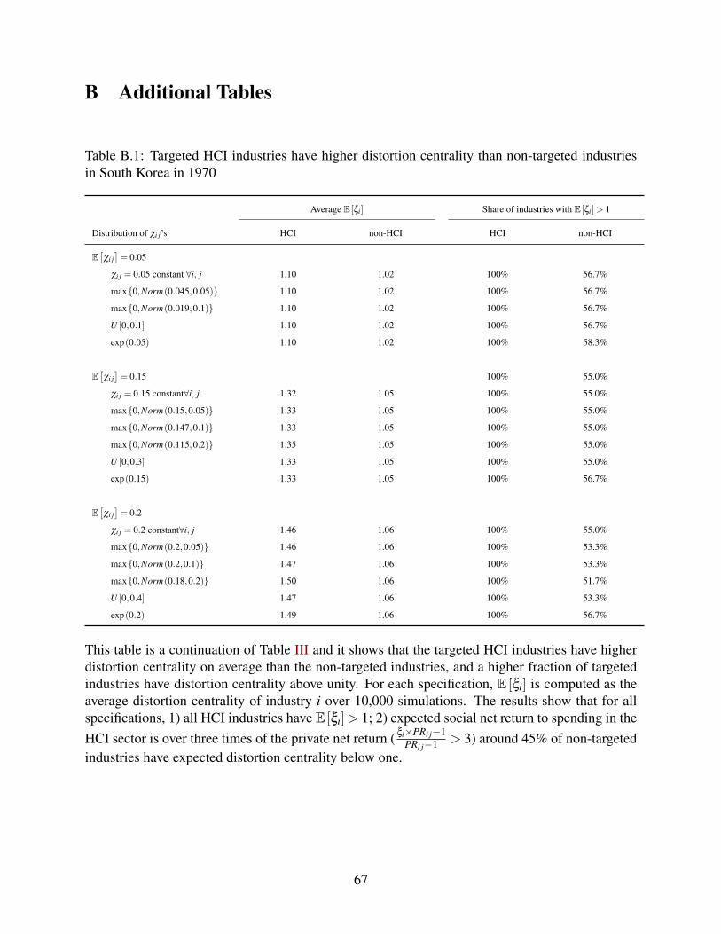
B Additional Tables
Table B.1: Targeted HCI industries have higher distortion centrality than non-targeted industriesin South Korea in 1970
Average E [ξi] Share of industries with E [ξi]> 1
Distribution of χi j’s HCI non-HCI HCI non-HCI
E[χi j]= 0.05
χi j = 0.05 constant ∀i, j 1.10 1.02 100% 56.7%
max0,Norm(0.045,0.05) 1.10 1.02 100% 56.7%
max0,Norm(0.019,0.1) 1.10 1.02 100% 56.7%
U [0,0.1] 1.10 1.02 100% 56.7%
exp(0.05) 1.10 1.02 100% 58.3%
E[χi j]= 0.15 100% 55.0%
χi j = 0.15 constant∀i, j 1.32 1.05 100% 55.0%
max0,Norm(0.15,0.05) 1.33 1.05 100% 55.0%
max0,Norm(0.147,0.1) 1.33 1.05 100% 55.0%
max0,Norm(0.115,0.2) 1.35 1.05 100% 55.0%
U [0,0.3] 1.33 1.05 100% 55.0%
exp(0.15) 1.33 1.05 100% 56.7%
E[χi j]= 0.2
χi j = 0.2 constant∀i, j 1.46 1.06 100% 55.0%
max0,Norm(0.2,0.05) 1.46 1.06 100% 53.3%
max0,Norm(0.2,0.1) 1.47 1.06 100% 53.3%
max0,Norm(0.18,0.2) 1.50 1.06 100% 51.7%
U [0,0.4] 1.47 1.06 100% 53.3%
exp(0.2) 1.49 1.06 100% 56.7%
This table is a continuation of Table III and it shows that the targeted HCI industries have higherdistortion centrality on average than the non-targeted industries, and a higher fraction of targetedindustries have distortion centrality above unity. For each specification, E [ξi] is computed as theaverage distortion centrality of industry i over 10,000 simulations. The results show that for allspecifications, 1) all HCI industries have E [ξi]> 1; 2) expected social net return to spending in theHCI sector is over three times of the private net return (ξi×PRi j−1
PRi j−1 > 3) around 45% of non-targetedindustries have expected distortion centrality below one.
67

Table B.2: Industries targeted by the Heavy-Chemical Industry drive
Industry Name (K)SIC Industry Name (K)SIC
Sulfuric acid and hydrochloric acid 66 Steel rolling 98
Carbide 67 Pipe and plated steel 99
Caustic soda products 68 Steel casting 100
Industrial compressed gases 69 Non-ferrous metals 101
Other inorganic basic chemicals 70 Primary non-ferrous metal products 102
Petrochemical based products 71 Construction metal products 104
Acyclic intermediate 72 Other metal products 105
Cyclic intermediate 73 Prime movers, boilers 106
Other organic basic chemicals 74 Machine tool 107
Chemical fertilizer 75 Special industry machinery 108
Pesticides 78 Office machines 109
Synthetic resin 79 General purpose machinery and equipment 110
Explosives 82 General machinery parts 112
Paints 83 Industrial electrical machinery and apparatus 113
Other chemical products 85 Electronics and telecommunications equipment 114
Petroleum products 86 Other electrical equipment 116
Pig iron 95 Shipbuilding and ship repair 117
Crude iron 96 Railroad transportation equipments 118
Ferroalloys 97 Cars and parts 119
68

Table B.4: Chinese SOEs receive direct government subsidies and have significantly better accessto credit
1Subsidies>0 Log(subsidies) Debt-to-Capital Ratio Effective Interest Rate
(1) (2) (3) (4) (5) (6) (7) (8)
1SOE 0.113 0.101 1.623 1.326 9.119 9.373 -1.203 -1.251
(0.003) (0.003) (0.038) (0.036) (0.227) (0.228) (0.052) (0.0516)
Constant 0.106 - 5.001 - 54.386 - 2.638 -
(0.001) - (0.012) - (0.051) - (0.0.011) -
Industry Fixed Effects No Yes No Yes No Yes No Yes
Obs. 298,368 298,368 33,211 33,211 296785 296785 276,598 276,598
adj. R2 0.01 0.02 0.05 0.19 0.005 0.027 0.002 0.040
The table shows that Chinese SOEs receive significantly more subsidies from the government thanprivate firms, and that they have significantly better access to credit markets. Each unit of observationis a firm. The four outcome variables are, respectively, 1) dummy variable that the firm receives apositive amount of subsidy in year 2007; 2) log of total subsidies received in year 2007, conditioning onhaving received any subsidy; 3) debt-to-capital ratio, computed as 100×total liability over total assets;4) effective interest rate, computed as 100×total interest payments over total liability. The odd columnsregress respective outcome variables on a constant and the dummy variable that the firm is state-owned;the even columns include industry fixed effects. Standard errors are shown in parenthesis.
69