1

Paging and Registration in Cellular Networks:Jointly Optimal Policies and an Iterative Algorithm

July, 2007

Bruce Hajek, Kevin Mitzel, and Sichao YangDepartment of Electrical and

Computer EngineeringUniversity of Illinois at Urbana Champaign

1308 W. Main Street, Urbana, IL 61801

Abstract—This paper explores optimization of paging andregistration policies in cellular networks. Motion is modeled asa discrete-time Markov process, and minimization of the dis-counted, infinite-horizon average cost is addressed. The structureof jointly optimal paging and registration policies is investigatedthrough the use of dynamic programming for partially observedMarkov processes. It is shown that there exist policies witha certain simple form that are jointly optimal. An iterativealgorithm for policies with the simple form is proposed andinvestigated. The algorithm alternates between paging policyoptimization and registration policy optimization. It finds a pairof individually optimal policies.

Majorization theory and Riesz’s rearrangement inequality areused to show that jointly optimal paging and registration policiesare given for symmetric or Gaussian random walk models bythe nearest-location-first paging policy and distance thresholdregistration policies.

Index Terms—Paging, registration, cellular networks, partiallyobserved Markov processes, majorization, rearrangement theory

I. INTRODUCTION

The growing demand for personal communication servicesis increasing the need for efficient utilization of the limitedresources available for wireless communication. In order todeliver service to a mobile station (MS), the cellular networkmust be able to track the MS as it roams. In this paper, theproblem of minimizing the cost of tracking is discussed. Twobasic operations involved in tracking the MS are paging andregistration.

There is a tradeoff between the paging and registrationcosts. If the MS registers its location within the cellularnetwork more often, the paging costs are reduced, but theregistration costs are higher. The traditional approach to pagingand registration in cellular systems uses registration areaswhich are groups of cells. An MS registers if and only if itchanges registration area. Thus, when there is an incoming calldirected to the MS, all the cells within its current registrationarea are paged. Another method uses reporting centers [3]. AnMS registers only when it enters the cells of reporting centers,while every search for the MS is restricted to the vicinity ofthe reporting center to which it last reported.

Some dynamic registration schemes are examined in [4] :time-based, movement-based, and distance-based. These poli-

Paging

dynamic programming

max−likelihood ordering

Policy Policy

Registration

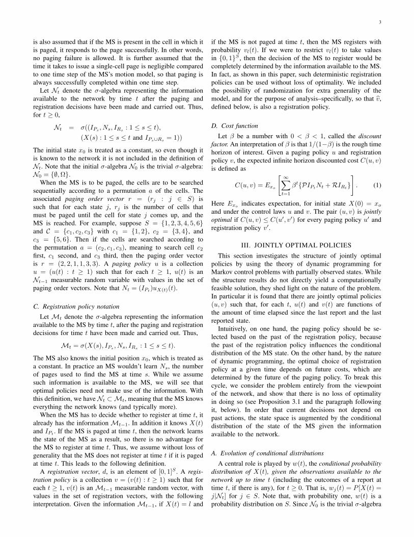
Fig. 1. Paging policy and registration policy generation

cies are threshold policies and the thresholds depend on theMS motion activities. In [14], dynamic programming is used todetermine an optimal state-based registration policy. Work in[2] considers congestion among paging requests for multipleMSs, and considers overlapping registration regions.

Basic paging policies can be classified as follows:• Serial Paging. The cellular network pages the MS se-

quentially, one cell at a time.• Parallel Paging. The cellular network pages the MS in a

collection of cells simultaneously.Serial paging policies have lower paging costs than parallelpaging policies, but at the expense of larger delay. The methodof parallel paging is to partition the cells in a service regioninto a series of indexed groups referred to as paging areas.When a call arrives for the MS, the cells in the first pagingarea are paged simultaneously in the first round and then, if theMS is not found in the first round of paging, all the cells in thesecond paging area are paged, and so on. Given disjoint pagingareas, searching them in the order of decreasing probabilitiesminimizes the the expected number of searches [20]. Thispaging order is denoted as the maximum-likelihood serialpaging order. An interesting topic of paging is to design theoptimal paging areas within delay constraints [20], [12], [23].However, in this paper, we consider only serial paging polices.

Each paper mentioned above assumes a certain class ofpaging or registration policy. Given one policy (paging policyor registration policy) and the parameters of an assumedmotion model, the counterpart policy (registration policy orpaging policy, respectively) is found. For instance, the optimal

2

paging policy is identified in [20] for a given registrationpolicy. This is shown as the top branch of Figure 1. Conversely,an expanding “ping-pong” order paging policy suited to thegiven motion model is assumed in [14]. With this knowledge,dynamic programming is applied to solve for the optimalregistration policy. This corresponds to the bottom branch ofFigure 1.

Several studies have addressed minimizing the costs, con-sidering the paging and registration policies together [21],[1], [22]. In [21], a timer-based registration policy combinedwith maximum-likelihood serial paging is introduced. Theminimum paging cost can be represented by the distribution oflocations where the MS last reported. Then an optimal timerthreshold is selected to minimize the total cost of registrationand paging. By contrast, a movement-based registration policyis used in [1]. An improvement of [21] is given in [22] byassuming that the MS knows not only the current time, butalso its own state and the conditional distribution of its stategiven the last report. This is a state-based registration policyand is aimed to minimize the total costs by running a greedyalgorithm on the potential costs. Although the papers discussthe paging and registration policy together, they don’t considerjointly optimizing the policies.

In our model we assume that when the network pages theMS in a cell in which the MS is located, it is successful withprobability one. At the expense of increasing complexity, wecould have included a known, cell dependent probability ofmissed pages in our model. The work [18] addresses optimalsequential paging with paging misses, in a context with nomobility modeling.

The contributions of this paper are as follows.1 The structureof jointly optimal paging and registration policies is identified.It is shown that the conditional probability distribution ofthe states of an MS can be viewed as a controlled Markovprocess, controlled by both the paging and registration policesat each time. Dynamic programming is applied to show thatthe jointly optimal policies can be represented compactly bycertain reduced complexity laws (RCLs). An iterative algo-rithm producing a pair of RCLs is proposed based on closingthe loop in Figure 1. The algorithm is a heuristic which mergesthe approaches in [14] and [20]. Several examples are given.The first example is an illustration of numerical computationof an individually optimal policy pair. The second example isa simple one illustrating that individually optimal policies arenot necessarily jointly optimal. Finally, three more examplesare given based on random walk models of motion. Majoriza-tion theory and Riesz’s rearrangement inequality are used toshow that jointly optimal paging and registration policies aregiven for these random walk models by the nearest-location-first paging policy and distance threshold registration policies.

The paper is organized as follows. Notation and cost func-tions are introduced in Section II. Jointly optimal policies areinvestigated in Section III. The iterative optimization formulafor computing individually optimal policy pairs is developedin Section IV. The first two examples are given in SectionV, and the random walk examples are given in Section VI.

1Earlier versions of this work appeared in [11], [10].

Conclusions are given in Section VII. The appendix includesa list of notation, a review of σ-algebras, and some proofs.

II. NETWORK MODEL

A. State description and cost

A cell c is a physical location that the MS can be in.Let C denote the set of cells, which is assumed to be finite.The motion of an MS is modeled by a discrete-time Markovprocess (X(t) : t ≥ 0) with a finite state space S, one-step transition probability matrix P = (pij : i, j ∈ S), andinitial state x0. A state j ∈ S determines the cell c that theMS is physically located in, and it may indicate additionalinformation, such as the current velocity of the MS, or thepreviously visited cell. Thus a cell c can be considered to be aset of one or more states, and the set C of all cells is a partitionof S. It is assumed that the network knows the initial state x0.In the special case that there is one state per cell, we writeC = S, and then the MS moves among the cells according toa Markov process.

The possible events at a particular integer time instant t ≥ 1are as follows, listed in the order that they can occur. First,the state X(t) is generated based on X(t − 1) and the one-step transition probability matrix P . Then, with probabilityλp, independently of the state of the MS and all past events,the MS is paged, due to a request from outside the network.The cost of the paging at time t is PNt, where P is thecost of searching one cell and Nt is the number of cells thatare searched until the MS is found. If the MS is paged, thecellular network learns the state, X(t). If the MS is not pagedat time t, let Nt = 0. Finally, if the MS was not paged, theMS decides whether to register. The cost of registration isR and the benefit of registration is that the cellular networklearns the state of the MS. Let Pt denote the event that theMS is paged at time t, and let Rt denote the event that theMS registers at time t. We sometimes use s, instead of t, todenote a discrete time instant. Thus, just as Pt is the event theMS registers at time t, Ps is the event that the MS registersat time s. No paging or registration is considered for t = 0,and we set P0 = R0 = ∅ and N0 = 0.

We say that a report occurs at time t if either a pagingor a registration occurs, because in either case, the cellularnetwork learns the state of the MS. For any set A, let IAdenote the indicator function of A, which is one on A andzero on the complement, Ac. Discrete probability distributionsare considered to be row vectors. Given a state l ∈ S, letδ(l) denote the probability distribution on S which assignsprobability one to state l. Thus, δi(l) = Ii=l. A key aspect ofthe model and analysis is to specify the information availableto the MS and to the network. For this purpose we use thenotion of a σ-algebra to model the information that is availableto a given decision maker at a given time. For the reader’sconvenience, the definitions of σ-algebras and the propertieswe use are reviewed in the appendix.

B. Paging policy notation

For simplicity we consider only serial paging policies, sothat cells are searched one at a time until the MS is located. It

3

is also assumed that if the MS is present in the cell in which itis paged, it responds to the page successfully. In other words,no paging failure is allowed. It is further assumed that thetime it takes to issue a single-cell page is negligible comparedto one time step of the MS’s motion model, so that paging isalways successfully completed within one time step.

Let Nt denote the σ-algebra representing the informationavailable to the network by time t after the paging andregistration decisions have been made and carried out. Thus,for t ≥ 0,

Nt = σ((IPs , Ns, IRs : 1 ≤ s ≤ t),(X(s) : 1 ≤ s ≤ t and IPs∪Rs = 1))

The initial state x0 is treated as a constant, so even though itis known to the network it is not included in the definition ofNt. Note that the initial σ-algebra N0 is the trivial σ-algebra:N0 = ∅,Ω.

When the MS is to be paged, the cells are to be searchedsequentially according to a permutation a of the cells. Theassociated paging order vector r = (rj : j ∈ S) issuch that for each state j, rj is the number of cells thatmust be paged until the cell for state j comes up, and theMS is reached. For example, suppose S = 1, 2, 3, 4, 5, 6and C = c1, c2, c3 with c1 = 1, 2, c2 = 3, 4, andc3 = 5, 6. Then if the cells are searched according tothe permutation a = (c2, c1, c3), meaning to search cell c2first, c1 second, and c3 third, then the paging order vectoris r = (2, 2, 1, 1, 3, 3). A paging policy u is a collectionu = (u(t) : t ≥ 1) such that for each t ≥ 1, u(t) is anNt−1 measurable random variable with values in the set ofpaging order vectors. Note that Nt = (IPt)uX(t)(t).

C. Registration policy notation

Let Mt denote the σ-algebra representing the informationavailable to the MS by time t, after the paging and registrationdecisions for time t have been made and carried out. Thus,

Mt = σ(X(s), IPs , Ns, IRs : 1 ≤ s ≤ t).

The MS also knows the initial position x0, which is treated asa constant. In practice an MS wouldn’t learn Ns, the numberof pages used to find the MS at time s. While we assumesuch information is available to the MS, we will see thatoptimal policies need not make use of the information. Withthis definition, we haveNt ⊂Mt, meaning that the MS knowseverything the network knows (and typically more).

When the MS has to decide whether to register at time t, italready has the information Mt−1. In addition it knows X(t)and IPt . If the MS is paged at time t, then the network learnsthe state of the MS as a result, so there is no advantage forthe MS to register at time t. Thus, we assume without loss ofgenerality that the MS does not register at time t if it is pagedat time t. This leads to the following definition.

A registration vector, d, is an element of [0, 1]S . A regis-tration policy is a collection v = (v(t) : t ≥ 1) such that foreach t ≥ 1, v(t) is an Mt−1 measurable random vector, withvalues in the set of registration vectors, with the followinginterpretation. Given the information Mt−1, if X(t) = l and

if the MS is not paged at time t, then the MS registers withprobability vl(t). If we were to restrict vl(t) to take valuesin 0, 1S , then the decision of the MS to register would becompletely determined by the information available to the MS.In fact, as shown in this paper, such deterministic registrationpolicies can be used without loss of optimality. We includedthe possibility of randomization for extra generality of themodel, and for the purpose of analysis–specifically, so that v,defined below, is also a registration policy.

D. Cost function

Let β be a number with 0 < β < 1, called the discountfactor. An interpretation of β is that 1/(1−β) is the rough timehorizon of interest. Given a paging policy u and registrationpolicy v, the expected infinite horizon discounted cost C(u, v)is defined as

C(u, v) = Exo

[ ∞∑t=1

βtPIPtNt +RIRt

]. (1)

Here Exo indicates expectation, for initial state X(0) = xoand under the control laws u and v. The pair (u, v) is jointlyoptimal if C(u, v) ≤ C(u′, v′) for every paging policy u′ andregistration policy v′.

III. JOINTLY OPTIMAL POLICIES

This section investigates the structure of jointly optimalpolicies by using the theory of dynamic programming forMarkov control problems with partially observed states. Whilethe structure results do not directly yield a computationallyfeasible solution, they shed light on the nature of the problem.In particular it is found that there are jointly optimal policies(u, v) such that, for each t, u(t) and v(t) are functions ofthe amount of time elapsed since the last report and the lastreported state.

Intuitively, on one hand, the paging policy should be se-lected based on the past of the registration policy, becausethe past of the registration policy influences the conditionaldistribution of the MS state. On the other hand, by the natureof dynamic programming, the optimal choice of registrationpolicy at a given time depends on future costs, which aredetermined by the future of the paging policy. To break thiscycle, we consider the problem entirely from the viewpointof the network, and show that there is no loss of optimalityin doing so (see Proposition 3.1 and the paragraph followingit, below). In order that current decisions not depend onpast actions, the state space is augmented by the conditionaldistribution of the state of the MS given the informationavailable to the network.

A. Evolution of conditional distributions

A central role is played by w(t), the conditional probabilitydistribution of X(t), given the observations available to thenetwork up to time t (including the outcomes of a report attime t, if there is any), for t ≥ 0. That is, wj(t) = P [X(t) =j|Nt] for j ∈ S. Note that, with probability one, w(t) is aprobability distribution on S. Since N0 is the trivial σ-algebra

4

and X(0) = x0, the initial conditional distribution is given byw(0) = δ(x0).

While the network may not know the recent past trajectoryof the state process, it can still estimate the registration prob-abilities used by the MS. In particular, as shown in the nextlemma, the estimate vj(t), defined by vj(t) = E[vj(t)|X(t) =j,Nt−1], plays a role in how the network can recursivelyupdate the w(t)’s. In more conventional notation, we have

vj(t) =E[vj(t)IX(t)=j|Nt−1]P [X(t) = j|Nt−1]

.

Define a function Φ as follows. Let w be a probabilitydistribution on S and let d be a registration vector, i.e.,d ∈ [0, 1]S . Let Φ(w, d) denote the probability distributionon S defined by

Φl(w, d) =

∑j∈S wjpjl(1− dl)∑

l′∈S∑j∈S wjpjl′(1− dl′)

.

Φ(w, d) is undefined if the denominator in this definition iszero. The meaning of Φ is that if at time t the network knowsthat X(t) has distribution w, if no paging occurs at time t+1,and if the MS registers at time t+ 1 with probability dX(t+1),then Φ(w, d) is the conditional distribution of X(t+ 1) givenno registration occurs at time t+1. This interpretation is madeprecise in the next lemma. The proof is in the appendix.

Lemma 3.1: The following holds, under the paging andregistration policies u and v:

w(t+ 1) = δ(X(t+ 1))IPt+1∪Rt+1 (2)+Φ(w(t), v(t+ 1))IP ct+1∩Rct+1

.

The first term on the right hand side of (2) indicates thatif there is a report at time t + 1, then the network learnsthe value of X(t + 1), so the conditional distribution w(t +1) is concentrated on the single state X(t + 1). The secondterm gives the update, according to the one step transitionprobabilities and Bayes rule, of the conditional distribution ofX(t + 1), based on w(t) and what can be estimated aboutv(t+ 1).

B. New state process

Define a new random process (Θ(t) : t ≥ 0), by Θ(t) =(w(t), IPt , Nt, IRt). Note that the tth term in the cost functionis a function of Θ(t). Note also that Θ(t) is measurablewith respect to Nt, so that the network can calculate Θ(t)at time t (after possible paging and registration). Moreover,the first coordinate of Θ(t), namely w(t), can be updatedfor increasing t with the help of Lemma 3.1. The randomprocess (Θ(t) : t ≥ 0) can be viewed as a controlled Markovprocess, adapted to the family of σ-algebras (Nt : t ≥ 0)with controls (u(t), v(t) : t ≥ 1). Note that u(t + 1) andv(t + 1) are each Nt measurable for each t ≥ 0. The inititalvalue is Θ(0) = (δ(xo), 0, 0, 0). The conditional distributionof Θ(t+1) given Θ(t), u(t+1) and v(t+1) is given as follows,where the variables j and l range over the set of states S:

Θ(t+ 1) probability

(δ(l), 1, ul(t+ 1), 0) λp

Pj wj(t)pjl

(δ(l), 0, 0, 1) (1− λp)P

j wj(t)pjlbvl(t+ 1)

(Φ(w(t), bv(t+ 1)), 0, 0, 0) (1− λp)P

j wj(t)pjl(1− bvl(t+ 1))

Observe that although the MS uses a registration policyv, the one-step transition probabilities for Θ depend only onv. Moreover, v is itself a registration policy. Indeed, sinceNt−1 ⊂Mt−1, v(t) is Mt−1 measurable, and it takes valuesin [0, 1]S . If v were used instead of v as a registration policyby the MS, the one-step transition probabilities for Θ wouldbe unchanged. Thus, the policy v is adapted to the family ofσ algebras (Nt : t ≥ 0), and it yields the same cost as v.Therefore, without loss of generality, we can restrict attentionto registration policies v that are adapted to (Nt : t ≥ 0).

Combining the observations summarized in this section, wearrive at the following proposition.

Proposition 3.1: The original joint optimization problem isequivalent to a Markov optimal control problem with stateprocess (Θ(t) : t ≥ 0) adapted to the family of σ-algebras(Nt : t ≥ 0), with controls (u(t), v(t) : t ≥ 1).

We remark that one can think of the Markov control problemmentioned in Proposition 3.1 as one faced by the network,because both controls u and v are based on informationavailable to the network. The network does not know X(t), butwe can view the network as controlling Θ(t) (and in particularw(t)) through an optimal choice of u and v.

C. Dynamic programming equations

Above it was assumed that w(0) = δ(x0), where x0 isthe initial state of the MS, assumed known by the network.In order to apply the dynamic programming technique, inthis section the initial distribution w(0) is allowed to be anyprobability distribution on S. It is assumed that the networkknows w(0) at time zero, and that the initial state of the MS israndom, with distribution w(0). The evolution of the systemas described in the previous section is well defined for anarbitrary initial distribution w(0). Let Ew denote conditionalexpectation in case the initial distribution w(0) is taken tobe w. The initial σ-algebra N0 is still the trivial σ-algebra,because w(0) is treated as a given constant.

Define the cost with n steps to go as

Un(w) = minu,bv Ew[

n∑t=1

βtPIPtNt +RIRt]

Here we have expressed the cost-to-go as a function of walone, rather than as a function of the complete state, becausethe conditional distribution of Θ(t+1) given Θ(t) depends onΘ(t) only through w(t). Next apply the backwards solutionmethod of dynamic programming, by separating out the t = 1

5

term in the cost for n+ 1 steps to go. This yields

Un+1(w) = minu,bv β

λpP∑j

∑l

wjpjlul(1)

+(1− λp)R∑j

∑l

wjpjlvl(1)

+Ew[Ew[n+1∑t=2

βt−1PIPtNt +RIRt|N1]]

]Note that u(1) and v(1) are both measurable with respectto the trivial σ-algebra N0. Therefore these controls areconstants. Henceforth we write d for the registration decisionvector v(1). The vector d ranges over the space [0, 1]S .

The first sum in the expression for Un+1(w) involves thecontrol policies only through the choice of the paging ordervector u(1). This sum is simply the mean number of single-cell pages required to find the MS given that the state of theMS has distribution given by the product wP , where P is thematrix of state transition probabilities. It is well known thatthe optimal search order is to first search the cell with thelargest probability, then search the cell with the second largestprobability, and so on [20]. Ties can be broken arbitrarily. Thefirst sum in the expression for Un+1(w) can thus be replacedby s(wP ), where, for a probability distribution µ on S, s(µ)denotes the mean number of single cell pages required to findthe MS given that the state of the MS has distribution µ and theoptimal paging policy is used. Following [8], we call s(µ) theguessing entropy of µ. We remark that Massey [17] exploredcomparisons between s(µ), in the case of one state per cell,and the ordinary entropy, H(µ) =

∑i µi logµi. Later work

(see [9]) compares guessing entropy to other forms of entropy.The dynamic programming equation thus becomes

Un+1(w) = βλpPs(wP )

mindβ

∑j

∑l

wjpjl λpUn(δ(l))

+(1− λp)dl(R+ Un(δ(l)))

+ (1− λp)

∑j

∑l

wjpjl(1− dl)

Un(Φ(w, d))

.(3)

Formally we denote this equation as Un+1 = T (Un). By astandard argument for dynamic programming with discountedcost, T has the following contraction property:

supw|T (U)− T (U ′)| ≤ β sup

w|U − U ′| (4)

for any bounded, measurable functions U and U ′, defined onthe space of all probability distributions w on S. Consequently[5], [6], there exists a unique U∗ such that T (U∗) = U∗,and Un → U∗ uniformly as n → ∞. Moreover, U∗ isthe minimum possible cost, and a jointly optimal pair ofpaging and registration policies is given by a pair (f , g)of state feedback controls, for the state process (w(t)). Ajointly optimal control is given by u(t) = f(w(t − 1))and v(t) = g(w(t − 1)), where f and g are determined asfollows. For any probability distribution w on S, f(w) is the

paging order vector for paging the cells in order of decreasingprobability under distribution wP , and g(w) is a value of dthat achieves the minimum in the right hand side of (3) withUn replaced by U∗. Then if there is no report at time t + 1,the conditional distribution w(t) is updated simply by:

w(t+ 1) = Φ(w(t), g(w(t))) (5)

Clearly under such stationary state feedback control laws(f , g), the process (w(t) : t ≥ 0) is a time-homogeneousMarkov process. Note that the optimal mapping f does notdepend on g.

Lemma 3.2: The registration policy g can be taken to be0, 1S valued (rather than [0, 1]S valued) without loss ofoptimality.

Proof: It is first proved that Un is concave for any givenn ≥ 0. Suppose w1 and w2 are two probability distributionson S, suppose 0 < η < 1 and suppose w = ηw1 + (1 −η)w2. Then Un(w) can be viewed as the cost to go given theMS has distribution w1 with probability η and distribution w2

with probability 1− η, and the network does not know whichdistribution is used. The sum ηUn(w1) + (1− η)Un(w2) hasa similar interpretation, except the network does know whichdistribution is used. Thus, the sum is less than or equal toUn(w), so that Un is concave. Therefore U∗ is also concave.

Given a function H defined on the space of all probabilitydistributions on S, let H be an extension of H defined onthe positive quadrant RS+ as follows. For any probabilitydistribution w and any constant c ≥ 0, H(cw) = cH(w).It is easy to show that if H is concave then the extension His also concave. With this notation, the dynamic programmingequation for U∗ can be written as:

U∗(w) = βλpPs(wP )

mindβ

∑j

∑l

wjpjl λpU∗(δ(l))

+(1− λp)dl(R+ U∗(δ(l)))+ (1− λp)U∗(wPdiag(1− d))

].

where diag(1−d) is the diagonal matrix with lth entry 1−dl.The expression to be minimized over d in this equation is aconcave function of d, and hence the minimum of the functionoccurs at one of the extreme points of [0, 1]S , which are justthe binary vectors 0, 1S . The minimizing d is g(w). Thiscompletes the proof of the lemma.

D. Reduced complexity laws

Given a pair of feedback controls (f , g), a more compactrepresentation of the controls is possible. The basic idea is thatthe network receives no observations between reports, so theoptimal controls between reports can be precomputed. Indeed,suppose the controls are used, and suppose in addition thatX(0) = x0, where x0 is an initial state known to the network.Given t ≥ 1, define k ≥ 1 and i0 ∈ S as follows. If there wasa report before time t, let t− k be the time of the last reportbefore t. If there was no report before time t let k = t. In eithercase, let i0 = X(t−k). Since the network knows X(t−k) attime t−k (after possible paging or registration), we have that

6

w(t − k) = δ(i0). Since there were no state updates duringthe times t− k + 1, . . . , t− 1, it follows that w(t− 1) is theresult of applying the update (5) k − 1 times, beginning withδ(i0). Hence, w(t− 1) is a function of i0, k. Moreover, sinceu(t) = f(w(t − 1)) and v(t) = g(w(t − 1)), it follows thatboth the paging order vector u(t) and the registration decisionvector v(t) are determined by i0 and k. Let f and g denote themappings such that u(t) = f(i0, k) and v(t) = g(i0, k). Notethat f(i0, k) is a paging order vector and g(i0, k) ∈ 0, 1Sfor each i0, k. We call the mappings f , g reduced complexitylaws (RCLs). We have the following proposition.

Proposition 3.2: There is no loss in optimality for theoriginal joint paging and registration problem to use policiesbased on RCLs.

Proof: By the dynamic programming formulation, thereexist optimal controls for the original paging and registrationproblem which can be expressed using a pair of feedbackcontrols, (f, g). As just described, given (f, g), a pair ofRCLs (f, g) can be found so that f(w(t − 1)) = f(io, k)and g(w(t− 1)) = g(io, k), for all t, with io and k dependingon t as described above. That is, (f, g) produces the samedecisions and therefore the same sample paths as (f, g), andso achieves the same infinite horizon average cost as (f, g),and is thus also optimal.

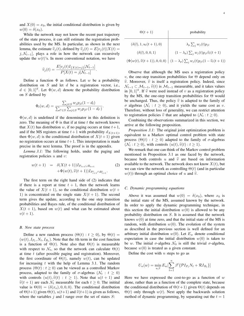
Figure 2 shows an example of a registration RCL g for athree-state Markov chain. The augmented state of the MS isa triple (i0, k, j), such that i0 is the state at the time of thelast report, k is the elapsed time since the last report, and jis the current state. Augmented states marked with an “×”are those for which gj(i0, k) = 1, meaning that registrationoccurs (if paging doesn’t occur first). An MS traverses a pathfrom left to right until either it is paged, or until it hits astate marked with an “×,” at which time its augmented stateinstantaneously jumps. The figure shows the path of a MSthat began in augmented state (i0, k, j) = (2, 0, 2). At relativetime k = 5 the MS entered state 3, hitting an “×”, causingthe extended state to instantly change to (3, 0, 3). Three timeunits after that, upon entering state 1, the MS is paged. Thiscauses the augmented state to instantly jump to (1, 0, 1).

IV. ITERATIVE ALGORITHM FOR FINDINGINDIVIDUALLY OPTIMAL POLICIES

A. Overview of iterative optimization formulationWhile jointly optimal policies can be efficiently represented

by RCLs f and g, the dynamic programming method describedfor finding the optimal policies is far from computationallyfeasible, even for small state spaces, because functions ofdistributions on the state space must be considered. In thissection we explore the following method for finding a pair ofpolicies with a certain local optimality property. First it is showhow to find, for a given paging RCL f , an optimal registrationRCL g. Then it is shown how to find, for a given registrationRCL g, an optimal paging RCL f . Iterating between thesetwo optimization problems produces a pair of RCLs (f, g)such that for each RCL fixed, the other is optimal. Such pairsof RCLs are said to be individually optimal.

In this section we impose the constraint that an MS mustregister if k ≥ kmax, for some large integer constant kmax.

0 1 2 3 4 5 6

path of MS

P

MS is paged

j

1

3

2

1

1

2

2

3

3

3

i = 0 1

i = 0

i = 0

2

3

MS registers

State

Time since last report k

Fig. 2. Example of a registration policy represented by an RCL for a three-state Markov chain

With this constraint, the sets of possible registration andpaging RCLs are finite, and numerical computation is feasiblefor fairly large state spaces. The initial state x0 is assumedto be known and we write C(f, g) for the average infinitehorizon, discounted cost, for paging RCL f and registrationRCL g.

B. Optimal registration RCL for given paging RCL

Suppose a paging RCL f is fixed. In this subsection weaddress the problem of finding a registration RCL g thatminimizes C(f, g) with respect to g. Dynamic programmingis again used, but here the viewpoint of the MS is taken. Thestates used for dynamic programming in this section are theaugmented states of the form (i0, k, j), rather than the set ofall probability distributions on S.

Since time is implicitly included in the variable k in the aug-mented state, it is computationally more efficient to considerdynamic programming iterations based on report cycles ratherthan on single time steps, where each report cycle ends whenthere is a report. Let τm be the time of the mth report. Timeconverges to infinity as the number of report cycles convergesto infinity, so by the monotone convergence theorem,

C(f, g) = limm→∞

E

[τm∑t=1

βt PIPtNt +RIRt

].

Then for each (i0, j, k), write Vm(i0, k, j) for the cost-to-gofor m ≥ 1 report cycles:

Vm(i0, k, j) = minuE

[τm∑t=1

βt PIPtNt +RIRt

], (6)

where the expectation E is taken assuming that (a) the pagingRCL f is used for the paging policy, (b) at t = 0 the MS isin state j, and (c) the last report occurred k time units earlier(i.e., at time −k) in state i0. Also, define V0(i0, k, j) ≡ 0,because the cost is zero when there are no report cycles to go.

7

The dynamic programming optimality equations are givenby

Vm(i0, k, j) = β∑l∈S

pjl [λp(Pfl(i0, k + 1) + Vm−1(l, 0, l))

+ (1− λp) min Vm(i0, k + 1, l),R+ Vm−1(l, 0, l)] (7)

As mentioned earlier, registration is forced at relative timek = kmax + 1 for some large but fixed value kmax. Thereforewe set Vm(i0, kmax + 1, l) = ∞ and use (7) only for0 ≤ k ≤ kmax. These equations represent the basic dynamicprogramming optimality relations. For each possible nextstate, the MS chooses whichever action has lesser cost: eithercontinuing the current registration cycle or registering for costR.

Equation (7) can be used to compute the functions Vmsequentially in m as follows. The initial conditions are V0 ≡ 0.Once Vm−1 is computed, the values Vm(i0, k, j) can be com-puted using (7), sequentially for k decreasing from kmax to 0.Formally we denote this computation as Vm = T (Vm−1). Themapping T is a contraction with constant β in the sup norm,so that Vm converges uniformly to a function V∗ satisfying thelimiting form of (7):

V∗(i0, k, j) = β∑l∈S

pjl [λp(Pfl(i0, k + 1) + V∗(l, 0, l))

+ (1− λp) min V∗(i0, k + 1, l),R+ V∗(l, 0, l)] (8)

for 0 ≤ k ≤ kmax, and V∗(i0, kmax + 1, l) ≡ ∞. Thecorresponding optimal registration RCL g∗ is given by

g∗l (i0, k) =

0, if V∗(i0, k + 1, l) ≤ R+ V∗(l, 0, l)1, else. (9)

for i0 ∈ S and 1 ≤ k ≤ kmax.Thus, for a given paging RCL f , we have identified how to

compute a registration RCL g to minimize C(f, g).

C. Optimal paging RCL for given registration RCL

Suppose a registration RCL g is fixed. In this subsection weaddress the problem of finding a paging RCL f to minimizeC(f, g). For i0 ∈ S and 0 ≤ k ≤ kmax, let w(i0, k) denotethe conditional probability distribution of the state of the MS,given that the most recent report occurred k time units earlierand the state at the time of the most recent report was i0. Thus,w(i0, 0) = δ(i0), and for larger k the w’s can be computedby the recursion:

w(i0, k + 1) = Φ(w(i0, k), g(i0, k))

The paging order vector f(i0, k) is simply the one to be usedwhen the MS must be paged k time units after the previousreport. At such time the conditional distribution of the state ofthe MS given the observations of the base station is w(i0, k−1)P . Thus, the probability the MS is located in cell c, justbefore the paging begins, is given by

p(c|i0, k) =∑j∈S

∑l∈c

wj(i0, k − 1)pjl

Finally, f(i0, k) is the paging order vector for ordering thecells c according to decreasing values of the probabilitiesp(c|i0, k).

i

j

(0,0) (4,0)

(0,4)

(2,2)

(4,4)

L R

U

D

CurrentCell

u

d

rl

sty

p

p

pp

p

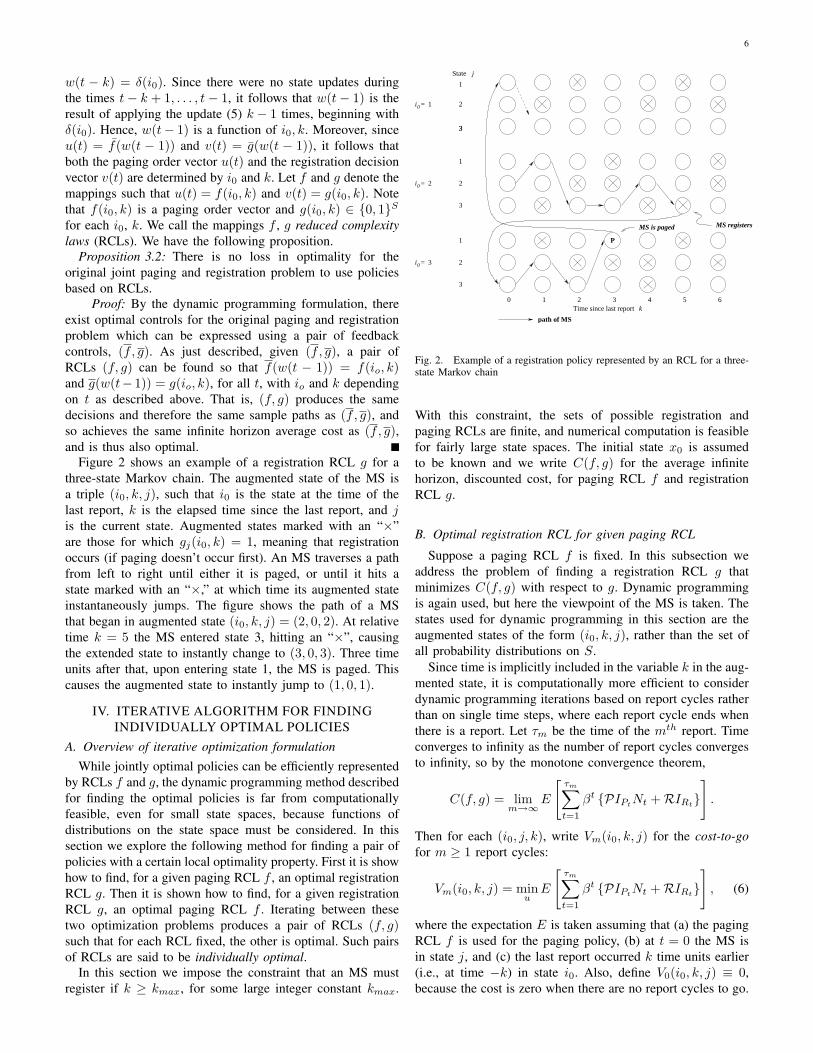
Fig. 3. Rectangular grid motion model

D. Iterative optimization algorithm

In the previous subsections we described how to find anoptimal g for given f and vice versa. This suggests an iterativemethod for finding an individually optimal pair (f, g). Themethod works as follows. Fix an arbitrary registration RCLg0. Then execute the following steps.• Find a paging RCL f0 to minimize C(f0, g0)• Find a registration RCL g1 to minimize C(f0, g1),• Find a paging RCL f1 to minimize C(f1, g1), and so on.

Then C(f0, g0) ≥ C(f0, g1) ≥ C(f1, g1) ≥ C(f1, g2) ≥ · · ·Since there are only finitely many RCLs, it must be that forsome integer d, C(fd, gd) = C(fd, gd+1). By construction,the paging RCL fd is optimal given the registration RCLgd. Similarly, gd+1 is optimal given fd. However, sinceC(fd, gd) = C(fd, gd+1), it follows that gd is also optimalgiven the registration RCL fd. Therefore, (fd, gd) is anindividually optimal pair of RCLs.

V. EXAMPLES

Two examples illustrating individually optimal RCLs aregiven in this section. Examples of jointly optimal policies forrandom walk models are given in the next section.

A. Rectangular grid example

Consider a rectangular grid topology, such that each cell hasfour neighbors. The diagram to the left in Figure 3 shows thefinite imax × jmax rectangular grid topology. To provide thefull complement of four neighbors to cells on the edges of thegrid, the region is wrapped into a torus. The torus can serve toapproximate larger sets of cells. Also, by the symmetry of thetorus, the functions f(i0, k), g(i0, k) and distributions w(i0, k)need be computed for only one value of last reported cell i0.Each cell in Figure 3 is represented by the index pair (i, j),where i = 0, 1, . . . , imax − 1 is the index for the horizontalaxis, and j = 0, 1, . . . , jmax − 1 is the index for the verticalaxis.

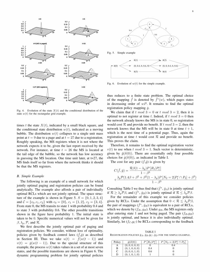
For simplicity, we assume that there is only one state percell, so we can take C = S. For a numerical example, considera 15×15 torus grid with motion parameters psty = 0.4, pu =pd = pl = 0.1, pr = 0.3, x0 = (5, 5) and other parametersλp = 0.03, P = 1, R = 0.6, β = 0.9, and kmax = 200.We numerically calculated an individually optimal pair (f, g)of RCLs. A sample path of X and w generated using thosecontrols is indicated in Figure 4. The figure shows for selected

8

t=0

010

0

1000.20.40.60.8

1

t=0

010

0

1000.20.40.60.8

1

t=5

010

0

100

0.05

0.1

0.15

0.2

t=5

010

0

100

0.05

0.1

0.15

0.2

t=9 (MS is paged)

010

0

1000.20.40.60.8

1

t=9 (MS is paged)

010

0

1000.20.40.60.8

1

t=16

010

0

100

0.05

0.1

0.15

0.2

t=16

010

0

100

0.05

0.1

0.15

0.2

t=20

010

0

100

0.05

0.1

0.15

0.2

t=20

010

0

100

0.05

0.1

0.15

0.2

t=26

010

0

100

0.05

0.1

0.15

0.2

t=26

010

0

100

0.05

0.1

0.15

0.2

t=27 (MS registers)

010

0

1000.20.40.60.8

1

t=27 (MS registers)

010

0

1000.20.40.60.8

1

t=33

010

0

100

0.05

0.1

0.15

0.2

t=33

010

0

100

0.05

0.1

0.15

0.2

Fig. 4. Evolution of the state X(t) and the conditional distribution of thestate w(t) for the rectangular grid example.

times t the state X(t), indicated by a small black square, andthe conditional state distribution w(t), indicated as a movingbubble. The distribution w(t) collapses to a single unit masspoint at t = 9 due to a page and at t = 27 due to a registration.Roughly speaking, the MS registers when it is not where thenetwork expects it to be, given the last report received by thenetwork. For instance, at time t = 26 the MS is located atthe tail edge of the bubble, so the network has low accuracyin guessing the MS location. One time unit later, at t=27, theMS finds itself so far from where the network thinks it shouldbe that the MS registers.

B. Simple Example

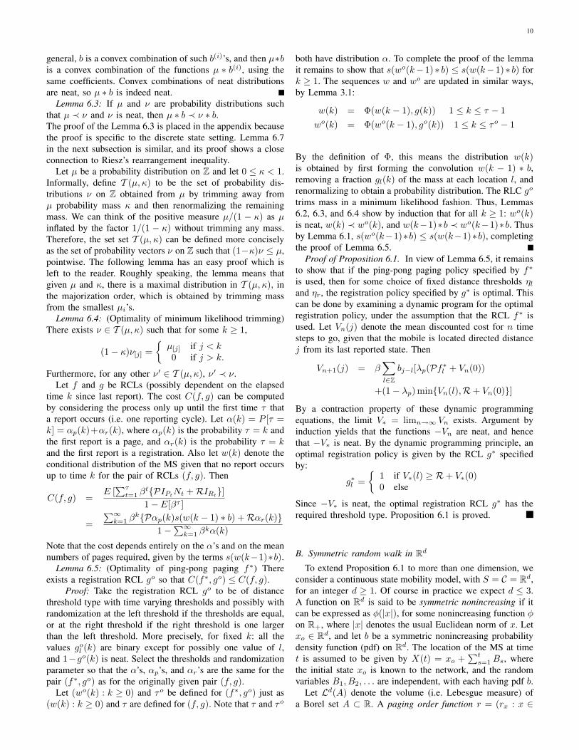
The following is an example of a small network for whichjointly optimal paging and registration policies can be foundanalytically. The example also affords a pair of individuallyoptimal RCLs which are not jointly optimal. The space struc-ture of the example is shown in Figure 5. S = 0, 1, 2, 3, 4and C = c0, c1, c2 with c0 = 0, c1 = 1, 2, c2 = 3, 4.From state 0, the MS transits to state 1 with probability 0.4 andto state 3 with probability 0.6. The other possible transitionsshown in the figure have probability 1. The initial state istaken to be 0. Specific numerical values will not be given forβ, λp,P , and R.

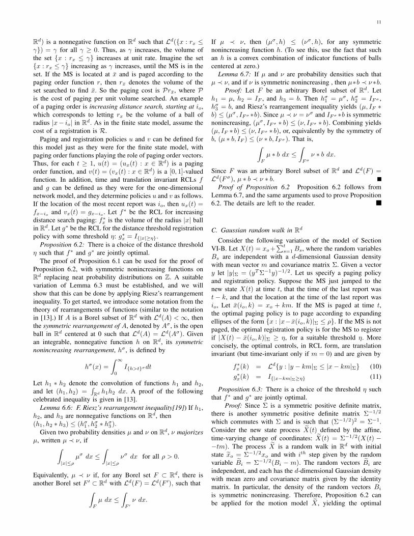
We first describe the jointly optimal pair of paging andregistration policies. We consider, without loss of optimality,policies given by feedback control laws (f ,g) as describedin Section III. Thus we take u(t) = f(w(t − 1)) andv(t) = g(w(t − 1)). Due to the special structure of thisexample, the process w(t) takes values in a set of at most sevenstates, and the possible transitions are shown in Figure 6. Thedynamic programming problem for jointly optimal policies

0

1

2 3

4

1 1

1

0.6

C

C

0

1 2C

0.4

1

Fig. 5. Simple example

δ(0)

δ(1)

(0, 0.4, 0, 0.6, 0)

δ(3)

δ(2)

(0, 0, 0.4, 0, 0.6)

δ(4)

Fig. 6. Evolution of w(t) for the simple example.

thus reduces to a finite state problem. The optimal choiceof the mapping f is denoted by f∗(w), which pages statesin decreasing order of wP . It remains to find the optimalregistration policy mapping g.

We claim that if t mod 3 = 0 or t mod 3 = 2, then it isoptimal to not register at time t. Indeed, if t mod 3 = 0 thenthe network already knows the MS is in state 0, so registrationwould cost R and provide no benefit. If t mod 3 = 2, then thenetwork knows that the MS will be in state 0 at time t + 1,which is the next time of a potential page. Thus, again theregistration at time t would cost R and provide no benefit.This proves the claim.

Therefore, it remains to find the optimal registration vectorv(t) to use when t mod 3 = 1. Such vector is deterministic,given by g(δ(0)). There are essentially only four possiblechoices for g(δ(0)), as indicated in Table I.

The cost for any pair (f ,g) is given by

C(f , g) =Rβ(1− λp)P [R1|P c1 ]

1− β3

+λpP(1.4β + β2 + β2(1− λp)P [N2 = 2|P c1 ∩ P2] + β3)

1− β3

Consulting Table I we thus find that (f∗, gA) is jointly optimalif R ≥ λpPβ, and (f∗, gB) is jointly optimal if R ≤ λpPβ.

For the remainder of this example we consider policiesgiven by RCLs. Under the assumption that 0 < R ≤ λpPβ,the pair of mappings (f∗, gB) is equivalent to a pair of RCLs,which we denote by (fB , gB). Under gB , the MS registers onlyafter entering state 1 and not being paged. The pair (fB ,gB)is jointly optimal, and hence it is also individually optimal.Similarly, let (fC ,gC) be RCLs corresponding to the feedback

TABLE IREGISTRATION POLICIES gA , gB ,gC , gD FOR THE SIMPLE EXAMPLE.

Policy g(δ(0)) PˆR1|P c

1

˜P

ˆN2 = 2|P c

1 ∩ P2

˜A (0, 0, 0, 0, 0) 0 0.4B (0, 1, 0, 0, 0) 0.4 0C (0, 0, 0, 1, 0) 0.6 0D (0, 1, 0, 1, 0) 1 0

9

mappings (f∗,gC). In particular, an MS using registration RCLgC registers only after entering state 3 and not being paged.

Proposition 5.1: Assuming 0 < R < λpPβ, the pair ofRCLs (fC ,gC) is individually optimal, but not jointly optimal.

Proof: The paging RCL fC is optimal for the registrationRCL gC because for gC fixed, it is equivalent to the optimalfeedback mapping f∗. Suppose then that the MS uses thepaging RCL fC . Note that if the MS does not report at timet = 1, and if it is paged at time t = 2, the network willpage cell c1 first. Hence, if the MS enters state 3 at timet = 1 and if it is not paged at t = 1, then by registering forcost R it can avoid the two or more pages required at timet = 2 in case of a page at t = 2. Since R < λpPβ, it isoptimal to have the MS register at t = 1 in this situation.Thus gC is optimal for fC , so the pair is individually optimal.However, C(fC , gC) > C(fB , gB), so that (fC , gC) is notjointly optimal.

VI. JOINTLY OPTIMAL POLICIES FOR SOME RANDOMWALK MODELS

The structure of jointly optimal paging and registrationpolicies are identified in this section for three random walkmodels of motion. The first is a discrete state one-dimensionalrandom walk, the second is a symmetric random walk in Rdfor any d ≥ 1, and the third is a Gaussian random walk in Rdfor any d ≥ 1.

A. Symmetric random walk in ZSuppose the motion of the MS is modeled by a discrete-time

random walk on an infinite linear array of cells, such that thedisplacement of the walk at each step has some probabilitydistribution b. Equivalently, (X(t) : t ≥ 0) is a discretetime Markov process on Z with one-step transition probabilitymatrix P given by pij = bj−i. For any probability distributionw, wP = w ∗ b. It is assumed that bi is a nonincreasingfunction of |i|, or in other words, b is symmetric about zero andunimodal. In the general form of our model, multiple statescan correspond to the same cell, but for this example, eachinteger state i corresponds to a distinct cell in which the MScan be paged. So C = S = Z. It is assumed that the networkknows the initial state, x0.

Due to the translation invariance of P for this example,the update equations of the dynamic program are translationinvariant, and therefore the paging and registration RCLs canalso be taken to be translation invariant. Thus, we write theRCLs as f = (f(k) : k ≥ 1) and g = (g(k) : k ≥ 1). TheseRCLs give the control decisions if the last reported state isi0 = 0, and hence for other values of i0 by translation inspace.

It turns out that for this example, the optimal paging policyis ping-pong type: cells are searched in an order of increasingdistance from the cell in which the previous report occurred.The optimal registration policy is a distance threshold type:the mobile station registers whenever its distance from theprevious reporting point exceeds a threshold. Specifically, onlyRCLs of the following form need to be considered. The actionsof the policies do not depend on the time k elapsed since

last report, so the argument k is suppressed. For the pagingpolicy we take the ping-pong policy, given by the RCL f∗ =(0, 1,−1, 2,−2, 3,−3, . . .). Thus, if the MS is to be pagedand if it was last reported to be at state i0, then the states aresearched in the order i0, i0 + 1, i0 − 1, i0 + 2, i0 − 2, . . .. Theregistration policy is given by the RCL g∗l = Il≥ηr or l≤−ηlwhere the two distance thresholds ηl, ηr ≥ 1 are such thateither ηl = ηr or ηl = ηr − 1.

Proposition 6.1: There is a choice of the distance thresh-olds ηl and ηr such that the ping-pong paging policy given byf∗ and the distance-threshold registration policy given by g∗

are jointly optimal.The related work of Madhow, Honig, and Steiglitz [15]

finds the optimal registration policy assuming that the pagingpolicy is fixed to be the ping-pong policy. Also, it is notdifficult to show that for the distance threshold registrationpolicy specified by g∗, the optimal paging policy is the ping-pong paging policy. However, a pair of individually optimalRCLs may not be jointly optimal, as shown in the example ofSection V-B.

The remainder of this section is devoted to the proof ofProposition 6.1. The following notation is standard in thetheory of majorization [16]. Given x = (x1, x2, · · · , xn) ∈Rn, let x↓ denote the nonincreasing rearrangement of x.That is, x↓ = (x[1], x[2], · · · , x[n]), where the coordi-nates x[1], x[2], · · · , x[n] are equal to a rearrangement ofx1, x2, · · · , xn, such that x[1] ≥ x[2] ≥ · · · ≥ x[n]. Giventwo vectors x and y, we say that y majorizes x, denoted byx ≺ y, if the following conditions hold:

q∑i=1

x[i] ≤q∑i=1

y[i] for 1 ≤ q ≤ n− 1

n∑i=1

x[i] =n∑i=1

y[i]

Write x ≡ y to denote that both x ≺ y and y ≺ x, meaningthat y is a rearrangement of x. The relation x ≺ y can bedefined in a similar fashion, in case x and y are nonnegative,summable functions defined on some countably infinite dis-crete set. In such case, x[i] denotes the ith coordinate, whenthe coordinates of x are listed in a nonincreasing order.

The next lemma shows that guessing entropy is montone inthe majorization order:

Lemma 6.1: If µ and ν are probability distributions suchthat µ ≺ ν, then s(µ) ≥ s(ν).

Proof: The lemma follows immediately from the repre-sentation

s(µ) =∞∑i=1

iµ[i] = 1 +∞∑q=1

(1−q∑i=1

µ[i]),

A function or probability distribution µ on Z is said to beneat if µ0 ≥ µ1 ≥ µ−1 ≥ µ2 ≥ µ−2 ≥ . . ..

Lemma 6.2: If µ is a neat probability distribution, then theconvolution µ ∗ b is neat.

Proof: For i ≥ 0, let b(i) denote the uniform probabilitydistribution over the interval of integers [−i, i]. The conclusionis easy to verify in case b has the form b(i) for some i. In

10

general, b is a convex combination of such b(i)’s, and then µ∗bis a convex combination of the functions µ ∗ b(i), using thesame coefficients. Convex combinations of neat distributionsare neat, so µ ∗ b is indeed neat.

Lemma 6.3: If µ and ν are probability distributions suchthat µ ≺ ν and ν is neat, then µ ∗ b ≺ ν ∗ b.The proof of the Lemma 6.3 is placed in the appendix becausethe proof is specific to the discrete state setting. Lemma 6.7in the next subsection is similar, and its proof shows a closeconnection to Riesz’s rearrangement inequality.

Let µ be a probability distribution on Z and let 0 ≤ κ < 1.Informally, define T (µ, κ) to be the set of probability dis-tributions ν on Z obtained from µ by trimming away fromµ probability mass κ and then renormalizing the remainingmass. We can think of the positive measure µ/(1 − κ) as µinflated by the factor 1/(1 − κ) without trimming any mass.Therefore, the set set T (µ, κ) can be defined more conciselyas the set of probability vectors ν on Z such that (1−κ)ν ≤ µ,pointwise. The following lemma has an easy proof which isleft to the reader. Roughly speaking, the lemma means thatgiven µ and κ, there is a maximal distribution in T (µ, κ), inthe majorization order, which is obtained by trimming massfrom the smallest µi’s.

Lemma 6.4: (Optimality of minimum likelihood trimming)There exists ν ∈ T (µ, κ) such that for some k ≥ 1,

(1− κ)ν[j] =µ[j] if j < k0 if j > k.

Furthermore, for any other ν′ ∈ T (µ, κ), ν′ ≺ ν.Let f and g be RCLs (possibly dependent on the elapsed

time k since last report). The cost C(f, g) can be computedby considering the process only up until the first time τ thata report occurs (i.e. one reporting cycle). Let α(k) = P [τ =k] = αp(k)+αr(k), where αp(k) is the probability τ = k andthe first report is a page, and αr(k) is the probability τ = kand the first report is a registration. Also let w(k) denote theconditional distribution of the MS given that no report occursup to time k for the pair of RCLs (f, g). Then

C(f, g) =E [∑τt=1 β

tPIPtNt +RIRt]1− E[βτ ]

=∑∞k=1 β

kPαp(k)s(w(k − 1) ∗ b) +Rαr(k)1−

∑∞k=1 β

kα(k)

Note that the cost depends entirely on the α’s and on the meannumbers of pages required, given by the terms s(w(k−1)∗b).

Lemma 6.5: (Optimality of ping-pong paging f∗) Thereexists a registration RCL go so that C(f∗, go) ≤ C(f, g).

Proof: Take the registration RCL go to be of distancethreshold type with time varying thresholds and possibly withrandomization at the left threshold if the thresholds are equal,or at the right threshold if the right threshold is one largerthan the left threshold. More precisely, for fixed k: all thevalues gol (k) are binary except for possibly one value of l,and 1−go(k) is neat. Select the thresholds and randomizationparameter so that the α’s, αp’s, and αr’s are the same for thepair (f∗, go) as for the originally given pair (f, g).

Let (wo(k) : k ≥ 0) and τo be defined for (f∗, go) just as(w(k) : k ≥ 0) and τ are defined for (f, g). Note that τ and τo

both have distribution α. To complete the proof of the lemmait remains to show that s(wo(k− 1) ∗ b) ≤ s(w(k− 1) ∗ b) fork ≥ 1. The sequences w and wo are updated in similar ways,by Lemma 3.1:

w(k) = Φ(w(k − 1), g(k)) 1 ≤ k ≤ τ − 1wo(k) = Φ(wo(k − 1), go(k)) 1 ≤ k ≤ τo − 1

By the definition of Φ, this means the distribution w(k)is obtained by first forming the convolution w(k − 1) ∗ b,removing a fraction gl(k) of the mass at each location l, andrenormalizing to obtain a probability distribution. The RLC go

trims mass in a minimum likelihood fashion. Thus, Lemmas6.2, 6.3, and 6.4 show by induction that for all k ≥ 1: wo(k)is neat, w(k) ≺ wo(k), and w(k−1)∗b ≺ wo(k−1)∗b. Thusby Lemma 6.1, s(wo(k−1)∗b) ≤ s(w(k−1)∗b), completingthe proof of Lemma 6.5.

Proof of Proposition 6.1. In view of Lemma 6.5, it remainsto show that if the ping-pong paging policy specified by f∗

is used, then for some choice of fixed distance thresholds ηland ηr, the registration policy specified by g∗ is optimal. Thiscan be done by examining a dynamic program for the optimalregistration policy, under the assumption that the RCL f∗ isused. Let Vn(j) denote the mean discounted cost for n timesteps to go, given that the mobile is located directed distancej from its last reported state. Then

Vn+1(j) = β∑l∈Z

bj−l[λp(Pf∗l + Vn(0))

+(1− λp) minVn(l),R+ Vn(0)]

By a contraction property of these dynamic programmingequations, the limit V∗ = limn→∞ Vn exists. Argument byinduction yields that the functions −Vn are neat, and hencethat −V∗ is neat. By the dynamic programming principle, anoptimal registration policy is given by the RCL g∗ specifiedby:

g∗l =

1 if V∗(l) ≥ R+ V∗(0)0 else

Since −V∗ is neat, the optimal registration RCL g∗ has therequired threshold type. Proposition 6.1 is proved.

B. Symmetric random walk in Rd

To extend Proposition 6.1 to more than one dimension, weconsider a continuous state mobility model, with S = C = Rd,for an integer d ≥ 1. Of course in practice we expect d ≤ 3.A function on Rd is said to be symmetric nonincreasing if itcan be expressed as φ(|x|), for some nonincreasing function φon R+, where |x| denotes the usual Euclidean norm of x. Letxo ∈ Rd, and let b be a symmetric nonincreasing probabilitydensity function (pdf) on Rd. The location of the MS at timet is assumed to be given by X(t) = xo +

∑ts=1Bs, where

the initial state xo is known to the network, and the randomvariables B1, B2, . . . are independent, with each having pdf b.

Let Ld(A) denote the volume (i.e. Lebesgue measure) ofa Borel set A ⊂ R. A paging order function r = (rx : x ∈

11

Rd) is a nonnegative function on Rd such that Ld(x : rx ≤γ) = γ for all γ ≥ 0. Thus, as γ increases, the volume ofthe set x : rx ≤ γ increases at unit rate. Imagine the setx : rx ≤ γ increasing as γ increases, until the MS is in theset. If the MS is located at x and is paged according to thepaging order function r, then rx denotes the volume of theset searched to find x. So the paging cost is Prx, where Pis the cost of paging per unit volume searched. An exampleof a paging order is increasing distance search, starting at io,which corresponds to letting rx be the volume of a ball ofradius |x− io| in Rd. As in the finite state model, assume thecost of a registration is R.

Paging and registration policies u and v can be defined forthis model just as they were for the finite state model, withpaging order functions playing the role of paging order vectors.Thus, for each t ≥ 1, u(t) = (ux(t) : x ∈ Rd) is a pagingorder function, and v(t) = (vx(t) : x ∈ Rd) is a [0, 1]-valuedfunction. In addition, time and translation invariant RCLs fand g can be defined as they were for the one-dimensionalnetwork model, and they determine policies u and v as follows.If the location of the most recent report was io, then ux(t) =fx−io and vx(t) = gx−io . Let f∗ be the RCL for increasingdistance search paging: f∗x is the volume of the radius |x| ballin Rd. Let g∗ be the RCL for the distance threshold registrationpolicy with some threshold η: g∗x = I|x|≥η.

Proposition 6.2: There is a choice of the distance thresholdη such that f∗ and g∗ are jointly optimal.

The proof of Proposition 6.1 can be used for the proof ofProposition 6.2, with symmetric nonincreasing functions onRd replacing neat probability distributions on Z. A suitablevariation of Lemma 6.3 must be established, and we willshow that this can be done by applying Riesz’s rearrangementinequality. To get started, we introduce some notation from thetheory of rearrangements of functions (similar to the notationin [13].) If A is a Borel subset of Rd with Ld(A) <∞, thenthe symmetric rearrangement of A, denoted by Aσ , is the openball in Rd centered at 0 such that Ld(A) = Ld(Aσ). Givenan integrable, nonnegative function h on Rd, its symmetricnonincreasing rearrangement, hσ , is defined by

hσ(x) =∫ ∞

0

Ih>tσdt

Let h1 ∗ h2 denote the convolution of functions h1 and h2,and let (h1, h2) =

∫Rd h1h2 dx. A proof of the following

celebrated inequality is given in [13].Lemma 6.6: F. Riesz’s rearrangement inequality[19]) If h1,

h2, and h3 are nonnegative functions on Rd, then(h1, h2 ∗ h3) ≤ (hσ1 , h

σ2 ∗ hσ3 ).

Given two probability densities µ and ν on Rd, ν majorizesµ, written µ ≺ ν, if∫

|x|≤ρµσ dx ≤

∫|x|≤ρ

νσ dx for all ρ > 0.

Equivalently, µ ≺ ν if, for any Borel set F ⊂ Rd, there isanother Borel set F ′ ⊂ Rd with Ld(F ) = Ld(F ′), such that∫

F

µ dx ≤∫F ′ν dx.

If µ ≺ ν, then (µσ, h) ≤ (νσ, h), for any symmetricnonincreasing function h. (To see this, use the fact that suchan h is a convex combination of indicator functions of ballscentered at zero.)

Lemma 6.7: If µ and ν are probability densities such thatµ ≺ ν, and if ν is symmetric nonincreasing , then µ∗b ≺ ν∗b.

Proof: Let F be an arbitrary Borel subset of Rd. Leth1 = µ, h2 = IF , and h3 = b. Then hσ1 = µσ , hσ2 = IFσ ,hσ3 = b, and Riesz’s rearrangement inequality yields (µ, IF ∗b) ≤ (µσ, IFσ ∗b). Since µ ≺ ν = νσ and IFσ ∗b is symmetricnonincreasing, (µσ, IFσ ∗ b) ≤ (ν, IFσ ∗ b). Combining yields(µ, IF ∗ b) ≤ (ν, IFσ ∗ b), or, equivalently by the symmetry ofb, (µ ∗ b, IF ) ≤ (ν ∗ b, IFσ ). That is,∫

F

µ ∗ b dx ≤∫Fσ

ν ∗ b dx.

Since F was an arbitrary Borel subset of Rd and Ld(F ) =Ld(Fσ), µ ∗ b ≺ ν ∗ b.

Proof of Proposition 6.2 Proposition 6.2 follows fromLemma 6.7, and the same arguments used to prove Proposition6.2. The details are left to the reader.

C. Gaussian random walk in Rd

Consider the following variation of the model of SectionVI-B. Let X(t) = xo+

∑ts=1Bs, where the random variables

Bs are independent with a d-dimensional Gaussian densitywith mean vector m and covariance matrix Σ. Given a vectory let |y|Σ = (yTΣ−1y)−1/2. Let us specify a paging policyand registration policy. Suppose the MS just jumped to thenew state X(t) at time t, that the time of the last report wast− k, and that the location at the time of the last report wasio, Let x(io, k) = xo + km. If the MS is paged at time t,the optimal paging policy is to page according to expandingellipses of the form x : |x− x(io, k)|Σ ≤ ρ. If the MS is notpaged, the optimal registration policy is for the MS to registerif |X(t) − x(io, k)|Σ ≥ η, for a suitable threshold η. Moreconcisely, the optimal controls, in RCL form, are translationinvariant (but time-invariant only if m = 0) and are given by

f∗x(k) = Ldy : |y − km|Σ ≤ |x− km|Σ (10)g∗x(k) = I|x−km|Σ≥η (11)

Proposition 6.3: There is a choice of the threshold η suchthat f∗ and g∗ are jointly optimal.

Proof: Since Σ is a symmetric positive definite matrix,there is another symmetric positive definite matrix Σ−1/2

which commutes with Σ and is such that (Σ−1/2)2 = Σ−1.Consider the new state process X(t) defined by the affine,time-varying change of coordinates: X(t) = Σ−1/2(X(t) −−tm). The process X is a random walk in Rd with initialstate xo = Σ−1/2xo and with ith step given by the randomvariable Bi = Σ−1/2(Bi − m). The random vectors Bi areindependent, and each has the d-dimensional Gaussian densitywith mean zero and covariance matrix given by the identitymatrix. In particular, the density of the random vectors Biis symmetric nonincreasing. Therefore, Proposition 6.2 canbe applied for the motion model X , yielding the optimal

12

paging and registration policies in the new coordinates. Sincethe change of coordinates is invertible for a given time t,determining X(t) is the same as determining X(t). Searchinga region A for X(t) is equivalent to searching the regionQ1/2A + mt for X(t), which has cost (det(Q))1/2PLd(A).Therefore, the original paging and registration problem forX is equivalent to the paging and registration problem for X ,with searching cost per unit volume P equal to (det(Q))1/2P .Finally, mapping back the optimal paging and registrationpolicies for X to the orginal coordinates, completes the proofof the proposition.

A continuous time version of Proposition 6.3 can also beestablished, for which the motion of the MS is modeled asa d-dimensional Brownian motion with drift vector m andinfinitesimal covariance matrix Σ.

VII. CONCLUSIONS

There are many avenues for future research in the area ofpaging and registration. This paper shows how the joint pagingand registration optimization problem can be formulated asa dynamic programming problem with partially observedstates. In addition, an iterative method is proposed, involvingdynamic programming with a finite state space, in order tofind individually optimal pairs of RCLs. While an exampleshows that, in principle, the individually optimal pairs neednot be jointly optimal, no bounds are given on how far fromoptimal the individually optimal pairs can be. Furthermore,even the problem of finding individually optimal RCLs maybe computationally prohibitive, so it may be fruitful to applyapproximation methods such as neurodynamic programming[7]. This becomes especially true if the model is extended tohandle additional features of real world paging and registrationmodels, such as the use of parallel paging, overlapping reg-istration regions, congestion and queueing of paging requestsfor different MSs, positive probabilties of missed pages, morecomplex motion models, estimation of motion models, and soon.

This paper shows that jointly optimal paging and registrationpolicies for symmetric or Gaussian random walk models aregiven by nearest-location-first paging policies and distancethreshold registration policies. It remains to be seen whetherthese policies are good ones, even if no longer optimal, whenthe assumptions of the model are violated. It also remains tobe seen if jointly optimal policies can be identified for othersubclasses of motion models.

We found that majorization theory, and, in particular, Riesz’srearrangement inequality, are well suited for the study ofsearch algorithms with feedback. There is a similarity betweenRiesz’s rearrangement inequality and the power entropy in-equality, so we suspect applications of these tools to informa-tion theory will emerge.

APPENDIX

APPENDIX A: LIST OF SYMBOLS USED

• C - set of cells• S - state space of MS

• P = (pjl : j, l ∈ S) - transition probability matrix forMS

• X(t) - state of the MS at time t• x0 - inital state of MS• λp - probability MS is paged in one unit of time• P - cost of searching one cell or one unit of volume• R - cost of registration• Nt - number of cells searched at time t• Pt - event the MS is paged at time t• Rt - event the MS registers at time t• IA - indicator function of a set A• δ(l) - probability distribution on S which assigns proba-

bility one to state l.• σ(Y )- σ-algebra generated by Y• Mt - MS’s information just after time t• Nt - network’s information just after time t• r = (rx : x ∈ S) - generic paging order vector/function• d = (dx : x ∈ S) - generic registration vector/function• u = (u(t) : t ≥ 1) - paging policy, original form• v = (v(t) : t ≥ 1) - registration policy, original form• f paging policy, state feedback form• g registration policy, state feedback form• f paging policy, reduced control law form• g registration policy, reduced control law form• β - discount factor• C(u, v) or C(f, g) or C(f, g) - expected infinite horizon

discounted cost• w(t) - conditional distribution of X(t) given network

information at time t− 1• vj(t) = E[vj(t)|X(t) = j,Nt−1], - projection of regis-

tration policy onto network information• Φ(w, d) - update of conditional distribution w, given

mobile using registration vector d does not register• Θ(t) - state at time t from network viewpoint• Ew - expectation for system with initial state distributionw

• Un(w) - optimal cost to go for n time steps• s(µ) - guessing entropy of distribution µ• T - dynamic programming update operator• i0 - state at time of last report• k - time elapsed since last report• j- current state• kmax - maximum time until page occurs• τ - time of first report (used in random walk example)• αp, αr - joint distribution of τ and type of first report• α - the distribution of τ , equal to αp + αr• τm - time of mth report• Vm(io, k, j) - optimal cost to go for m report cycles• b - step distribution for random walk model• ηl, ηr, η - distance thresholds• x↓ = (x[1], x[2], · · · , x[n]) - nonincreasing rearrangement

of a vector x• ≺ - majorization order for vectors or functions• ≡ - equivalence of vectors or functions up to rearrange-

ment• T (µ, κ) - set of probability vectors obtainable by trim-

ming mass κ from probabilty vector µ and renormalizing• Ld(A) - the volume, i.e. Lebesgue measure, of A ⊂ Rd

13

• Aσ - symmetric rearrangement of A, for A ⊂ Rd.• hσ - symmetric nonincreasing rearrangement of a func-

tion h on Rd• (h1, h2) - inner product of functions on Rd

APPENDIX B: ON σ-ALGEBRA NOTATION

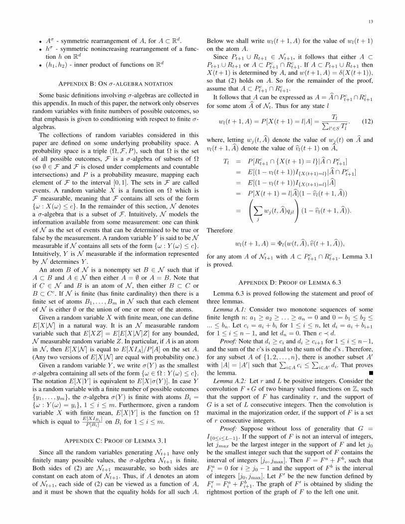
Some basic definitions involving σ-algebras are collected inthis appendix. In much of this paper, the network only observesrandom variables with finite numbers of possible outcomes, sothat emphasis is given to conditioning with respect to finite σ-algebras.

The collections of random variables considered in thispaper are defined on some underlying probability space. Aprobability space is a triple (Ω,F , P ), such that Ω is the setof all possible outcomes, F is a σ-algebra of subsets of Ω(so ∅ ∈ F and F is closed under complements and countableintersections) and P is a probability measure, mapping eachelement of F to the interval [0, 1]. The sets in F are calledevents. A random variable X is a function on Ω which isF measurable, meaning that F contains all sets of the formω : X(ω) ≤ c. In the remainder of this section, N denotesa σ-algebra that is a subset of F . Intuitively, N models theinformation available from some measurement: one can thinkof N as the set of events that can be determined to be true orfalse by the measurement. A random variable Y is said to beNmeasurable if N contains all sets of the form ω : Y (ω) ≤ c.Intuitively, Y is N measurable if the information representedby N determines Y .

An atom B of N is a nonempty set B ∈ N such that ifA ⊂ B and A ∈ N then either A = ∅ or A = B. Note thatif C ∈ N and B is an atom of N , then either B ⊂ C orB ⊂ Cc. If N is finite (has finite cardinality) then there is afinite set of atoms B1, . . . , Bm in N such that each elementof N is either ∅ or the union of one or more of the atoms.

Given a random variable X with finite mean, one can defineE[X|N ] in a natural way. It is an N measurable randomvariable such that E[XZ] = E[E[X|N ]Z] for any bounded,N measurable random variable Z. In particular, if A is an atomin N , then E[X|N ] is equal to E[XIA]/P [A] on the set A.(Any two versions of E[X|N ] are equal with probability one.)

Given a random variable Y , we write σ(Y ) as the smallestσ-algebra containing all sets of the form ω ∈ Ω : Y (ω) ≤ c.The notation E[X|Y ] is equivalent to E[X|σ(Y )]. In case Yis a random variable with a finite number of possible outcomesy1, . . . , ym, the σ-algebra σ(Y ) is finite with atoms Bi =ω : Y (ω) = yi, 1 ≤ i ≤ m. Furthermore, given a randomvariable X with finite mean, E[X|Y ] is the function on Ωwhich is equal to E[XIBi ]

P [Bi]on Bi for 1 ≤ i ≤ m.

APPENDIX C: PROOF OF LEMMA 3.1

Since all the random variables generating Nt+1 have onlyfinitely many possible values, the σ-algebra Nt+1 is finite.Both sides of (2) are Nt+1 measurable, so both sides areconstant on each atom of Nt+1. Thus, if A denotes an atomof Nt+1, each side of (2) can be viewed as a function of A,and it must be shown that the equality holds for all such A.

Below we shall write wl(t+ 1, A) for the value of wl(t+ 1)on the atom A.

Since Pt+1 ∪ Rt+1 ∈ Nt+1, it follows that either A ⊂Pt+1 ∪Rt+1 or A ⊂ P ct+1 ∩Rct+1. If A ⊂ Pt+1 ∪Rt+1 thenX(t+ 1) is determined by A, and w(t+ 1, A) = δ(X(t+ 1)),so that (2) holds on A. So for the remainder of the proof,assume that A ⊂ P ct+1 ∩Rct+1.

It follows that A can be expressed as A = A∩P ct+1∩Rct+1

for some atom A of Nt. Thus for any state l

wl(t+ 1, A) = P [X(t+ 1) = l|A] =Tl∑l′∈S T

′l

. (12)

where, letting wj(t, A) denote the value of wj(t) on A andvl(t+ 1, A) denote the value of vl(t+ 1) on A,

Tl = P [Rct+1 ∩ X(t+ 1) = l|A ∩ P ct+1]

= E[(1− vl(t+ 1))IX(t+1)=l|A ∩ P ct+1]

= E[(1− vl(t+ 1))IX(t+1)=l|A]

= P [X(t+ 1) = l|A](1− vl(t+ 1, A))

=

∑j

wj(t, A)qjl

(1− vl(t+ 1, A)).

Therefore

wl(t+ 1, A) = Φl(w(t, A), v(t+ 1, A)),

for any atom A of Nt+1 with A ⊂ P ct+1 ∩Rct+1. Lemma 3.1is proved.

APPENDIX D: PROOF OF LEMMA 6.3

Lemma 6.3 is proved following the statement and proof ofthree lemmas.

Lemma A.1: Consider two monotone sequences of somefinite length n: a1 ≥ a2 ≥ . . . ≥ an = 0 and 0 = b1 ≤ b2 ≤... ≤ bn. Let ci = ai + bi for 1 ≤ i ≤ n, let di = ai + bi+1

for 1 ≤ i ≤ n− 1, and let dn = 0. Then c ≺ d.Proof: Note that di ≥ ci and di ≥ ci+1 for 1 ≤ i ≤ n−1,

and the sum of the c’s is equal to the sum of the d’s . Therefore,for any subset A of 1, 2, . . . , n, there is another subset A′

with |A| = |A′| such that∑i∈A ci ≤

∑i∈A′ di. That proves

the lemma.Lemma A.2: Let r and L be positive integers. Consider the

convolution F ∗G of two binary valued functions on Z, suchthat the support of F has cardinality r, and the support ofG is a set of L consecutive integers. Then the convolution ismaximal in the majorization order, if the support of F is a setof r consecutive integers.

Proof: Suppose without loss of generality that G =I0≤i≤L−1. If the support of F is not an interval of integers,let jmax be the largest integer in the support of F and let j0be the smallest integer such that the support of F contains theinterval of integers [jo, jmax]. Then F = F a + F b, such thatF ai = 0 for i ≥ j0 − 1 and the support of F b is the intervalof integers [j0, jmax]. Let F ′ be the new function defined byF ′i = F ai + F bi+1. The graph of F ′ is obtained by sliding therightmost portion of the graph of F to the left one unit.

14

We claim that F ∗G ≺ F ′∗G. To see this, note that F ∗G =F a ∗ G + F b ∗ G. The idea of the proof is to focus on theinterval of integers I = [j0−1, j0+r−2] and appeal to LemmaA.1. The function F a ∗G is nonincreasing on I , it takes valuezero at the right endpoint of I , and it is also zero everywhereto the right of I . The function F b ∗G is nondecreasing on I ,it takes value zero at the left endpoint of I , and it is also zeroeverywhere to the left of I . The convolution F ′∗G is the sameas F ∗G except the second function F b ∗G is shifted one unitto the right. Lemma A.1 thus implies that F ∗ G ≺ F ′ ∗ G.This procedure can be repeated until F is reduced to a functionwith support being a set of r consecutive integers. The lemmais proved.

Lemma A.3: Let r ≥ 1 and consider the convolution F ∗ bsuch that F is a binary valued function on the integers withsupport of cardinality r. Then the convolution is maximalin the majorization order if the support of F consists of rconsecutive integers.

Proof: For i ≥ 0, let b(i) denote the uniform probabilitydistribution on the interval [−i, i], of L = 2i+1 integers. Thelemma is true if b = b(i) for some i by Lemma A.2. Let F ∗

denote the unique neat binary valued function with support ofcardinality r. Note that F ∗ ∗ b(i) is neat for all i ≥ 0 becauseboth b(i) and F ∗ are neat. In general, b can be written asb =

∑∞i=0 λib

(i) for some probability distribution λ on Z+.Therefore, for any binary F with support of cardinality r,

b ∗ F =∑i

λi(b(i) ∗ F )(a)≺∑i

λi(b(i) ∗ F )↓

(b)≺

∑i

λi(b(i) ∗ F ∗)↓ = (b ∗ F ∗)↓ ≡ b ∗ F ∗.

Here (a) follows from the fact that taking nondecreasingrearrangements of probability distributions before adding themincreases the sum in the majorization order, and (b) followsfrom Lemma A.2.

Proof of Lemma 6.3 Fix r ≥ 1, let F range over all binaryvalued functions on Z with support of cardinality r, and letF ∗ denote the unique choice of F that is neat. Use “(µ, ν)”to denote inner products.

r∑i=1

(µ ∗ b)[i] = maxF

(µ ∗ b, F ) = maxF

(µ, b ∗ F )

(a)

≤ maxF

(µ↓, (b ∗ F )↓)

(b)

≤ (µ↓, (b ∗ F ∗)↓)

≤ (ν↓, (b ∗ F ∗)↓)(c)= (ν, b ∗ F ∗)

= (ν ∗ b, F ∗) (d)=

r∑i=1

(ν ∗ b)[i]

Here, (a) follows from the fact that rearranging each oftwo distributions in nonincreasing order increases their innerproduct, (b) follows from Lemma A.3 and the monotonicityof µ↓, (c) follows from the fact that both ν and b ∗ F ∗ areneat, so their innner product is the same as the inner productof their rearranged probability distributions, and (d) followsfrom the fact that ν ∗ b is neat.

ACKNOWLEDGMENT

The authors are grateful for useful discussions with Rong-Rong Chen and Richard Sowers.

REFERENCES

[1] I.F. Akyildiz, J.S.M. Ho, and Y.B Lin, “Movement-based location updateand selective paging for PCS networks,” IEEE/ACM Trans. Networking,vol. 4, pp. 629–638, August 1996.

[2] F. Anjum, L. Tassiulas , and M. Shayman ” Optimal paging for mobilelocation tracking ,” Adv. in Performance Analysis , vol. 3. pp. 153-178,March 2002.

[3] A. Bar-Noy and I. Kessler, “Tracking mobile users in wireless commu-nication networks,” Proc. IEEE Infocom, pp. 1232–1239, 1993.

[4] A. Bar-Noy, I. Kessler, and M. Sidi, “Mobile users: To update or notto update?” IEEE/ACM Trans. Networking, vol. 4, pp. 629–638, August1996.

[5] D. P. Bertsekas, Dynamic Programming and Optimal Control, Vol. I.Athena Scientific, Belmont, MA. 1995.

[6] D. P. Bertsekas, Dynamic Programming and Optimal Control, Vol. II.Athena Scientific, Belmont, MA. 1995.

[7] D. P. Bertsekas and J. N. Tsitsiklis, Neuro-Dynamic Programming,Athena Scientific, Belmont, MA. 1996.

[8] C. Cachin, Entropy Measures and Unconditional Security in Cryptogra-phy, PhD thesis, Swiss Federal Institute of Technology Zrich, 1997.

[9] A. De Santis, A.G. Gaggia, and U. Vaccaro, “Bounds on entropy in aguessing game,” IEEE Trans. Information Theory, vol. 47, pp. 468 - 473,2001.

[10] B. Hajek, “Jointly optimal paging and registration for a symmetricrandom walk,” IEEE Information Theory Workshop, Bangalore, India,pp. 20-23, October 2002.

[11] B. Hajek, K. Mitzel, and S. Yang, ”Paging and registration in cellularnetworks: jointly optimal policies and an iterative algorithm,” IEEEINFOCOM 2003, March 30-April 3, pp. 524 - 532, 2003.

[12] B. Krishnamachari, R.-H. Gau, S. B. Wicker, and Z. J. Haas, ”Optimalsequential paging in cellular networks,” ACM Wireless Networks, vol. 10,no. 2, pp. 121-131, March 2004.

[13] E.H. Lieb and M. Loss, Analysis, second edition, American Mathemat-ical Society, Providence, 2001.

[14] S. Madhavapeddy, K. Basu, and A. Roberts, “Adaptive paging algorithmsfor cellular systems,” Proc. 45th IEEE Vehicular Technology Conference,vol. 2, pp. 976–980, 1995.

[15] U. Madhow, M. L. Honig, and K. Steiglitz, “Optimization of wirelessresources for personal communications mobility tracking,” IEEE/ACMTrans. Networking, vol. 3, pp. 698–707, December 1995.

[16] A.W. Marshall and I. Olkin, Inequalities: Theory of Majorization andIts Applications, Academic Press, New York, 1979.

[17] J.L. Massey, “Guessing and entropy,” Prof. 2004 IEEE InternationalSymposium on Information Theory, p. 204, Trondheim, Norway, 1994.

[18] R. Rezaiifar and A. Makowski, ”From optimal search theory to sequen-tial paging in cellular networks”, IEEE J. Selected Areas in Comm, vol.15, no. 7, pp. 1253-1264, September 1997.

[19] F. Riesz, “Sur une inegalite integrale. J. London Mathematical Society,vol. 5, pp. 162-168, 1930.

[20] C. Rose and R. Yates, “Minimizing the average cost of paging underdelay constraints,” Wireless Networks, vol. 1, pp. 211–219, 1995.

[21] C. Rose, “Minimizing the average cost of paging and registration: Atimer-based method,” Wireless Networks, vol. 2, pp. 109–116, 1996.

[22] C. Rose, “State-based paging/registration:a greedy technique,” IEEETrans. on Vehicular Technology, vol. 48, pp. 166–173, January 1999.

[23] W. Wang, I. F. Akyildiz, and G. L. Stuber, “Effective paging schemeswith delay bounds as QoS constraints in wireless systems,” WirelessNetworks, vol. 7, pp. 455–466, 2001.