,

Introduction

HYDRAULICS BRANCH OFFICIAL FILE COPY

PR tDICTION OF DJSSOLVFD GAS AT HYDRAU LI C STRUCTURES

by Perry L. Johns on 1/, A.M. ASCE and Danny L. King 27, M. ASCE

With the incr eased interest in the effects of hydraulic structures on the di sso l ved qas concentration of the flow, it becomes desirable to be ab le to predict how particular structures operating under specific conditions wil l chanqe the dissolved gas concentration.

At existing structures a predictive ab i l i ty wou ld enable the fac ili ty operator to select the method of re lease that would have the mos t desi rable effect on the dissolved qas concentrat ion of the flow. Prototype data ind icate that the chanqe in the dissolved qas concentrat ion is de pendent on the type of structure t hrough which the flow passes, the maqnitude of the discharge, th e barometric pressure, and the water temperature. To estab li sh an operating cr iteria fo r each structure based on ac tual measurement of resu lting di sso l ved gas co ncen­trations wou ld be a difficult task. A predicti ve ability co ul d yield an understandinq of a st ru cture's potential and al low preparat ion for the possible consequences, even if th e structure had ne ver operated.

Al so, wi th a predictive ahility designers wou ld have an addit ional factor which cou ld be con sidered in struct ure selection. Oependinq on the s itu ation, i t is conceivabl e that the dissolverl gas potential might eve n co ntrol the desiqn. Plnnners co uld also use a predictive ab ility to eval uate the potential effects of a s ingl e hydrau l ic structure, or a seri es of hydraulic struct ures, on a r iver.

Initially, the dissolv ed gas concentrat ion above the structure (both oxygen and nitrogen) is equa l to the concentration estab lished by t he i nflow inq st re am. The nit rooen, be i ng re l ati ve ly inert, wil l maintain this conce ntra­ti on for quite some time. The oxyqen, however, especia lly in the lower depths of a resevo ir, may be dep let ed from the decay i ng of organic materia l . Thus , if water is released it may be low in disso l ved oxygen and yet may conceivably be hiqh in dissolved nit ro gen. Furthermore, the water may be high in biochem­ical oxygen demand (BOD ) which wou ld reduce the di ssolved oxygen concentration in the stream below the dam. Theref ore, the analysis sho uld be ab l e to evaluate how effectively structures increase depleted gas concentrati ons as well as evaluate whether supersaturated condi t ions might be created.

Such predict ive methods have been deve loped for the spi ll ways of th e U.S. Army Corps of Enqineers dams on th e Co l umbia River (1). Most of these s tructu res are qeometrica ll y s imil ar. They are low head, run-of-the-river st ructure s, with qate-contro ll ed oqee spillways. The sti lli nq basins are al so of s imilar desiqn . This similarity enabled the development of a predictive ana lysis th at i s qu i te satisfactory for the structures co nside red. The Rureau of Rec lama­tion has few str uctures that correspond to these Co lumbi a Rive r dams. In qeneral, Rureau structures vary widely i n type and size. Thus, a much more generalizerl pred ict i ve ana lysis is required for s iqni f icant application.

J/ Hydraulic Enqinee r, Rureau of Reclamation, Denver, Co lorado ~/ rhief, Hydraul i cs Branch, Burea11 of Reclamati on, Denver, Co lor ado

John son arid King

.. As a basis for development of the analysis, the following data were collected:

1. Reservoir water temperature, dissolved oxygen concentrat ion, and dissolved nitrogen concentration at the elevation from which the water is withdrawn

2. Discharge and a record of which gates or valves are operat i ng if releases are being controlled

3. Tailwater elevation, temperature, and dissolved oxygen and nitrogen concentrations in the tailrace

4 . Loca l barometric pressure 5. Photoaraphs of the structure operatinq and dimensioned drawinqs of the

structure's confiquration

By fa l l of 1973 the monitorinq proqram of the Bureau's Eng i neering and Research Center had reached ln sites and had observed 24 structures in operation. Fo rty-nine different operating cond iti ons had been studied . In addition the Pacific Northwest Reaion of the Bureau of Reclamation has closel y stud ied Grand Coulee Dam and made observatio ns at 36 other sites. The Upper Missouri Reqion of the Bureau has performed monito ring at Yellowtail Afterbay Dam. Combined, these data provided an adequate base from which the predictive analysis could be deve loped.

Analysis

The process of gas transfer is described by the equation :

C(t) = Cs - (Cs - Cr ) e - Kt ( 1)

where C(t) = final dissolved gas concentrati on Cs = saturation concentration Cr = initial concentration K = a constant of proportionality t = time

C(t), Cs, and Cr are co ncentrations in mq/L of water.

Equation 1 shows that the final dissolved gas concent ration, C(t), below a hydraulic structure is dependent on the init i al concentration, Cr, in the reservoir, the saturation concentration, Cs, in the sti lling basin, the lenath of ti me, t, that qas is be inq di sso lved into the flow, and a constant, K, that would be expected to vary with the spec ifi c hydraulic structure and ooeratina cond iti on. Cl will be either set at a known level or assumed. The other three parameters (Cs, t, and K) are depende nt on th e type of stucture, operatinq condition, temperature, and baromet ric pressure. Efforts were directed at evaluatina Cs, t, and K computationally.

The saturation co ncent r at ion level, Cs, in the st illing bas in, is dependent on the pressure th at can be developed in the basin and the water temperature. The pressure obtained in a stilling basin i s dependent on the depth of water over the flow in which the bubbles are entrained and the barometric pressure. Thus, surface water at sea level will ho ld 33 percent more gas than surface water at an elevat ion of 8000 ft (?438 m) . Also, water at the surface of a pool will hold 50 percent less qas than water at a depth of 34 ft (10.4 m). Barometric pressure is basically contro ll ed by the elevation at which the

2 Johnson and King

... ~ ~.

..

structure is located, with dai l y fluctuations that result from atmospheric conditions. The effects caused by daily fluctuat ions in atmospher ic pressure are not large but they may be significant and should be cons idered in the evaluation of Cs. In this analysis measured barometric pressures were used when available. If measured va l ues were not avai l able a standard atmos­phere was assumed and barometric pressures were computed according to e l evation.

The depth of water over the flow in which gas is being dissolved is generally dependent on the depth of water in the stilling basin. Thus, variations in the tailwater elevation wi ll have some effect. Throughout this analysis a water depth equal to two-thirds of the basin depth was used to compute satura­tion concentrations. It was thought that in i tially the fair ly compact jet from a spillway or outlet would penetrate to the f loor of the stilling basin. The flow would then be deflected downstream and out of the basin. As the flow moved through the basin it would be diffused and its velocity reduced . This diffusion would be linear and result in a triangular pattern with the average depth through the diffusion being two-thirds of the total basin depth. Bubbles r ising from the flow and incomplete flow penetration wou ld tend to reduce this average depth, but the two-thirds depth was considered representa­tive and therefore used in the ana lysis. A major point of support for the two-thirds depth assumption is the fact that later applications proved the assumption reasonable. If the flow being stud ied does not penetrate to the bottom of the pool the maximum depth of flow penetration may be used in this calculation in place of the basin dept h.

Evaluation of Cs is achieved by summing the barometric pressure and two-th i rds of the basin depth (expressed in mm of Hg ) and dividing this total pressure by standard atmosp heric pressure (760 mm of Hg) to obtain the average absolute pressure on the dissolving bubbles in terms of atmospheres. This average absolute pressure is then multiplied by the dissolved gas sat ur ation concentra­tion at sea leve l, for the desired water temperature, to obtain Cs.

The next parameter from equation 1 to be considered is the time, t. It i s representative of the length of time that the inflowing jet with entra i ned air is under pressure in the stilling basin and, thus, the length of time that gas is being dissolved in the flow. Consideration of time revealed two possib l e limitations that could control its value. First, it wou ld seem that given sufficient time the entrained air bubbles would rise out of the flow and end the disso lving of gas. In some cases it would seem that an evaluation of this bubble rise time could be used to represent time. On the other hand, s itua­tions mig ht occur where the fl ow wit.h entra ined air would pass through the basin and be deflected to a sha ll ow depth in a fairly short time. Therefore , the actua l length of time required for the flow to pass through the basin could represent t. During this analysis the assumpt ion was made that ei ther of these time periods might be critica l in specific situations. For each f l ow condition and structure studied, twas evaluated for both limitations. The smaller of the two computed values was considered applicable to the particular situ ation and was used i n the remainder of the analysis.

Bubble rise time. - Eval uation oft based on the bubble rise time, t1, would be, if strictly pursued, a very complex computation which would probab ly produce questionable results. Th e vertical dimension of the jet (th ickness of jet that the bubble would rise through) is never constant. The time, t, based on bubble ri se time, t1, was evaluated by dividing the calculated vert i cal

3 Johnson and Ki ng

.. •.

th ick ness of the jet at the ta il water surface hy the terminal rise ve locity of the bubb le. By trial and er ror, it was rletermin erl that an assumed o.n 2R-inch (0.7-mm) diameter buhble with a theoretical termin al ve locity of 0. 696 ft/s (0. 2 m/s) yielded the most consistent results with respect to observed prototype conditions. Al so, when an analys is was developed that predicted K (equation 1) from two dimensionless parameters, i t was found that the 0.02R-inch-d i ameter buhble yielded pred icted values of K that were consistent with the predicted values of K based on the basin retention time.

Basin retention time. - Computation of the fl ow retention time , t2, in the bas i n is accomplished by dividinq the path lenqth of the flow by the averaqe f low veloc ity alonq the pat h. The path lenath is qenera lly controlled by the basin shape. The path lengt h is the dis tance from the po int at which the jet enters the tai l water pool to the point at which the ma jority of the flow is directed t oward the surface and, therefore, into a lower pressure zone. If a large portion of the flow is deflec ted upward at a point by baffl e piers, for examp le, this point would be considered the end of the path.

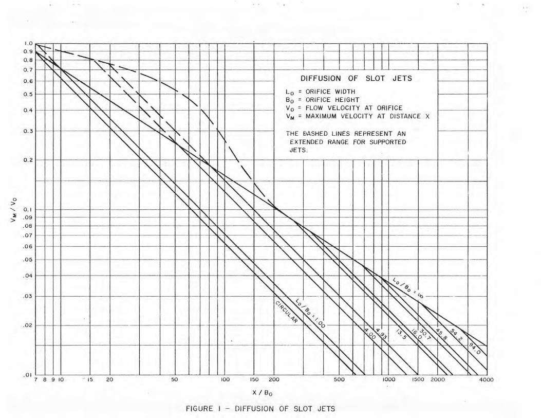
To compute t he averaqe flow vel ocity over the path lena th, the first step is to obtain the jet ve locity at the tailwater surface (or at t he start of the flow path) from t he prev ious ana lysis of bubble rise time. To determine the averaqe flow velocity, the velocity at the end of the path must be found. Th is is done thro uqh the use of fiqure 1 which is a summary of information from studies of jet diffusion by Yevdjevich (2) and Henry (3). Observation of velocity distribut ions in jet diffusions indic ates that half of the maximum ve locity would be an approximation of the jet's averaqe velocity at the end of the f low path. This averaae velocity miqht al so be evaluated by dividi ng the discharae, 0, by the channel cross sect ional area, A, whi ch would assume complete diffusion of the jet. The larqer of the computed vel oc i ties shou ld be used, since the averaqe jet velocity at the end of the path could be hiqher, bu t not lower than the averaae velocity through the full cross section. The velocities at th e beqinninq and end of the flow path are then averaged, the n this averaqe is divided into the flow path lenath to obtain the basin flow re tent ion time (t2 ). As previously stated, the value oft to be used in equat ion 1 is the sma ller of the two computed values (t1 or t 2).

The f in al term in equation 1 to be eva l uated is K. K is unlike the other terms eva l uat ed in that it is not direct ly representative of any specific physical parameter. K is a measure of the abi lity of a particular structure, operating under a particular conditi on , to dissolve gas. It is rep resen t ati ve of the deqree of air entrai nment and the rate at which the water at the gas-liquid in terface is rep leni shed .

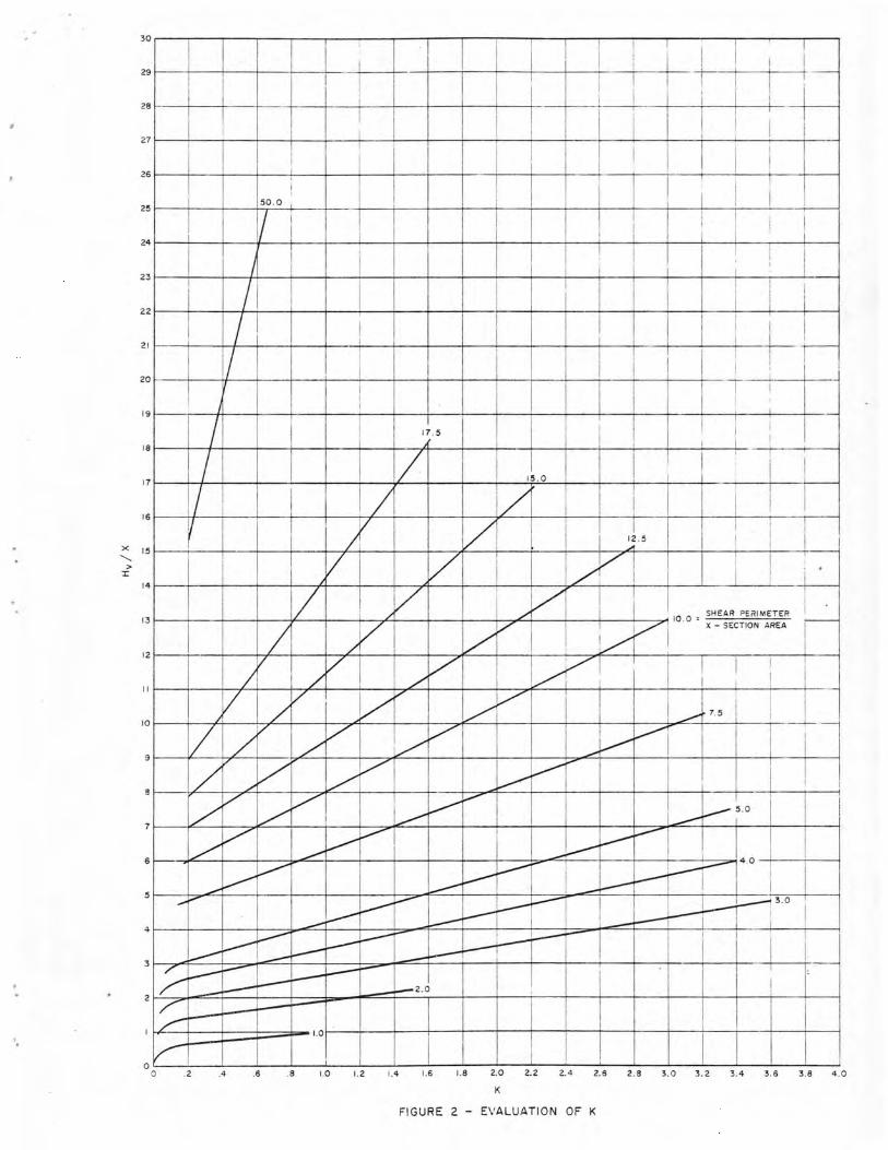
It appears that K is dependent on ly on t he hyd raulic performance of th e basin. Attempts to find a predi ctive proced ure t hat could be used to evaluate K resulted in the curves shown in fiqure 2. To obta in these curves the prototype data were manipulated in to . various parameters unt il us eable resu lts were fou nd . On ly dissolved nitroqen data were us ed in the deve lopment due to the stabil i ty of nitroqen. At a few of the reservoirs data wer e col lected at severa l depths. Th ese data indicated th at dissolved oxygen concentrations may vary wi del y throuqh the depth of a reservoir but that dissolved nitroge n concentrations are fa ir ly const ant. At some ot her reservoirs dis solved qas data were co llected only near the surface and no t at the withdrawal elevation. Therefore, if dis solved nitroqen and oxyqen concentrat ions are measu red at t he

4 Johnson and King

. , ..

reservoir surface and the withdrawa l s are made from deep in the reservoir, the measured values of the initial di ssolved gas concentrati ons, C1, are probably more accurate for nitrogen than oxygen. Even though dissolved nitrogen data were used as a base for the analysis, app li cation of the ana lysis for observed prototype conditions indicates that resulting disso lved oxygen levels may also be predicted.

Fiqure 2 shows that the value of K is dependen t on two parameters. The first is Hv/X, the velocity head, Hv, at the tailwater surface divided by the flow path length X. Hv/X is an energy gradient parameter for the flow; it relates the amount of energy in the flow to the path length in the bas in over which the energy is dissipated. The greater the value of Hv/X the more turbu lent the basin flow and the larger the resulting K value. The path length used corresponds to the va lue oft selected . If tz is applicable, then the value used for X would be the path length used to evaluate tz. But if t1 is applicable, t he path length is adjusted to determine the effective path lenqth for the time interval, that is , the length of time the bubbl es remain in the jet. Flow decelerat ion is assumed linear and t he ratio of t1/t2 is multiplied by the tota l velocity drop to determine the ve locity drop along the adjusted path length. The average ve loc i ty along the adjusted path is the n computed (initial ve loc i ty minus one-half the velocity drop) and multiplied by t1 to determ ine the adjusted path length .

The other parameter on which the value of K is based is a ratio of the shear perimeter of the jet to the jet's cross-sectiona l area at the ta il water surf ace. This term is a measure of the jet compactness and shape. The shear perimeter for a jet is defined as the length of the jet's perimeter over which a shearing action is occurring between the jet and t he water of the st i l l ing basin pool. For a free jet plunging into a poo l the shear perimeter would equal the total perimeter of the jet, while for a flow passing down a chute spillway and into a bas in the shear perimeter would be the chute width at the tailwater surface. Situations exist where the walls of the stil li ng basin are offset from the jet entering the basin. If th i s off set is sma ll , questions may arise as to whether the sides of the jet should be included in the shear perimeter. This is a judgment factor and is probab ly best handled by i ndivid­ual consideration. Another common struct ure that might raise a similar question would be a hollow jet val ve discharging into a pool. Although the flow wou ld have a ring-shaped cross-section, on ly the outside perimeter should be included in t he evaluat ion. In general, if it appears that sign ifi-cant shear will occur along the section of perimeter in question then those lengths should be inc luded in the analysis.

With the evaluation of K from fiqure 2, equation 1 may be applied and the final dissolved gas concentration, C(t), determined. The proto t ype data were used extensively to eva luate the coefficients that are applied throughout the analysis. This empirical approach is mandatory because of the complexity of the flows being considered. Very few of t he situat ions studi ed have clear ly defined flow conditions that are well suited for direct analys is. Not on ly are the jets that le ave the spillway chutes, the va lves, and the gates often quite comp lex, but the sti lli nq basi n pools are equally complex. Any ana lys is of these flow conditions wou ld be quite invo lved and the accuracy wou ld be questionable. However, the coefficients resulting from this ana lysis do have a rational basis and are representative of the various physica l parameters. The coeff ici ents can be interpreted to yie ld addit ional insight into the siqn ifi canc e of the various factors.

5 Jo hnson and King

Althouoh some entrainment of air is needed for the dissolved qas uptake to occur, the amount of entrained air required seems to be quite small. At some of the prototype structures releases were exposed only briefly to the air. In some of these cases the water surfaces of the releases were also relative ly smooth. Thus, it is assumed that little air was entrained. This assumption was verified by the small quantities of air that were observed returning to the tailwater surface. However, in some instances, the structures with little apparent air entrainment were amonq the worst in creatinq supersaturated conditions.

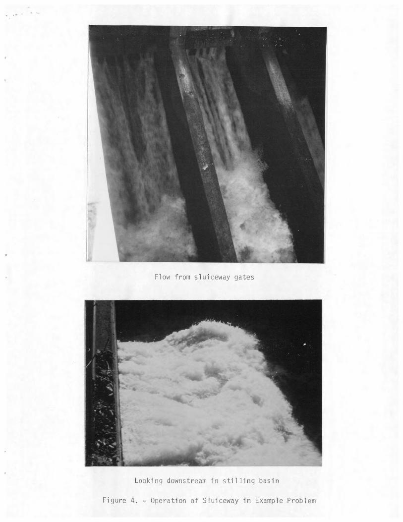
Example Application

Included with the example is a drawinq of the structure (fiqure 3) and photo­graphs (fiqure 4) of operation. The computat ions are described step by step. All crit ical points and all judqments or approximations are discussed and the results of the analysis are compared to actua l field findings. Results are also included for examples for which the ca lcu lations are not shown. Varia­tion s between the observed and ca lcul ated dissolved gas concentrations may be attrihuted to several factors. First, and probably one of the most important, is that the entire analysis was hased on averaqe prototype data. Therefore, some structures wi ll fit t he analysis better than others and some structures will yield more accurate predicted re su lts. A second siqnificant source of variation wou ld be errors in measurina the prototype dissolved gas concentra­tions. The chemical analyses used are not completely accurate, but even more important, samples may be collected from reaions that are not representative of the total flow. Extreme errors of this sort may or may not be obvious . In several cases, two or more readinqs were ava ilable which qave some additional assurance. Variations due to errors in data collect ion may be small or they may be quite larqe. Application of the analysis and use of the graphs may also result in some error, but this error should be small. All factors considered, the resu lts are very encouraqinq.

Example . - Sluiceway. - The fol lowinq information is known:

Reservoir water surface elevation= 3196 ft (974 m) Tailwater surface elevation= 3168 ft (966 m) Baromet ric pressure= 67 7 mm Hg Water temperature= d.4 ·c Discharge= 3550 ft3/s (100 m3/s) Reservoir dissolved nitroaen concentrat ion= 104 percent of saturation RPservo ir disso lved oxyoen concentration= 85 percent

The structural dimensions in fiqure 3 and the photoqraph in figure 4 are also available. From these sources the followinq terms are deduced:

Hv = 3196 - 3168 = 28 ft (8.5 m) Anq le of jet penetration~ 25 ° Ras in depth= 3168 - 3146 = 22 f t (6.7 m) Basin flow pat h lenqth, X ~ 95 ft (29 m)

It should be observed that no head loss was included in the evaluation of the jet velocity head, Hv. For this particular structure, this assumption should he reasonably valid in that the flow path between the control gate and

6 Johnson and King

the still ing basin pool is short and unobstructed. Because of the changing s lo pe of t he flow surface as it enters the st illing bas in , the angl e of penetration was approximated to be 25° below hori zontal . The basin dept h of 22 ft (6. 7 m) was computed for the deepest portion of the pool . Finally, the fl ow path length, X, of 95 ft (29 m) is approxi mately the distance from the point where the jet wou l d attain signifi cant penetration to the end sill of the basin. It was reasoned th at at the end si ll a large portion of the flow wi ll be def lected upward, the flow will no longe r be under the higher pressure, and disso l ving of gases in the basin will be complete. These approximatio ns are quite rough , but attempts to refin e the eva luations would yield only s li ght impro vements and would ca ll for and indicate unwarranted accuracy .

The abso l ute dissolved nit rogen concentrati on in the rese rvoi r is evaluated as the f irst step in the analysis. Thi s is accomplished by referring to appropri­ate standard tables and obtaining the nitrogen sat uration concentration for the specif ic water temperature (4.4 °C) and multiplyi ng i t by the re lative reservoir disso lved nitrogen concentrat i on (104 percent ).

Cr= (1.04) (20.7) = 21.5 mg/L

Next the potentia l abso lute dissolved nitrogen concentration for the stilling basin is computed. As stated before, it is depe ndent on the barometric pressure, water temperature, and bas in depth. Two-thirds of the bas in depth is assumed as the average depth over the flow whi le the gas is being dis solved. Using this approx imati on an average pres sure on the flow (in atmospheres) is computed and multiplied by the abso lu te dissolved nitrogen concentration obtained earl ier.

Cs= 677 + 2/3(22)(~~6.8/13.55) (20 _7) = 27 .4 mg/L

This term has been adjusted to ref lect the barometr ic press ure and, thu s, the structure's elevation. If the barometric pressure is un known, a standard atmosphere may be used.

Two of the term s (Cs and Cr) of equation 1:

C(t) = Cs - (Cs - Cr) e -Kt

have now been evaluated. Th e time, t, that gas is being dissolved, is the next term of interest. The bubble r ise ti me, t1, i s evaluated first. To do this, the vertical dimension of the j et at the ta ilwater surface is fo und . The 28-foot velocity head yields a ve locity of 42.5 ft/s (13 .0 m/s). Th e discharge is then divided by the velocity to obt ain a total flow cross sectional area for t hree gates .

3550/42 .5 = 83.5 ft2 (7 .8 m2)

Assumin~ equa l f l ow through each results in a flow cross sectiona l area of 27 .8 ft (2 .6 m2) for a s ingle gate When eq ual flow conditions are assumed for the gates, the ana lysis of each individu al gate is identica l and, thus, the analysis of the flow for only one gate will pr edict th e performance of the entire structure. If the flow cross section al area is then divided by t he qate width ( 8 ft) the flow depth is determ in ed .

27.8/8 = 3.5 ft (1 .1 m)

7 Johnson and King

Since the flow is no t ho r izontal the fl ow depth must be divided by the cosine of the anqle of penetrat ion to obta i n the vertical dimens i on of the jet.

3.5/cos 25° = 3.5/0.9063 = 3.9 ft (1.2 m)

If this distance is then divided by the terminal bubb l e veloc ity, a bub ble rise time, t, i s obtained.

t 1 = 3.9/0.696 = 5.6 seconds

The lenqth of ti me, that the f l ow is at f igure 1 are used. dept h, R0 •

t, is al so evaluated by cons idering the l ength of t ime an effective depth in the bas i n. To do th i s t he cur ves i n First, the flow path length, X, i s divided by the fl ow

X/B 0 = 95/3.5 = 27 .1

The flow width (L 0 ) is then divided by the f low depth.

L0 /B 0 = 8/3.5 = 2.3

Fiaure 1 is then referred to and the rat io of the maximum ve locity , Vm, wi thin the velocity distribution at the end of the flow path to the in i tia l flow velocity, V0 , is obtained.

or

Vm = (0 .36)(42.5) = 15.3 ft/s (4.7 m/s)

If the averaae flow velocity at the end of the path is then assumed to be one-half of Vm, an averaqe velocity through the basin can be determined .

V = ((15.3)/2 + 42.5)/2 = 25.l ft/s (7 .7 m/s)

An averaqe ve locity at the end of the path based on cross sect ional area and discharae would be:

3550/((22)(28)) = 5.8 ft/s (1.8 m/s)

Thi s is less than (15.3/2) or 7.7 ft/s (2.3 m/s), so 7.7 ft/s should be used.

The path lenqth divided by this averaqe velocity qi ves the basi n retent ion t ime~

tz = 95/25 . l = 3.8 seconds

The smaller of the two comouted times is the one that is app li cabl e to the probl em . For this particular case, the shorter time is 3.8 seconds, the t ime interva l based on the f l ow ve locity .

The final term to be evaluated is K, which is fo und thro ugh t he use of f igure 2. To apply fiqurr ?, two parametPrs must he computed . Th e rat io of the ve loc ity

R John son and Ki ng

head, Hv, to the appropriate flow path lenqth, X, is Hv/X. If the time interval used i s based on basin retention time, the basin flow path lengt h (evaluated from the basin geometry) is used. If the sma l ler time results from the consideration of the bubble rise t ime then the flow path length to be us ed is less then the basin flow path l ength. For the sam ple problem the time based on the basin retention time is the smal ler so the initially determined path lenqth of 95 ft (29 m) is used. Therefore,

Hv/X = 28/95 = 0.295

For application of fiqure 2, the second parameter that must be evaluated is the ratio of the shear perimeter length of the jet to the cross sectio na l area of the jet . For this problem the shear perimeter is the jet width plus the jet height for each side or

8 + 3.5 + 3.5 = 15.0 ft (4.n m)

The cross sectional area has already been found to be 27.8 ft2 (2.6 m2). Thus the ratio is

15.0/27.8 = 0.54

The value of K is 0.1 from fiqure 2. The user will note the possibility of interpolation error. All the terms may no~ be substituted into equation 1 and a dissolved nitrogen concentration that is not corrected for barome tric pressure is obtained.

C(t) = 27.4 - (27.4 - 21.S) e-(0 .1)(3 .8) = 23.4 mg/L

If this is then divided by the saturat ion concentration, the percent nitrogen saturation is obtained.

23.4/20.7 x 100 = 113 pe rcent

The observed value for nitrogen, N2 was also 113 percent . To obtain a predicted absolute concentration, multiply the predicted percentage by the absolute concentration ad justed for barometric pressure.

(l .13)(677/760)(20 .7) = 20.8 m~/L of N2

Considerinq dissolved oxyqen, we compute:

Cr = (0.85)(12 .9) = 11.0 mq/L

where 12.9 mg/L is the saturation concentration of oxygen at 4.4 ·c.

Also:

Cs - 677 + 2/3(22)(304.8/13.55) ( , = 12.9)

t = 3.8 seconds

K = 0.1

g

17 .1 mg/L

Johnson and King

all of which foll ow from the ni troaen calculati ons ahove. Applyinq equa­t ion 1:

C(t ) = 17 .1 - (1 7.1 - Jl .0) e -(0 .1 )(3 .8) = 12.9 mg/L

Th e percent oxyaen saturation ca l cu lated is:

12.9/12 .9 x 100 = 100 percent

The actual observed value f or oxygen, Oz was also 100 pe rcent.

An approx imat ion of the percent total dissolved gas would be:

(100) (23.4 + 12.0)/(20.7 + 12 .9) = 105 percent

Thi s cons iders nitroge n and oxyaen, which toget her compr ise over 99 percent of the total dissolved gas .

Several other examp les were ca l cu l ated with the following resu lts:

Ca l cu lated Observed St ructure N2 02 N2 02

Sp ill way with ro 11 er bucket, 201% 197% 199'.Yo 1/ 2/ t hree qates operatin g

Chute sp illway into hydrau li c 116 112 116 108 jump bas in

Au xi liary out let wor ks (four dis- 148 145 147 130 4/ charqes) t hro uq h spillway 153 15 2 155 132 4/ face into hydraulic jump basin 15 3 153 158 134 4/

154 153 125 ]_/ 130 4/

Chute spi llway with fli p bucket 109 2/ 103 2/ an d shallow plunge pool

1/ Considerab ly less af t er dilut ion by powerp l an t di scharge. 2/ Data not ava il able. 3/ Bel i eve that gas escaped from samp le. 4/ Possib ly lower because of heavy oraani c load i ng.

Conclusions

1. Given the ve locity head of the inflow jet at the t ailwate r surface, the anale of pe netratio n of the j et into the t ailwater , the shape of th e jet, the bas i n lenath and dep th, the water temperature, t he baromet ri c pressure, and the i nitia l dissolved qas levels in t he reservoir, the dissolved gas levels that will resu lt from the passaae of flow thro uqh a hydrau li c st ructure can be predicted wit h r easonable accuracy. Model stud i es can be used to great ad vantaae in rlefinina the hydraul i c characterist ics to be used in t he ana lysis .

10 Johnson and King

2. Th e basic equation developed to predict the resulting dissolved gas concentrations i s:

C(t) = Cs - (Cs - Cr) e -Kt

where C(t) is the dissolved gas concentration created by the hydr aulic struc­ture , C1 is the disso lved gas concentration in the reservoir, Cs is the saturated disso lved gas concentration at a depth which is two - thi rds of the maximum basin depth , t is representati ve of the length of t ime during which gas i s being di ssol ved, and K is a constant that varies with structure an d operating condition. A method is developed for prediction of the K value.

11 Johnson and King

APPENDIX - REFERENCES

l. Roesner, L. A., Norton, W. R., "A Nitrogen Gas (N2) Mode l for the Lower Columbia River," Final Report, Water Resources Engineers, Inc ., January 1971

2. Yevdjevich, V. M., "Diff usion of Slot Jets with Finite Orifice Leng t h -Width Ratios," Colorado State University Hydraulics Paper No. 2, December 1965

3. Henry, H. R., Discussion of "Diffusion of Submerged Jets," Paper No. 2409, pp. 687-694, Transactions of the American Society of Civil Engineers, Vol. 115, 1950

12 Johnson and King

Figure 1 - Diffusion of slot jets

Figure 2 - Evaluation of K

Figure 3 Sluiceway in examp le problem

Fi gure 4 - Operat i on of sluiceway in example problem

13 Johnson and King

PREDICTION OF DISSOLVED GAS AT HYDRAULIC STRUCTURES

KEY WORDS: Aeration, Oxygenation, Research, Water quality, Hydrau l ics

ABSTRACT: Hydraulic structures such as stilling basins present an opportunity for oxygenation of oxygen-deficient releases from reservoirs while at the same time posing a potential threat of supersaturation of dissolved gas. This paper presents a proposed method of analysis leading to prediction of the increase or decrease of dissolved gas passing through a hydraulic structure. An equation is presented with coefficients evaluated by analysis of prototype data.

14 Johnson and King

CIVIL ENGINEERING ABSTRACT : A method for predict i ng changes in dissolved gas in water passing through hydraul i c structures is presented . The method was developed by analysis of data from prototype structures .

15 Johnson and King

0 >

" :E >

1.0

0 .9

0 . 8

0.7

0 . 6

0.5

0 . 4

0 . 3

0.2

0 . 1

.09

.08

.07

.06

.05

. 04

.03

.02

. 01

~ i- -

~ ~ -- --' ~ ' ~ ~ ....;._

' ~ ' ' ~

' '- '- ............... "~ ' " " '- '

"' ~" """ " " '- '-

~ ~" " ' ~' ~ ~ ~

~

7 8 9 10 . 15 20

! I

-DIFFUSION OF SLOT JETS

"""' .. = ORIFICE WIDTH Lo

' Bo = ORIFICE HEIGHT

' Vo = FLOW VELOCITY AT ORIFICE

' '\ VM = MAXIMUM VELOCITY AT DISTANCE X

'"\ \.

~ " \ THE E>ASHED LINES REPRESENT AN

~ ~ EXTENDED RANGE FOR SUPPORTED

~ \ JETS .

"' ~ '

~ " ~ ~ l"-. \ ' '\ ~

'r"\

~ ~. ~ "' " ' " "-

' ' ', " "-.

" r"\ ""' f\.. '~ I'\ l"\. "' f\.."' ~ t',..._

"'"' "'"' "~ " ···· ··--

~ ~ "' ~ "' ~ ~ ~~ ~ "' ' ~

~ --,~ (.0

~ ~ ~ ' ~/~ '- 0 "

C}~~ - "' ~ "~~ % ---

~~~ 0~ ~ ~ ' ~~ -~~ ~

"' ..,., "51'

/~~s~ ~~-~ S O ·> ~ " s?

~ . ' ' ~ ~

' ~~~ '

~ ~ 50 100 150 200 500 IOOO 1500 2000 4000

XI Bo

FIGURE I - DIFFUSION OF SLOT JETS

30 ,------,.-I -.------.---.------.--.----1-....,.......___,.---,------,.-....,.......___,.--.-!--.-\--.-1-----..-!\ --.------,-I ________,

I I I I I i \ I I 29

f-----11--+l--_,_I _J_i __ ...... 11 -1-----+---i---+-----+i --+-j--! -+-, - i-: --+!--+-I - 1--:1 ---+-i -28 t----+--- t-----+------i.-----+---+--+----+--+----+--+-

27 1------+-I _____,l~ -+-------+---+-----+:--+-----+------+-------r-~ 1--li -------+------,1~-+-i ----+~-+-! ----+'~+-I ---+-1-----l I ! I : I I I I i

26 t-----+----t-----+---,---+---+--+----+--+----+l- -+---+--+!--+----.---;-----+-1, --+-i --+----1

I 5o .o ; i I ! 25 f-----+--f----+-,,--+---+---4- -+----+--+----+--+---+--+-----+--+----+--,----'---r----1

I / 1 1 : i ; !

::~~~~I ~~~~~~~~~!~~~~~~i~~~~~~~~~~~~~~~1~~~!~~~i~~~1~~~1 ~~~~~~: ~~~! ~~~i ~~ I /I ! I I I I I I

22 !-----+---f--+--+---+....----+---+--+----+--+---+--+---+--+-----+--t----+--;-I--+-----+-----!

21 t----l---+-+-;_1---+-----+------,t-1 __ --i-____ --+----+---·-+---__...l---+-1 _ 1 _L I / i I I I I : ! I

20f-----+---ff----+---+.-----1l---+---+--+---+--+---+--+---l--+-----+--i-- I I I I ! I I

19 1-----;-++--->------+-------<e-------------1--+----,--+-----.--+----+1--+----+--+----+-I --+-----+------<

I. I I ! I i

11 . 5 I i0 f-----+---+--f-----+---+f----+---+---+-----+1---+---+---+----+--+'--+1--+-----'-1- -+--I - ' ----

/ i / 15 . 0 I I I I

I ! 17 f-----+--l--f-----+--------+-_,,,_--+--+----+--'-r-'-"--+--+-----+--+----+-----+--+----1

I/ / / I i 16 --14-, -f-----+---+---+---+/-+----+---+--+v--4,,«---+--+-----+--+l--+-----+-+1-~, --+1-----l

1

/ 1

~ -5 I ! I I I

X 15f-----+--l-----+---+---+--+-4---+---+-----+--+---+--+------ -+-----+--+-----+- -,-~

'i Iv / 1 / ./ I I ! i · 14

t----+--t----+---+l-/---+1,-..----t----t/v----+--+i-./-+~----- 1--+----+-IO.-O ~. -SH-EA~R -PE"-IM~ET-ER--+i -----1

13 / // // I vr! x-SECTIONAREA I

12 1---...--+---+-,,v-+----+-v-,.c....+-1 --/~-+----+--~----1--+1--+~1~ ,- ,----+~ I/./ / , 111

II t------t--r-+-+---+t--7'"--+---t----+-,,,---t--+---t-7"f'----t--+-----+--+------r--t-----+- -r-·-

10 f-----+----A/vf-----f--,~~,-~----,f---,~~/~-jV--!---"71v,c__-f/--t-----+- -t---f-~e::..---+--7. _5 -+i--+l--+--/ /v /v v/ J__..,,.,-~I I

9 f-----+'---'rr---+-- 1r--+-----,-~----,--+-----+- -+-----+~ ::+-----+- -+--+- -+----+--+------j

8 ~i,,L-/--+v----7""'-+//-+----"7"1"'V--,-/--+------+-------+---::...-i:--L..------1__..,,.,----+,.....-+-+-----+---+----+----+--il _1,....----i V _/ ,_..,,...... I I I

71-----¥/-+--~/-i-'-i-! -1----::~----~f-..------il----+-----,~-+-----,--+---:;;;,,oT----==-+~--+5-.0--t- -+----, V I __ .........-- I ---~

6 / _..........-- ~t-- I

~ I ---~ : ---,--- 4.0 -+-,I - I;----; ...... l---'" --- I ---~ I I 5 1---+:.~ +---+--+---+--+---+--::;;;,-"'"F--+-----,,----+----::::;:a-e:::::i----+--+----+--+--+-:;--::,--t----,

......... ___ ..-- I __:.----- I, I _L--+---13.0 1 I

__.L.-- ---1 I --~---i- i i , 41---+--+---+---::::~::...+-- +-----b-F---+-----,--t----J:=-t-=---t--t-----+--+---t--+----,

3 ---v-~--~-- --~.--t----- I i _ i I,·-, ---- ~- +-+ ~ ~-- I,

2 "/7t:_xi---==t===t::;::;::;;;r-r~r-::....:2:.:..:·011111'111- ,--t- 1r- r-r1 ,-- I r/::t=t=====F==i" 1.o~--+---+---+---+--t-----+-1----:-------i------l

0 L----'--'------'--'----'---' ---'--'--'---'----------'-~--'----'----'---'---.J.---'---.J.---J 0 .2 .4 .6 .8 1.0 1. 2 1. 4 1.6 1. 8 2.0 2.2 2.4 2. 6 2.8 3.0 3. 2 3.4 3.6 3.8 4 .0

K

FIGURE 2 - EVALUAT ION OF K

\ I

\ \ \

\ \

\ \

\ \ "' \ \ \_ \

~

El. 31 97 50 ·,

E l. :>19( ,

~ .:,:=·

El.3197.50

/

PLAN

El. 3204.60

I

TO CANAL

/

I I I

I I \

HEAOWORKS

\

\ \ \ \ I

~

~ El. 3172.00

f-~~~IDE GATE~'>----'-------, - [ E l. 3168,00

E l. 3139.00

, . . o · () . • ·- .. 0 : • . • , :

SECTION THRU SLUICEWAY

El , 3204.80

,--.,-,--'----,_ 30°X 13.5' RADIAL GATE

..f_EI. 3172 .00

. ·. · - o . a . E l. 3146.00 o .

0

<> " . . · • ." ."O ·." . _. _

2 0 10 0 20 40 SECTION THRU OVERFLOW WEIR

SCALE I N FEET

FIGURE 3 - SLUICEWAY IN EXAMPLE PROBLEM

. . ~

Fl ow from slui ceway gates

Look in g downstream in s tilling basin

Figure 4. - Operat ion of Sluiceway in Example Problem