Groundwater Hydraulics EHG 315 Dr. Tariq Hassan Bayumi · Groundwater Hydraulics Introduction Groundwater hydraulics is a branch of the hydrogeological sciences that combines groundwater

Dr. Tariq Bayumi EHG315

هيدروليكيا المياه الجوفية315ض جم

Groundwater Hydraulics EHG 315

Dr. Tariq Hassan Bayumi


Groundwater Hydraulics

References

A- English References 1- Kruseman G.P.& DeRidder, N. A., 1990. Analysis and Evaluation of Pumping Test Data. International Institute for Land Reclamation and Improvement, Wageningen, The Netherlands. 2-Sen, Z., 1995. Applied Hydrogeology for Scientists and Engineers. Lewis Publications, Boca Raton. 3-Todd, D. K., 2005 Groundwater Hydrology. John Wiley & Sons. New York. 4- Raghunath, H. M.,1982. Groundwater. Wiley Eastern Ltd., New Delhi.

B- Arabic References:

األردن. -م. هيدروجيولوجية المياه الجوفية. دار البشير، عمان1987خليفة درادكة، -5

السعودية. -هـ. المياه الجوفية. الرياض1422عبدالعزيز البسام، -6

C- Related internet websites: 1- http://www.ngwa.org 2- http://www.lifewater.ca/ndexdril.htm


Contents

Introduction.

Basic concepts and definitions.

Steady radial flow –confined aquifers

Steady radial flow- unconfined aquifers

Relation between discharge and drawdown in steady state flow Unsteady radial flow in confined aquifers (Theis method) Pumping tests- technique and instrumentation

Jacob methods of solution Slope-match method

Large diameter wells- Papadopulos-Cooper method and volumetric method.

Unsteady radial flow in an unconfined aquifers

Unsteady radial flow in an leaky aquifers

Partially penetrating wells Recovery test

Multiple well systems and interference

Well flow near hydrogeological boundaries

Course Grading Course requests and means of evaluation:

1- 2 periodical exams- 20 degrees each 2- Weakly homework, activity and attendance 20 degrees. 3- Final exam – theoretical and practical- 40 degrees.


Groundwater Hydraulics

Introduction

Groundwater hydraulics is a branch of the hydrogeological sciences

that combines groundwater and geology in a quantitative manner. It is mainly concerned with estimating various quantities related to groundwater storage and movement within geological formations. Emphasis is made on aquifer constants, such as hydraulic conductivity, transmissivity, specific yield and storage coefficient in addition to groundwater flow, discharge, drawdown and storage.

This course benefits from other courses such as "Groundwater Geology" and "Elements of Flow through Porous Media". It is a prerequisite for advanced courses like "Well Technology” and Groundwater Modeling".


Basic Concepts and Definitions I- Physical Properties of Aquifers

الخواص الفيزيائية للتكاوين المائية

1- Porosity (η): The porosity of a rock is its property of containing pores or voids. It is defined as the ratio of volume of voids Vv to total volume of medium (rock) VT; i.e.:

η = (Vv/VT) 100 (1) 2- Specific Yield (Sy): It is defined as the ratio of total drainable water volume (Vw) to the bulk volume of medium (VT); i.e.:

Sy =(Vw / VT) *100 (2) 3- Specific Retention (Sr): It is defined as the ratio of total retained water volume (Vr) to the bulk volume of medium (VT); i.e.:

Sr = (Vr / VT)*100 (3)

4- Storage Coefficient (S): The ability of an aquifer to store groundwater. It is defined as the volume of water that an aquifer releases or takes into storage per unit surface area of the aquifer per unit change in head, i.e.:

S= Vw/(dh *A) (5) Where Vw=volume of water released or taken into storage by the aquifer, dh= change in the piezometric surface and A= cross sectional area. It can also be defined as the ratio of abstracted volume of water from the aquifer (Vw) to the dewatered volume of aquifer (Va):

S = (Vw/Va)*100 (6) Values of S ranges between 10-6 – 10-2 for confined aquifers. For unconfined aquifers it ranges between 0.3-0.01, which is considered equal to the specific yield Sy. 5- Hydraulic Conductivity (K): It expresses the ability of rocks to let the water through under any hydraulic gradient. It can be defined as rate of flow of water that can passes through a unit cross section of the aquifer under unit hydraulic gradient. It has the unit of velocity (L/t) for example m/day.


6- Transmissivity (T) معامل النقولية Transmissivity (T) is the product of the average hydraulic conductivity K and the saturated thickness of the aquifer (D) i.e.

T=KD (7) It is defined also as the rate of flow under a unit hydraulic gradient through a cross-section of unit width over the whole saturated thickness of the aquifer:

T = Q/wi (8) Where Q= Discharge rate, w= width of the aquifer i= hydraulic gradient. Transmissivity has the dimensions of Length2/Time and is, for example, expressed in m2/d or cm2/s.

2-Basic Definitions

1- Static water level مستوى الماء الثابت

The level at which groundwater stands in the well during the pump shut

down. It is explained by the distance from the surface to the water level in

the well (m)

2- Dynamic water level(الديناميكي) مستوى الماء المتحرك

The level at which groundwater stands during the pump operation (m).

3-Drawdown الهبوط (s)

The drop in the groundwater level, it equals the difference between the static

and dynamic water levels measured at any time after pumping start (m).

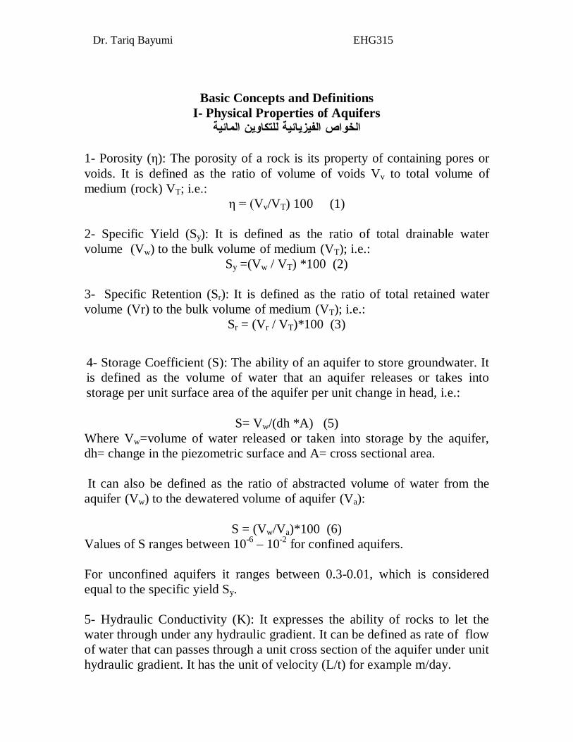
4-Rate of discharge معدل تصريف البئر (Q) The volume of water abstracted during a unit of time. Q has a dimension of volume/ time i.e. m3/day or l/min. 5- Cone of depression مخروط االنخفاض A cone of occurs in an aquifer when ground water is pumped from a well. In an unconfined (water table) aquifer, this is an actual depression of the


water levels. In confined (artesian) aquifers, the cone of depression is a reduction in the pressure head surrounding the pumped well

6- Radius of influence (R) نصف قطر التأثير The radial distance from the center of a well to the point where there is no lowering of the water table or potentiometric surface (the edge of the cone of depression) (m).


قوانين حركة المياه الجوفية Groundwater Flow Laws

Darcy's Law

Darcy law states that the rate of flow through a porous medium is proportional to the loss of head and inversely proportional to the length of the flow path, or

v =Q/A or

v=- Ki= K (∆h/∆L ) =- K (h2-h1/L) where: v = Darcy velocity , Specific discharge , Filter velocity (L/T), A= cross sectional area normal to flow direction (L3). K= Hydraulic conductivity (Coefficient of permeability) (L/T), ∆h= head loss (L), L= distance between two points along the flow path (L), i = dh/dl=h2-h1= Hydraulic gradient is simply the slope of the water table or potentiometric surface. It is the change in hydraulic head over the change in distance between the two monitoring wells. .

Validiy of Darcy's Law

Darcy law is valid only for laminar flow, but not for turbulent flow. In case of doubt, one can use the Reynold's number (NR) as a criterion to distinguish between laminar and turbulent flow. NR is expressed as:

NR = ( ρ vD/μ) Where: NR= Reynold’s No., Ρ= the fluid density, v= the specific discharge, D= the average length of the aquifer material, expressed usually as d10. μ = the fluid viscosity. Darcy law is valid for NR=1- 10.


w

General Groundwater Flow Equations A- Rectangular Coordinates:

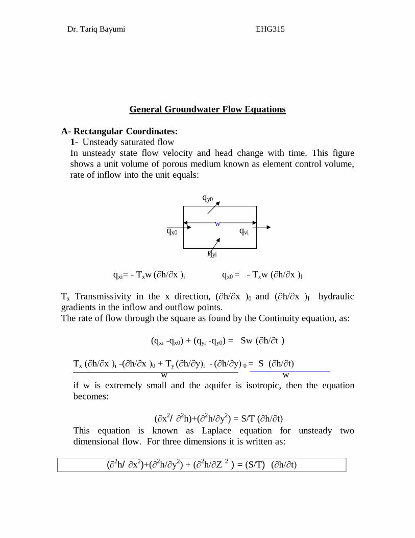
1- Unsteady saturated flow In unsteady state flow velocity and head change with time. This figure shows a unit volume of porous medium known as element control volume, rate of inflow into the unit equals:

qy0

qx0 qvi

qyi

qxi= - Txw (∂h/∂x )i qx0 = - Txw (∂h/∂x )I

Tx Transmissivity in the x direction, (∂h/∂x )0 and (∂h/∂x )I hydraulic gradients in the inflow and outflow points. The rate of flow through the square as found by the Continuity equation, as:

)(∂h/∂t (qxi -qx0) + (qyi -qy0) = Sw

Tx (∂h/∂x )i -(∂h/∂x )0 + Ty (∂h/∂y)i - (∂h/∂y) 0 = S (∂h/∂t) w w if w is extremely small and the aquifer is isotropic, then the equation becomes:

(∂x2 / ∂2h)+(∂2h/∂y2) = S/T (∂h/∂t) This equation is known as Laplace equation for unsteady two dimensional flow. For three dimensions it is written as:

(∂h/∂t) )(S/T ) =2 +(∂2h/∂y2) + (∂2h/∂Z)∂x2 /∂2h(


2- Steady State Flow In steady state flow head does not change with time i.e. ∂h/∂t=0, therefore the above equation becomes:

0 ) =2 +(∂2h/∂y2) + (∂2h/∂Z)∂x2 /∂2h ( B- Radial Coordinates Groundwater flow towards wells is radial. Assuming homogenous and isotropic aquifer Lapalce equation for unsteady state radial flow is:

(∂2h/∂r2) + (1/r)( ∂h/∂r) = (S/T)( ∂h/ ∂t) Laplace equation for steady state radial flow is:

+ (1/r)( ∂h/∂r) = 0 )∂r2/∂2h(


Groundwater Hydraulics and Pumping Tests

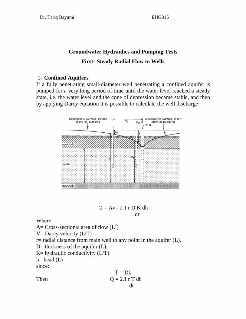
First- Steady Radial Flow to Wells 1- Confined Aquifers If a fully penetrating small-diameter well penetrating a confined aquifer is pumped for a very long period of time until the water level reached a steady state, i.e. the water level and the cone of depression became stable, and then by applying Darcy equation it is possible to calculate the well discharge:

Q = Av= 2Л r D K dh dr Where: A= Cross-sectional area of flow (L2) V= Darcy velocity (L/T) r= radial distance from main well to any point in the aquifer (L), D= thickness of the aquifer (L). K= hydraulic conductivity (L/T). h= head (L) since:

T = Dk Then Q = 2Л r T dh dr


By arranging and integrating: ∂r/r =(2 ЛT/Q) ∂h

∫ ∂r/r =2 Л T /Q ∫∂h ln r2/r1 = 2 Л T /Q (h2-h1)

Q = 2 Л T [h2-h1]

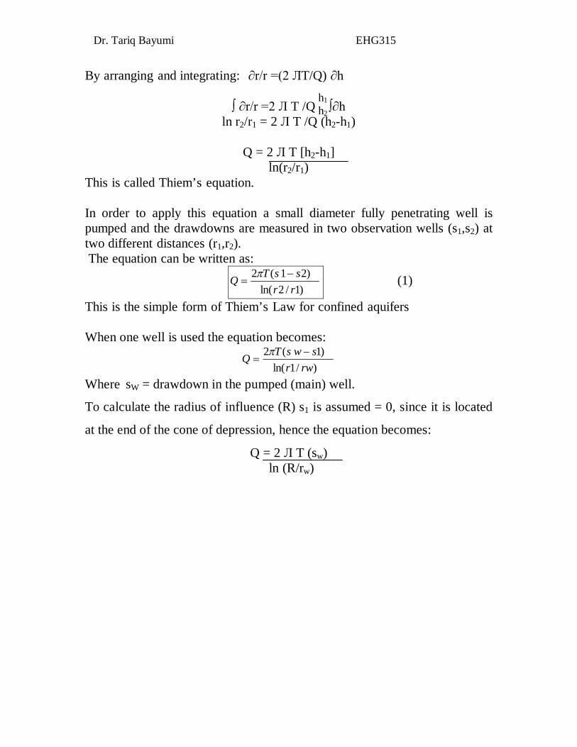
ln(r2/r1) This is called Thiem’s equation. In order to apply this equation a small diameter fully penetrating well is pumped and the drawdowns are measured in two observation wells (s1,s2) at two different distances (r1,r2). The equation can be written as:

)1/2ln(

)21(2rrssTQ

(1)

This is the simple form of Thiem’s Law for confined aquifers

When one well is used the equation becomes:

)/1ln()1(2

rwrswsTQ

Where sW = drawdown in the pumped (main) well.

To calculate the radius of influence (R) s1 is assumed = 0, since it is located

at the end of the cone of depression, hence the equation becomes:

Q = 2 Л T (sw) ln (R/rw)

r

h1 h2


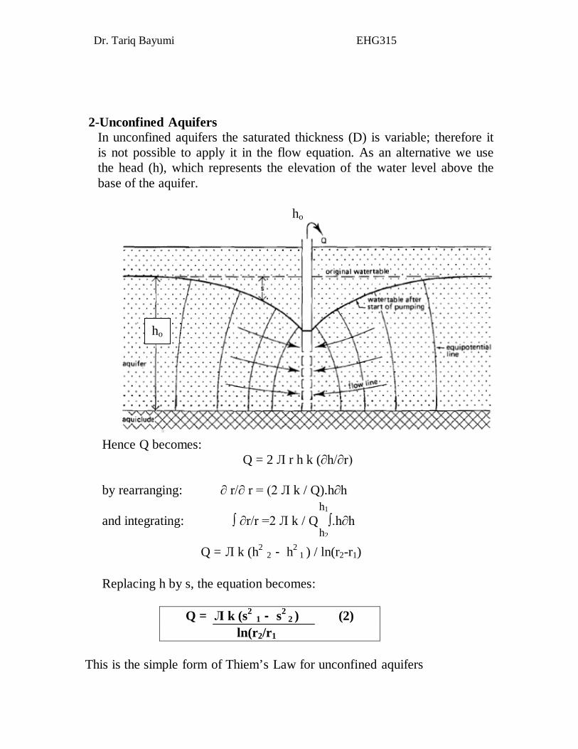
2-Unconfined Aquifers

In unconfined aquifers the saturated thickness (D) is variable; therefore it is not possible to apply it in the flow equation. As an alternative we use the head (h), which represents the elevation of the water level above the base of the aquifer.

ho

Hence Q becomes:

Q = 2 Л r h k (∂h/∂r) by rearranging: ∂ r/∂ r = (2 Л k / Q).h∂h

and integrating: ∫ ∂r/r =2 Л k / Q ∫.h∂h

h2 1

) / ln(r2-r1) - 2 Л k (h2 Q =

Replacing h by s, the equation becomes:

s2 2 ) (2) - 1 Л k (s2 Q =

ln(r2/r1 This is the simple form of Thiem’s Law for unconfined aquifers

h1

h2

ho


If the well suffers from large drawdown compared to the saturated thickness of the aquifer (ho), then transmissivity (T) becomes nearly equal to:

T = k ho

Therefore equation 2 becomes;

T = Q (ln r2/r1)

2 Л [s1-(s21/2 ho)]- [s2-(s2

2 /2 ho)]

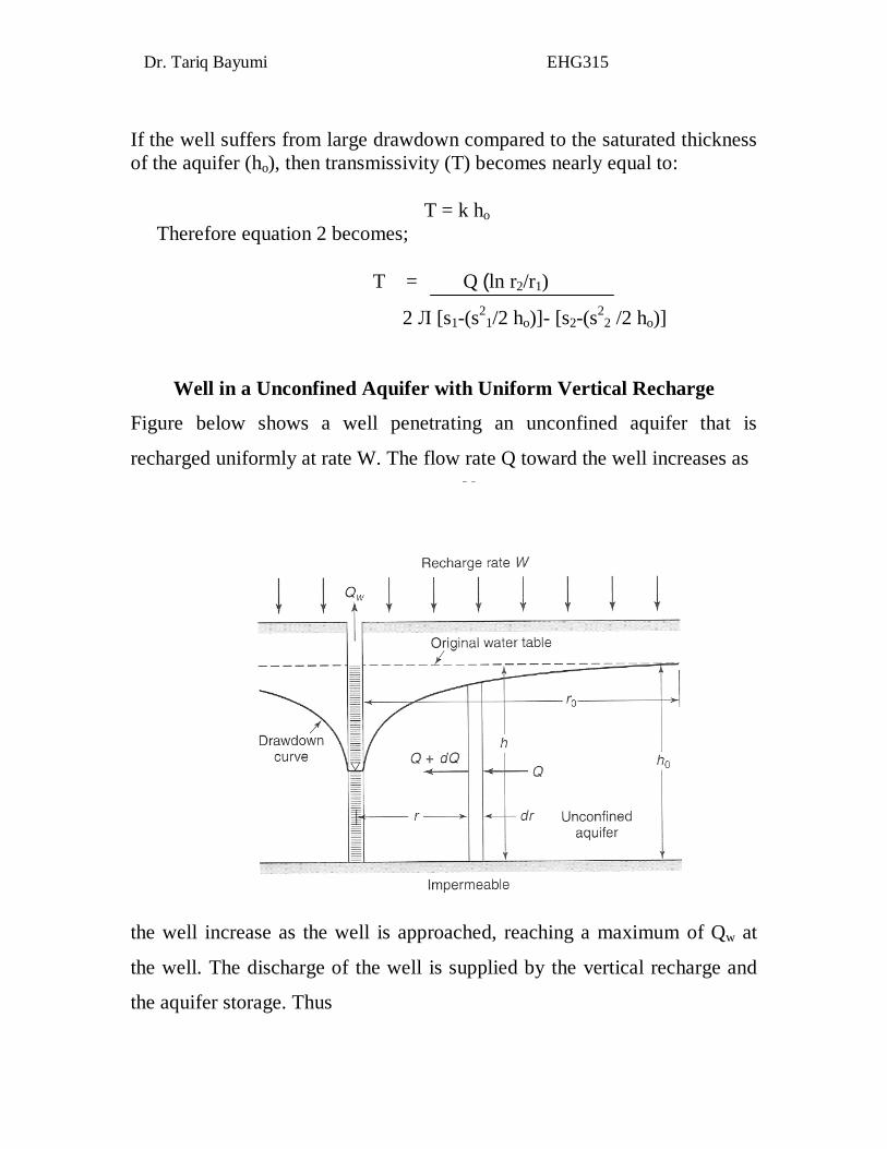
Well in a Unconfined Aquifer with Uniform Vertical Recharge

Figure below shows a well penetrating an unconfined aquifer that is

recharged uniformly at rate W. The flow rate Q toward the well increases as

the well increase as the well is approached, reaching a maximum of Qw at

the well. The discharge of the well is supplied by the vertical recharge and

the aquifer storage. Thus


Q= πr2W+2πrhk(dh/dr) (1)

Integrating, and noting that h=h0 at r=r0, yield the equation for the drawdown

curve:

h0-h2 =W (r2-r02)+Qw ln r0 (2)

2K πK r

By comparing this Thiem equation the effect of vertical recharge becomes apparent. It follows that when r= r0 Q=0, so that equation 1 becomes:

Q= πr02W

Thus the total flow of the well equals the recharge within the circle defined by the radius of influence, which means that the radius of influence is controlled by the well pumping and the recharge rate only. This results in a steady- state drawdown.

Relationship between Discharge and Drawdown in Steady-State Flow

Water level drawdown in wells depends on the rate of discharge. It is possible to make a relationship between the drawdown values of groundwater levels and the discharge of wells penetrating either confined or unconfined aquifers. Specific Capacity (discharge / drawdown Qs): is defined as the amount of well discharge per one meter drop in the groundwater level.

Qs=Q/sw 1- In confined aquifers- according to Thiem equation:

Q/sw= 2ПT/ln(R/rw) 2- In unconfined aquifers

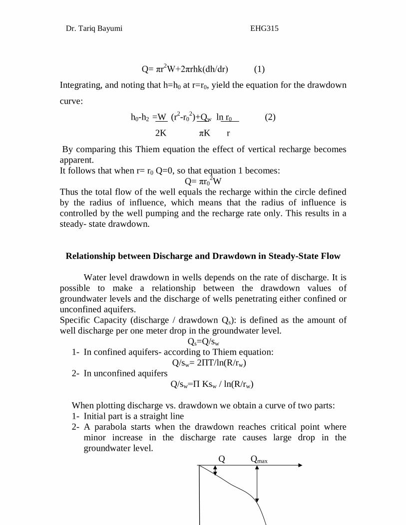
Q/sw=П Ksw / ln(R/rw) When plotting discharge vs. drawdown we obtain a curve of two parts: 1- Initial part is a straight line 2- A parabola starts when the drawdown reaches critical point where

minor increase in the discharge rate causes large drop in the groundwater level.

Q Qmax


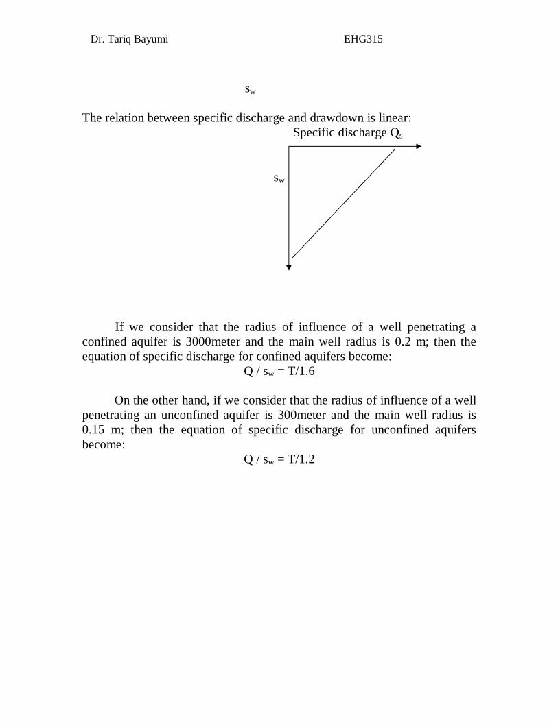
sw

The relation between specific discharge and drawdown is linear: Specific discharge Qs

sw

If we consider that the radius of influence of a well penetrating a confined aquifer is 3000meter and the main well radius is 0.2 m; then the equation of specific discharge for confined aquifers become:

Q / sw = T/1.6 On the other hand, if we consider that the radius of influence of a well penetrating an unconfined aquifer is 300meter and the main well radius is 0.15 m; then the equation of specific discharge for unconfined aquifers become:

Q / sw = T/1.2


Second -Unsteady- State Radial Flow ثانيا: السريان الشعاعي الغيرمستقر

Theis's Method

Theis (1935) was the first to develop a formula for unsteady-state

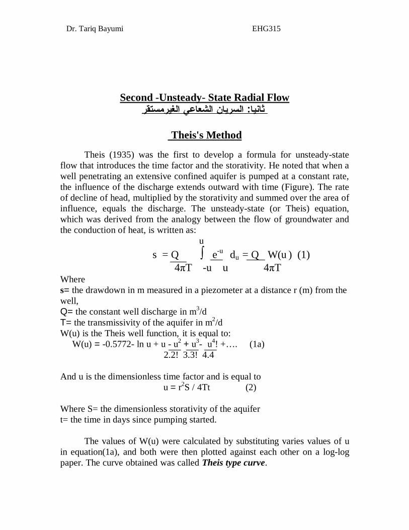
flow that introduces the time factor and the storativity. He noted that when a well penetrating an extensive confined aquifer is pumped at a constant rate, the influence of the discharge extends outward with time (Figure). The rate of decline of head, multiplied by the storativity and summed over the area of influence, equals the discharge. The unsteady-state (or Theis) equation, which was derived from the analogy between the flow of groundwater and the conduction of heat, is written as:

u s = Q ∫ e-u du

= Q W(u ) (1)

4πT -u u 4πT Where s= the drawdown in m measured in a piezometer at a distance r (m) from the well, Q= the constant well discharge in m3/d T= the transmissivity of the aquifer in m2/d W(u) is the Theis well function, it is equal to:

W(u) = -0.5772- ln u + u - u2 + u3- u4! +…. (1a) 2.2! 3.3! 4.4

And u is the dimensionless time factor and is equal to u = r2S / 4Tt (2) Where S= the dimensionless storativity of the aquifer t= the time in days since pumping started.

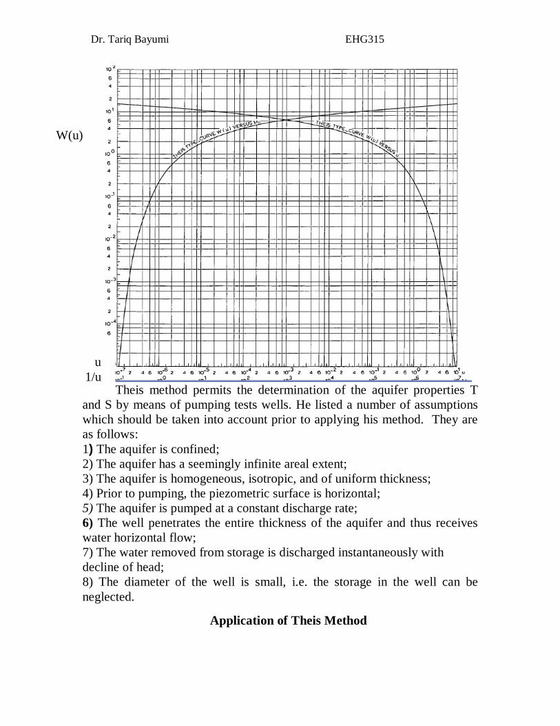
The values of W(u) were calculated by substituting varies values of u

in equation(1a), and both were then plotted against each other on a log-log paper. The curve obtained was called Theis type curve.


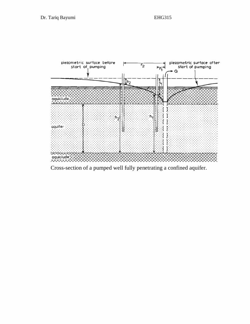
Cross-section of a pumped well fully penetrating a confined aquifer.


Theis method permits the determination of the aquifer properties T

and S by means of pumping tests wells. He listed a number of assumptions which should be taken into account prior to applying his method. They are as follows: 1) The aquifer is confined; 2) The aquifer has a seemingly infinite areal extent; 3) The aquifer is homogeneous, isotropic, and of uniform thickness; 4) Prior to pumping, the piezometric surface is horizontal; 5) The aquifer is pumped at a constant discharge rate; 6) The well penetrates the entire thickness of the aquifer and thus receives water horizontal flow; 7) The water removed from storage is discharged instantaneously with decline of head; 8) The diameter of the well is small, i.e. the storage in the well can be neglected.

Application of Theis Method

W(u)

u 1/u


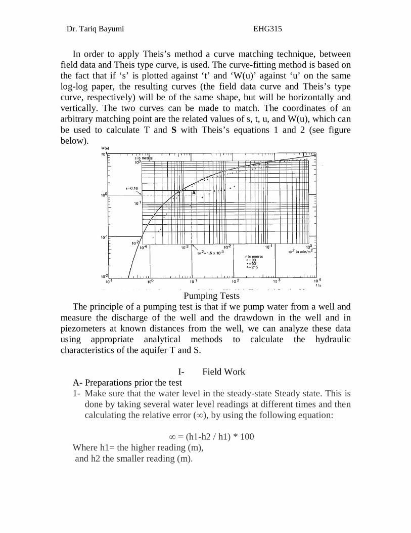
In order to apply Theis’s method a curve matching technique, between field data and Theis type curve, is used. The curve-fitting method is based on the fact that if ‘s’ is plotted against ‘t’ and ‘W(u)’ against ‘u’ on the same log-log paper, the resulting curves (the field data curve and Theis’s type curve, respectively) will be of the same shape, but will be horizontally and vertically. The two curves can be made to match. The coordinates of an arbitrary matching point are the related values of s, t, u, and W(u), which can be used to calculate T and S with Theis’s equations 1 and 2 (see figure below).

Pumping Tests

The principle of a pumping test is that if we pump water from a well and measure the discharge of the well and the drawdown in the well and in piezometers at known distances from the well, we can analyze these data using appropriate analytical methods to calculate the hydraulic characteristics of the aquifer T and S.

I- Field Work

A- Preparations prior the test 1- Make sure that the water level in the steady-state Steady state. This is

done by taking several water level readings at different times and then calculating the relative error (∞), by using the following equation:

∞ = (h1-h2 / h1) * 100

Where h1= the higher reading (m), and h2 the smaller reading (m).


If ∞ is equal to 5% or less, then we can consider the flow is in steady condition. If not then we must wait until it becomes constant. 2 -Measure the static water level. 3- Measure the total depth of the well. 4 - Measure the diameter of the well and the distance between the main well and observation wells, if available. 5 – Prepare the stopwatch and the data sheet to register the data.

B- Conducting the Pumping Test: 1- Start the pump at moderate speed. 2- Start the stop watch as soon as you started pumping. 3- Measure the water level in the well at certain intervals of time and

write the measure data on the data sheet (see table). 4- Measure the well discharge (Q) several times and take their average. 5- When the water level becomes stable stop the pump, and start

measuring the water level recovery. 6 – Plot the time-drawdown data on log-log and semi-log sheets. C- Necessary equipment for the pumping test: 1 – One main (pumped) well and one or two observation wells (or piezometers), 2 – A pump

3-One or two stop watches, 4-A tape Meter, .5 - A device for measuring the depth to the water level, 6- A device for measuring the rate of discharge of the well.

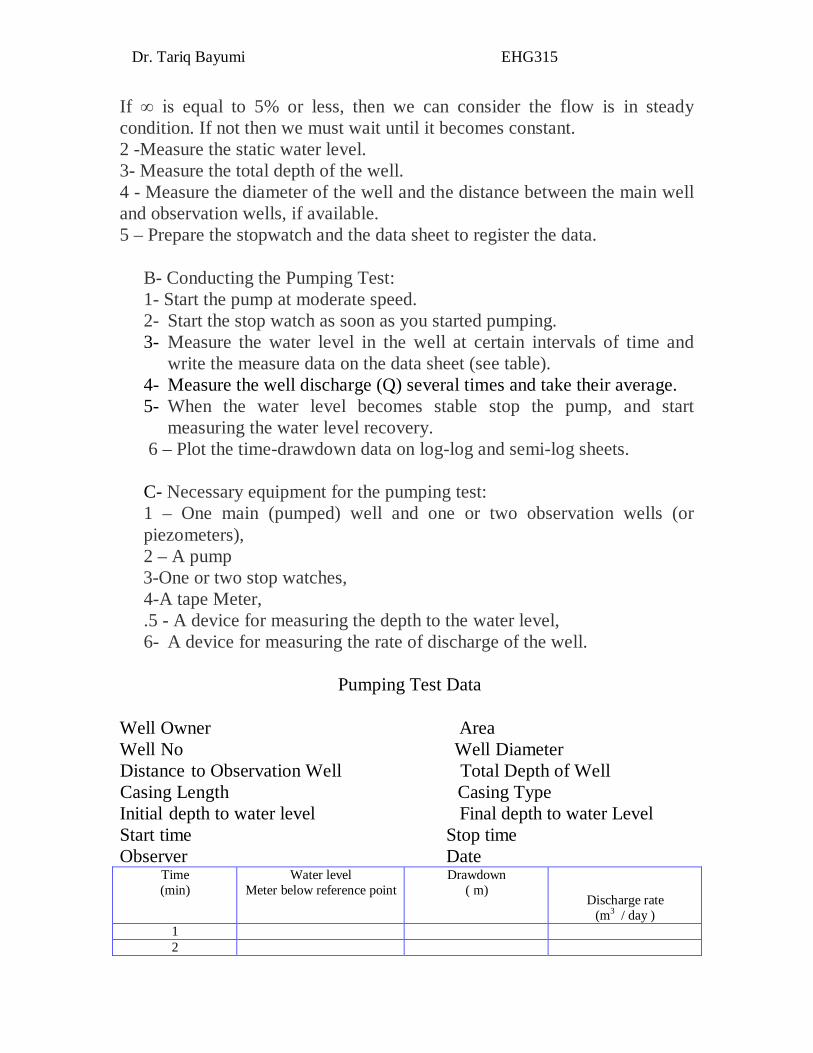
Pumping Test Data

Well Owner Area Well No Well Diameter

Total Depth of Well to Observation Well Distance Casing Length Casing Type Initial depth to water level Final depth to water Level Start time Stop time Observer Date

Discharge rate

(m3 / day )

Drawdown ( m)

Water level Meter below reference point

Time (min)

1 2


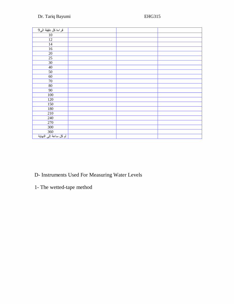
9قراءة كل دقيقة الى 10 12 14 16 20 25 30 40 50 60 70 80 90 100 120 150 180 210 240 270 300 360 ثم كل ساعة إلى النهاية

D- Instruments Used For Measuring Water Levels 1- The wetted-tape method


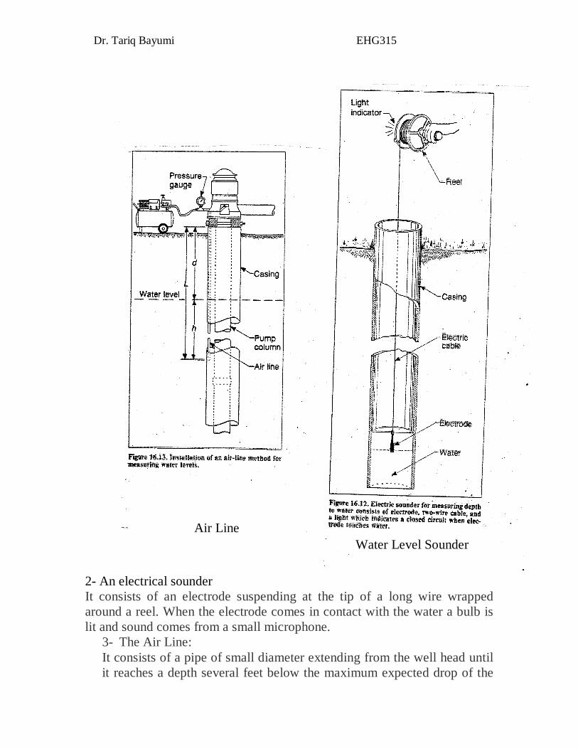
2- An electrical sounder It consists of an electrode suspending at the tip of a long wire wrapped around a reel. When the electrode comes in contact with the water a bulb is lit and sound comes from a small microphone.

3- The Air Line: It consists of a pipe of small diameter extending from the well head until it reaches a depth several feet below the maximum expected drop of the

Water Level Sounder

Air Line


water level. The length of the pipe must be known accurately. The pipe is connected through a T-shaped link to a pressure meter, which measures the pressure in the pipe. The measured pressure is usually in foot. The system is designed so that the pressure needed to push all the water out of the submerged part of the tube is equal to the air pressure of a column of water that has the same height. If the pressure is in foot, then it is possible to calculate the depth of the water level in the well, by the following equation:

D = L-H Where: D = depth of the water level in foot, L = depth to the end of the air line, H = the measured pressure in foot, represented by a water column height equal to the length of the submersed part of the air line.

E- Instruments Used For Measuring Well Discharge

1-Use a known volume container and a Stopwatch: A simple and accurate way to measure the rate of pumping is to fill a container of known volume with water and determining the time needed to fill it. 2 - Water Meter:

The commercial water meter (commonly use at homes) can be used to measure the volume of water that is pumped in a given period of time. 3 -Circular orifice weir:

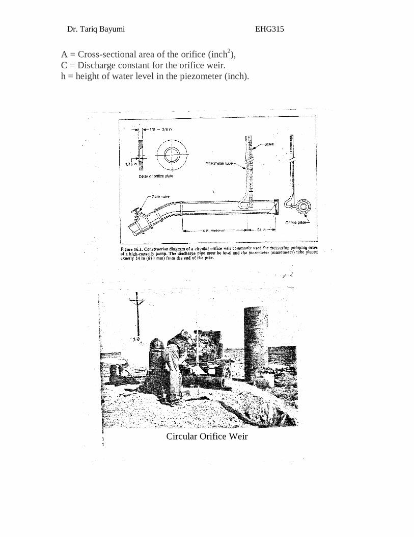
It consists of a round slab of steel with a circular hole in the center. The orifice weir is about 1 / 16 inch thick. It is usually fitted at the end of a horizontal discharge pipe 6 feet long. A hole is pierced in the horizontal pipe 24 inches ahead of the weir and a transparent pipe (piezometric tube) is fitted in the hole. When water is pumped through the weir, the height of the water in the piezometer represents the pressure inside the discharge pipe.

Special tables are used to determine the flow rate in gallon / min for different diameters of both the weir and the discharge pipes. The discharge is calculated using the following equation:

Q = 8.02AC √ h

Where: Q = Discharge per unit time (gallon/min),


A = Cross-sectional area of the orifice (inch2), C = Discharge constant for the orifice weir. h = height of water level in the piezometer (inch).

Circular Orifice Weir


II- Office Work The time-drawdown plots obtained from the pumping tests are plotted on semi-logarithmic and /or log-lag papers. Each plot serves certain purposes: 1. Semi-logarithmic paper: When using semi-log papers the pumping test data fall along straight lines. They benefit the following purposes: a- Determining the characteristics of the aquifers (T and S) using straight-line methods. b- Indicating the well-diameter effect. C -Determining the well loss. D – Indicating the possibility of application of Darcy law. 2. Logarithmic paper: Log-log paper When using log-log papers the pumping test data form curves. They benefit the following purposes:

a- Determine the aquifer characteristics (T &S) of the water-bearing layer by curve matching techniques.

b- Estimating the nature of the homogeneity of aquifer. c- If the initial readings fill on a straight line, the well has a large

diameter well. d- If the final readings fill on a straight line, the aquifer is fractured. e- Determining the aquifer type from the shape of the curve.


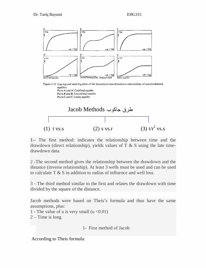
Jacob Methodsطرق جاكوب

(1) t vs.s (2) s vs.r (3) t/r2 vs.s 1-- The first method: indicates the relationship between time and the drawdown (direct relationship), yields values of T & S using the late time-drawdown data. 2 -The second method gives the relationship between the drawdown and the distance (inverse relationship). At least 3 wells must be used and can be used to calculate T & S in addition to radius of influence and well loss. 3 - The third method similar to the first and relates the drawdown with time divided by the square of the distance. Jacob methods were based on Theis’s formula and thus have the same assumptions, plus: 1 - The value of u is very small (u <0.01) 2 – Time is long.

1- First method of Jacob

According to Theis formula:


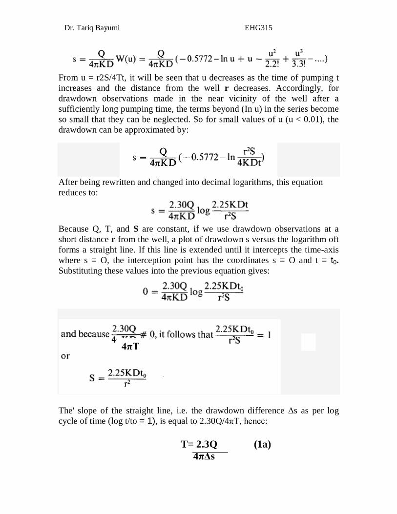
From u = r2S/4Tt, it will be seen that u decreases as the time of pumping t increases and the distance from the well r decreases. Accordingly, for drawdown observations made in the near vicinity of the well after a sufficiently long pumping time, the terms beyond (In u) in the series become so small that they can be neglected. So for small values of u (u < 0.01), the drawdown can be approximated by:

After being rewritten and changed into decimal logarithms, this equation reduces to:

Because Q, T, and S are constant, if we use drawdown observations at a short distance r from the well, a plot of drawdown s versus the logarithm oft forms a straight line. If this line is extended until it intercepts the time-axis where s = O, the interception point has the coordinates s = O and t = t0. Substituting these values into the previous equation gives:

The' slope of the straight line, i.e. the drawdown difference Δs as per log cycle of time (log t/to = 1), is equal to 2.30Q/4πT, hence:

T= 2.3Q (1a) 4πΔs

4πT 2


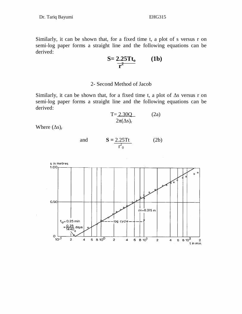
Similarly, it can be shown that, for a fixed time t, a plot of s versus r on semi-log paper forms a straight line and the following equations can be derived:

S= 2.25Tto (1b) r2

2- Second Method of Jacob

Similarly, it can be shown that, for a fixed time t, a plot of Δs versus r on semi-log paper forms a straight line and the following equations can be derived: T= 2.30Q (2a)

2π(Δs)r Where (Δs)r

and S = 2.25Tt (2b)

r20


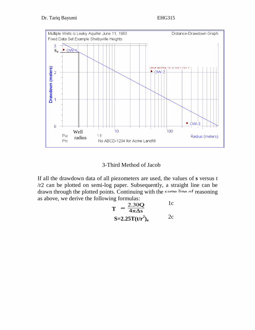
The well Loss The well loss indicates the difference between the groundwater level within the well and the area surrounding the well; this difference occurs as a result of the deterioration of the well efficiency due to clogging of well screen by fine sediments. The well loss is inversely proportional with the aquifer permeability and the well radius.

Determining the well loss

1 - Plot the pumping test data (drawdown vs. distance) on a semi log paper and draw a straight line through the points. 2 – Locate the point representing the well radius on the distance axis and extend a vertical line from that point till it intersects with the data straight line. Draw a horizontal line from the point of intersection until intersects with the drawdown axis. The intersection point on s axis represents the drawdown in the circulating the well.(sa). 3- Determine the well loss (Wl) from the relation:

Wl=sw-sa Where sw the drawdown measured inside the well itself.


3-Third Method of Jacob

If all the drawdown data of all piezometers are used, the values of s versus t /r2 can be plotted on semi-log paper. Subsequently, a straight line can be drawn through the plotted points. Continuing with the same line of reasoning as above, we derive the following formulas:

S=2.25T(t/r2)o

1c 2c

Well radius

sa

T


Slope- Matching Method طريقة الميل

Sen (1986) developed this method, which has the following characteristics: 1 - Early data as well as late data can be used in the analysis and either can be omitted. 2 – The method gives a series of values of S, T and on the basis of these values it is possible to estimate the homogeneity of the aquifer. 3 - No plotting is required for the time-drawdown data. Assumptions of this method are the same as those of Theis; however it does not require the homogeneity of aquifer water.

Theory

Sen found that it is possible to calculate the slope of the Theis type curve at any point by the equation: ∞ = - e-u (1) W (u) It was then possible to prepare a table relating the values of u to the corresponding values of slope (∞); with the help of this table one can calculate the hydraulic characteristics of the aquifer using pumping test data as follows:

Procedure

1 – Calculate the slope between the first two sets of data (∞i) for the time vs. drawdown using the following equation:

∞i = [log (si / si-1)] / [log (ti-1/ti)] (2) Where: i = 1,2,3,4,.., n, and n represents the number of readings of time vs. drawdown. Applying equation 2 on the first two sets of data yields:

∞i = [log (s2 / s1)] / [log (t1 / t2)] (3)

Note that the slope values are always negative.


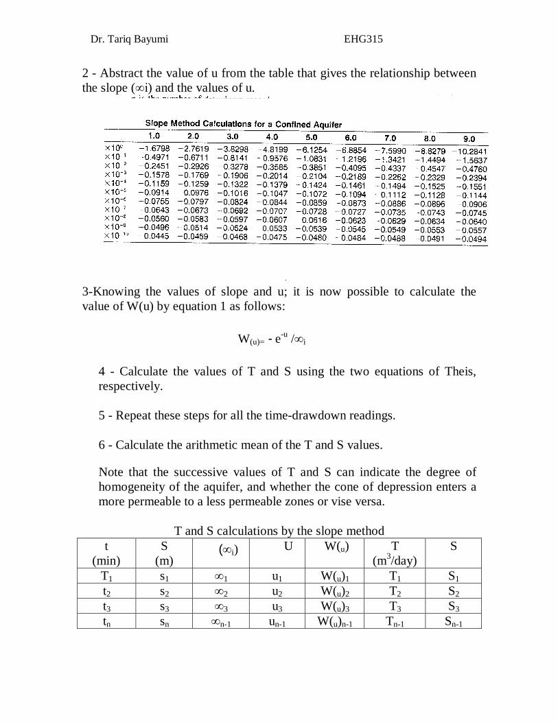
2 - Abstract the value of u from the table that gives the relationship between the slope (∞i) and the values of u.

3-Knowing the values of slope and u; it is now possible to calculate the value of W(u) by equation 1 as follows:

e-u /∞i - W(u)=

4 - Calculate the values of T and S using the two equations of Theis, respectively. 5 - Repeat these steps for all the time-drawdown readings. 6 - Calculate the arithmetic mean of the T and S values. Note that the successive values of T and S can indicate the degree of homogeneity of the aquifer, and whether the cone of depression enters a more permeable to a less permeable zones or vise versa.

T and S calculations by the slope method

S T (m3/day)

W(u) U )∞i( S (m)

t (min)

S1 T1 W(u)1 u1 ∞1 s1 T1 S2 T2 W(u)2 u2 ∞2 s2 t2 S3 T3 W(u)3 u3 ∞3 s3 t3

Sn-1 Tn-1 W(u)n-1 un-1 ∞n-1 sn tn


Large-Diameter Wells اآلبار ذات األقطار الكبیرة

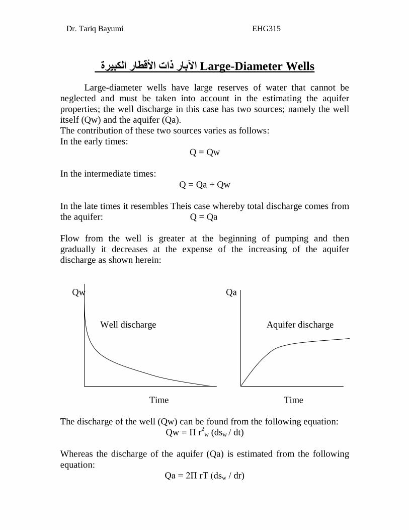
Large-diameter wells have large reserves of water that cannot be

neglected and must be taken into account in the estimating the aquifer properties; the well discharge in this case has two sources; namely the well itself (Qw) and the aquifer (Qa). The contribution of these two sources varies as follows: In the early times:

Q = Qw In the intermediate times:

Q = Qa + Qw In the late times it resembles Theis case whereby total discharge comes from the aquifer: Q = Qa Flow from the well is greater at the beginning of pumping and then gradually it decreases at the expense of the increasing of the aquifer discharge as shown herein: Qw Qa Well discharge Aquifer discharge Time Time The discharge of the well (Qw) can be found from the following equation:

Qw = Π r2w (dsw / dt)

Whereas the discharge of the aquifer (Qa) is estimated from the following equation:

Qa = 2Π rT (dsw / dr)


The additional source of discharge contrasts with one of Theis’s method assumptions, and therefore it is not possible to apply it on pumping tests data obtained from such wells.

Papadopulos Method, 1967 طريقة بابادوبولس وكوبر This method was built on Theis’s assumptions with the exception that: 1. The well diameter is not small; hence, storage in the well cannot be neglected; 2 - The well loss is small. For unsteady-state flow to a fully penetrating, large-diameter well in a confined aquifer Papadopulos (1967) gives the following drawdown equation:

1)( F(uw ,β) T = Q 4 Л sw

Where uw= r2

w S (2) 4Tt and β= r2

w S (3) r2

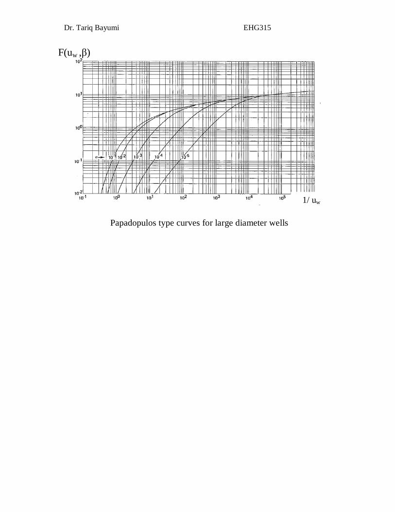
c F(uw ,β) is the well function of Papadopulos, rc= effective radius of the well screen or open hole, rw= radius of the unscreened part of the well over which the water level is changing. Equation 1 has the same form as the Theis well function, but there are two parameters in the integral: uw and β. On the basis of Equation 1, Papadopulos (1967) developed a modification of the Theis curve-fitting method, but instead of using one type curve, he uses a type curve for each value of β (see below). We can match the pumping test data curves with these type curves to calculate the properties of water-bearing layer with the help of equations 1 and 2. The type curves consist of three parts:


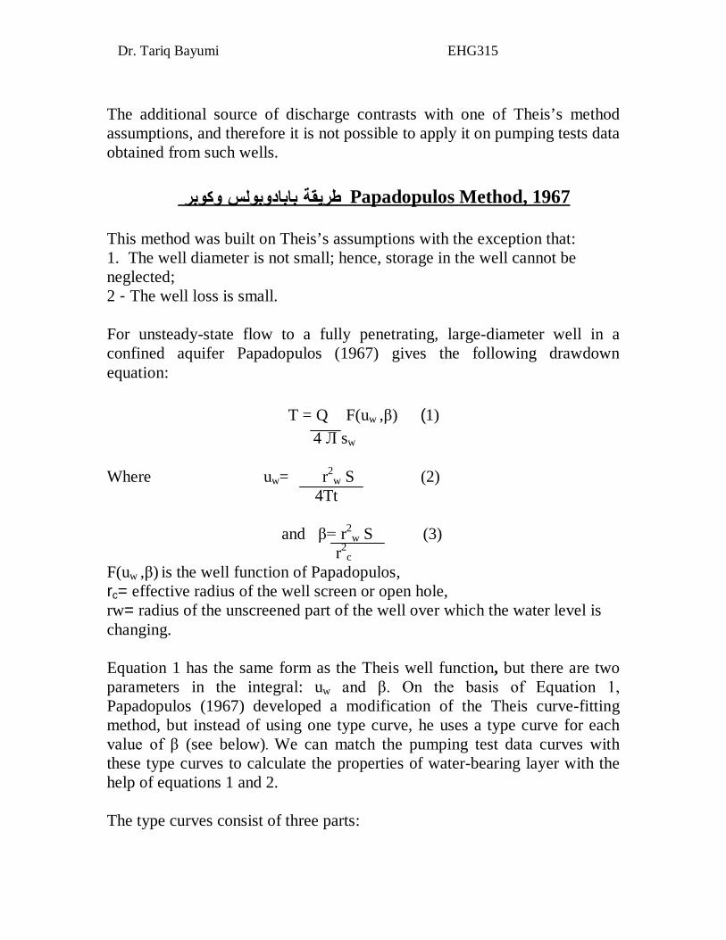
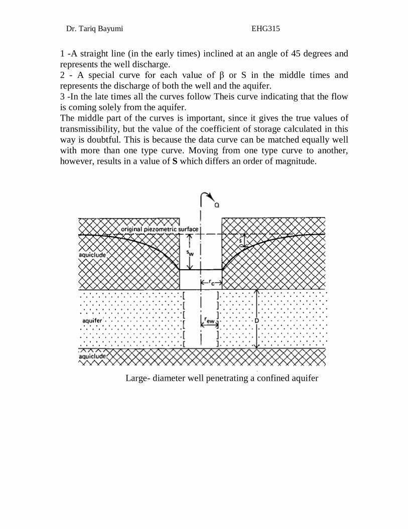
1 -A straight line (in the early times) inclined at an angle of 45 degrees and represents the well discharge. 2 - A special curve for each value of β or S in the middle times and represents the discharge of both the well and the aquifer. 3 -In the late times all the curves follow Theis curve indicating that the flow is coming solely from the aquifer. The middle part of the curves is important, since it gives the true values of transmissibility, but the value of the coefficient of storage calculated in this way is doubtful. This is because the data curve can be matched equally well with more than one type curve. Moving from one type curve to another, however, results in a value of S which differs an order of magnitude.

Large- diameter well penetrating a confined aquifer


F(uw ,β)

Papadopulos type curves for large diameter wells

1/ uw


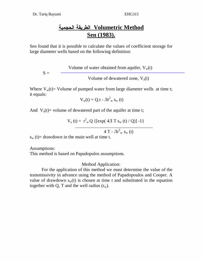
Volumetric Method الطريقة الحجمية Sen (1983).

Sen found that it is possible to calculate the values of coefficient storage for large diameter wells based on the following definition: Volume of water obtained from aquifer, Vw(t) S =

Volume of dewatered zone, Va(t) Where Vw(t)= Volume of pumped water from large diameter wells at time t; it equals:

Vw(t) = Q.t - Лr2w sw (t)

And Va(t)= volume of dewatered part of the aquifer at time t;

Va (t) = r2

w Q {[exp( 4Л T sw (t) / Q)] -1}

4 T - Лr2w sw (t)

sw (t)= drawdown in the main well at time t. Assumptions: This method is based on Papadopulos assumptions.

Method Application: For the application of this method we must determine the value of the

transmissivity in advance using the method of Papadopoulos and Cooper. A value of drawdown sw(t) is chosen at time t and substituted in the equation together with Q, T and the well radius (rw).


Discharge Calulation from Early Drawdown Data in Large- Diameter Wells ( Sen , 1986)

حساب قيمة التصريف من اآلبار ذات األقطار الكبيرة باستخدام قراءات االنخفاض المبكر

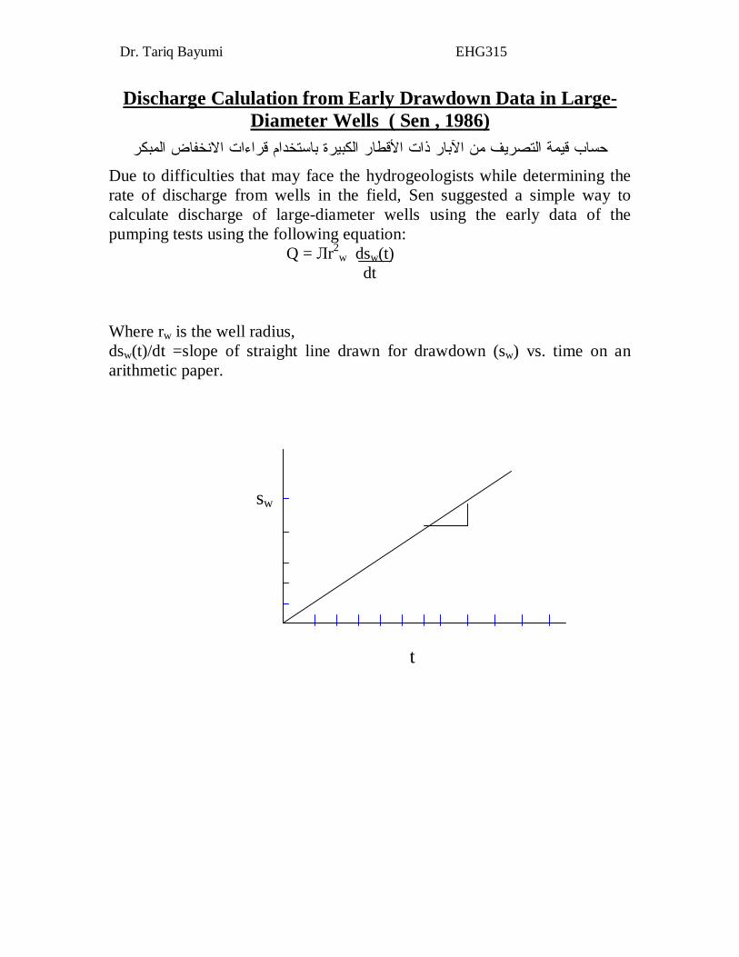
Due to difficulties that may face the hydrogeologists while determining the rate of discharge from wells in the field, Sen suggested a simple way to calculate discharge of large-diameter wells using the early data of the pumping tests using the following equation:

Q = Лr2w dsw(t)

dt Where rw is the well radius, dsw(t)/dt =slope of straight line drawn for drawdown (sw) vs. time on an arithmetic paper.

sw t


Unconfined Aquifers التكاوین المائیة غیر المحصورة

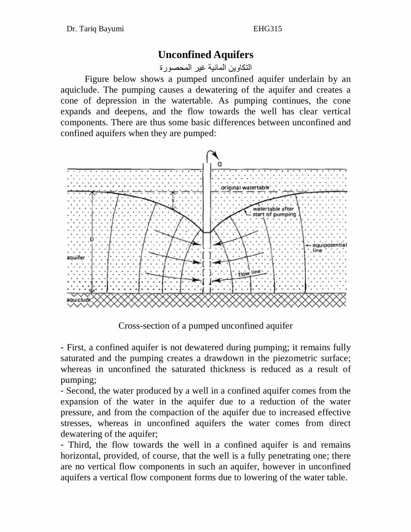
Figure below shows a pumped unconfined aquifer underlain by an aquiclude. The pumping causes a dewatering of the aquifer and creates a cone of depression in the watertable. As pumping continues, the cone expands and deepens, and the flow towards the well has clear vertical components. There are thus some basic differences between unconfined and confined aquifers when they are pumped:

Cross-section of a pumped unconfined aquifer

- First, a confined aquifer is not dewatered during pumping; it remains fully saturated and the pumping creates a drawdown in the piezometric surface; whereas in unconfined the saturated thickness is reduced as a result of pumping; - Second, the water produced by a well in a confined aquifer comes from the expansion of the water in the aquifer due to a reduction of the water pressure, and from the compaction of the aquifer due to increased effective stresses, whereas in unconfined aquifers the water comes from direct dewatering of the aquifer; - Third, the flow towards the well in a confined aquifer is and remains horizontal, provided, of course, that the well is a fully penetrating one; there are no vertical flow components in such an aquifer, however in unconfined aquifers a vertical flow component forms due to lowering of the water table.


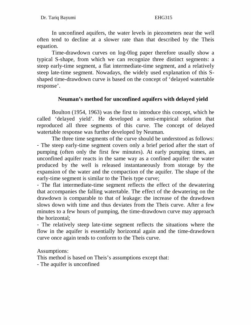
In unconfined aquifers, the water levels in piezometers near the well often tend to decline at a slower rate than that described by the Theis equation.

Time-drawdown curves on log-0log paper therefore usually show a typical S-shape, from which we can recognize three distinct segments: a steep early-time segment, a flat intermediate-time segment, and a relatively steep late-time segment. Nowadays, the widely used explanation of this S-shaped time-drawdown curve is based on the concept of ‘delayed watertable response’.

Neuman’s method for unconfined aquifers with delayed yield

Boulton (1954, 1963) was the first to introduce this concept, which he

called ‘delayed yield’. He developed a semi-empirical solution that reproduced all three segments of this curve. The concept of delayed watertable response was further developed by Neuman.

The three time segments of the curve should be understood as follows: - The steep early-time segment covers only a brief period after the start of pumping (often only the first few minutes). At early pumping times, an unconfined aquifer reacts in the same way as a confined aquifer: the water produced by the well is released instantaneously from storage by the expansion of the water and the compaction of the aquifer. The shape of the early-time segment is similar to the Theis type curve; - The flat intermediate-time segment reflects the effect of the dewatering that accompanies the falling watertable. The effect of the dewatering on the drawdown is comparable to that of leakage: the increase of the drawdown slows down with time and thus deviates from the Theis curve. After a few minutes to a few hours of pumping, the time-drawdown curve may approach the horizontal; - The relatively steep late-time segment reflects the situations where the flow in the aquifer is essentially horizontal again and the time-drawdown curve once again tends to conform to the Theis curve. Assumptions: This method is based on Theis’s assumptions except that: - The aquifer is unconfined


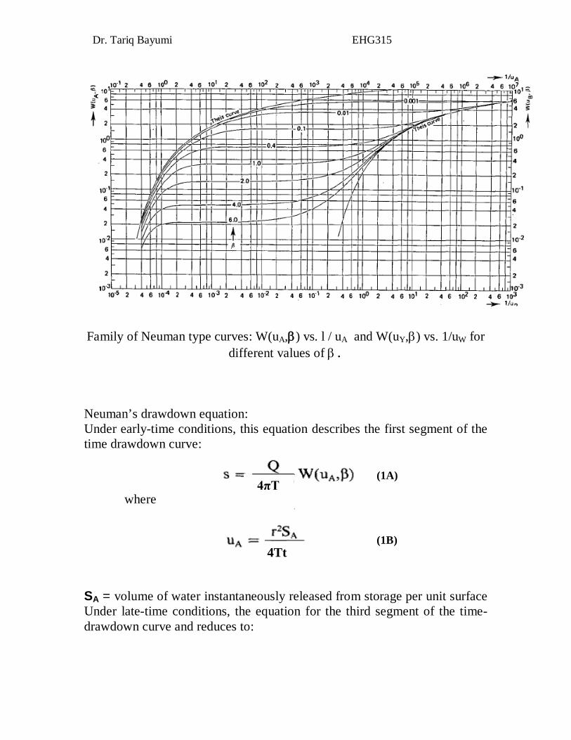
Family of Neuman type curves: W(uA,) vs. l / uA and W(uY,) vs. 1/uW for different values of .

Neuman’s drawdown equation: Under early-time conditions, this equation describes the first segment of the time drawdown curve:

SA = volume of water instantaneously released from storage per unit surface Under late-time conditions, the equation for the third segment of the time-drawdown curve and reduces to:

where

(1A) (1B)

4πT

4Tt


Where:

Sy = volume of water released from storage per unit surface area per unit decline of the watertable, i.e. released by dewatering of the aquifer (= specific yield).

Method Application

Prepare the observed data curve on a transparent sheet of log-log paper of the same scale as that of Numan’s type curves by plotting the values of the drawdown s against the corresponding time t for a single observation well at a distance r from the pumped well; - Match the early-time observed data plot with one of the type A curves. Note the value of the selected type A curve; - Select an arbitrary point A on the overlapping portion of the two sheets and note the values of s, t, l/uA, and W(u, ) for this point; - Substitute these values into Equations 1A and 1B and, knowing Q and r, calculate T and SA; - Move the observed data curve until as many as possible of the late-time observed data fall on the type B curve with the same value as the selected type A curve; - Select an arbitrary point B on the superimposed sheets and note the values of s, t, l/uB, and W(u, ) for this point; - Substitute these values into Equations 2A and 2B and, knowing Q and r, calculate T and Sy. The final storativity S= SA + Sy. However, in situations where the effect of delayed watertable response is clearly evident, SA << Sy, and the influence of SA at larger times can safely be neglected, therefore S=Sy.

2A 2B

4πT

4Tt


Applying methods of confined aquifers on unconfined aquifers

Although the aquifer is assumed to be of uniform thickness, this condition is not met if the drawdown is large compared with the aquifer’s original saturated thickness. A corrected value for the observed drawdown s then has to be applied. Jacob (1 944) proposed the following correction:

s- = s - (s2/2D)

where s- = corrected drawdown; s = observed drawdown; D = original saturated aquifer thickness. Jacob’s correction is strictly applicable only to the late time drawdown data, which fall on the Theis curve.


التكاوین المائیة التھریبیة (شبھ المحصورة) Leaky aquifers (Semi-confined aquifers)

In nature, leaky aquifers occur far more frequently than the perfectly

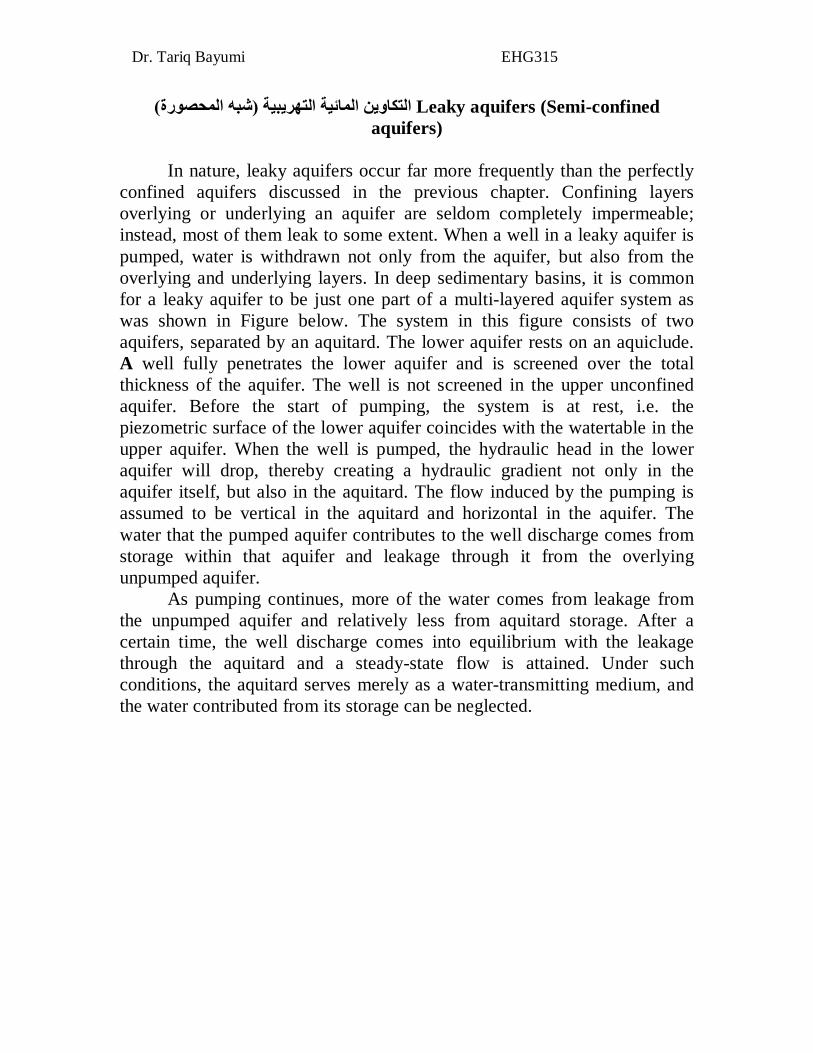
confined aquifers discussed in the previous chapter. Confining layers overlying or underlying an aquifer are seldom completely impermeable; instead, most of them leak to some extent. When a well in a leaky aquifer is pumped, water is withdrawn not only from the aquifer, but also from the overlying and underlying layers. In deep sedimentary basins, it is common for a leaky aquifer to be just one part of a multi-layered aquifer system as was shown in Figure below. The system in this figure consists of two aquifers, separated by an aquitard. The lower aquifer rests on an aquiclude. A well fully penetrates the lower aquifer and is screened over the total thickness of the aquifer. The well is not screened in the upper unconfined aquifer. Before the start of pumping, the system is at rest, i.e. the piezometric surface of the lower aquifer coincides with the watertable in the upper aquifer. When the well is pumped, the hydraulic head in the lower aquifer will drop, thereby creating a hydraulic gradient not only in the aquifer itself, but also in the aquitard. The flow induced by the pumping is assumed to be vertical in the aquitard and horizontal in the aquifer. The water that the pumped aquifer contributes to the well discharge comes from storage within that aquifer and leakage through it from the overlying unpumped aquifer.

As pumping continues, more of the water comes from leakage from the unpumped aquifer and relatively less from aquitard storage. After a certain time, the well discharge comes into equilibrium with the leakage through the aquitard and a steady-state flow is attained. Under such conditions, the aquitard serves merely as a water-transmitting medium, and the water contributed from its storage can be neglected.


Hantush Inflection- Point Method

The assumptions and conditions underlying this method are similar to Theis‘s assumption except that:

- The aquifer is leaky; - The flow is unsteady, however the steady state drawdown must be

known. Hantush (1956) developed the inflection point method. To determine the

inflection point P the steady state drawdown sm, should be known, either from direct observations or from extrapolation. The curve of s versus t on semi-log paper has an inflection point P where the following relations hold

where KO is the modified Bessel function of the second kind and zero order

The slope of the curve at the inflection point Δsp is given by:

4Ttp

4π T (1)

(2)

Leaky aquifer

Unconfined aquifer


At the inflection point, the relation between the drawdown and the slope of the curve is given by:

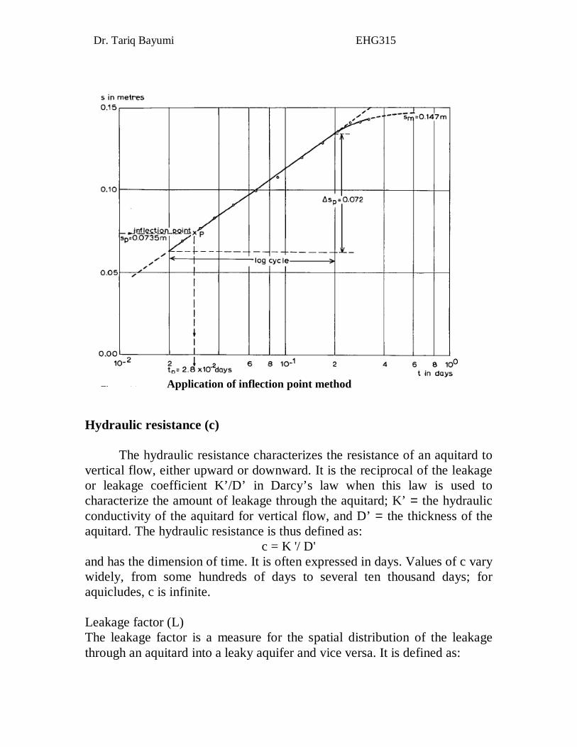
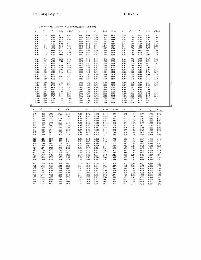
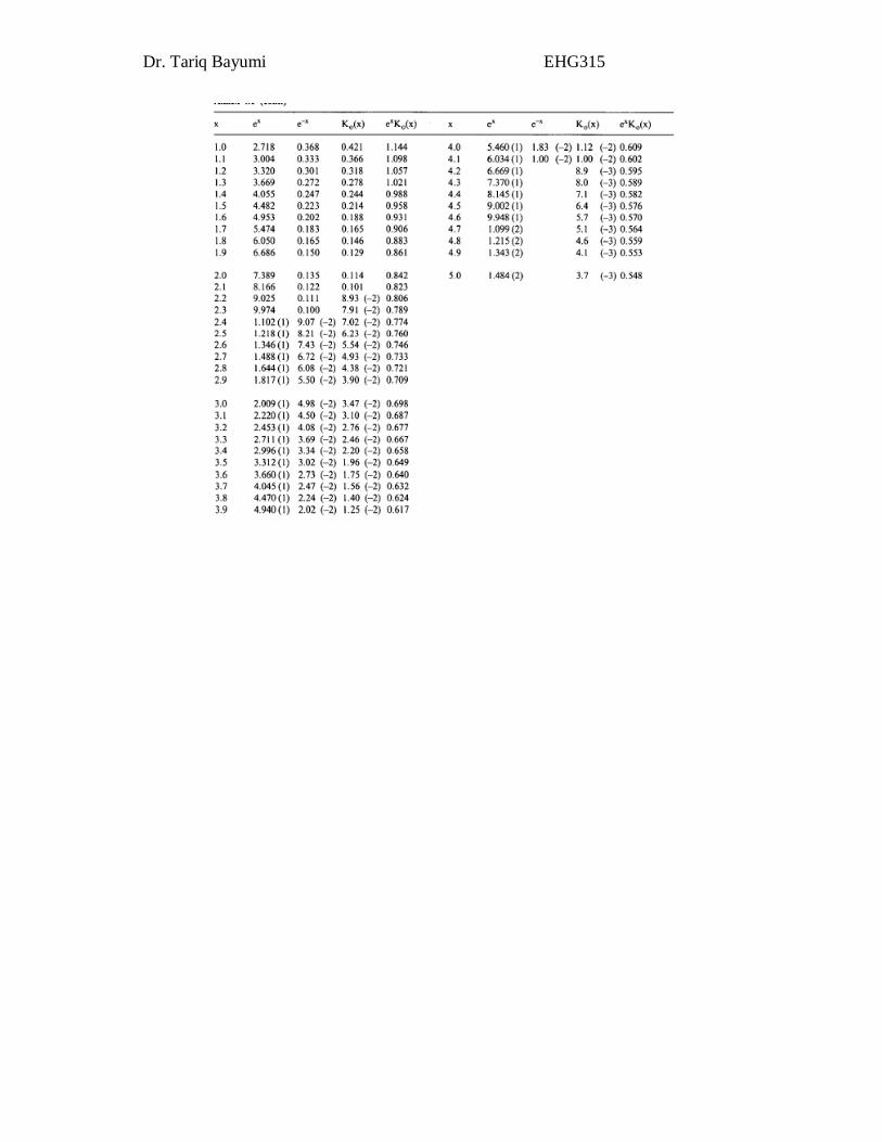
Procedure: 1- Plot s versus t on semi-log paper (t on logarithmic scale) and draw the curve that best fits through the plotted points (see figure below); 2- Determine the value of the maximum drawdown sm, by extrapolation. This is only possible if the period of the test was long enough. 3- Calculate sp, with Equation 1: where sp =0.5sm. The value of sp on the curve locates the inflection point P; 4- Read the value of tp, at the inflection point from the time-axis; 5- Determine the slope Δsp, of the curve at the inflection point. This can be closely approximated by reading the drawdown difference per log cycle of time over the straight portion of the curve on which the inflection point lies, or over the tangent to the curve at the inflection point; 6- Substitute the values of sp, and Δsp into Equation 4 and find r/L by interpolation from a special table of the function eXKo(x ) (See table below); 7- Knowing r/L and r, calculate L; 8- Knowing Q, s,, Asp, and r/L, calculate T from Equation 3, using the table of the function eXKo(x); 9- Knowing T, tP,, r, and r/L, calculate S from Equation:

S=2Ttp r (5)

r2 L 10- Knowing KD and L, calculate c from the relation c = L2/T.

4πT (3)

(4)


Hydraulic resistance (c)

The hydraulic resistance characterizes the resistance of an aquitard to

vertical flow, either upward or downward. It is the reciprocal of the leakage or leakage coefficient K’/D’ in Darcy’s law when this law is used to characterize the amount of leakage through the aquitard; K’ = the hydraulic conductivity of the aquitard for vertical flow, and D’ = the thickness of the aquitard. The hydraulic resistance is thus defined as:

c = K '/ D' and has the dimension of time. It is often expressed in days. Values of c vary widely, from some hundreds of days to several ten thousand days; for aquicludes, c is infinite. Leakage factor (L) The leakage factor is a measure for the spatial distribution of the leakage through an aquitard into a leaky aquifer and vice versa. It is defined as:

Application of inflection point method


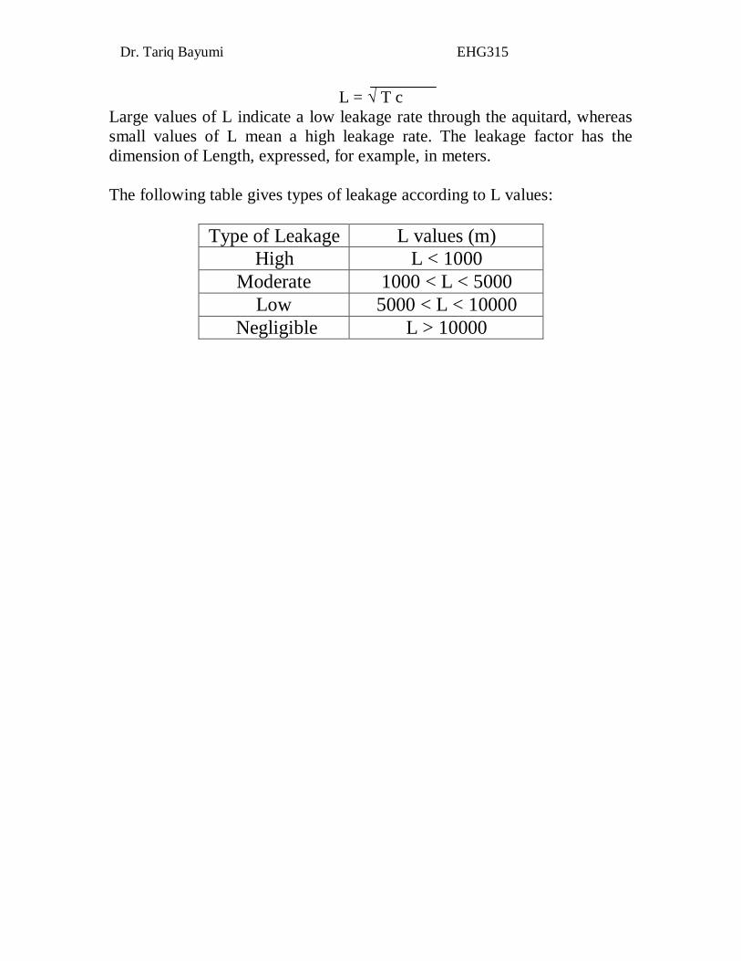
L = √ T c Large values of L indicate a low leakage rate through the aquitard, whereas small values of L mean a high leakage rate. The leakage factor has the dimension of Length, expressed, for example, in meters. The following table gives types of leakage according to L values:

L values (m) Type of Leakage L < 1000 High

1000 < L < 5000 Moderate 5000 < L < 10000 Low

L > 10000 Negligible




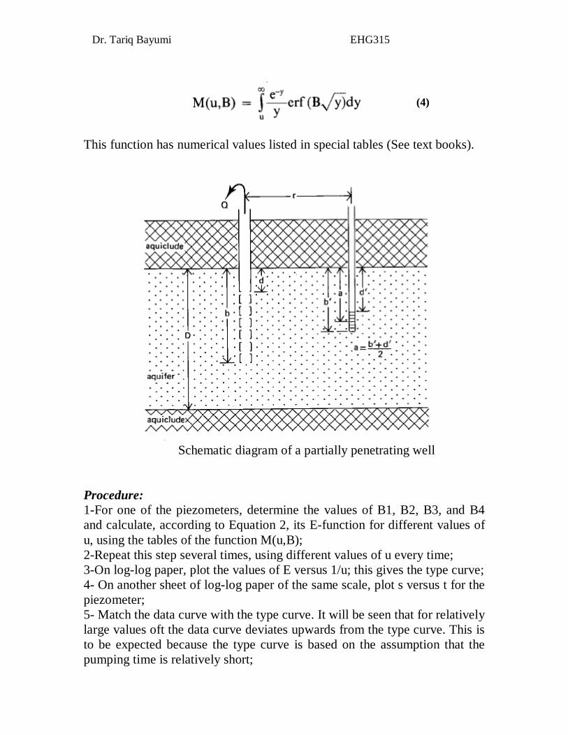
اآلبار ذات االختراق الجزئي Partially-Penetrating Wells

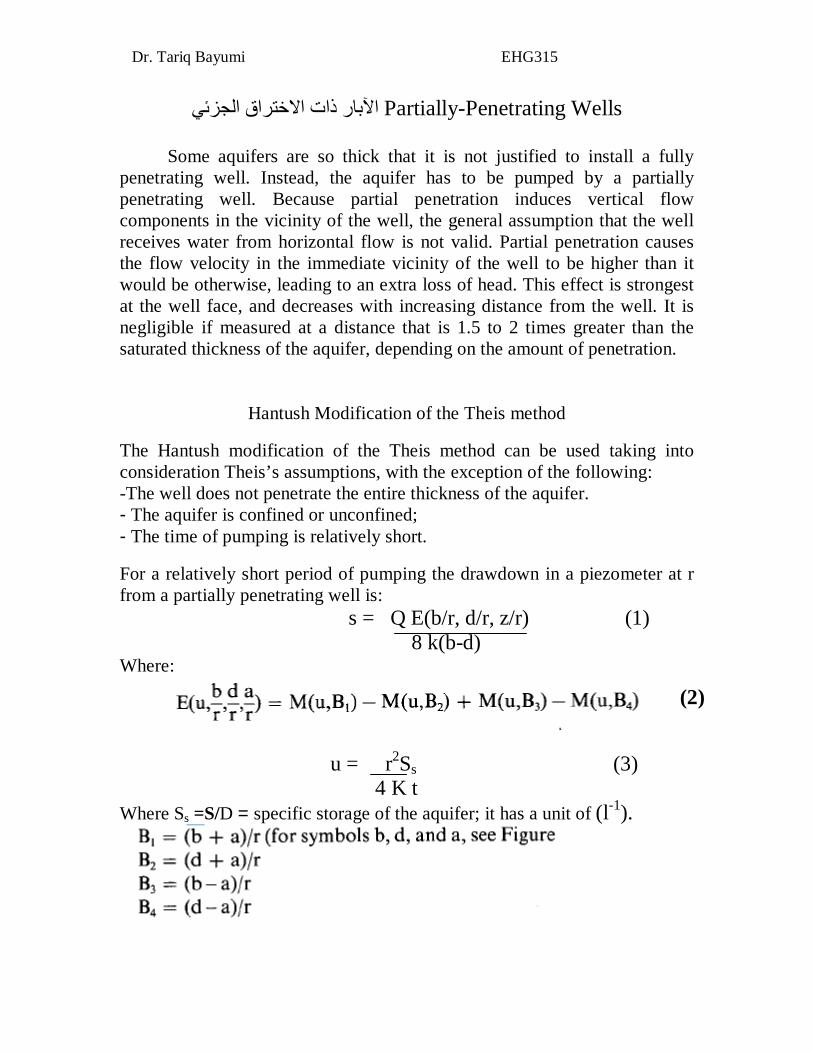
Some aquifers are so thick that it is not justified to install a fully penetrating well. Instead, the aquifer has to be pumped by a partially penetrating well. Because partial penetration induces vertical flow components in the vicinity of the well, the general assumption that the well receives water from horizontal flow is not valid. Partial penetration causes the flow velocity in the immediate vicinity of the well to be higher than it would be otherwise, leading to an extra loss of head. This effect is strongest at the well face, and decreases with increasing distance from the well. It is negligible if measured at a distance that is 1.5 to 2 times greater than the saturated thickness of the aquifer, depending on the amount of penetration.

Hantush Modification of the Theis method The Hantush modification of the Theis method can be used taking into consideration Theis’s assumptions, with the exception of the following: -The well does not penetrate the entire thickness of the aquifer. - The aquifer is confined or unconfined; - The time of pumping is relatively short. For a relatively short period of pumping the drawdown in a piezometer at r from a partially penetrating well is: s = Q E(b/r, d/r, z/r) (1)

8 k(b-d) Where:

u = r2Ss (3) 4 K t Where Ss =S/D = specific storage of the aquifer; it has a unit of (l-1).

(2)


This function has numerical values listed in special tables (See text books).

Schematic diagram of a partially penetrating well Procedure: 1-For one of the piezometers, determine the values of B1, B2, B3, and B4 and calculate, according to Equation 2, its E-function for different values of u, using the tables of the function M(u,B); 2-Repeat this step several times, using different values of u every time; 3-On log-log paper, plot the values of E versus 1/u; this gives the type curve; 4- On another sheet of log-log paper of the same scale, plot s versus t for the piezometer; 5- Match the data curve with the type curve. It will be seen that for relatively large values oft the data curve deviates upwards from the type curve. This is to be expected because the type curve is based on the assumption that the pumping time is relatively short;

(4)


6- Select a point A on the superimposed sheets in the range where the curves do not deviate, and note for A the values of s, E, l/u, and t; 7- Substitute the values of s and E into Equation 10.3 and, with Q, b, and d known, calculate K; 8- Substitute the values of I/u and t into Equation 1 and, with r and K known, calculate Ss; 9- If the data curve departs from the type curve, note the value of l/u at the point of departure, l/Udep; - Calculate D from the relation:

10- Calculate T and S using the relations:

T=KD, S=Ss D


رجوع (االستعاضة)اختبار ال Recovery Test

Recovery: The return of the water levels in wells after pump shut down to its original position prior to pumping. Residual drawdown : It is defined as the difference between the original water level before the start of pumping and the water level measured at a time t’ after the end of pumping. Recovery test Characteristics: -Recovery-test measurements allow the transmissivity of the aquifer to be calculated, thereby providing an independent check on the results of the pumping test, although costing very little in comparison with the pumping test, -Residual drawdown data are more reliable than pumping test data because recovery occurs at a constant rate, whereas a constant discharge during pumping is often difficult to achieve in the field, - Discharge value (Q) used in pumping test is also substituted in recovery test equation. - It is not possible to calculate S value using this method.

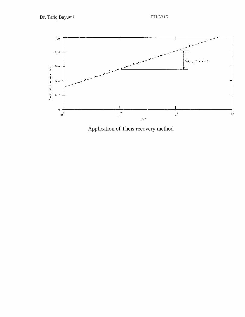
طریقة الرجوع لثایس Theis’s recovery method Procedure: 1- For each observed value of s‘, calculate the corresponding value of t/t’, where t’= time after pumping shut down and t= time since pumping started; 2- For one of the piezometers, plot s‘versus t/t’ on semi-log paper (t/t’ on the logarithmic scale) (see figure below); 3- Fit a straight line through the plotted points; 4- Determine the slope of the straight line, i.e. the residual drawdown difference Δs’ 5- Substitute the known values of Q and Δs‘ into the flowing equation and calculate T:

T = 2.3Q / 4π Δs’

Where Δs’= slope of straight line drawn between two consecutive log cycles.


Application of Theis recovery method


HYDROGEOLOGIC BOUNDARIES الحدود الهيدروجيولوجية

They are geological or hydrogeological formations that bound groundwater aquifer from one direction or more and influence the groundwater flow in the aquifer. They are divided into:

1- Barrier Boundary 2- Recharge Boundary 3- Multiple boundaries

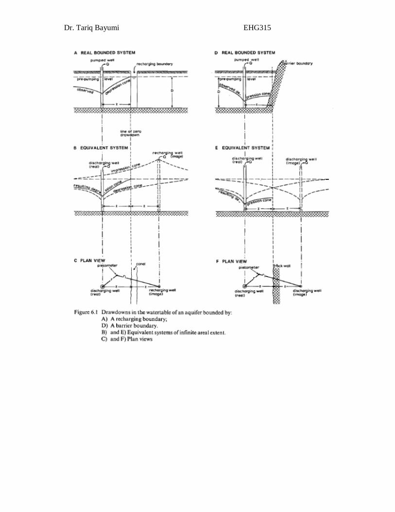
1- Barrier Boundaries These are geological impermeable formations that surround the

groundwater aquifer from one side or more and obstruct the movement of ground water from or into the aquifer. If we assume the existence of an impermeable barrier in the form of a straight line on one side of a confined aquifer, the drop in the piezometric surface due to pumping will be greater near the barrier compared to the one predicted by the Theis equation in the infinite aquifers (see Figure).

To predict the drop of groundwater level in such a system we use the METHOD of IMAGES. To achieve this, imagine a well drilled at a distance (x) behind the barrier which equals the distance between the real well and the barrier and discharging at the same rate (Q) and for the same period of time. As a result a cone of depression will form on the other side of the barrier in addition to the cone of depression formed by the real well. Therefore the two cones will intersect at the boundary, and the resultant cone of depression will be deeper near the boundary compared to that formed in the infinite extent conditions.

The drawdown in an aquifer bounded by a barrier boundary is: s = Q [W(u)r +W(u)i]

4 Л T Where: ur = rr

2 S / 4Tt ui = ri

2 S /4Tt rr= distance between real well and observation well; ri= distance between image well and observation well; t= time since pumping started.



2-Recharge Boundaries When an aquifer is surrounded from one side by a permanent recharge

boundary such as rivers and streams and the like, it is possible to estimate the drawdown in the groundwater level in a well drilled in this aquifer near the boundary of an assumed constant head using the method of images. If we imagine a river cutting through the entire thickness of an aquifer, the drawdown in a well fully penetrating this aquifer can be predicted if we imagine a well on the other side of the boundary. The image well recharges the aquifer at a constant rate Q equal to the constant discharge of the real well. Both the real well and the image well are located on a line normal to the boundary and are equidistant from the boundary. If we now sum the cone of depression from the real well and the cone of impression from the image well, we obtain an imaginary zero drawdown in the infinite system at the real constant-head boundary of the real bounded system. The water levels in wells drilled in the aquifers bounded by recharge boundaries drop in the beginning of pumping from the real well and when the effect of the image cone of the recharging well reaches the pumping well the rate of drawdown changes. The drawdown rate continues to drop until it reaches equilibrium state when the discharge equals the recharge. In this case we can calculate the drawdown using the following equation:

s = Q [W(ur)-W(ui)]

4 Л T

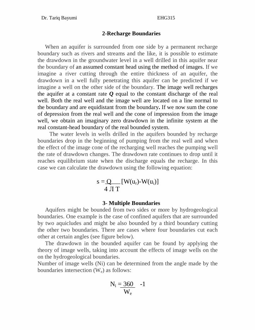
3- Multiple Boundaries Aquifers might be bounded from two sides or more by hydrogeological

boundaries. One example is the case of confined aquifers that are surrounded by two aquicludes and might be also bounded by a third boundary cutting the other two boundaries. There are cases where four boundaries cut each other at certain angles (see figure below).

The drawdown in the bounded aquifer can be found by applying the theory of image wells, taking into account the effects of image wells on the on the hydrogeological boundaries. Number of image wells (Ni) can be determined from the angle made by the boundaries intersection (We) as follows:

Ni = 360 -1

We


Times Law If we assume the existence of two observation wells at distances r1 and r2 from a well pump, the drawdown in those wells can be found by Jacob equation as follows:

s1=2.3Q log 2.25Tt1 4 Л T r1

2S

s2=2.3Q log 2.25Tt2 4 Л T r2

2S If we assume s1=s2,

log (2.25 Tt1) = log (2.25 Tt2) r2

2 S r12 S

i.e. t1/r1

2 = t2/r22


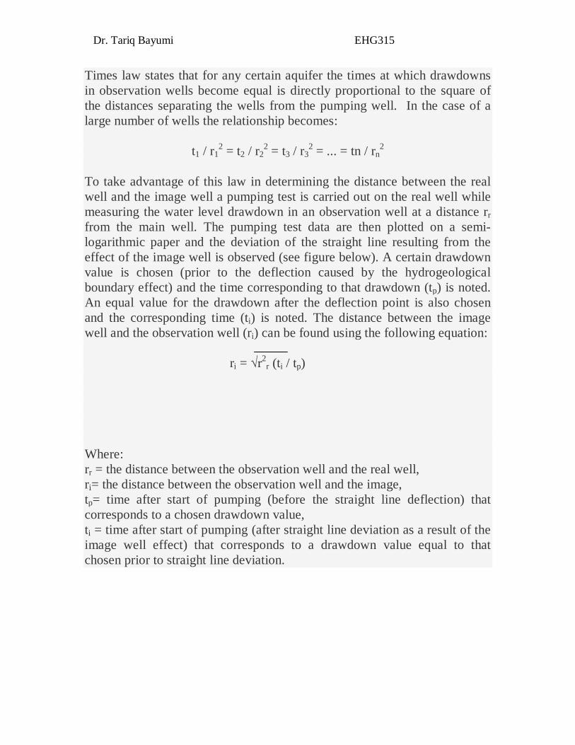
Times law states that for any certain aquifer the times at which drawdowns in observation wells become equal is directly proportional to the square of the distances separating the wells from the pumping well. In the case of a large number of wells the relationship becomes:

t1 / r1

2 = t2 / r22 = t3 / r3

2 = ... = tn / rn2

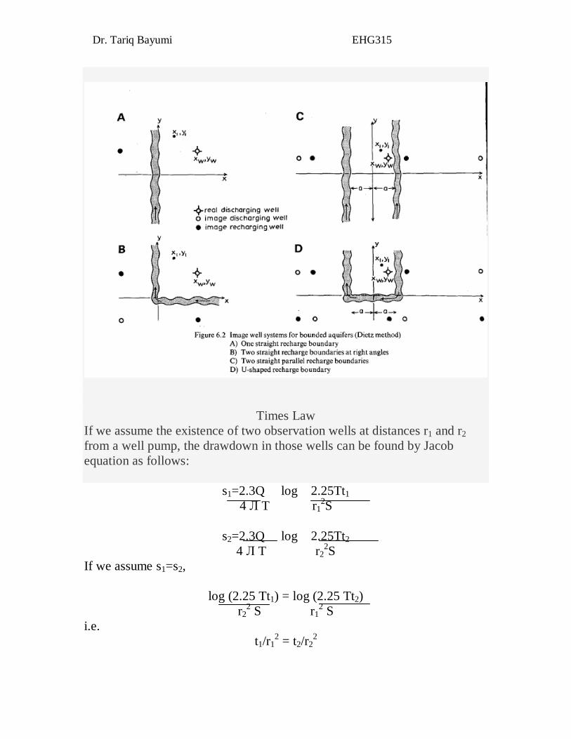
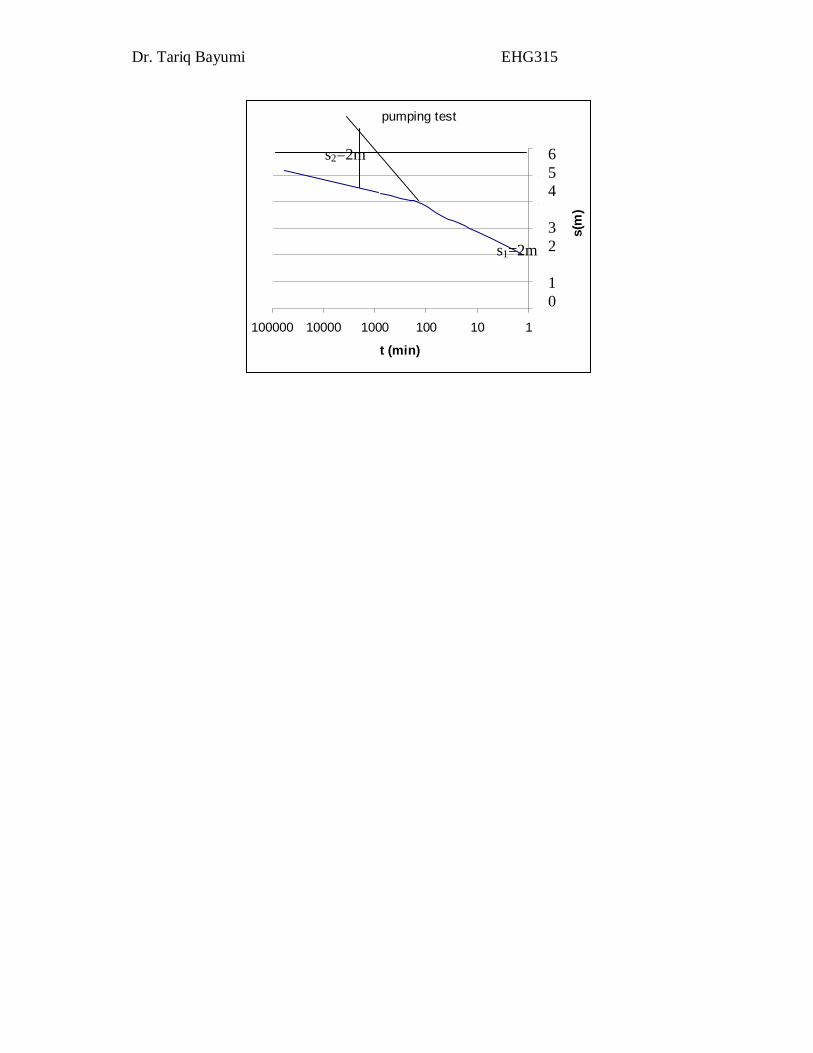
To take advantage of this law in determining the distance between the real well and the image well a pumping test is carried out on the real well while measuring the water level drawdown in an observation well at a distance rr from the main well. The pumping test data are then plotted on a semi-logarithmic paper and the deviation of the straight line resulting from the effect of the image well is observed (see figure below). A certain drawdown value is chosen (prior to the deflection caused by the hydrogeological boundary effect) and the time corresponding to that drawdown (tp) is noted. An equal value for the drawdown after the deflection point is also chosen and the corresponding time (ti) is noted. The distance between the image well and the observation well (ri) can be found using the following equation: ri = √r2

r (ti / tp) Where: rr = the distance between the observation well and the real well, ri= the distance between the observation well and the image, tp= time after start of pumping (before the straight line deflection) that corresponds to a chosen drawdown value, ti = time after start of pumping (after straight line deviation as a result of the image well effect) that corresponds to a drawdown value equal to that chosen prior to straight line deviation.


pumping test

2

2.5

3

3.5

4

4.5

5

110100100010000100000

t (min)

s(m

)

6 5 4 3 2 1 0

s1=2m

s2=2m


Multiple Well Systems and Interference اآلبار المتداخلة والتعدد

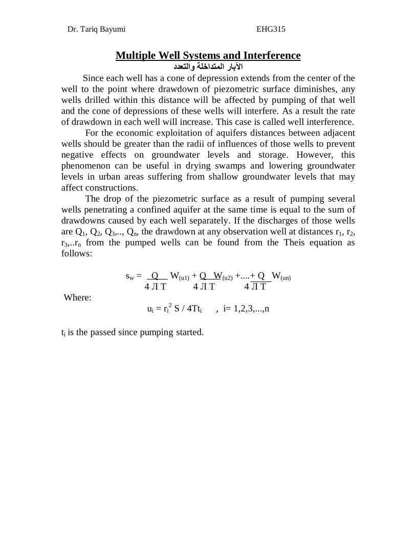
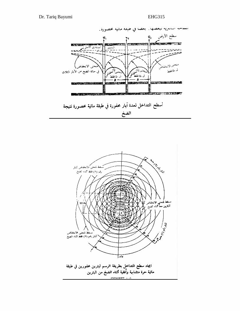
Since each well has a cone of depression extends from the center of the well to the point where drawdown of piezometric surface diminishes, any wells drilled within this distance will be affected by pumping of that well and the cone of depressions of these wells will interfere. As a result the rate of drawdown in each well will increase. This case is called well interference. For the economic exploitation of aquifers distances between adjacent wells should be greater than the radii of influences of those wells to prevent negative effects on groundwater levels and storage. However, this phenomenon can be useful in drying swamps and lowering groundwater levels in urban areas suffering from shallow groundwater levels that may affect constructions. The drop of the piezometric surface as a result of pumping several wells penetrating a confined aquifer at the same time is equal to the sum of drawdowns caused by each well separately. If the discharges of those wells are Q1, Q2, Q3,.., Qn, the drawdown at any observation well at distances r1, r2, r3,..rn from the pumped wells can be found from the Theis equation as follows:

sw = Q W(u1) + Q W(u2) +....+ Q W(un)

4 Л T 4 Л T 4 Л T Where:

ui = ri2 S / 4Tti , i= 1,2,3,...,n

ti is the passed since pumping started.


Documents

Groundwater Hydraulics EHG 315 Dr. Tariq Hassan Bayumi · Groundwater Hydraulics Introduction Groundwater hydraulics is a branch of the hydrogeological sciences that combines groundwater