Diplomarbeit

Hardware-based Timing

Synchronization

ausgefuhrt zum Zwecke der Erlangung des akademischen Grades

eines Diplom-Ingenieurs

unter der Leitung von

Univ.Prof. Dipl.-Ing. Dr.techn. Markus Rupp

Mag.rer.soc.oec. Dipl.-Ing. Dr.techn. Sebastian Caban

Institut fur Nachrichtentechnik und Hochfrequenztechnik

eingereicht an der Technischen Universitat Wien

Fakultat fur Elektrotechnik und Informationstechnik

von

Armin Dißlbacher-Fink

Oswald Spiegelfeld-Strasse 8

4840 Vocklabruck

Vocklabruck, Dezember 2010

Abstract

In 2005, the Institute of Communications and Radio-Frequency Engineering at

the Vienna University of Technology developed a rapid prototyping system to

characterize mobile communications algorithms under real world conditions. In

order to evaluate cellular radio communication systems, this system has been

recently extended to multiple transmitters and receivers. As a consequence of

this expansion, new hardware was required that is able to synchronize all base

stations and receivers in time. In this thesis, a distributed system has been

built which handles synchronous transmission and reception of data frames at

a predefined time instant. This synchronization system consists of standalone

devices with an internal clock locked to a reference clock signal generated

by a combination of a GPS receiver and a rubidium frequency standard. The

developed synchronization system is reliable and easy to integrate into existing

rapid prototyping systems as it only requires a (usually already existing) local

area network connection to operate. It supports a lot of different inputs and

outputs for precisely timing external hardware such as linear positioning tables.

Furthermore a software tool is provided that derives optimum system settings

depending on the given local area network environment it is operated in.

i

Kurzfassung

Am Institut fur Nachrichten- und Hochfrequenztechnik der Technischen Uni-

versitat Wien wurde 2005 ein rapid prototyping System aufgebaut, das es

ermoglicht Algorithmen, die fur Anwendungen der mobilen Kommunikation

entwickelt wurden, in einem realen Ubertragungssystem zu charakterisieren.

Um Mobilfunksysteme mit mehreren Zellen abbilden zu konnen muss das Sys-

tem auf mehrere Sender und Empfanger erweitert werden. Im Zuge dieser

Umstellung wird ein System benotigt, das die Synchronisierung aller Teilneh-

mer sicherstellt. Die in dieser Arbeit entwickelten Gerate ermoglichen dies und

somit das zeitgleiche Ubertragen und Empfangen eines Datenblocks zu einem

definierten Zeitpunkt. Zum Abgleich der Uhren der einzelnen Gerate wird ein

Referenztakt verwendet, der aus einer Kombination von GPS Empfanger und

Rubidium Frequenznormal erzeugt wird (diese Technik wird auch zur Syn-

chronisierung von Mobilfunk Basisstationen verwendet [1]). Das entwickelte

System zeichnet sich durch eine einfache Integrierbarkeit in das vorhandene

Umfeld, sowie eine hohe Zuverlassigkeit aus. Weiters wird ein Softwaretool zur

Verfugung gestellt, das die optimale Anpassung des Synchronisations Systems

an die Gegebenheiten des rapid prototyping Aufbaus ermoglicht.

ii

Contents

1 Introduction 1

2 Basic Idea 3

2.1 Initialization Procedure . . . . . . . . . . . . . . . . . . . . . . . 3

2.2 Timestamp Based Triggering . . . . . . . . . . . . . . . . . . . . 4

2.3 Communication Network . . . . . . . . . . . . . . . . . . . . . . 5

2.4 Information Flow . . . . . . . . . . . . . . . . . . . . . . . . . . 6

2.4.1 Initial Startup . . . . . . . . . . . . . . . . . . . . . . . . 6

2.4.2 Announce Process Duration . . . . . . . . . . . . . . . . 7

2.4.3 Restore after Error . . . . . . . . . . . . . . . . . . . . . 8

2.5 Reference Signals . . . . . . . . . . . . . . . . . . . . . . . . . . 8

2.5.1 Clock Signal . . . . . . . . . . . . . . . . . . . . . . . . . 8

2.5.2 Synchronization Signal . . . . . . . . . . . . . . . . . . . 9

3 Timing Unit 10

3.1 Real-Time Part . . . . . . . . . . . . . . . . . . . . . . . . . . . 12

3.1.1 Input Clock . . . . . . . . . . . . . . . . . . . . . . . . . 12

3.1.2 1PPS Signal . . . . . . . . . . . . . . . . . . . . . . . . . 13

3.1.3 Reset Logic . . . . . . . . . . . . . . . . . . . . . . . . . 13

3.1.4 48 Bit Counter . . . . . . . . . . . . . . . . . . . . . . . 14

3.1.5 Compare Unit . . . . . . . . . . . . . . . . . . . . . . . . 14

3.1.6 Trigger Output . . . . . . . . . . . . . . . . . . . . . . . 14

3.1.7 System Extension Interfaces . . . . . . . . . . . . . . . . 14

3.2 Communication Part . . . . . . . . . . . . . . . . . . . . . . . . 15

3.2.1 Software Architecture . . . . . . . . . . . . . . . . . . . . 18

3.2.2 Control Commands . . . . . . . . . . . . . . . . . . . . . 18

3.2.3 UART Commands . . . . . . . . . . . . . . . . . . . . . 22

3.3 Controlling the Timing Unit via Matlab . . . . . . . . . . . . . 25

3.3.1 Open Port . . . . . . . . . . . . . . . . . . . . . . . . . . 26

3.3.2 Send Packet . . . . . . . . . . . . . . . . . . . . . . . . . 26

iii

3.3.3 Receive Packet . . . . . . . . . . . . . . . . . . . . . . . 27

3.3.4 Close Port . . . . . . . . . . . . . . . . . . . . . . . . . . 28

4 Performance Analysis 29

4.1 Timing Unit Characteristics . . . . . . . . . . . . . . . . . . . . 29

4.1.1 Trigger Signal . . . . . . . . . . . . . . . . . . . . . . . . 29

4.1.2 Jitter Analysis . . . . . . . . . . . . . . . . . . . . . . . 29

4.2 Link Characterization . . . . . . . . . . . . . . . . . . . . . . . . 32

4.2.1 Packet Loss Rate . . . . . . . . . . . . . . . . . . . . . . 33

4.2.2 Packet Delay Profile . . . . . . . . . . . . . . . . . . . . 34

4.2.3 Trigger Process Duration . . . . . . . . . . . . . . . . . . 35

4.2.4 Optimum Trigger Time . . . . . . . . . . . . . . . . . . . 38

4.3 Link Timing Comparison . . . . . . . . . . . . . . . . . . . . . . 39

4.3.1 Optical Fiber Connection . . . . . . . . . . . . . . . . . 41

4.3.2 Directive Radio Link . . . . . . . . . . . . . . . . . . . . 41

4.3.3 Low-Cost WLAN Connection . . . . . . . . . . . . . . . 42

4.4 Discussion of the Results . . . . . . . . . . . . . . . . . . . . . . 43

5 Conclusion 44

Bibliography 45

iv

1. Introduction

1 Introduction

This thesis treats a synchronization problem that occurs at a test system for

algorithms in mobile communication. The system consists of a wireless trans-

mitter, which is basically a personal computer with a digital to analog converter

board, and a wireless receiver, which is also PC based but in contrast to the

transmitter uses an analog to digital converter board. Both sides are controlled

by a Matlab1 script, which in the case of the transmitter, writes data samples

to the converter board. At the receiving side, the Matlab script then copies

the received samples from the converter board to hard disk.

Both PCs are located at different floors of an office building or could even

be located at different buildings. Now the problem arises, that even if both

converter boards are located far away from each other, they have to be started

at the same time in order to perform a wireless data transmission between the

PCs (Figure 2.1).

This thesis describes a system, that is able to synchronize two or more converter

boards by the help of a LAN2 connection and a common timing reference

delivered by a GPS3 receiver (Figure 1.1).

Chapter 2 of this thesis introduces the basic idea for solving the synchronization

problem. A general structure as well as the principle of operation is discussed.

Furthermore, all protocols and interfaces are defined.

1 Matlab is a product of The MathWorks Inc.2 LAN - Local Area Network3 GPS - Global Positioning System

1

1. Introduction

Matlabtiming

unitGPS

1PPS

CLK

TRIG

FIFOTX card

transmitter

Matlabtiming

unitGPS

TRIG

FIFORX card

receiver

common

reference

LAN

1PPS

CLK

Figure 1.1: On every site of the test system, the timing unit is responsible for syn-chronization of the transmission/reception

The first part of Chapter 3 addresses the developed hardware. Issues like

real time capability are discussed and a flexible platform for implementing the

synchronization system is presented. The second part of this chapter covers

the software structure of the developed boards. Furthermore, a set of Matlab

functions for controlling the system is introduced.

In Chapter 4, the performance of the system is analyzed and optimized with

respect to maximum data rate between transmitter and receiver.

2

2. Basic Idea

2 Basic Idea

The timing synchronization system to be developed has to operate in an al-

ready existing environment. Therefore, parts of the given infrastructure are

reused. The timing system is designed as a set of standalone units where ev-

ery unit handles synchronization of one site of the test system. Therefore the

number of units has to match the number of sites.

The basic idea to achieve synchronization is to acquire the current time via the

help of a GPS receiver. Furthermore, a local area network connection among

all sites is used to spread timestamps at which a data transmission has to be

started.

2.1 Initialization Procedure

Before the first trigger process can be started, the system has to synchronize

the internal clocks of all timing units. The synchronization procedure is started

by an UDP command to one involved unit. This unit waits for the next 1PPS 1

pulse and then tells all other units to start their local clocks at the next 1PPS

event. The other units receive this command and at the next 1PPS pulse

all clock counters start synchronous. This process only performs properly, if

the message, to start the clock at the next 1PPS event, arrives at every node

within one second.

1 1PPS - one pulse per second

3

2. Basic Idea

2.2 Timestamp Based Triggering

After successfully synchronizing, all units know the same relative time and

timestamp based triggering can be carried out. To start a trigger process,

the controlling Matlab program of one site has to tell the timing unit, located

at the same site, the time when the next conversion can be started. This

information has to be stated as a relative time difference, because the PC has

no knowledge of the precise actual time. One possible message to the timing

unit would be: ”start all converter boards in 5 ms”. The timing unit then looks

up the actual time and adds 5 ms. This results in a timestamp, that is spread

over the network to all other timing units which then trigger at the same time

their connected converter boards.

From this procedure it can be seen that a ”start conversion in 0 ms” has to

result in an error due to the network delay that the timestamp message expe-

riences. Consequently, the Matlab program has to include the network delay

into its time announcement. A method for determining an optimum value

representing the network delay, is supplied in Chapter 4.

signal generation

signal generation

signal transmission

signal transmission

signal reception signal analysis

time

time

time

transmitter 1

transmitter 2

receiver 1

trigger

trigger

trigger

Figure 2.1: Timing example with two transmitters: both transmitters and thereceiver have to be triggered at the same time to perform a datatransmission.

If the scenario is extended to two transmitters, then two timestamps for trig-

gering are spread over the network. Obviously the data transmission is only

successful, if the converter boards are started at the latest of these two in-

stances. In the other case, one of the sites is not ready to perform its destined

action. The same argument applies after extending the system to an arbitrary

number of participants. This multi user scenario can be implemented in the

timing units by simply comparing all timestamps and triggering at the largest

4

2. Basic Idea

one. This can only be done if every timing unit knows the number of incom-

ing time stamps to wait for. Therefore the number of units in the setup is

announced in the initialization phase.

The principle of trigger time announcement is not restricted to transmitting

sites only. On the receiving side, the Matlab script may need some time

to readout data from the previous transmission and it is therefore necessary

to delay the next transmission. This can be done by announcing a trigger

time, larger than the duration after which the receiving hardware is ready for

operation. Throughout the remainder of this thesis, sites which influence the

trigger process, by announcing trigger durations are called active. If a site

does not influence the trigger timing (not trigger time announcements), it is

called passive.

2.3 Communication Network

Ethernet was chosen as the communication network between the timing units.

This is convenient because the interfacing to the timing system can be done

via the same communication system as the signaling. Furthermore, Ethernet

is a standard technology that is available almost at every office. Another

advantage is the ability to interconnect different sites via the Internet, which

enables large distances between different sites. As communication protocol,

UDP2 is used. UDP has the ability to send broadcast messages which allows

to reach all other timing units by sending only one data packet. Because of

the limited resources of the timing units, this speeds up communication and

therefore enhances the system performance. The drawback, on the other hand,

is the missing error handling. Therefore, it is not guaranteed that a packet

arrives at its destination. Due to these facts some kind of error handling has

to be implemented. To allow for maximum flexibility of the system, the whole

error handling has to be done by the controlling software (Matlab script of one

site). Only few errors are reported by the timing system and the leftovers have

to be caught by appropriate timeouts. Note that the messaging is designed in

such a way that if a successful transmission is reported, the transmission has

been successful. In case this report is missing, the transmission is considered

non successful, even if this is not necessarily the case.

2 UDP - User Datagram Protocol

5

2. Basic Idea

2.4 Information Flow

The subsequent part constitutes the information flow, initiated by the available

system commands. A detailed discussion of the commands is provided in

Section 3.2.2.

2.4.1 Initial Startup

initialize

1PPS1PPS

1PPS1PPS sync.

init. Ok

Matlab 1

networkdelay

resetclock counters

sync. Ok

time

timing

unit 1timing

unit n

Figure 2.2: Initialization of the timing system

To initialize the timing system, one Matlab script has to send a command,

including the number of active and passive sites, to the timing unit located

at the same site. It does not matter which site starts the initialization be-

cause this phase affects the whole timing system. The topology information,

included in the initialize command, is spread over the timing network and the

clock counters of the system are synchronized. As a reaction to successfully

synchronizing, an ”init ok” message is sent to the initializing host. Figure 2.2

shows the information flow on setting up the timing system. Due to the net-

work delay of the link, the messages need time to travel between the units.

This delay can also be seen in Figure 2.2. The synchronization procedure

6

2. Basic Idea

is started at a 1PPS event. More details about reference signals and their

synchronization can be found in Section 2.5.

If one, or more packets are lost in the initialization phase, the ”init ok” com-

mand does never arrive. Therefore an error handling procedure has to be

implemented in the initializing host.

2.4.2 Announce Process Duration

At every active site, the Matlab script has to tell the timing system the first

possible time, when the conversion process can be triggered. Therefore, the

command is named ”trigger in x”, where x is the time difference from the

actual time to the moment the conversion can be started.

trigger in x

y = current timestamp

trigger at x+ y

trigger Ok

x

trigger Ok

. . . trigger pulse

time

Matlab 1timing

unit 1timing

unit n

Figure 2.3: Announce duration and trigger

If the trigger time is chosen without regard to the network delay, it can happen

that one member of the timing system is not able to trigger at the right time

instant. After such an event occurred, all other timing units are informed and

they pass the information to their assigned Matlab scripts. As a supporting

information, the largest time difference is reported (see ∆t in Figure 2.4).

7

2. Basic Idea

trigger in x

y = current timestamp

trigger at x+ y

trigger error ( t)

x

trigger error ( t)

. . . trigger pulse

ttime

Matlab 1timingunit 1

timingunit n

Δ Δ

Figure 2.4: Trigger error due to network delay

2.4.3 Restore after Error

In case of an error, due to lost packets or too early trigger time instances, the

system has to be reset to a defined state. This has to be done after every

trigger error and can be started by a Matlab script by sending an ”abort”

command to its assigned unit (Figure 2.5). The command is then passed to

all members of the timing system which restore their internal registers. After

a successful restore, the timing system answers with a ”ready for commands”

message and the next trigger time can be set.

2.5 Reference Signals

To allow for appropriate synchronization of all sites, the timing system needs

two supporting reference signals.

2.5.1 Clock Signal

A clock signal has to be supplied to the converter boards, which is synchronous

to the clock signals at all other sites. This can be ensured by feeding all

devices with a clock generated via one common oscillator and distributing

this clock via coaxial cables. Unfortunately, this approach is restricted to

short distances between sites, especially to sites located in the same building.

Another possibility, which is used for the transmission system discussed in

Chapter 1, is to lock a local oscillator to the reference signal of a GPS satellite.

8

2. Basic Idea

abortmeasurement

abort

ready forcommands

abort done

time

Matlab 1timing

unit 1

timing

unit n

Figure 2.5: Restore after error

2.5.2 Synchronization Signal

Figure 2.2 shows that the internal clocks of the timing units are reset at an

event, that is denoted as 1PPS. This signal has to be available at all sites

to ensure synchronization of all units. The minimum demand on this signal is

to supply at least two pulses, separated by a duration longer than the largest

single trip time in the employed network. Also the phase relation to the clock

signal has to be fixed. Like the clock signal, the 1PPS signal also can be

supplied by cables connected to one reference. But for long distances and GPS

synchronized clocks, the 1PPS signal can also be locked to a satellite.

9

3. Timing Unit

3 Timing Unit

Figure 3.1: Timing unit

This chapter shows the design of a timing unit that is appropriate to the

definition of the previous chapter. All relevant data, like schematics, layout,

source code and files for the casing are stored on a CD enclosed to this thesis.

The design was done with respect to maximum flexibility. Therefore the system

can be further enhanced or adapted to lots of different timing applications

without changing the hardware.

The developed timing unit is a standalone device. It consists of a main board

which carries all the active components and a front panel for status LEDs and

an optional JTAG1 debugger. Figure 3.1 shows the front view of a timing unit.

The design of the main board can be split up into three parts:

1 JTAG - Joint Test Action Group

10

3. Timing Unit

trig

ger

out

cloc

k in

1PP

S in

8x r

elay

out

LA

N

6V

6x d

igital

I/O

4x o

pto

in

3x s

ignal

out

COM0-2

frontpanel

8x digital I/O

rese

t

2x b

utt

on

Figure 3.2: Main board

Power supply: The power supply is located on the right side of the main board

(Figure 3.2). It converts the 6 V input voltage to 3.3 V, 1.8 V and 3.5−5.0 V.

Communication Part: The components for this part are located next to the

power supply and consist of a microcontroller and a LAN interface. This

part handles the communication among all timing units, as well as to the

Matlab script and the real time part of the board.

Real Time Part: This part occupies the largest area of the main board. The

main parts are a CPLD 2 (see largest chip on Figure 3.2) and a clock divider

chip. It is called real time, because all functions are directly implemented

in hardware, which results in a deterministic and fast system. Due to the

CPLD, all logical functions can be changed to the requirements of the spe-

cific environment by firmware updates.

2 CPLD - Complex Programmable Logic Device

11

3. Timing Unit

LAN clock divider + delay

CPLD

application

IP Stack

32-bit ARM CPU

trigger

reset

timing unit

/8

compare unit

48-bit

shift register

48-bit

counter

reset / sync.

logic

Δt

signals to trigger - target

/1

/2

/3

/4

clock

1PPS

Figure 3.3: Timing unit - schematic

3.1 Real-Time Part

The real time part mainly consists of a CPLD that is controlled by a micro-

controller. The reason for choosing a CPLD is that due to precision problems,

the required counter and compare unit cannot be implemented by software in

a microcontroller. With a CPLD it is possible to build a custom chip with

all required features by defining the hardware in VHDL3. Furthermore it is

possible to reconfigure the system by simply reprogramming the CPLD. For

example, instead of connecting external devices directly to the microcontroller,

all lines are routed through the CPLD. This enables rewiring nearly every part

without the need for soldering on the main board. With this method, the sys-

tem is very flexible and is therefore well suited for rapid prototyping systems.

In the following, all components of Figure 3.3 are discussed in detail.

3.1.1 Input Clock

The input clock to the timing unit has to be locked to the clock of the target

in order to trigger. The maximum level of the signal is 1.2 Vpp. Internally, the

CPLD is able to handle clock frequencies up to a maximum of 100 MHz. To

be able to use higher clock frequencies for the trigger target, a clock divider is

installed between the clock connector and the chip. This divider can be set to

3 VHDL - Very High Speed Integrated Circuit Hardware Description Language

12

3. Timing Unit

four different values (divide by: 1, 2, 3, 4) and therefore allows for a maximum

input frequency of 400 MHz. Furthermore, the clock signal to the CPLD can be

delayed in four steps to align the generated trigger pulse roughly between two

rising edges of the clock. This is useful because most target boards will start

working when the trigger input is high and a rising edge of the clock signal

occurs. With this method also a very large jitter of the generated trigger pulse

in the range of about a quarter of the clock period does not influence the

accuracy of the system. Therefore, it can be guaranteed that all conversion

processes are started at the same rising edge (only valid for division factor of

one).

This clock divider can not be reset at the initialization phase and therefore at

division factors larger than one, the output signal can have a different phase

compared to the other timing units. It depends on the application, if this can

be tolerated or not. In the case of a wireless transmission system, a phase shift

of the trigger signal corresponds to a virtual change in antenna distance and

since the offset is constant, this offset does not change until the next system

initialization. Furthermore, the reference clock signals of different sites are

synchronized via a GPS satellite. The jitter among the clock signals is in the

range of about four clock cycles whereas the maximum phase shift corresponds

to three clock cycles.

The divided clock is fed to the CPLD where it is again divided. This sec-

ond clock divider has the ability to be reseted at the initialization phase syn-

chronous to the 1PPS signal and, therefore, no uncertainty in phase is added.

3.1.2 1PPS Signal

The 1PPS signal is only used at the initialization phase of the system, to

reset the internal clock divider and the clock counter. Therefore, this signal

directly affects the precision of the trigger output. The 1PPS signals of different

stations have also to be locked to the same common reference. This signal has

to be supplied to the timing unit as 2.5 Vpp@50Ω pulse. As discussed in the

previous chapter, this signal can be deactivated after the initialization phase.

3.1.3 Reset Logic

The reset module inside the CPLD is activated by the microcontroller and then

resets the clock counter and clock divider synchronously to the next rising edge

13

3. Timing Unit

of the 1PPS signal.

3.1.4 48 Bit Counter

The counter starts working after successfully synchronizing the timing system.

Depending on the input clock and the setting of the divider chip, the duration

until a counter overflow occurs can vary from a few days to several weeks.

Within this time, the timestamps are uniquely defined. After an overflow

occurred, the timer again starts at zero. A counter overflow does not influence

the precision of the timing system, because it occurs at the same time at all

timing units.

3.1.5 Compare Unit

The compare unit consists of a 48 bit shift register, which is loaded with times-

tamps by the microcontroller. The content of the clock counter is continuously

compared to this register. This results in the fact that for loading new times-

tamps the compare match output has to be deactivated. Therefore, for a

successful trigger process, the next time stamp has not to be loaded before the

actual trigger occurred. In this implementation the trigger granularity is set

to 0.04096 ms (213· 1/(200 MHz)).

3.1.6 Trigger Output

The trigger output is currently set to generate a pulse. Another option is to

set the trigger output to toggle mode, which is useful for watching the signal

on an oscilloscope. On the front panel of the timing unit there are three SMA

connectors, which can also be used as trigger outputs. A further option for

the trigger is to generate a pulse, when the timing unit receives a ping request.

This option is also useful for system testing and can be activated by setting a

specific flag via the UDP interface of the timing unit.

3.1.7 System Extension Interfaces

Additional interfaces are available at the timing unit to enable the integration

of external devices into the timing system. In the current design, the extension

interfaces are remote controlled via UDP commands.

14

3. Timing Unit

Trigger on external signals: The system has the ability to generate a trigger

pulse after waiting for an external signal. In detail, this means that the

user can send a ”trigger in x” command to its assigned unit, where x is

the duration between the occurrence of the external signal and the trigger

pulse. This works under the condition that the duration x is larger than the

maximum single trip time between all timing units on the network used.

Outputs: Every timing unit has 22 outputs, eight of them are relay outputs,

the rest is directly connected to the CPLD and could also be used as inputs

(requires changes in the VHDL code of the CPLD). Currently all outputs

can be remote controlled by UDP commands.

Inputs: To connect external devices, or react to external signals, the timing

unit has four opto-coupled inputs. This inputs are designed for 12 V signals.

By changing one resistor per input, they can be configured for different input

voltages. Furthermore two switches are located at the front panel, which

are currently not used.

RS232 interfaces: Another option to interface external devices via the tim-

ing unit is via RS232. There are three of these serial ports available per

timing unit. Only RX and TX lines are available on the connectors, addi-

tionally, COM0 has the option to interconnect the handshake lines. In the

current configuration, the serial ports can be controlled by any PC via UDP

commands.

CAN interface: For further projects, a CAN4 interface was added as an option

to the timing unit. COM3 is a shared connector, which can be either used

as RS232 interface, or as CAN interface. To make use of the CAN bus, the

software for the microcontroller has to be implemented and the CAN line

driver chip has to be assembled at the bottom side of the main board.

3.2 Communication Part

This part of the timing unit consists of a 32-bit microcontroller that interfaces

the CPLD and handles communication via Ethernet. The microcontroller

including the network interface is compatible to the MCB2360 [2] board from

KEIL. Therefore, software tests can also be performed by using this evaluation

board. Every timing unit is assigned to one site by its IP address. A timing

4 CAN - Controller Area Network

15

3. Timing Unit

unit always has an address 10.0.0.x1, where x denotes the number of the site.

The Matlab script, on the other hand, is running on a PC which always uses

10.0.0.x0 as IP address, x again denotes the number of the station. A timing

unit only executes trigger commands sent by a host with a corresponding

IP address (on the correct port and from the correct port). Communication

among the timing units is carried out via subnet broadcasts. To distinguish

different connections, the timing system uses several ports. One pair of ports

is used to exchange control and status information between the assigned PC

and the timing unit. This connection is only used to send commands related to

the trigger process. Another port is used by the timing units to communicate

among them. Here the packets are broadcasted and therefore all participating

units use the same port number. Via this connection, trigger timestamps are

spread between the units and also success or error messages are transmitted.

A third broadcast port is used to control the relay outputs and the serial ports

of the units (Figure 3.5 and Table 3.1).

d

b

ac

dc

a

b

dc

dc

Timing Unit10.0.0.21

1:1 connectionfor trigger commands

Timing Unit10.0.0.31

Timing Unit10.0.0.41

Timing Unit10.0.0.11

1:nconnection

1:n c

onnec

tion

for

UA

RT

and r

elay

com

man

ds

Matlab program 10.0.0.10

Matlab program10.0.0.20

1:1

connec

tion

for

trig

ger

com

man

ds

Figure 3.4: Example for IP and port assignment

16

3. Timing Unit

FLAGS

system initialization

check for received

UDP packet

set flags depending on

received command

state-machine 1

(handle actions)

state-machine n

(handle actions)

check for received

UDP packet

check for UDP

packet to send

send packet

depending on flags

Figure 3.5: Microcontroller software

port number description

a 13571b 13570

control commands and response

c 13581d 13580

UART commands and response

e 13550 communication among timing units

Table 3.1: UDP ports used for communication (see also Figure 3.4)

17

3. Timing Unit

3.2.1 Software Architecture

The basis for the software in the microcontroller is the application note

AN10799 from NXP [3], which handles ICMP messages, ARP requests and

stores received UDP packets in a receive buffer. After system startup, the

user application continuously checks for received packets. If a command was

received, the specific flags are set, which influence the behavior of the state

machines (see Figure 3.5). The idea behind this structure is that the result-

ing system is non-blocking and several tasks can be handled in parallel by

different state machines. For example, one state machine waits for data on a

UART port and after a given timeout sends the received bytes to a PC. In

parallel, a second state-machine handles communication to the timing system

in order to prepare for the next trigger process. The system can be extended

by adding another state machine, that is controlled by additional flags, which

can be set via UDP commands. Also coupling of different state machines, or

synchronizing tasks by using common flags, can be realized.

3.2.2 Control Commands

The timing unit listens on port 13570 for UDP packets. Only packets from the

assigned IP and originator port 13571 are accepted. Commands are strings,

encapsulated in a UDP packet. Available commands for the timing system are

listed below:

Start Initialization Procedure

This command starts synchronization of the internal clock counters to the

1PPS signal. The parameters specify, how many active sites and passive sites

have to be synchronized (the sum of both has to match the number of connected

timing units). The maximum number of timing units is currently limited to

26, this is due to the selection of the IP address assignment (timing unit 0. . . 25

correspond to IP address x.x.x.1. . . x.x.x.251). By choosing an other address

structure, the number of units can be extended.

18

3. Timing Unit

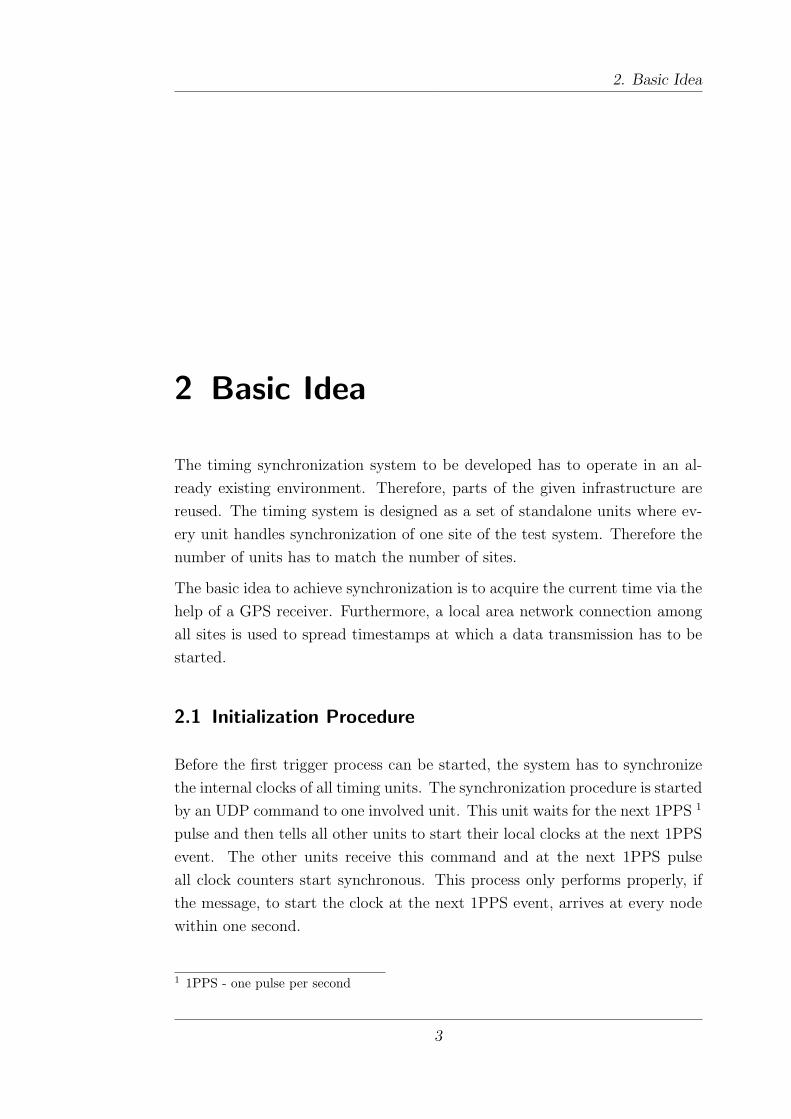
command: start <active devices>,<passive devices>

parameters: char active devicesnumber of active timing units in current environ-

ment

char passive devices

number of passive timing units in current environ-

ment

answer: all units in sync\n

Announce Process Duration

With this command, the Matlab script tells the timing system when it will

have finished and the conversion process can be started. Also the values for

the output ports are included.

19

3. Timing Unit

command: trigger <relays><IO ext><IO int> <trigger in>

parameters: uint8 relays

defines the state of the relay outputs of the timing

unit. Every bit represents one output.

uint8 IO extcontrols the 3.3 V outputs on the front panel of

the timing unit. Every bit, except the highest two,

represents one output (there are only 6 outputs on

the front panel).

uint8 IO intcontrols the 3.3 V outputs available at the pin

header inside the timing unit. Every bit represents

one output.

string trigger in

the trigger time stamp is generated as the sum

of the timestamp when this message arrived at

the timing unit and the trigger in value; has to

be exactly nine characters long. For example

”000000010” means, that the synchronous pro-

cess can be started in 10 clock counter ticks(=

0.4096 ms). If only the outputs should be changed,

than ” NaN” has to be sent as the trigger

time.

answer: success!\nif all converter boards were started correct

string <time difference >

in case of an error, the system reports the largest

time difference of announced trigger time and pos-

sible start time of the synchronous process. For ex-

ample, −52 means that one unit missed the trigger

by 52 counter ticks.

outputs ok\nif only outputs had to be changed.

20

3. Timing Unit

Set Flags

This command enables or disables specific functions of the timing unit during

run time.

command: flags <flag1><flag2><flag3>

parameters: char flag1

trigger on external signal: For values different to

”0,” the conversion process is started with respect

to an external signal (see Section 3.1.7, part trigger

on external signals).

char flag2

return timestamp on ping: For values different to

”0,” the timing unit reads out the actual time-

stamp when a ping request arrives and returns the

information via a UDP message to the assigned IP

address. This feature can be used to determine

single trip times in a network.

char flag3

trigger on ping: For values different to ”0” the

timing unit outputs a trigger pulse at the reception

of a ping request. Note that only the timing unit

that received the ping outputs the pulse and not

all units.

answer: flags ok\n

Abort Current Measurement

If the last trigger process was not successful, or the success message did not

arrive, the timing system has to be reset to a defined state. The abort mea-

surement command has to be sent to one timing unit and is then spread over

the network. The system answers with an abort done message and the next

trigger process can be started.

command: abort measurement

parameters: none

answer: abort done\n

21

3. Timing Unit

Reboot Timing Unit

Reboots the timing unit. Clock counter synchronization and all settings are

lost after this command.

command: reboot

parameters: none

answer: ready for commands\n

Reset the Real Time Part

Resets the CPLD to its initial state. Clock counter synchronization is lost

after this command, therefore the whole timing system has to be initialized

again before the next trigger process can be started. This does not reset the

microcontroller flags.

command: reset

parameters: none

answer: reset done\n

Beep

Activates the system beeper inside the unit for a duration of 0.5 sec.

command: beep

parameters: none

answer: beep ok\n

3.2.3 UART Commands

Three UART ports are available per timing unit, which can be remote con-

trolled via UDP messages. In contrast to the control commands, which are

directly addressed to one unit, the UART commands are sent as broadcasts.

This enables multiple devices to react to the same UDP message and allows

to trace communication between devices with a standard packet sniffer. Every

timing unit listens on port 13580 for incoming UART commands, that were

sent from port 13581. The available commands are listed below:

22

3. Timing Unit

Set UART Baud Rate

It is possible to change the baud rate of all UART ports dynamically via UDP

commands. Due to internal clock prescaler settings of the microcontroller,

the range of baud rates is limited. Currently only rates up to 57600 baud

are supported, if higher baud rates are required, then the clock system of the

microcontroller has to be reconfigured.

command: set <device number> <uart number> <baud rate>

parameters: char device numberspecifies which timing unit has to react to the

packet

char uart number

number of UART port to change baud rate (0. . . 2)

string baud rate

must be of length five and defines baud rate for

chosen port

answer: baud rate changed\n

Print Data to UART Port

This command sends data to external devices, which are connected to a UART

port. For the sake of generality, the data to be sent has to be supplied as a

byte array.

23

3. Timing Unit

command: print <device number> <uart number> . . .

. . . <ack before transmit> <ack after transmit> . . .

. . . <length> <data>

parameters: char device numberspecifies which timing unit has to react to the

packet

char uart number

number of UART port to output data (0. . . 2)

char ack before transmit

if 6= ”0” answer message is sent before transmitting

UART data.

char ack after transmit

if 6= ”0” answer message is sent directly after

last byte has been written to the UART transmit

buffer, that is, right before the last byte is trans-

mitted.

string length

must be of length two (a maximum of 99 bytes can

be transmitted via one UDP command), specifies

the number of bytes to send

byte array data

data to send via UART

answer: print <device number> <uart number> ok\noccurs twice if both ack flags are 6= ”0”

none

if both ack flags are equal to zero

Read Data from UART Port

Data that is sent from external devices to the timing unit’s UART port is

written to an internal buffer of length 99 (same length as transmit buffer).

The reply to the read command includes the content of this buffer.

24

3. Timing Unit

command: read <device number> <uart number> . . .

. . . <length> <timeout>

parameters: char device numberspecifies which timing unit has to react to the

packet

char uart number

number of UART port to read data (0. . . 2)

uint8 length

number of bytes to receive

string timeout

must be of length three and defines the maximum

time to wait between two received bytes (granular-

ity = 1.3 ms)

answer: <device number> <uart number>

<timeout occurred> <data>

timeout occurred is of type char and is one if a

timeout occurred, otherwise it is zero

3.3 Controlling the Timing Unit via Matlab

On the PC side, appropriate UDP functions are required to send the text

commands to a timing unit. To achieve high trigger rates, the routines in-

cluded in Matlab R2007A are not practical. These commands have very high

delays in the range of several 10 ms and would significantly decrease the perfor-

mance of the timing system. Due to this fact, the required UDP routines were

implemented as C functions, which are integrated in Matlab via the MEX5

interface. The routines are based on the winsock2 library from Microsoft and

only the necessary functionality was implemented. Therefore these functions

are roughly ten times faster than the original ones. A second advantage is,

that the code is written in C and therefore can be included in other projects.

Figure 3.4 shows the information flow between the Matlab software and the

timing unit and among different timing units. In Table 3.1 the corresponding

5 MEX - Matlab Executable

25

3. Timing Unit

port numbers can be looked up. The following Matlab functions can be used

to transmit control commands from Section 3.2.2 to a timing unit.

To control the timing system, only four Matlab functions are required, which

will be described below.

3.3.1 Open Port

This function must be called before sending or receiving UDP packets. It

opens a specified port and returns a pointer that allows to use this port for

data transfer.

function: Udp connect( <input port >)

arguments: uint32 port

specifies which input port to bind

return value: uint32 pointer

pointer that identifies the bound port (in case of a

64 bit operating system, return value is of type

uint64)

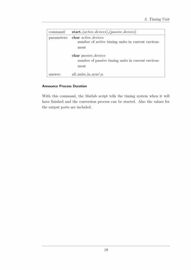
3.3.2 Send Packet

Transmits a UDP packet to a specified receive address and receive port. This

function requires a pointer to a bound transmit port. Commands, as specified

in Section 3.2.2, are sent to a timing unit via this function.

26

3. Timing Unit

function: Udp send(<pointer>,<remote IP>,<remote port>,

<data array>)

arguments: uint32 pointer

pointer that identifies the transmit port (in case of

a 64 bit operating system, this is of type uint64)

string remote IP

IP address of receiver

string remote port

port which receiver is listening to

string remote IP

IP address of receiver

uint8 data array

Matlab row vector that contains data to transmit

return value: none

3.3.3 Receive Packet

This function is used to receive return messages from a timing unit. It again

needs a pointer, like the send routine. The bound port is now the one the

function listens to.

function: Udp receive(<pointer>,<timeout>)

arguments: uint32 pointer

pointer that identifies the transmit port(in case of

a 64 bit operating system, this is of type uint64)

uint32 timeout

timeout value in ms

return value: [<error value>, <data>]

int8 error valuethis value reads one in case of error and zero oth-

erwise

27

3. Timing Unit

3.3.4 Close Port

When the bound UDP port is not required anymore, the port and allocated

memory from the bind process can be released with this function. This function

should be called at the end of the Matlab code.

function: Udp close(<pointer>)

arguments: uint32 pointer

pointer that identifies the bound port (in case of a

64 bit operating system, this is of type uint64)

return value: none

28

4. Performance Analysis

4 Performance Analysis

The first part of this chapter addresses the physical properties of the timing

unit. The parameters defined in the previous chapter are now compared to

the measured quantities of the implemented system. The second part discusses

the influence of the underlying network to the system characteristics.

4.1 Timing Unit Characteristics

4.1.1 Trigger Signal

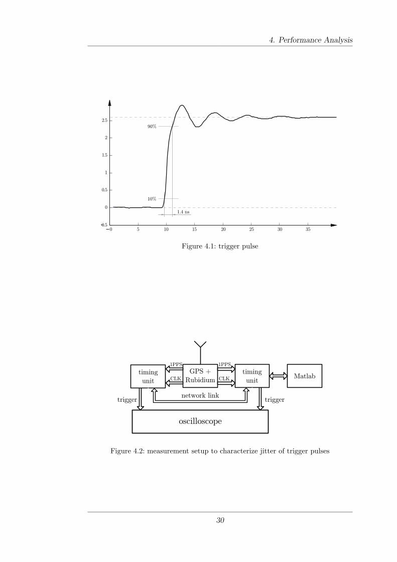
Relevant parameters of the trigger pulse are the rise time and voltage levels.

These two parameters can be seen in Figure 4.1, the pulse duration has to be

larger than one period of the clock signal. The trigger pulse is generated by the

CPLD and is therefore deterministic. The duration of the pulse corresponds

to the trigger granularity.

The pulse in Figure 4.1 has a rise time of approximately 1.4 ns and a level of

approximately 2.7 V for a logical one. These values were measured at a 50 Ω

load and fit well to the specification of the boards triggered by this pulses.

4.1.2 Jitter Analysis

The trigger pulses of two timing units should occur at the same time instant.

In a real system, it is not possible to generate pulses at exactly the same time.

29

4. Performance Analysis

−0 5 10 15 20 25 30 35−0.5

0

0.5

1

1.5

2

2.5

10%

90%

1.4 ns

Figure 4.1: trigger pulse

timingunit

GPS +Rubidium

1PPS

CLK

1PPS

CLKtimingunit

Matlab

network linktrigger trigger

oscilloscope

Figure 4.2: measurement setup to characterize jitter of trigger pulses

30

4. Performance Analysis

Nonetheless, if the jitter is small compared to the period of the reference clock,

the pulses can be considered synchronous. To verify this property, a setup as

shown in Figure 4.2 was used. The clock and the 1PPS signals for the two units

are derived from the same reference. Also the length of the signal cables is

equivalent for all units. In other words, the reference signals are synchronous

and the measured jitter is generated by the timing units only. The trigger

pulses of the units are captured by an oscilloscope and the time difference is

recorded. The result, after evaluating 108 pulses, is that the jitter is lower

than ±6 ps. Compared to the reference clock period of 5 ns (clock frequency

= 200 MHz), this value is small and therefore the pulses can be treated as

synchronous.

GPS +

Rubidium

1PPS

clktiming

unitMatlab

oscilloscope

clk triggertrigger

analog

signal

a/d

converter

Figure 4.3: measurement setup to verify if converter board is triggered correctly

The next test setup can be seen in Figure 4.3. The aim of this setup is to

measure the jitter between the trigger signal and the resulting analog signal

generated by the converter card. Only one timing unit and one converter

board is used. Both are clocked by the same reference. The signal output and

the trigger are connected to an oscilloscope. 105 trigger pulses are generated

(resulting in a measurement duration of approximately 28 hours). The result-

ing jitter between the analog signal and the trigger pulse is lower than ±0.5 ns

(reference clock period = 5 ns) and therefore the DAC always starts converting

at the same clock cycle relative to the trigger.

31

4. Performance Analysis

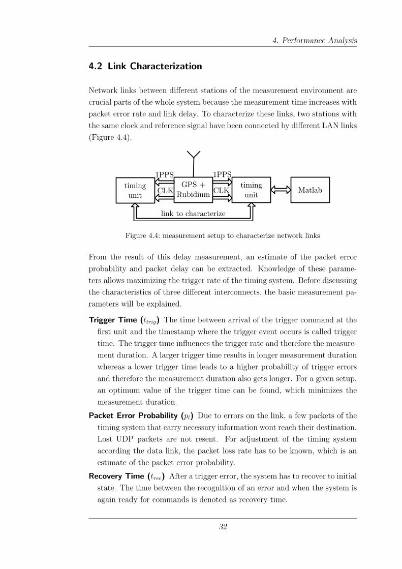
4.2 Link Characterization

Network links between different stations of the measurement environment are

crucial parts of the whole system because the measurement time increases with

packet error rate and link delay. To characterize these links, two stations with

the same clock and reference signal have been connected by different LAN links

(Figure 4.4).

timingunit

GPS +Rubidium

timingunit

Matlab

link to characterize

1PPS

CLK

1PPS

CLK

Figure 4.4: measurement setup to characterize network links

From the result of this delay measurement, an estimate of the packet error

probability and packet delay can be extracted. Knowledge of these parame-

ters allows maximizing the trigger rate of the timing system. Before discussing

the characteristics of three different interconnects, the basic measurement pa-

rameters will be explained.

Trigger Time (ttrig) The time between arrival of the trigger command at the

first unit and the timestamp where the trigger event occurs is called trigger

time. The trigger time influences the trigger rate and therefore the measure-

ment duration. A larger trigger time results in longer measurement duration

whereas a lower trigger time leads to a higher probability of trigger errors

and therefore the measurement duration also gets longer. For a given setup,

an optimum value of the trigger time can be found, which minimizes the

measurement duration.

Packet Error Probability (pl) Due to errors on the link, a few packets of the

timing system that carry necessary information wont reach their destination.

Lost UDP packets are not resent. For adjustment of the timing system

according the data link, the packet loss rate has to be known, which is an

estimate of the packet error probability.

Recovery Time (trec) After a trigger error, the system has to recover to initial

state. The time between the recognition of an error and when the system is

again ready for commands is denoted as recovery time.

32

4. Performance Analysis

Packet Delay In order to maximize the trigger rate and therefore minimize

the measurement time, the packet delay profile of the used link has to be

known. This profile has been measured with two timing units clocked by

the same reference and a special Matlab script. For analyzing the influence

to the measurement duration, the cumulative density function of the delay

profile has been evaluated. From this function the probability of error free

packet delivery, for a given trigger time, can be seen.

Timeout Duration (ttimeout) After a trigger process was initiated, the Matlab

script waits for a result message of the timing system. Due to lost packets,

this result might never arrive. The duration, after which the script aborts

the current trigger process, is called timeout duration.

Optimum Trigger Time To find the optimum trigger time for a given mea-

surement environment a cost function is used, which enables to understand

the influence of the parameters mentioned before to the total measurement

duration. Minimization of the cost function corresponds to maximization of

the trigger rate and therefore leads to a trigger time optimum in the sense

of minimum measurement duration.

4.2.1 Packet Loss Rate

All delay measurements were carried out by using two timing units (minimum

setup) and therefore parameters, like the packet loss rate of the link, could not

be measured directly.

pllllllll;1 pl;2

PC TU1 TU2

1 2

4 3

Figure 4.5: structure of the packet loss measurement

Figure 4.5 shows the structure of the packet loss measurement. The principle

idea is to send a ”trigger in zero” message, which can never result in a suc-

cessful trigger. This is because the trigger command needs some time to travel

from one timing unit via the network link to all others. As a result, the timing

33

4. Performance Analysis

system reports an error including the largest timing difference which corre-

sponds to the largest single trip time in the network. With this procedure, the

delay profile of the network link and the packet loss rate can be determined.

Several packets are sent in one measurement cycle (see Figure 4.5):

1: The PC tells its assigned timing unit (TU1) to immediately start a trigger.

PC and timing unit are directly connected via an Ethernet switch. Due

to this fact, the packet loss rate of this channel is lower than 10−6 and is

therefore set to zero.

pl,1 ≈ 0 (4.1)

2: The first timing unit forwards the trigger information to TU2. This is done

via a lossy channel (e.g. directive radio link) and therefore the packet loss

rate pl,2 is larger than zero.

3: Timing unit two reports an error including ∆t, the difference between the

announced trigger time instant and the time the trigger command was re-

ceived.

4: Timing unit one reports the timing difference to the PC.

Repeating this process and storing the results, allows to determine the packet

loss rate of the network link. It can be seen, that a measurement cycle is only

successful, if no packet in the chain (see Figure 4.5, lower part) is lost. A value

for pl,2 can be determined by

(1− Pmeas) = (1− pl,1)2(1− pl,2)2 (4.2)

where Pmeas is the measured error rate. Rearranging Equation (4.2) and in-

cluding Equation (4.1) results in

pl,2 = 1−√

(1− Pmeas) (4.3)

4.2.2 Packet Delay Profile

Not only the packet loss rate of a link is of interest because trigger packets

arriving too late are not useful any more and therefore produce an error. From

the delay measurement discussed in Section 4.2.1, the probability mass function

of the recorded delay values can be generated. In the next step a cumulative

mass function can be plotted which is more intuitive.

34

4. Performance Analysis

1 Pd

11

00

Pd

time time

Figure 4.6: packet delay profile

Figure 4.6 allows to determine the probability that a packet arrived within

a specific time value under the assumption that the packet is not lost. The

longer the available time, the higher the receive probability. The two graphs

in Figure 4.6 are equivalent, one shows the arrive probability and the other

depicts the error probability (packet delay is longer than desired duration).

For further calculations the packet delay error curve is used (right part of

Figure 4.6).

4.2.3 Trigger Process Duration

The result of a trigger process depends on the packets that are involved. For

example, packets can be lost or delayed. Only if all packets arrive within a

given time at their destination and none is lost, a trigger process can be suc-

cessful. As mentioned in the previous chapter, the link between the Matlab

script and its assigned timing unit is assumed to be ideal (both devices are

directly connected to the same network switch, therefore the loss rate will be

close to zero). It is assumed that every packet has the same error probability.

Indeed this is not true, because the error probability depends on the link. Sev-

eral different links can be used for interconnecting timing units. But assuming

the worst error rate to be present at all interconnects will deliver an upper

bound on the trigger process duration.

The number of packets involved in a trigger process can be calculated as follows

M active units send a trigger timestamp packet to all other (N − 1) units:

M(N− 1)

M active units have to receive a success message from all other units:

M(N− 1).

This leads to the equation

Np = 2M(N − 1) (4.4)

35

4. Performance Analysis

where M is the number of active timing units, N is the total number of units

and Np denotes the number of packets involved in one trigger process.

Successful Trigger Process A trigger process is only successful if:

No packet is lost ( p = (1− pl,2)Np),

all timestamp packets arrive within the trigger time

(p = (1− Pd(ttrig))Np2 ) and

all success messages arrive before the timeout occurs

(p = (1− Pd(ttimeout − ttrig))Np2 ).

The probability for a successful trigger event is therefore given by

psuccess = (1− pl,2)Np · (1− Pd(ttrig))Np2 · (1− Pd(ttimeout − ttrig))

Np2 . (4.5)

From Figure 4.7 it can be seen, that the average duration of a successful

trigger process is the combination of the execution time of the Matlab script

tM , the trigger time ttrig and the average conversion time ta/d.

tsuccess = tM + ttrig + ta/d (4.6)

signal generation signal transmission

time

triggertrigger ok

signal generation

tM ttrig ta/d

trigger

Figure 4.7: successful trigger process

Trigger Error If no packet is lost, but at least one did not arrive within the

trigger time, than at least one of the involved timing units could not trigger

at the right time instant and reports an error. The controlling Matlab script

receives the error message after a duration that equals approximately the

largest round trip time of the network (2ts). For this case the probability is

ptrigerror = (1− pl,2)Np · (1− (1− Pd(ttrig))Np2 ). (4.7)

The first term in this equation is the probability that no packet of the

trigger process is lost and the second term models the probability that at

36

4. Performance Analysis

least one trigger timestamp packet arrives too late (Np

2packets carry trigger

information, all others are used for status messages). The average duration

(see Figure 4.8) until a new trigger process can be started can be calculated

as

ttrigerror = tM + 2ts + trec. (4.8)

time

signal generation

trigger

signal generation recover

triggertrigger error

tM 2ts ta/d

Figure 4.8: trigger error due to delayed timestamp packet

Errors Caught by Timeout This part covers all the other errors that can oc-

cur. The probability can be calculated by

perror = 1− (psuccess + ptrigerror). (4.9)

The average duration (see Figure 4.9) is

terror = tM + ttimeout + trec. (4.10)

time

signal generationsignal generation recover

trigger

tM ttimeout trec

trigger

Figure 4.9: trigger error due to lost packet

Average Measurement Duration The average measurement duration tmeas

for I trigger processes can be calculated by

Ipsuccesstsuccess + Iptrigerrorttrigerror + Iperrorterror = tmeas. (4.11)

37

4. Performance Analysis

The number of successful trigger processes I is included in this equation by

the term

Ipsuccess = I. (4.12)

By combining the previous two equations, the measurement duration with

respect to the number of successful trigger processes (successful transmitted

data blocks) is calculated:

I

(tsuccess +

ptrigerrorttrigerror + perrorterror

psuccess

)= tmeas. (4.13)

If the duration of the Matlab script and the conversion process is fixed,

then the overall measurement duration is only influenced by the trigger

time ttrig, the timeout duration ttimeout and the characteristic of the link.

For determining the optimum trigger time, the number of parameters is

furthermore reduced by setting the timeout duration such that 99.999 % of

all packets arrive within this time.

Equation (4.13) can be rearranged to describe the number of trigger pro-

cesses per second (trigger rate)

1(tsuccess +

ptrigerrorttrigerror+perrorterror

psuccess

) =I

tmeas

(4.14)

Maximization of Equation (4.14) leads to an optimum value of ttrig (the same

result is achieved by minimizing Equation (4.13), but for the maximization

the cost function is bounded).

4.2.4 Optimum Trigger Time

For the calculation of the optimum trigger time, two Matlab scripts are nec-

essary. Both can be found on the attached CD1. The first program generates,

by the help of two timing units, a characteristic delay profile of a given net-

work link. Also the packet loss rate is recorded. The resulting workspace, that

contains all results, is stored to a hard disk. The next step is to specify all

necessary parameters in the second program and supply the path to the result

file. This program then calculates the optimum trigger time for the given link

1 Disk:\02 Data\05 Matlab\02 Optimum Trigger Time\

38

4. Performance Analysis

timing units involved 3active units 2

tM 45 msta/d 1 mstrec 10 ms

Table 4.1: example timing system parameters

and furthermore proposes a timeout duration. Also, the minimum achievable

trigger rate is calculated.

Example

Three timing units have to synchronize a system of converter boards using the

parameters listed in Table 4.1. The network link is done by two Linksys routers

in bridge mode. This is a low quality link, but the results of optimization can be

seen more clearly than with high end links. The link characteristic, including

delay profile and packet loss rate, has already been recorded as described above

and is loaded from the evaluation script. The script outputs an optimum

trigger delay value of 4.31 ms, which corresponds to 106 timer ticks. This is

the optimum value to be inserted into the ”trigger in x” function. Furthermore

a timeout duration of 10.73 ms is proposed.

Detailed information is shown in two graphs. Figure 4.10 shows the character-

istic delay profile of this setup and the vertical line marks the optimum value

of the trigger time. Figure 4.11 shows the achievable frame rate, corresponding

to three timing units and the parameters defined in Table 4.1. The highest

point in this curve is the optimum one, generating the minimum measurement

duration.

4.3 Link Timing Comparison

The Matlab program from the previous chapter can be used to determine the

optimum trigger duration for a given measurement setup. Three interconnects

have therefore been analyzed:

an optical fiber link

a directive radio link

and a WLAN link.

39

4. Performance Analysis

0 1 2 3 4 510

10

10

10

10

10

10

-6

-5

-4

-3

-2

-1

0

time/ms

del

ay p

robab

ility

Figure 4.10: delay profile: 802.11g WLAN link

0 20 40 60 80 100 120 140 1600

2

4

6

8

10

12

14

16

18

20

trigger time/ticks

fram

e ra

te /

fra

mes

per

sec

ond

Figure 4.11: achievable frame rate per trigger time

40

4. Performance Analysis

type ttrigger ttimeout packet error rate frame rateoptical fiber link 8 ticks 0.7 ms ≈ 0 21.6 fps

directive radio link 84 ticks 7.9 ms 6.2 10−6 19.7 fpsWLAN: 802.11g 106 ticks 10.7 ms 2.4 10−3 18.7 fpsWLAN: 802.11b 116 ticks 12.4 ms 2.2 10−2 15.2 fps

Table 4.2: results from the link timing analysis for tM = 45 ms

Results for the different links can be seen in Table 4.2. The parameters were

again chosen as in Table 4.1;

Detailed information on the links can be found in the chapters below.

4.3.1 Optical Fiber Connection

0 1 2 3 4 510

10

10

10

10

10

10

-6

-5

-4

-3

-2

-1

0

time/ms

del

ay p

robab

ility

Figure 4.12: delay profile: optical fiber connection

This connection consists of two transceivers, connected by an optical fiber

cable and is best suited for fast measurements because of its low delay and

low packet error rate. Another advantage of this system is that long distances

between two sites are possible. Figure 4.12 illustrates the trigger error profile.

4.3.2 Directive Radio Link

This system is a wireless bridge, that transparently interconnects two LAN

segments. Figure 4.12 shows the delay profile of this link.

41

4. Performance Analysis

0 1 2 3 4 510

10

10

10

10

10

10

-6

-5

-4

-3

-2

-1

0

time/ms

del

ay p

robab

ility

Figure 4.13: delay profile: directive radio link

4.3.3 Low-Cost WLAN Connection

0 1 2 3 4 510

10

10

10

10

10

10

-6

-5

-4

-3

-2

-1

0

time/ms

del

ay p

robab

ility

802.11b

802.11g

Figure 4.14: delay profile: WLAN connection

In comparison to the links discussed before, a low cost connection established

by standard home or office use WLAN routers was characterized. The results

can be seen in Figure 4.14. For measurement setups, which require only low

trigger rates, this is a cheap alternative.

42

4. Performance Analysis

type ttrigger ttimeout packet error rate frame rateoptical fiber link 6 ticks 0.7 ms ≈ 0 233.1 fps

directive radio link 84 ticks 7.9 ms 6.2 10−6 112.9 fpsWLAN: 802.11g 97 ticks 10.4 ms 2.4 10−3 98.5 fpsWLAN: 802.11b 115 ticks 12.4 ms 2.2 10−2 64.8 fps

Table 4.3: results from the link timing analysis for tM = 3 ms

4.4 Discussion of the Results

Table 4.2 shows the results from the link timing analysis for an average Matlab

duration tM of 45 ms. This value is realistic, if data processing is necessary

between two consequent transmissions (trigger processes). In this case the

Matlab duration is much larger than the trigger time ttrigger and therefore the

frame rate is mainly determined by 1/tM = 22.2 fps.

If the data to transmit is precalculated and only has to be loaded to the

transmit buffer of the D/A converter board, then the Matlab duration tM

decreases to roughly 3 ms (for ta/d = 1 ms, 4 channels with 200 Msamples/s,

2 bytes per sample) which is in the range of the trigger time ttrigger. In this case

the performance spread between the different network links is huge (compare

Table 4.2 Table 4.3).

43

5. Conclusion

5 Conclusion

In this thesis, a system was developed that allows synchronization of several

sites of a telecommunication rapid prototyping system. A 50 Ω output available

at the so called ”timing unit” was used to trigger the A/D and D/A converter

boards. The synchronous trigger pulses were generated by a distributed system

consisting of several timing units. Each unit is mainly a CPLD in combination

with a 32-bit ARM microcontroller. All time critical parts of the system were

implemented in the CPLD whereas the microcontroller was responsible for

communication issues. A flexible interface for controlling the timing system,

via UDP messages, was introduced as well as a set of MEX functions for easy

integration of the system into existing Matlab codes. Finally, the performance

of the designed system was analyzed by testing it under real world conditions.

The measurement results perfectly match the predicted behavior of the system

and it is therefore well suited for high precision synchronization problems.

44

Bibliography

Bibliography

[1] V. Jungnickel, T. Wirth, M. Schellmann, T. Haustein, and W. Zirwas, “Synchronization

of cooperative base stations,” in Wireless Communication Systems. 2008.ISWCS ’08. IEEE International Symposium on, pp. 329 –334, oct. 2008, doi:10.1109/ISWCS.2008.4726071.

[2] Keil, “Mcb2300 evaluation board,” 2008.http://www.keil.com/mcb2300/

[3] NXP, “An10799 - uip webserver source code,” 2008.http://www.nxp.com/documents/other/uip webserver src.zip

[4] NXP, “Porting uip1.0 to lpc23xx/24xx,” 2009.http://www.nxp.com/documents/application note/AN10799.pdf

[5] S. Donnelly, “Endance dag time-stamping whitepaper,” White paper, EndanceTechnology Ltd., 2006, available online (8 pages).http://www.endace.com

[6] S. Caban, “Development and setting up of a 4x4 real-time mimo testbed,” Institutfur Nachrichtentechnik und Hochfrequenztechnik, 2005.http://publik.tuwien.ac.at/files/pub-et 9754.pdf

45