Embed Size (px)
Citation preview
User Guide
GDDGraphic Data Display
2 GDD User Guide
Copyright
© European Union, 1995‐2014
Reproduction is authorised, provided the source is acknowledged, save where otherwise stated.
Where prior permission must be obtained for the reproduction or use of textual and multimedia information (sound, images, software, etc.), such permission shall cancel the above‐mentioned general permission and shall clearly indicate any restrictions on use.
Disclaimer
On any of the MARS pages you may find reference to a certain software package, a particular contractor, or group of contractors, the use of one or another sensor product, etc. In all cases, unless specifically stated, this does not indicate any preference of the Commission for that particular product, party or parties. When relevant, we include links to pages that give you more information about the references.
Feel free to contact us, in case you need additional explanations or information.
Release Issue Date
1 3 June 2014
1
Contents
1 Help contents 3Credits . . . . . . . . . . . . . . . . . . . . . . . . . . . . . . . . . . . . . . . . . . . . . . . . . . . . . . . . . . . . . . . . . . . . . . . . . . 4
2 Using GDD 5About GDD . . . . . . . . . . . . . . . . . . . . . . . . . . . . . . . . . . . . . . . . . . . . . . . . . . . . . . . . . . . . . . . . . . . . . . 6
Installing and launching GDD . . . . . . . . . . . . . . . . . . . . . . . . . . . . . . . . . . . . . . . . . . . . . . . . . . . . . . . 8Installation prerequisites . . . . . . . . . . . . . . . . . . . . . . . . . . . . . . . . . . . . . . . . . . . . . . . . . 8Launching the application. . . . . . . . . . . . . . . . . . . . . . . . . . . . . . . . . . . . . . . . . . . . . . . . . 8
Workspace overview . . . . . . . . . . . . . . . . . . . . . . . . . . . . . . . . . . . . . . . . . . . . . . . . . . . . . . . . . . . . . . 9
Available data views. . . . . . . . . . . . . . . . . . . . . . . . . . . . . . . . . . . . . . . . . . . . . . . . . . . . . . . . . . . . . . 12Tabular view vs. Graph views . . . . . . . . . . . . . . . . . . . . . . . . . . . . . . . . . . . . . . . . . . . . . . . . 12Tabular view . . . . . . . . . . . . . . . . . . . . . . . . . . . . . . . . . . . . . . . . . . . . . . . . . . . . . . . . . . . . . . 13Graph Var vs Time view . . . . . . . . . . . . . . . . . . . . . . . . . . . . . . . . . . . . . . . . . . . . . . . . . . . . . 15Graph Var vs Var view . . . . . . . . . . . . . . . . . . . . . . . . . . . . . . . . . . . . . . . . . . . . . . . . . . . . . . 16Histograms view. . . . . . . . . . . . . . . . . . . . . . . . . . . . . . . . . . . . . . . . . . . . . . . . . . . . . . . . . . . 17Graph Soil Profile view . . . . . . . . . . . . . . . . . . . . . . . . . . . . . . . . . . . . . . . . . . . . . . . . . . . . . 18Graph Micale . . . . . . . . . . . . . . . . . . . . . . . . . . . . . . . . . . . . . . . . . . . . . . . . . . . . . . . . . . . . . 20Frequency view . . . . . . . . . . . . . . . . . . . . . . . . . . . . . . . . . . . . . . . . . . . . . . . . . . . . . . . . . . . 22
Using the GDD auto‐draw capabilities . . . . . . . . . . . . . . . . . . . . . . . . . . . . . . . . . . . . . . . . . . . . . . . 23Creating a new configuration . . . . . . . . . . . . . . . . . . . . . . . . . . . . . . . . . . . . . . . . . . . . . . . . 23Loading a saved configuration . . . . . . . . . . . . . . . . . . . . . . . . . . . . . . . . . . . . . . . . . . . . . . . 25Editing and saving a configuration . . . . . . . . . . . . . . . . . . . . . . . . . . . . . . . . . . . . . . . . . . . . 27Comparing the results with existing reference data . . . . . . . . . . . . . . . . . . . . . . . . . . . . . . 28Exporting the graph. . . . . . . . . . . . . . . . . . . . . . . . . . . . . . . . . . . . . . . . . . . . . . . . . . . . . . . . 31

CONTENTS
2 GDD User Guide
GDD User Guide 3
1Help contents
This Guide is targeted to advanced users of the BioMA Software Framework.
In particular, this Help describes how to use GDD (Graphic Data Display), a Microsoft .NET component, which allows displaying the simulation results either as textual tables or as graphs.
The topics are organized as follows:
See also:
• BioMA Framework User Guide (http://bioma.jrc.ec.europa.eu/bioma/help/)
• “Credits” on page 4
Topic Contents
“About GDD” on page 6 A general introduction to the application’s features
“Installing and launching GDD” on page 8
How to install and launch Graphic Data Display
“Workspace overview” on page 9
An overview of the application’s user interface and main functions
“Available data views” on page 12
Examples of the tabular and graphic data views
“Using the GDD auto‐draw capabilities” on page 23
How to use the application to create and manage the graph data views
Tip:
To access the Web portal of BioMA go to http://bioma.jrc.ec.europa.eu/
1 – HELP CONTENTS
4 GDD User Guide
Credits
The current version of CRA.Core.GDD was developed by CRA‐ISCI (Agriculture Research Center) within the project SEAMLESS (EU ‐ DG Research, contract no. 010036‐2)
See http://www.seamless‐ip.org
Development
• Marcello Donatelli
• Andrea Di Guardo
Programming
• Andrea Di Guardo
• Marcello Donatelli
Download
This component is made available free of charge to non profit users. You will need to contact CRA‐CIN at [email protected]‐cin.it if you intend to use CRA.Core.GDD in profit‐related applications.
The current version of the software can be downloaded here
References
Di Guardo A., M. Donatelli M., M. Botta, 2007. Two framework components to simulate biophysical systems. Proc. of Farming Systems Design 2007, Catania, Italy, 10‐12 September, 2007.
GDD User Guide 5
2Using GDD
This topic is organized into the following sections:
• “About GDD” on page 6
• “Installing and launching GDD” on page 8
• “Workspace overview” on page 9
• “Available data views” on page 12
• “Using the GDD auto‐draw capabilities” on page 23
2 – USING GDD
6 GDD User Guide
About GDD
Scope
Providing data views via graphical user interfaces is a common need for every application built to make use of models.
If model output is generated by a modular system in which model components are interchangeable, output variables may change; thus, maintaining such graphical user interfaces, can be challenging and resource demanding.
A tool which can load datasets with various schema and which helps the user to visualize data in various ways, it would speed up application development, allowing focusing on models, rather than on user interfaces. In such a tool, whether flexibility of use is a need, providing domain specific views of data would add value both in operational use and in model development.
What GDD can be used for
GDD (Graphic Data Display) is a Microsoft .NET component, which has the specific purpose to retrieve a set of output variables and to allow displaying values either by textual tables or by several kinds of graphs.
Also, reference data (e.g., data from experiments, or surveys) can be superimposed to simulation results. Graphs can be saved as image files. GDD can be used as a stand‐alone tool or as a component inside an application (see “GDD as a BioMA plugin” on page 7).
In the former case it provides access to a file dialog to allow the user selecting a file, whereas in the latter case it can be opened inside a modeling framework directly loading the current dataset.
Data formats
At this development stage, GDD accepts inputs via three different formats: XML, Microsoft Excel, and a more compact/faster binary (another component, also available, allows I/O operations with the binary format). Readers can however be extended by third parties implementing the proper interface.
Each variable can be either a table column, or an entire table of the dataset, depending on the fact that it is either only time‐variant or time and 1 dimension space‐variant (the latter are variables that vary across soil profiles, such as soil temperature).
7
ABOUT GDD
GDD User Guide
GDD as a BioMA plugin
Besides of being a stand‐alone application, GDD can be used as a BioMA plug‐in.
Users can access it from within the BioMA Graphical User Interfaces (Spatial and Point) so as to load the current dataset and visualize data both in tabular and graphical form.
Related topics:
• “Installing and launching GDD” on page 8
• “Workspace overview” on page 9
• “Available data views” on page 12
• “Using the GDD auto‐draw capabilities” on page 23
Tip:
For further information on how to use GDD as a BioMA plugin, see the BioMA Spatial User Guide (http://bioma.jrc.ec.europa.eu/spatial/help/) .
2 – USING GDD
8 GDD User Guide
Installing and launching GDD
Installation prerequisites
In order to install and run Graphic Data Display, the following prerequisites must be fulfilled:
Hardware prerequisites
• Operative system: Windows XP/Vista/7 (32 or 64 bit)
Software prerequisites
The following software must be installed on your computer:
• NET 3.5 Framework ‐ To install it, click here. Follow the product’s documentation, if needed.
Regional Settings of your PC
Ensure that the Regional Settings of your PC are set as follows:
1 Access the Windows Control Panel (Start > Control Panel > Clock, Language, and Region > Region and Language).
2 In the Region and Language window, click Additional settings.
3 Be sure that the Decimal symbol is set to “point” (.).
Launching the application
As a stand-alone tool:
Download it from the BioMA Components Web portal:
1 In your browser, go to http://bioma.jrc.ec.europa.eu/components/default.aspx?productname=gdd.
2 Select GDD, click Install from URL and then follow the instructions.
As a BioMA plugin:
• After running a model simulation and launching the Simulation Result Visualizer, open it by clicking the Open tables with GDD button.
• Load the current dataset to visualize data.
Related topics:
• “Workspace overview” on page 9
9
WORKSPACE OVERVIEW
GDD User Guide
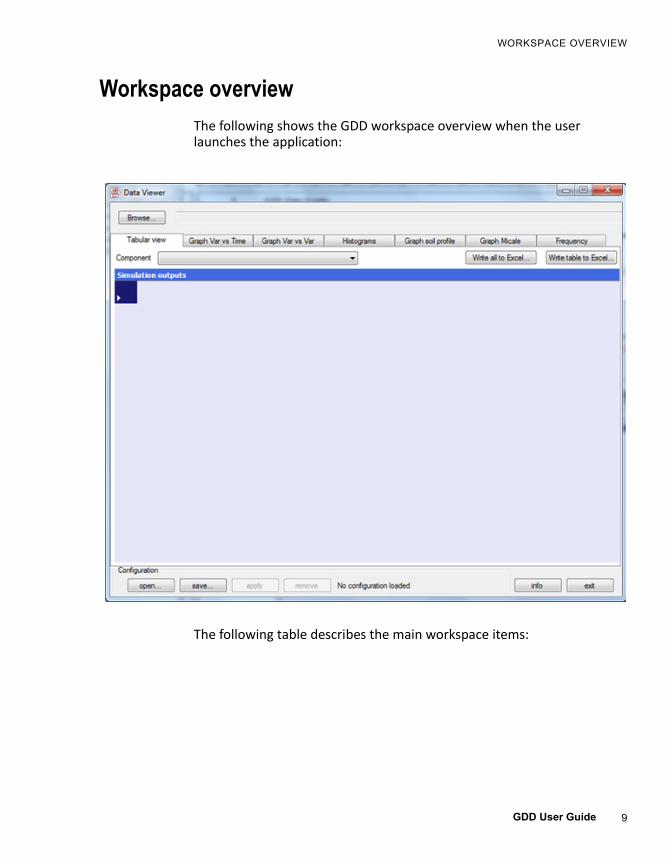
Workspace overviewThe following shows the GDD workspace overview when the user launches the application:
The following table describes the main workspace items:
2 – USING GDD
10 GDD User Guide
Workspace item Description
TABS
Tabular view
It allows selecting a single table from the dataset and visualizing its content on screen.
From this data view, single tables (or all tables at once) can be saved in a Microsoft Excel format, using the ad‐hoc buttons. See “Tabular view” on page 13.
Graph Var vs Time
It provides the opportunity to plot up to seven variables vs. time allowing the user to set the time period and providing some graph options. See “Graph Var vs Time view” on page 15.
Graph Var vs VarIt allows plotting a variables of choice vs. another variable. “Graph Var vs Var view” on page 16.
HistogramsIt allows plotting histograms on graphs which do not have time explicit. See “Histograms view” on page 17.
Graph soil profile
This tab is only available if the model’s output includes the soil data and it allows plotting the variables that relate to soil.
This is a domain specific graphical representation of a selection of variables generally available in a biophysical system simulation. See “Graph Soil Profile view” on page 18.
Graph MicaleIt is a graphic metaphor which allows plotting daily values of an output variable using a scale of colours. See “Graph Micale” on page 20.
FrequencyIt shows the distribution of values in a number of classes chosen by the user. See “Frequency view” on page 22.
11
WORKSPACE OVERVIEW
GDD User Guide
Related topics:
• “Available data views” on page 12
• “Using the GDD auto‐draw capabilities” on page 23
BUTTONS
BrowseIt allows loading the XML(s) files that include the dataset(s).
Component It allows selecting the component to visualize.
Write all to Excel
Only relevant for the Tabular view tab.
It allows saving all tables in a Microsoft Excel format, in one single operation.
Write table to Excel
Only relevant for the Tabular view tab.
It allows saving a single table in a Microsoft Excel format.
Configuration
• Open ‐ It allows loading an existing configuration, that is, a graph that you have already created and saved.
• Save ‐ It allows saving a configuration, that is, variables and settings of a graph. Using this function you can reuse a graph configuration.
• Apply ‐ It allows viewing a saved graph.
• Remove ‐ It removes the loaded configuration.
For further information on using these buttons, refer to “Using the GDD auto‐draw capabilities” on page 23.
InfoIt shows information on the software release and allows accessing this Help.
Exit It closes the application.
Workspace item Description
2 – USING GDD
12 GDD User Guide
Available data viewsEach tab of the GDD Graphical User Interface, provides a different type of data view.
This topic provides a general overview of each data view, as well as some examples of graphs.
Tabular view vs. Graph views
GDD allows displaying values either by textual tables or by several kinds of graphs.
On each of the graph types available, variables can be selected and plotted.
However, automatic plotting can be activated loading GDD files with the information needed to use the auto‐draw feature. Such files can be built via GDD.
The use cases related to this feature of GDD are described in “Using the GDD auto‐draw capabilities” on page 23.
See also:
• “Tabular view” on page 13
• “Graph Var vs Time view” on page 15
• “Graph Var vs Var view” on page 16
• “Histograms view” on page 17
• “Graph Soil Profile view” on page 18
• “Graph Micale” on page 20
• “Frequency view” on page 22
• “Using the GDD auto‐draw capabilities” on page 23
Note:
The auto-draw configurations are specific to the input file content.
13
AVAILABLE DATA VIEWS
GDD User Guide
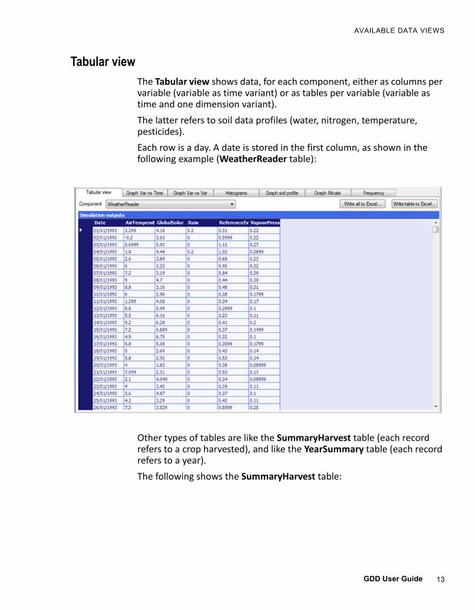
Tabular viewThe Tabular view shows data, for each component, either as columns per variable (variable as time variant) or as tables per variable (variable as time and one dimension variant).
The latter refers to soil data profiles (water, nitrogen, temperature, pesticides).
Each row is a day. A date is stored in the first column, as shown in the following example (WeatherReader table):
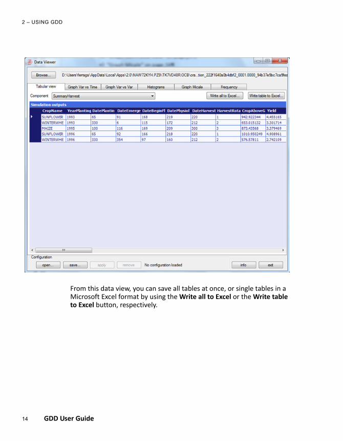
Other types of tables are like the SummaryHarvest table (each record refers to a crop harvested), and like the YearSummary table (each record refers to a year).
The following shows the SummaryHarvest table:
2 – USING GDD
14 GDD User Guide
From this data view, you can save all tables at once, or single tables in a Microsoft Excel format by using the Write all to Excel or the Write table to Excel button, respectively.
15
AVAILABLE DATA VIEWS
GDD User Guide
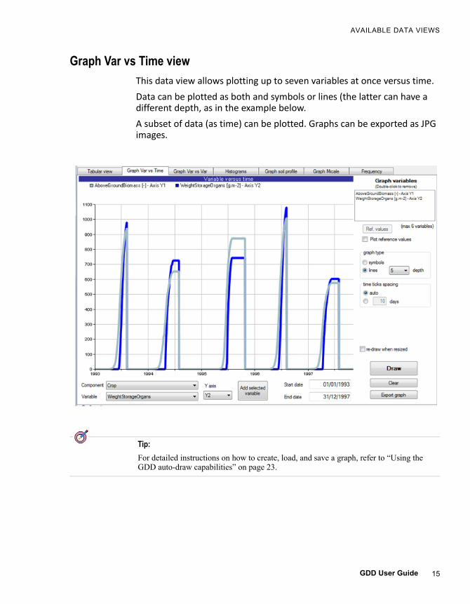
Graph Var vs Time viewThis data view allows plotting up to seven variables at once versus time.
Data can be plotted as both and symbols or lines (the latter can have a different depth, as in the example below.
A subset of data (as time) can be plotted. Graphs can be exported as JPG images.
Tip:
For detailed instructions on how to create, load, and save a graph, refer to “Using the GDD auto-draw capabilities” on page 23.
2 – USING GDD
16 GDD User Guide
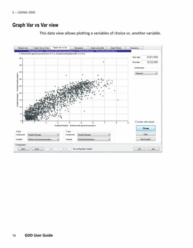
Graph Var vs Var viewThis data view allows plotting a variables of choice vs. another variable.
17
AVAILABLE DATA VIEWS
GDD User Guide
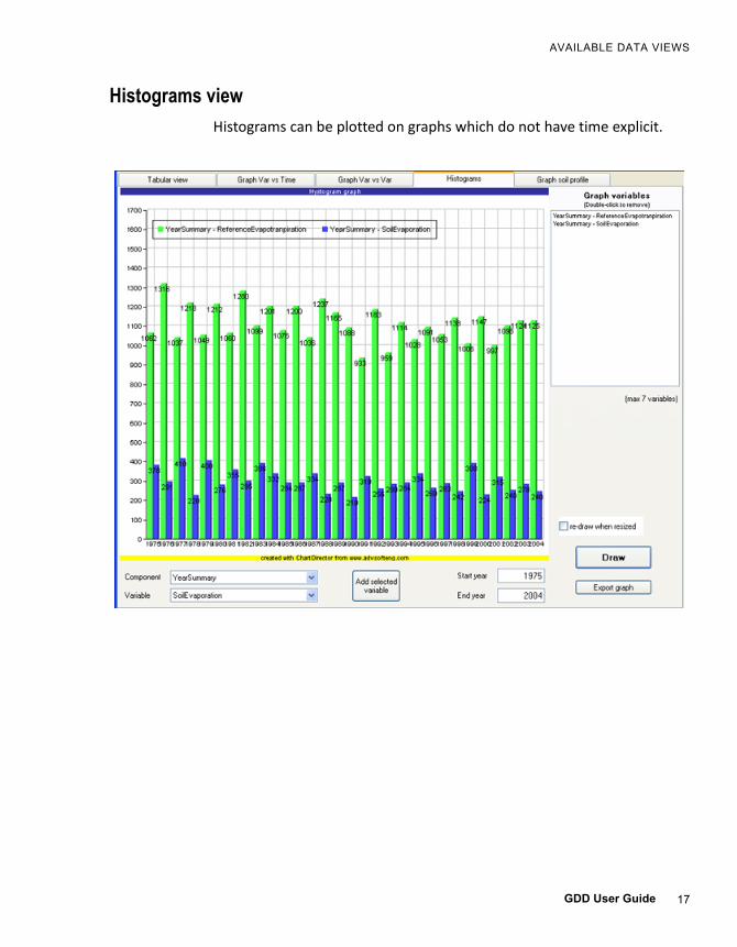
Histograms viewHistograms can be plotted on graphs which do not have time explicit.
2 – USING GDD
18 GDD User Guide
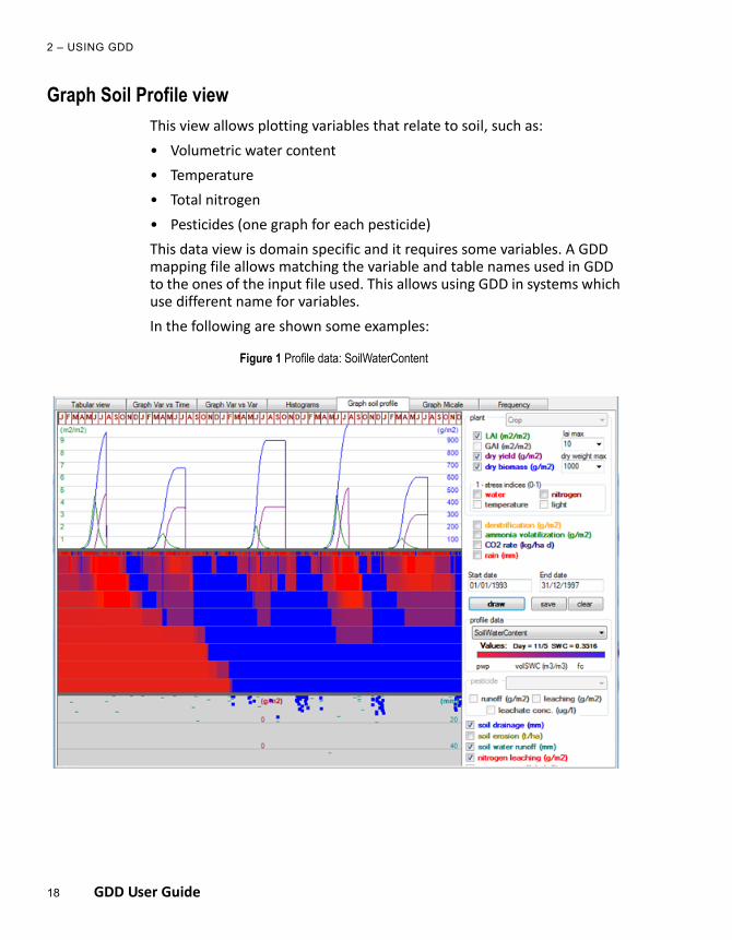
Graph Soil Profile viewThis view allows plotting variables that relate to soil, such as:
• Volumetric water content
• Temperature
• Total nitrogen
• Pesticides (one graph for each pesticide)
This data view is domain specific and it requires some variables. A GDD mapping file allows matching the variable and table names used in GDD to the ones of the input file used. This allows using GDD in systems which use different name for variables.
In the following are shown some examples:
Figure 1 Profile data: SoilWaterContent
19
AVAILABLE DATA VIEWS
GDD User Guide
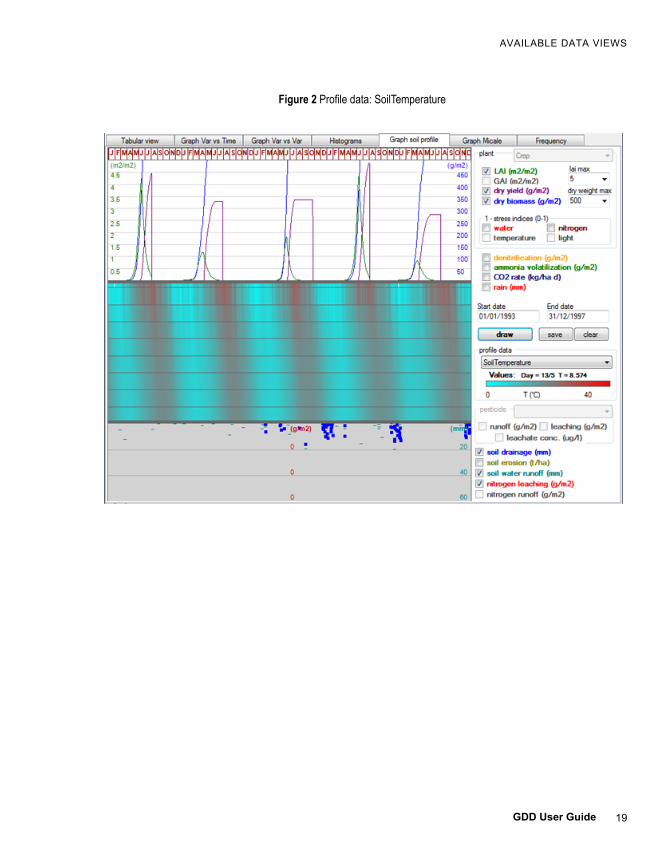
Figure 2 Profile data: SoilTemperature
2 – USING GDD
20 GDD User Guide
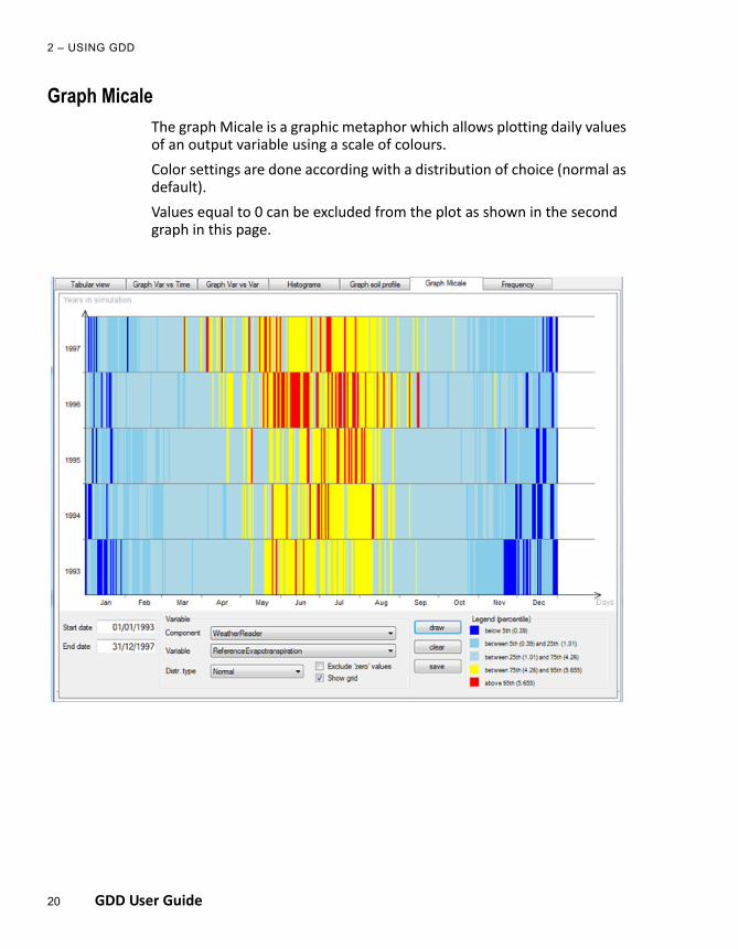
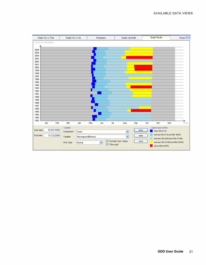
Graph MicaleThe graph Micale is a graphic metaphor which allows plotting daily values of an output variable using a scale of colours.
Color settings are done according with a distribution of choice (normal as default).
Values equal to 0 can be excluded from the plot as shown in the second graph in this page.
21
AVAILABLE DATA VIEWS
GDD User Guide
2 – USING GDD
22 GDD User Guide
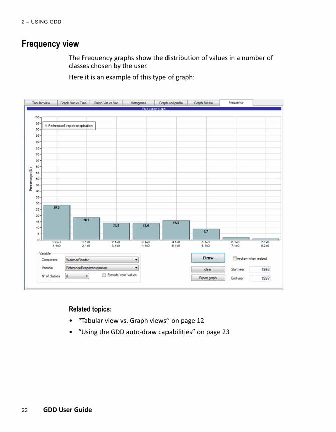
Frequency viewThe Frequency graphs show the distribution of values in a number of classes chosen by the user.
Here it is an example of this type of graph:
Related topics:
• “Tabular view vs. Graph views” on page 12
• “Using the GDD auto‐draw capabilities” on page 23
23
USING THE GDD AUTO-DRAW CAPABILITIES
GDD User Guide
Using the GDD auto-draw capabilitiesThis section describes how to use GDD to visualize, create, and edit variable configurations that are used to view data as graphs.
You can load a configuration from any of the available tabs.
To run operations related to auto‐draw, specific buttons are provided at the bottom of the form.
In particular:
• “Creating a new configuration” on page 23
• “Loading a saved configuration” on page 25
• “Editing and saving a configuration” on page 27
• “Comparing the results with existing reference data” on page 28
• “Exporting the graph” on page 31
Creating a new configuration
To create a new configuation:
1 Click Browse at the top of the GDD window.
2 Select the XMLs that contains the dataset(s) and click Open.
3 Select the Graph view tab you want to configure and then select a Component from the dropdown list. In this example we select Graph Var vs Time.
4 Set the Variable you want to use from the dropdown list, and then set the graph’s Axis.
5 Click Add selected variable. The variable is added in the Graph variables pane at the top‐right.
You can add as many variables as it is indicated. To remove a variable, double‐click it.
6 Set the other parameters, as required:
‐ Start date and End date ‐
Note:
If you are using GDD as a BioMA plugin, the Browse button is not available as, in this case, GDD is opened inside a modeling framework directly loading the current dataset.
2 – USING GDD
24 GDD User Guide
‐ Ref. Values ‐ This button becomes available after selecting a variable in the Graph variables list. If you have reference values, you can use this function to compare the simulation results with existing reference data. For further information, see “Comparing the results with existing reference data” on page 28.
‐ Plot reference values ‐ Check to enable the capability.
‐ Graph type ‐ Select the graph type you want to generate. If you select Lines, you can also set the depth.
‐ Time ticks spaces ‐ Set the value (Auto or select a value from the dropdown list).
‐ Re‐draw when resized ‐ Select this checkbox to properly resize the graph when the graph area changes (e.g., the GDD window is resized).
7 Once finished, click Draw to display the graph. To clear the graph from the form click Clear.
8 Click the Save button.
9 In the text box that popups, specify the modelling solution/type of output file the configuration is made for. (Recommended).
10 Close the text box. The configuration has been saved and you can now reload for a future use/edit. (See “Loading a saved configuration” on page 25).
11 You can also save your graph as an image by clicking the Export graph button. Available formats are: JPG, PNG, GIF, and BMP.
Related topics:
• “Loading a saved configuration” on page 25
• “Editing and saving a configuration” on page 27
• “Comparing the results with existing reference data” on page 28
• “Exporting the graph” on page 31
Note:
The Save button allows saving the current choice of variables for each tab. All tabs are saved at once.
25
USING THE GDD AUTO-DRAW CAPABILITIES
GDD User Guide
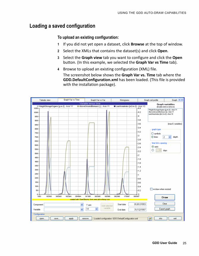
Loading a saved configuration
To upload an existing configuration:
1 If you did not yet open a dataset, click Browse at the top of window.
2 Select the XMLs that contains the dataset(s) and click Open.
3 Select the Graph view tab you want to configure and click the Open button. (In this example, we selected the Graph Var vs Time tab).
4 Browse to upload an existing configuration (XML) file.
The screenshot below shows the Graph Var vs. Time tab where the GDD.DefaultConfiguration.xml has been loaded. (This file is provided with the installation package).
2 – USING GDD
26 GDD User Guide
Related topics:
• “Creating a new configuration” on page 23
• “Editing and saving a configuration” on page 27
• “Comparing the results with existing reference data” on page 28
• “Exporting the graph” on page 31
27
USING THE GDD AUTO-DRAW CAPABILITIES
GDD User Guide
Editing and saving a configurationYou can load an existing configuration and use it as a basis to create a new one:
1 Click the Open button and then load an existing configuration (see “Loading a saved configuration” on page 25).
2 There are two possible scenarios:
a. If you already opened a dataset, the graph will be displayed after selecting the configuration.
b. If you did not opened a dataset, click Browse, select it (see “Loading a saved configuration” on page 25) and then click Apply to view the graph.
3 Edit your settings as needed (add/remove variables, change the graph type, and so forth).
4 Click the Save button.
5 In the text box that popups, enter a meaningful description for the configuration, and then close it.
6 In the Save as dialog that is displayed, enter a new name for your configuration and click Save.
Related topics:
• “Creating a new configuration” on page 23
• “Loading a saved configuration” on page 25
• “Comparing the results with existing reference data” on page 28
• “Exporting the graph” on page 31
2 – USING GDD
28 GDD User Guide
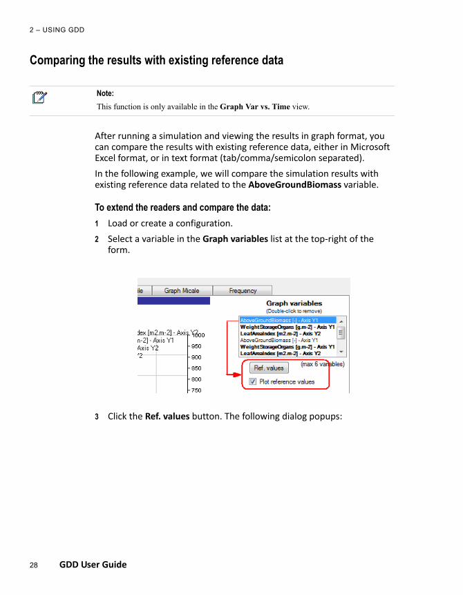
Comparing the results with existing reference data
After running a simulation and viewing the results in graph format, you can compare the results with existing reference data, either in Microsoft Excel format, or in text format (tab/comma/semicolon separated).
In the following example, we will compare the simulation results with existing reference data related to the AboveGroundBiomass variable.
To extend the readers and compare the data:
1 Load or create a configuration.
2 Select a variable in the Graph variables list at the top‐right of the form.
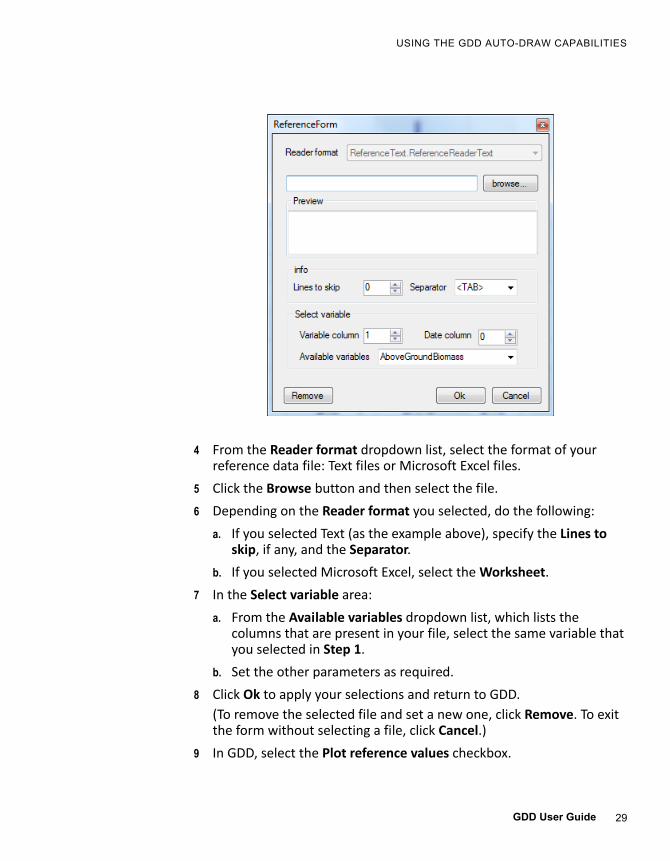
3 Click the Ref. values button. The following dialog popups:
Note:
This function is only available in the Graph Var vs. Time view.
29
USING THE GDD AUTO-DRAW CAPABILITIES
GDD User Guide
4 From the Reader format dropdown list, select the format of your reference data file: Text files or Microsoft Excel files.
5 Click the Browse button and then select the file.
6 Depending on the Reader format you selected, do the following:
a. If you selected Text (as the example above), specify the Lines to skip, if any, and the Separator.
b. If you selected Microsoft Excel, select the Worksheet.
7 In the Select variable area:
a. From the Available variables dropdown list, which lists the columns that are present in your file, select the same variable that you selected in Step 1.
b. Set the other parameters as required.
8 Click Ok to apply your selections and return to GDD.
(To remove the selected file and set a new one, click Remove. To exit the form without selecting a file, click Cancel.)
9 In GDD, select the Plot reference values checkbox.
2 – USING GDD
30 GDD User Guide
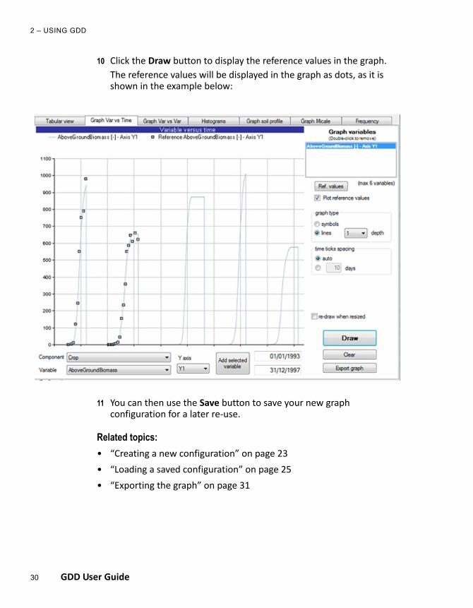
10 Click the Draw button to display the reference values in the graph.
The reference values will be displayed in the graph as dots, as it is shown in the example below:
11 You can then use the Save button to save your new graph configuration for a later re‐use.
Related topics:
• “Creating a new configuration” on page 23
• “Loading a saved configuration” on page 25
• “Exporting the graph” on page 31
31
USING THE GDD AUTO-DRAW CAPABILITIES
GDD User Guide
Exporting the graphAll graphs can be exported as an image by doing the following:
1 Once you are finished drawing your graph, click the Export graph button at the bottom of the window.
2 In the window that is displayed, select the image format (JPG, GIF, PNG, or BMP) from the Save as type dropdown list.
3 Specify a File name and then click Save.
Related topics:
• “Creating a new configuration” on page 23
• “Available data views” on page 12

2 – USING GDD
32 GDD User Guide