TRANSPORTATION RESEARCH RECORD 1172 23

Generalized Loglinear Models of Truck Accident Rates

F. F. 5ACCOMANNO AND C. BUYCO

Several methods for calibrating statistical models of truck accident rates are considered. A loglfnear approach Is sug­gested for assessing the effect of traffic environment on truck accident rates. A number of concerns assoclated with using a weighted least squares algorithm for estimating ~ parameters in the logllnear expression are noted, l.ncludlng the presence of reduced cell membership in the contingency tables of accidents and input variable lncompatlbllJtles between continuous ex­posure and categorical accident measures. An alternative form of generalized linear Interactive model (GLIM) Is proposed for calibrating logUnear expressions of truck accident rates. GLIM uses maximum Ukellhood techniques for estlmatlng ~ parameters In logllnear expressions. As In the classical weighted least squares algorithm, this approach permits a stepwise statistical analysis of higher-order lnteractlons In the traffic envJronment as related to accident frequencies, while adjusting directly for continuous measures of exposure. The resuJts of a calibration of GLIM logllnear expressions are presented using 1983 truck accident and exposure data for Ontario as a basis.

Truck accidents are caused by complex interactions of environ­mental and operational factors that are present at a specific time and location on the road network. Higher-order interactions between mitigating factors in an accident situation can be identified through a calibration of statistical models of truck accident rates. These rates are usually expressed as the ratio of the number of accidents divided by the amount of travel for a comparable mix of mitigating factors. The amount of travel or exposure measure reflects the number of opportunities avail­able for each accident to take place (I).

Recent attempts to calibrate reliable statistical models of truck accident rates have been hampered by two basic con­cerns: (a) incompatibility between continuous exposure infor­mation and categorical accident data and (b) the absence, in most jurisdictions, of comprehensive information on truck ex­posure. fucompatibilities in variable inputs restrict the meth­odology for analyzing truck accident rates to procedures that can incorporate both categorical and continuous information directly into the analysis. The absence of suitable exposure information has restricted the classification of accident en­virorunent to basic conditions for which travel information is available. Frequently, this has resulted in an analysis of factors that ignores second- and third-order interactions that affect truck accident rates. A number of recent studies on truck accidents illustrate the problems associated with lack of ex­posure data and incompatibilities in factor inputs for truck accident rate models (2-4).

Department of Civil Engineering, University of Waterloo, Waterloo, Ontario N2L 3Gl, Canada.

In this paper, some previous methods of analysis for truck accident rates are explored. The discussion is methodological in nature, with emphasis on the major limitations associated with each approach. Some important statistical concerns for the use of classical loglinear models in truck accident rate analysis are addressed. Alternatively, a generalized linear interactive model (GLIM) form of loglinear expression that incorporates both categorical accident involvement data and continuous exposure measures is suggested As does the classical loglinear model, this approach allows for a stepwise statistical analysis of higher-order interaction effects for truck accidents, while adjusting directly for the continuous exposure factor.

ALTERNATIVE METHODS OF ANALYSIS

In recent years, the issue of truck safety has been receiving considerable attention. However, both the methods of analysis and many of the conclusions from these studies have lacked consistency. A special report on twin trailer trucks (doubles) by TRB (5) reviewed the available literature on truck safety in the United States and reported that " ... several studies are ex­tremely variable and conflicting." A recent presentation of results to an Organization for Economic Cooperation and De­velopment meeting of member countries (6) and an earlier review by Freitas (7) arrived at similar conclusions. Much of the blame for a lack of consistency in studies of truck accidents has been attributed to limitations in the available data in various jurisdictions.

The focus of the discussion in this section of the paper is on methodology rather than results in recognition that the results may not be transferable to all jurisdictions. A lack of consis­tency in the choice of analysis procedure may have contributed as much to conflicting evidence on truck accident causation as problems with the data bases did.

In this section, three different procedures for calibrating truck accident rate expressions are discussed. The purpose of these expressions is to give a mathematical representation of the relationship between factors that influence accidents and the resultant truck accident rates. Mitigating factor inputs for these expressions are obtained from a statistical screening of candidate variables by multivariate techniques, such as analysis of variance and factor analysis.

Multiple Linear Regression

Wright and Burnham (8) used multiple linear regression and factor analysis to study the effect of selected roadway features

24

on truck accident and severity rates. Initially, 15 roadway features were considered in the analysis. These features were subsequently grouped by factor analysis into four distinctive and uncolinear attributes: percent total mileage with two lanes, percent two-lane mileage with substandard horizontal curva­ture, percent two-lane mileage with substandard vertical curva­ture, and percent mileage with substandard pavement width. In Table 1 and below, the results of one of the best accident rate regression expressions using these four roadway attributes as independent variables are summarized:

Y2 = 9.85X10 + 6.83X13 + 36.08X14 + 11.73X15 - 555

where

Yz = accident rate for truck, accidents/100 x 106

vehicle-mi; X 10 = percent of total mileage with two lanes; X13 = percent of two-lane mileage with substandard

horizontal curvature; · X14 = percent of two-lane mileage with substandard

vertical curvature; and X15 = percent of two-lane mileage with substandard

pavement width.

F ratio = 3.03 Standard error S(Y i) = 565 Correlation coefficient (R) = 0.60 RZ = 0.36

TABLE 1 ACCIDENT RATE MODEL FOR TRACTOR­SEMITRAILER TRUCKS: STATISTICAL DATA FOR REGRESSION COEFFICIENTS

Level of significance Standard error

Variable

0.260 8.51

0.547 10.43

0.004 11.27

0.333 11.86

Wright and Burnham acknowledged that on the basis of an RZ value of 0.36, much of variation in the predicted truck accident rates for this expression remains unexplained. Further­more, many of the calibrated coefficients were found to lack statistical significance. Only the variable X14 (percent of two­lane mileage with substandard vertical curvature) is statistically significant at the 0.05 level. Furthermore, the intercept term (-555) in this expression is too large and negative. Intuitively, this is unacceptable because accident rates must be positive.

The use of multiple linear regression for analyzing the causes of truck accidents may be inappropriate because the relationship itself does not always reflect linear behavior. Fur­thermore, multiple linear regression cannot account for the non-negative nature of accident occurrence.

Poisson Regression Models

Jovanis and Chang (9) suggested applying Poisson regression to the analysis of truck accident data to overcome the non­negativity shortcomings of linear regression. The basic as­sumption of Poisson regression is that accident occurrence

TRANSPORTATION RESEARCH RECORD 1172

follows a Poisson distribution, with assumed independence between accidents. The expected value of accident involve­ment for a given time interval i is expressed as

(1)

where p is the vector of parameters to be estimated and xi is the vector of independent causal variables. The probability of k accidents in the time interval I is given by the Poisson expression

(2)

A likelihood expression for P can be obtained by maximizing Equation 2 with respect to p, such that

L(P) = 11 (3) i-1 k-0

where Dik is a dummy variable (1 if an accident occurred, 0 otherwise). The logarithmic form of Equation 3 is referred to as the log likelihood value of the Poisson regression. This expres­sion serves as a basis for estimating the regression coefficients and testing the degree of fit of each calibrated expression.

In this study, accident and exposure data were collected for trucks on the Indiana Toll Road in 1978. Exposure was esti­mated from the number of tolls collected at each exit booih. During the study period, 700 truck accidents were observed. The independent variables included daily VMT (vehicle miles traveled) for trucks and hours of snow and rain during the study. The dependent variable was expressed as the expected number of truck accidents per day.

Because this study was based on a disaggregate analysis of individual shipments, the approach is limited to analysis of closed systems in which extensive monitoring of the traffic is possible. Exposure can thus be estimated for a specified period of time and a given set of mitigating accident factors, such as weather or traffic distribution. However, on most sections of the road network (e.g., roads that are not Interstates) this level of disaggregate information is not available.

Logllnear Models and the Weighted Least Squares Algorithm

Loglinear models are most appropriate for analyzing the effects of selected categorical variables on accident involvement. The strength of association between various categories is expressed by the calibrated p parameters, such that

In Y; = p (X;) i = 1, 2, .. ., n

where Y; is the expected cell frequency or accident counts for factor combinations i and X; is the covariate vector i. The fl parameters in Equation 4 measure the strength of association between the factors xi and indicate the magnitude of contribu­tion to accident involvement associated with each factor com­bination. The theoretical background of loglinear models is discussed in depth by Bishop et al. (JO).

Several considerations support the use of loglinear models for truck accident analysis. First, variables that affect truck

Saccomanno and Buyco

accidents can be expressed categorically, for example, road type and vehicle type. Because truck accidents are discrete in nature, categories can be developed to allow maximum repre­sentation of differences in accident response from the data base. Second, a loglinear approach allows the statistical signifi­cance of partial and marginal association to be tested for a given combination of categorical factors. Third, the non-nega­tivity characteristic of accident occurrence is handled through a maximization of a Poisson log likelihood expression, similar to Equation 3.

Philipson et al. (11) used a loglinear approach to derive inferences concerning truck accident causation. Loglinear mod­els were developed on the basis of truck accident involvement, without adjusting the results for exposure. Interactions among causal factors in these models were assumed to be unique to the accident data alone. The analysis is similar to comparing the absolute frequencies of accidents for various categories of contributing factors.

Chira-Chavala and Cleveland (4) adopted a loglinear ap­proach using large truck accident data from the United States for 1977 to study the effect of various causal factors on truck accident rates. Incompatibilities between continuous exposure measures and categorical accident causes were addressed by filling separate loglinear expressions to the accident involve­ment and the exposure data.

In their analysis, Chira-Chavala and Cleveland selected "best fit" loglinear expressions on the basis of the relationship of selected causal factors to accident involvement (frequency) alone. The same model configuration was then applied to the exposure data. These loglinear expressions for exposure re­flected by design the same factors that were considered to affect accident involvement. Exposure, in this study, was expressed in truck vehicle-miles for each combination of mitigating factors.

Chira-Chavala and Cleveland combined involvement and exposure loglinear expression to yield an accident rate log­linear expression of the form

(5)

where miJ is the expected number of accidents, eiJ is the ex­pected volume of truck travel, and

W=U-V "J = u1 - l'J w;1 = u;1 - v;1 where the Us and Vs are the parameter estimates of accident and exposure models, respectively. Equation 5 was applied to variables with known, compatible accident and exposure measures.

Chira-Chavala and Cleveland noted that "exposure does not affect the goodness of fit or the selection of the 'best' accident rate model," hence the loglinear structure of the exposure expression can be based on the results of the loglinear analysis for accident involvement. Buyco and Saccomanno (12) have shown that the use of separate but structurally similar loglinear expressions for accident and exposure data does not provide stable estimates of accident rates. Exposure plays a significant and distinctive role in fitting accident rate models. Further­more, by using the Chira-Chavala and Cleveland study as a basis, Buyco and Saccomanno demonstrated that the classical weighted least squares algorithm (WLSA) for calibrating log-

25

linear models produces high residuals for cells that are charac­terized by low cell memberships in the contingency table of causal factors (i.e., sampling zero cells). The WLSA approach generally requires large samples. As noted by Koch and Imrey (13), parameter estimates based on the WLSA approach are sensitive to small observed and expected cell counts. Given the nature of accident data, sampling zeros are problematic in most cases.

In the next section, an alternative approach for calibrating loglinear models of truck accident rates is presented This approach uses maximum likelihood techniques for calibrating 13 parameters and incorporates exposure directly into the log­linear expression as an offset.

GENERALIZED LOGLINEAR MODELS OF TRUCK ACCIDENT RATES FOR ONTARIO

An approach using was developed by Baker and Nedler (14) of the British Royal Statistical Society to fit loglinear expressions to various factor relationships. In the GLIM approach, the dependent variables in a contingency table are considered to behave in a Poisson-like process with values ranging from 0 to infinity. The algorithm for calibrating loglinear models of acci­dent rates permits the inclusion of exposure as a continuous covariate in the expression.

In this section of the paper, the GLIM approach for calibrat­ing loglinear models is presented. Loglinear expressions of truck accident rates are obtained, using Ontario truck accident data for 1983 as a basis.

Theoretical Background

The 13 parameters of loglinear models that use the GLIM approach are calibrated on the basis of maximum likelihood techniques. This differs from the traditional weighted least squares algorithm used in most loglinear statistical packages [e.g., BMDP (15)]. Maximum likelihood permits the inclusion of continuous covariates in the loglinear expression.

A quantitative covariate whose 13 parameter is known be­forehand is referred to as an offset (16). In accident analysis, it is assumed that accident frequency is directly related to ex­posure, such that the 13 parameter for exposure is assumed to be 1.0. This assumption must be checked in testing the signifi­cance of alternative expressions. The offset, which is declared in calibration, is subtracted initially from the linear predictor, and the result is regressed on the remaining categorical vari­ates. The dependent variable in these expressions is accident rate, which is expressed as the number of incidents per unit of exposure.

Model calibration of accident rates using the GLIM pro­cedure involves fitting two separate loglinear expressions.

Model A

This model uses exposure as an offset for accident frequency, such that

LOGNOACC - k * LOGEXP = 1 + R +A+ ... +RAM (6)

where R, A, ... , RAM are various combinations of factor inputs in the loglinear expression.

The logarithm of truck travel exposure (LOGEXP) is treated as an offset and subtracted initially from the logarithm of the

26

nurnber of accidents (LOGNOACC) before fitting the expres­sion. The resultant dependent variable is regressed on the remaining covariates, representing factor interactions in the accident causation model. The use of exposure as an offset in the accident rate loglinear expression (Equation 6) assumes that the k tenn is equal to 1.0.

Model B

In this model, exposure is treated as a covariate for an accident frequency expression, such that

LOGNOACC = 1 + R +A + ... + RAM

+ b * LOGEXP (7)

Modification of Equation 7 in terms of accident rate on the left­hand side yields an expression of the form

LOGNOACC - LOGEXP = 1 + R +A + ... + RAM

+ (b -1) * LOGEXP (8)

Equation 7 is used to check the validity of the assumption that k in Equation 6 is equal to 1.0 (or alternatively, that b is not significant). The accident frequency expression, Model B, serves to test the acceptability of the accident rate loglinear expression, Model A.

The "best fit" model is selected on the basis of the ratio of the iikelihoods of the fitted model to the full or saturated model. It is possible to test the significance of specific interaction effects by adding or deleting individual terms from the fitted expression with a stepwise procedure. A complete derivation of the GLil\11 approach for loglinear calibration and testing is included in works by Koch and Imrey (J 3), McCullagh and Nedler (16), and Bishop et al. (JO).

Application of GLIM to Ontario Truck Accident Data

The Ontario truck accident data base was modified to exclude observations made in the northern sector of the province and at intersections and ramps, as well as those for which load status is unknown. The modified data base consists of 1,955 large truck accidents for 1983. Multivariate techniques, such as n-level analysis of variance, were applied to the truck accident data to produce a contingency table of categorical factors affecting truck accident involvement (Table 2). The approach serves as an initial screening of candidate factors for calibrating loglinear expressions of truck accident causation. The con­tingency table of categorical factors in Table 2 consists of 960 cells, of which 132 are considered to be structurally empty (no observed exposure).

Truck travel over the entire road network was estimated from provincial link-specific truck counts, adjusted by weighing sta­tion estimates from the 1983 Commercial Vehicle Survey (CVS) (17) for Ontario. Weighing stations at specific locations of the road network were classified according to road and land development characteristics on the basis of Ontario road inven­tory data. The proportion of trucks of a given type at each weighing station group was estimated directly from the CVS counts. These proportions were applied to total truck flows on

TRANSPORTATION RESEARCH RECORD 1172

TABLE 2 VARIABLES AND CATEGORIES IN THE CONTINGENCY TABLE FOR TRUCK ACCIDENT RATE MODEL

Variable Symbol Category Description

Road type R 1 Freeway 2 Nonfrecway

Traffic pattern p 1 Commuter 2 Noncommuter

Traffic volume A 1 Low 2 High

Truck type T 1 Truck 2 Truck and trailer 3 Tractor 4 Tractor and lrailer 5 Tractor and two trailers

Load status L 1 Empty 2 Loaded

Model year M 1 Post-1977 2 Pre-1977

Hour of day N 1 1800-600 2 600-1800

Driver age D 1 <25 years old 2 25-54 years old 3 >54 years old

similar classes of roads to yield VMTs for trucks of different configurations on these roads. Total truck flows on the Ontario highway network were obtained directly from provincial vol­ume data. The application of CVS truck proportionalities to total flows assurnes that the truck characteristics that are ob­served at each weighing station group are representative of the distribution of trucks on all other similar roads. This approach is discussed in detail by Buyco and Saccomanno (18).

Table 3 summarizes the hierarchical steps used in fitting a loglinear expression to the contingency table of factors affect­ing truck accident involvement. By using Model A (Equation 6) as a basis, terms can be added and deleted in a stepwise analysis of individual factor interactions. The results can also be compared with the corresponding loglinear expression for accident frequency with the exposure term as a covariate (Model B, Equation 7). As indicated in Table 3, the "best fit" expression is obtained for step 3a, where the third-order term RAM is added. This expression indicates that the addition of the term RAM is statistically significant at the 5 percent level. The model itself is not statistically different from the saturated expression. The format using exposure as a covariate (Model B) indicates that term b for step 3a is not significant. From this analysis, the "best fit" truck accident rate expression using exposure as an offset is

log AR = 1 + R + P +A + T + L + M + N + D

+ RA + RP + PA + RT + PT+ PL + TL

+RM +AM+ TM +RN +PN +AN+ TN

+ LN + MN + TD +RAM (9)

where AR is the expected accident rate in truck involvements per thousand truck-km and R, P, .... RAM are the~ param­eters used in estimating log AR.

Saccomanno and Buyco 27

TABLE 3 STEPWISE MODEL SELECTION

Model A

Cril Model B No. of Terms Scale x2 Con-

Dev. Di ff. Diff. (5% clu- Scale T Model 2nd 3rd Total (S.C.) (S.C.) DOF DOF LOS) sion Dev. DOF LOG EXP Test

1. R+P+A+T +L+M+N+D 0 0 9 1,144.4 815 882.5 s. 2. (R+P+A+T +L+M+N+D)

· (R+P+A+T+L+M+N+D) 28 0 37 663.2 757 821.8 N. (add 2nd level int) 481.2 58 76.8 s.

3. Model 2-D-int-M.(A+P+L) -A.(R+T+L)-RL+T.D+D 15 0 24 686.5 779 844.8 N. 654.12 778 0.758 s. [de! D-int.,M.(P,A.L), A.(R,T,L),R.L] -23.3 -22 33.9 N.

4. Model 3-T.D 14 0 23 713.9 787 853.1 N. (de! T.D) -27.4 - 8 15.5 s.

la. Model 3+R.A+A.M 17 0 26 681.3 777 842.7 N. 551.57 776 -0.003 N. (add R.A, A.M) 5.2 2 6.0 N.

2a. Model la.-R.A 16 0 25 681.5 778 843.7 N. 651.57 777 0.765 s. (del R.A) - 0.2 - 1 3.8 N.

3a. Model la.+R.A.M (add R.A.M)a 17 27 669.1 776 841.6 N. 541.21 775 -0.022 N. 12.2 3.8 s.

4a. Model la.+P•T•L 18 28 642.1 775 840.6 N. 620.63 774 0.796 s. (add P•T•L) 39.2 2 6.0 s.

Sa. Model la.+R.P.A 17 27 675.0 776 841.6 N. 537.75 775 -0.060 N. (add R.P.A) 6.3 3.8 s.

6a. Model la+P•T•L+R.P.A 17 3 29 622.6 772 837.5 N. 517.91 771 -0.003 N. +R.A.M (add P•T•L,R.A.M,R.P.A) 58.7 5 9.5 s.

NoTES: Total nwnber of terms includes main effects. Refer to Table 2 for variable symbols. DOF = degrees of freedom. aModel 3a is selected as the "best" model.

Standardized residuals for Equation 9 were inspected graph­ically for different values of exposure. Large residual values (greater than 5.0) were obtained for eight cells, as summarized in Table 4. These cells reflect very high observed accident rates, with low exposure values and an observable number of accidents.

A dispersion factor of the form

o2 = X2/(N - p) (10)

[where x2 is the standardized Pearson chi square value and (N - p) gives the degrees of freedom] was used to reflect variability in the data. The deletion of the eight cells with high standardized residuals resulted in a reduced dispersion value for Model A from 2.44 to 1.01. This indicates that the eight

cells account for much of the dispersion in the loglinear acci­dent rate expression (Equation 9). The ~ parameters for this expression, however, remained stable (Table 5). Furthermore, doubling exposure for the eight high-residual cells did not alter the ~ parameters for this model to any appreciable extent.

Wormation on the first category associated with main and higher-order interaction effects in the model is excluded from the results in Table 5. These categories are intrinsically aliased; that is, their estimates are set to zero. Estimates of all other nonaliased categories for a given level of interaction are rela­tive to these aliased categories (14).

The ~ parameters in the loglinear expression, which are summarized in Table 5, reflect the degree of association for different levels of interaction among the categorical factors that

TABLE 4 CELLS WITH LARGE STANDARDIZED RESIDUALS

Observed Cells

No. of Exposure Accident Rate Expected No. Standardized R p A T L N M D Accidents (101 truck-km) (106 truck-km-1) of Accidents Residuals

1 1 5 2 2 2 2 162.0 12.35 0.050 8.707 2 1 1 2 2 1 2 1 101.7 9.83 0.003 17.091 2 1 1 4 1 1 2 10 2,219.7 4.51 2.205 5.249 2 1 2 1 1 1 2 3 50.2 59.76 0.031 16.773 2 1 2 4 2 2 3 139.0 21.58 0.299 4.942 2 2 1 1 2 2 2 6 1,707.5 3.51 0.968 5.114 2 2 1 2 2 1 1 1 145.6 6.87 0.028 5.805 2 2 1 3 1 2 1 2 6.1 163.93 0.002 20.869

NoTE: Refer to Table 2 for parameter symbols and categories.

TABLES COMPARISONS OF PARAMETER ESTIMATES

Lambda Values, Difference Model 3 Difference

Model 1 Model 2 Between (8 cells Between Parameter (no data (8 cells Models 1 exposure Models 1 Symbol Level adjusted) excluded) and 2 doubled) and 3

Mean -7.0390 -7.1720 0.1330 -7.0500 0.0110 R 2 -0.2130 -0.4501 0.2371 -0.2516 0.0386 p 2 0.6735 0.7910 -0.1175 0.6839 -0.0104 A 2 0.3838 0.4504 -0.0666 0.3941 -0.0103 T 2 -2.4860 -3.0300 0.5440 -2.5010 0.0150 T 3 -0.9406 -0.6271 -0.3135 -0.9378 -0.0028 T 4 -0.1221 -0.1281 0.0060 -0.1338 0.0117 T 5 -1.4350 -1.3970 -0.0380 -1.4390 0.0040 L 2 -1.2110 -1.1470 -0.0640 -1.2020 -0.0090 M 2 0.1495 0.0667 0.0828 0.1401 0.0094 N 2 0.6900 0.8437 -0.1537 0.7127 -0.0227 D 2 -0.8897 - 0.9212 0.0315 -0.8933 0.0036 D 3 -0.9849 -0.9849 0.0000 -0.9849 0.0000 RP 22 -0.4081 -0.3459 -0.0622 -0.3891 -0.0190 RA 22 0.3783 0.3776 0.0007 0.3910 -0.0127 PA 22 -0.5136 -0.5622 0.0486 -0.5186 0.0050 RT 22 1.0890 0.7175 0.3715 1.0860 0.0030 RT 23 0.7122 0.4034 0.3088 0.7268 -0.0146 RT 24 0.6179 0.6613 -0.0434 0.6190 -0.0011 RT 25 1.1830 1.3440 -0.1610 1.1990 -0.0160 PT 22 0.1360 0.1799 -0.0439 0.1417 -0.0057 PT 23 0.3350 -0.0100 0.3450 0.3357 -0.0007 PT 24 -0.2899 -0.2453 -0.0446 -0.2769 -0.0130 PT 25 -0.6251 -0.5150 -0.1101 -0.6119 -0.0132 PL 22 0.4044 0.3261 0.0783 0.3915 0.0129 TL 22 0.4993 0.3006 0.1987 0.5028 -0.0035 TL 32 0.0000 0.0000 0.0000 0.0000 0.0000 TL 42 0.2734 0.2978 -0.0244 0.2806 -0.0072 TL 52 2.6410 2.5690 0.0720 2.6380 0.0030 RM 22 1.0580 1.1140 -0.0560 1.0600 -0.0020 AM 22 0.6930 0.7374 -0.0444 0.6935 -0.0005 TM 22 -0.1569 0.0270 -0.1839 -0.1488 -0.0081 TM 32 0.1504 0.2964 -0.1460 0.1575 -0.0071 TM 42 -0.9007 -0.8752 -0.0255 -0.8933 -0.0074 TM 52 -1.2790 -1.4730 0.1940 -1.2770 -0.0020 RN 22 -0.4838 -0.2939 -0.1899 -0.4594 -0.0244 PN 22 -0.7740 -0.8637 0.0897 -0.7880 0.0140 AN 22 0.3604 0.3308 0.0296 0.3502 0.0102 TN 22 0.2150 0.7420 -0.5270 0.2152 -0.0002 TN 32 0.0041 -0.2711 0.2752 -0.0105 0.0146 TN 42 -0.4285 -0.4915 0.0630 -0.4299 0.0014 TN 52 -1.5730 -1.6030 0.0300 -1.5770 0.0040 LN 22 0.4029 0.3557 0.0472 0.3933 0.0096 MN 22 0.3176 0.3410 -0.0234 0.3219 -0.0043 TD 22 -0.0553 0.2006 -0.2559 -0.0450 -0.0103 TD 23 -0.3286 -0.0433 -0.2853 -0.3218 -0.0068 TD 32 0.4436 0.4011 0.0425 0.4471 -0.0035 TD 33 0.3637 0.3637 0.0000 0.3637 0.0000 TD 42 0.7311 0.7536 -0.0225 0.7329 -0.0018 TD 43 0.1083 0.1083 0.0000 0.1083 0.0000 TD 52 0.9828 0.9810 0.0018 0.9856 -0.0028 TD 53 -0.1468 -0.1468 0.0000 -0.1468 0.0000 RAM 222 -0.9901 -1.0800 0.0899 -0.9991 0.0090

Norn: Refer to Table 2 for parameter symbols. See Equation 9 for accident rate model.

Saccomanno and Buyco 29

TABLE6 TRUCK ACCIDENT RATES FOR AN ONTARIO CORRIDOR

Observed Truck

Road Characteristicsa Accident Estimated Accident Rates for Truck Configurations (no./lif' ll'Uck-km)

Rate Highway Link Dist. (no./lif' Truck+ Tractor+ Tractor+

truck-km)b Number Number R p A (km) AADT Truck Trailer Tractor 1 Trailer 2 Trailers

6 1 2 2 0.8 26,300 0.490 0.234 1.369 1.431 2.961 2 2 2 2.2 25,000 1.7 0.490 0.234 1.369 1.431 2.961

5 3 2 1 1 2.8 9,900 1.4 0.159 0.076 0.446 0.466 0.964 4 2 1 1 0.9 10,000 0.159 0.076 0.446 0.466 0.964 5 2 1 1 2.0 9,800 0.159 0.076 0.446 0.466 0.964 6 2 1 1 0.5 9,800 0.159 0.076 0.446 0.466 0.964 7 2 1 1 3.5 9,800 2.4 0.159 0.076 0.446 0.466 0.964 8 2 1 1 6.1 9,800 0.3 0.159 0.076 0.446 0.466 0.964 9 2 1 2.1 9,500 6.8 0.159 0.076 0.446 0.466 0.964

10 2 1 7.4 10,000 1.0 0.159 0.076 0.446 0.466 0.964 11 2 1 2.9 9,500 2.6 0.159 0.076 0.446 0.466 0.964 12 2 1 0.6 9,500 0.159 0.076 0.446 0.466 0.964

403 13 1 1 2 4.9 31,200 0.7 0.674 0.108 0.923 1.061 1.247 14 1 1 2 1.6 29,500 1.1 0.674 0.108 0.923 1.061 1.247 15 1 1 2 4.6 43,700 0.2 0.674 0.108 0.923 1.061 1.247 16 1 1 2 2.1 47,000 0.7 0.674 0.108 0.923 1.061 1.247 17 1 1 2 2.8 35,300 0.3 0.674 0.108 0.923 1.061 1.247 18 1 1 2 2.9 38,800 0.4 0.674 0.108 0.923 1.061 1.247

401 19 l l 2 2.2 124,200 1.4 0.674 0.108 0.923 1.061 1.247 20 1 l 2 3.8 158,600 1.2 0.674 0.108 0.923 1.061 1.247 21 1 1 2 1.8 81,700 1.8 0.674 0.108 0.923 1.061 1.247

Total 58.5

aRefer to Table 2 for parameter symbols and categories. Accident rates are estimated using Equation 9 and Table 5 with load status = loaded (2), model year = post-77 (1), hour of day = 600-1800 (2), and driver age= 25-54 (2).

bobserved truck accident rates taken from 1983 Traffic Volumes-Provincial Highways, Ministry of Transportation and Communications, Ontario. cTractor is considered as empty in this model. See Figure 1 for the highway corridor.

influence truck accident rates. Truck accident rates for various combinations of influencing factors can be obtained by using these p parameters directly in the loglinear expression that includes these factors (Equation 9).

The significance of the loglinear expression and the corre­sponding p parameters is illustrated by estimating the accident rates for two types of trucks (single and double trailer config­urations) on a given highway link. The highway link is as­sumed to have the following characteristics:

• Road type: freeway; • Traffic pattern: commuter; • Traffic volume: high (i.e., AADT greater than 20,000

vehicles).

Other vehicle and driver characteristics are assumed to be as follows:

• Vehicle model/year: after 1977; • Time period of shipment: 600-1800; • Age of driver: between 25 and 54 years; • Load status: fully loaded.

Application of the appropriate p parameters for these charac­teristics in Equation 9 yields the corresponding accident rate for a single trailer combination vehicle, such that

log AR (11242122) = -7.039 + 0.3838 - 0.1221 - 1.2110 + 0.6900 - 0.8897 + 0.2734 + 0.3604 - 0.4285 + 0.4029 + 0.7311

= - 6.8487 AR (11242122) =exp -7.6351 = 0.001061/103 truck-km

= 1.061 truck involvements/106 truck-km

If all other factors are held constant, the corresponding accident rate for a tractor-two trailer combination is estimated as

AR (11252122) =exp -6.6868 = 0.001247/103 truck-km = 1.247 truck involvements/106 truck-km

The ratio for the two truck types for the same set of road, vehicle, and driver characteristics is estimated as

RatioR=l = 1.061/1.247 = 0.85

This ratio indicates that for the assumed set of conditions, loaded single trailer units experience lower accident rates, in general, than double trailer units. For roads that are not free­ways, the ratio of accident rates between singles and doubles becomes even more pronounced, such that

RatioR=Z = 1.43/2.96 = 0.48

Table 6 summarizes the accident rates for different truck configurations as estimated on a typical highway corridor in

30

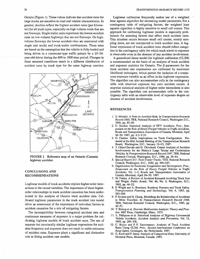
Ontario (Figure 1). These values indicate that accident rates for large trucks are sensitive to road and vehicle characteristics. In general, doubles reflect the highest accident rates (per kilome­ter) for all truck types, especially on high-volume roads that are not freeways. Single trailer units experience the lowest accident rates on low-volume highways that are not freeways. On high­volume freeways the lowest accident rates are associated with single unit trucks and truck-trailer combinations. These rates are based on the assumption that the vehicle is fully loaded and being driven in a commuter-type traffic pattern by a 25-54-year-old driver during the 600 to 1800 time period. Changes in these assumed conditions result in a different distribution of accident rates by truck type for the same highway corridor.

LAKE ONTARIO

FIGURE 1 Reference map of an Ontario (Canada) highway corridor.

CONCLUSIONS AND RECOMMENDATIONS

Loglinear models of truck accidents explore higher-order inter­actions in the causal variables. The importance of these higher­order relationships in truck accident causation has been under­scored in this analysis of Ontario truck accident data. Cal­ibrated loglinear parameters in the truck accident rate model allow an assessment of the importance of individual factors in accident causation for a mix of mitigating factors.

The incompatibility between categorical accident data and continuous measures of exposure is a major problem for cal­ibrating loglinear models of truck accident rates. The use of separate but structurally similar loglinear expressions for acci­dent frequency and exposure does not result in stable estimates of accident rates. Exposure plays a significant and distinctive role in fitting accident rate models.

TRANSPORTATION RESEARCH RECORD 1172

Loglinear calibration frequently makes use of a weighted least squares algorithm for estimating model parameters. For a contingency table of mitigating factors, the weighted least squares algorithm is highly sensitive to small cell counts. This approach for calibrating loglinear models is especially prob­lematic for assessing factors that affect truck accident rates. This situation occurs because small cell counts, mostly sam­pling zeros, are not unexpected in truck accident data. A log­linear expression of truck accident rates should reflect catego­ries in the contingency table for which truck travel or exposure is observable even in the absence of any accident involvement.

A generalized linear model for loglinear calibration (GLIM) is recommended on the basis of an analysis of truck accident and exposure statistics for Ontario. The 13 parameters for the truck accident rate expressions are calibrated by maximum likelihood techniques, which permit the inclusion of a contin­uous exposure variable as an offset in the loglinear expression. The algorithm can also accommodate cells in the contingency table with observed exposure but zero accident counts. A stepwise statistical analysis of higher-order interactions is also possible. The algorithm can accommodate cells in the con­tingency table with an observable level of exposure despite an absence of accident involvement.

REFERENCES

1. D. Mahalel. A Note on Accident Risk. ln Transportation Research Record 1068, TRB, National Research Council, Washington D.C., 1986, pp. 85-89.

2. U. Stocker. Statistical Analysis of HFV Accidents. Proc., Sym­posium on the Role of Heavy Freight Vehicles in Traffic Accidents, Roads and Transportation Association of Canada, Montreal, April 26-30, 1987, pp. 2-3-2-31.

3. 0. Carsten. Safety Implications on Truck Configuration. Pre­sented at the 66th Annual Meeting of the Transportation Research Board, Washington, D.C., January 12-15, 1987.

4. T. Chira-Chavala and D. Oeveland. Causal Analysis of Accident Involvements for the Nation's Large Trucks and Combination Vehicles. In Transportation Research Record I 047, TRB, National Research Council, Washington, D.C., 1986, pp. 56-64.

5. Special Report 21 I: Twin Trailer Trucks, TRB, National Research Council, Washington, D.C., 1986, pp. 304-347.

6. Organization for Economic Cooperation and Development Proc., Symposium on the Role of Heavy Freight Vehicles in Trqffic Accidents, Vol. 1-3, Roads and Transportation Association of Canada, Montreal, April 26-30, 1987.

7. M. Freitas. A Review of Accident Research Involving Truck Size and Weight. Public Roads, Vol. 46, No. 2, Washington, D.C., 1982, pp. 46-52.

8. P. Wright and A. Burnham Roadway Features and Truck Safety. Transportation Planning and Technology, Vol. 9, 1985, pp. 263-269.

9. P. Jovanis and H. Chang. Modelling the Relationship of Accidents to Miles Travelled. In Transportalion Research Record 1068, TRB, National Research Council, Washington, D.C., 1985, pp. 42-51.

10. Y. Bishop et al. Discrete Multivariale Analysis: Theory and Prac­tice. MIT Press, Cambridge, Mass., 1975.

11. L. Philipson et al. Statistical Analyses of Highway Commercial Vehicle Accidents. Accident Analysis and Prevention, Vol. 13, 1988, pp. 289-306.

12. C. Buyco and F. F. Saccomanno. Analysis of Truck Accident Rates Using GLIM. Proc., Second International Conference on Road Safety, Groningen, the Netherlands, 1987.

13. G. Koch and P. Imrey. Analysis of Categorical Data, University of Montreal Press, Montreal, Canada, 1985.

Saccomanno and B~co

14. R. Baker and J. Nedler. GUM Manual. Royal Statistical Society, Oxford, England, 1978.

15. BMDP Manual. University of California Press, Berkeley, 1985. 16. P. McCullagh and J. Nedler. Generalized Linear Models.

Cambridge University Press, Cambridge, England, 1982. 17. Ontario Commercial Vehicle Survey 1983, Policy Planning

Branch, Ontario Ministry of Transportation and Communications, 1984.

31

18. C. Buyco and F. F. Saccomanno. Factors Affecting Truck Accident Rates in Ontario. Department of Civil Engineering, Universily of Waterloo, Waterloo, Canada, 1987.

Publication of this paper sponsored by Committee on Traffic Records and Accident Analysis.