Forecasting of Air Pollution Potential for a Selected … · Forecasting of Air Pollution Potential for a Selected Region in Malaysia Romina Hayati, Nik Meriam Nik Sulaiman, Brahim

© 2014 IJEDR | Volume 2, Issue 3 | ISSN: 2321-9939

IJEDR1403085 International Journal of Engineering Development and Research (www.ijedr.org) 3338

Forecasting of Air Pollution Potential for a Selected

Region in Malaysia

Romina Hayati, Nik Meriam Nik Sulaiman, Brahim Si Ali Chemical Engineering Department,

University of Malaya, 50603 Kuala Lumpur, Malaysia

_______________________________________________________________________________________________________

Abstract - Air pollution issues remain as the ongoing area of concern for posing considerable danger to health throughout

the world (WHO, 2005). For this reason, air pollution related issues and prevention approaches is an essential area of

study more than ever in developing countries like Malaysia. Experimental air pollution potential forecasting study in

Klang Valley-Malaysia during January to December 2009 is described and analysed. In this study, the effect of wind

speed, rainfall, temperature and stability factor of the lower level of atmosphere on potential of air pollution are evaluated

in which Joukoff and Malet (1982) model is used as an initial model. The above meteorological factors first are used to

calculate meteorological air pollution potential (MPI). After that, MPIs vs meteorological factors are evaluated utilizing

time analysis and linear regression. The results discourage the use of foresaid meteorological factor except for

temperature for forecasting of air pollution potential in Malaysia and regions with the same climate characteristics.

Finally, a model for forecasting air pollution potential considering temperature as the most effective factor for the

application in Malaysia is developed.

Keywords - Air Pollution, Air Pollution potential, Forecasting, Meteorological factors, Time series analysis

________________________________________________________________________________________________________

I. INTRODUCTION

Malaysia is located on the South China Sea in the middle of Southeast Asia and situated between 2 30 N, 112 30 E, i.e. within

150 kilometers north of the Equator. The country is crescent- shaped, starting with Peninsular Malaysia (West Malaysia) and

expands to another area, Sabah and Sarawak (East Malaysia), sited on the island of Borneo. The whole area of Malaysia is about

330,000 square km, and the largest part of it is situated on the island of Borneo. Peninsular Malaysia only involves approximately

40% of the whole area. About half of Malaysia is covered by tropical forests mainly in Sabah and Sarawak. Klang Valley located

in the middle part of the west coast of Peninsular Malaysia is considered as the highly developed and fastest growing region in the

country. As a result of rapid development, an effective and reliable monitoring and controlling air quality system is essential. In

addition to emission discharge limits specified by legislation and emissions reduction actions have to be planned at least one or

two days ahead to enhance the effectiveness of the mitigation actions (Monks, et al. 2009). Several studies have been conducted

in order to develop an appropriate model for predicting the air quality worldwide. However, in Malaysia there is paucity of

research in this field.

II. RELATED WORKS

Several studies as shown in Table 1, have been done in order to develop an appropriate model for predicting the air quality

worldwide. Current literature on this topic for the Malaysian situation is scarse as evident in table below.

Table 1 Background of air pollution forecasting studies in Malaysia

Researcher Research Finding

Sani, 1979

Relation between mixing depth and

wind speed through mixing layer,

on air pollution potential (KL and

PJ).

Small mixing depth could cause high concentration of air pollutants in a

region. Differences and similarities between low latitude and mid-

latitude areas must be considered. More research on air pollution

potential in the tropical climate is required.

Aron, 1983 Correlation between mixing height

and air pollution levels

While statistical models are applied to forecast air pollution levels,

omission to involve mixing height as a possible variable will possibly

not corrupt the value of the model.

Ibrahim, et.

al., 2009

Time series technique which was

applicable for forecasting future air

quality in the east coast states of

Malaysia

Predicted values until 2016 for all states apart from NOx for Hulu Klang

did not go beyond the values accepted by NAAQS and DOE Malaysia.

Prediction Method

Surface meteorological data; Met factors (average daily surface wind speed (m/s), average daily surface temperature (°C),

average daily rainfall (mm) were collected from Malaysia Meteorological Department recorded at 8 am and 8 pm at PJ station

which is located at 3° 5' 0" N / 101° 39' 0" E. Upper air data (radio-sonde data) were gathered via online database of Wyoming

University recorded at 8 am and 8 pm at Sepang, KLIA station latitude of 2.71 degree and longitude of 101.7 degree with the



station elevation of 17 meter. The required upper air data (measured by radio-sonde system) used in this research were the altitude

of 700mbar and 1000mbar layer of the atmosphere. These data were compared to upper air data from Malaysia Meteorological

Department randomly to check the validity of data. For all above data set, the average daily value has been used and no data was

missing for the specified period of time. The air pollution index (API) used in this study was obtained from the Malaysia

Department of Environment (DOE) at 7 am, 11 am and 5 pm at Wilayah Persekutuan, Putrajaya Station located at latitude (2.9177

degrees) 2° 55' 3" North of the Equator and longitude (101.6851 degrees) 101° 41' 6" East of the Prime Meridian on the Map of

Kuala Lumpur. The steps of the work are shown in Figure 1.

Figure 1 The work steps

MPI was calculated using Joukoff and Malet model (1)

(1982) utilizing the foresaid meteorological data to determine the

potential of air pollution during 365 days in the year 2009. Terms used in this model are noted in footnotes and explained in

details in Joukoff and Malet paper (1982).

1

2

3

(1)

III. EXPERIMENTAL ANALYSIS AND DISCUSSION

In order to have a general profile of the overall data series, the summarized quantitative description of monthly extremum and

mean values of the surface meteorological factors, and upper air parameters are presented in Table 2.

1 T; surface temperature (°C) while the ambient air temperature is 25°C

2 V; surface wind speed (m/s).

3 S; vertical stability factor,

, H; the thickness of 700-1000 mbar layer of atmosphere, H is obtained for every day

according to daily upper air data by deducting the height of 700mbar layer from 1000mbar layer. Hd ; same thickness according

to adiabatic lapse rate. According to Holton (2004), Hd assumed to be consistent,

P; pressure at higher level of the atmosphere, Po is the pressure at Z=0 ( sea level) , P is the lower pressure layer of the atmosphere

in this study and equals to 700mbar.

Hθ; the total geographical height of the atmosphere

Geographical height is equal to environmental height because Po is the surface pressure and equals to the maximum layer pressure

in this study (1000mbar). Besides, for computational convenience, the mean surface pressure is often assumed to be equal to 1000

hPa; the maximum pressure at which the air parcel could reach. Therefore, the potential temperature (θ) is assumed to be the

average surface temperature.

R; gas constant for dry air, [R = 287 JK-1

kg-1

]

cp; specific heat of dry air at constant pressure, [cp = 1004 JK-1

kg-1

]

go; gravity at sea level, [go = 9.81ms-2

]



Table 2 Summary of quantitative description of surface and upper air data series

Month min V

(m/s)

ave.V

(m/s)

max V

(m/s)

min RF

(mm)

ave. RF

(mm)

max RF

(mm)

min T

(°C)

ave. T

(°C)

max T

(°C)

min He

(m)

ave. He

(m)

max He

(m)

Jan 0.8 2.03 4.1 0 2.11 22.2 25.1 26.85 28.3 29.5 3034 3132.5

Feb 0.9 1.38 2.1 0 4.93 64.8 25.7 26.87 28.5 3030.5 3046.8 3070

Mar 0.7 1.36 2.3 0 11.38 108.8 24.3 26.61 28.1 2886.5 3047.5 3070

Apr 0.8 1.5 3.1 0 9.49 58 25.4 27.41 28.8 3028.5 3064.5 3114.5

May 1 1.58 2.7 0 3.59 42.8 26.6 28.29 30 3026 3051.5 3064.5

Jun 0.6 1.22 2.2 0 1.23 20.2 27.1 27.94 29 3037 3065.9 3077

Jul 1 1.77 3.2 0 4.66 49.4 25.5 27.57 29 3022.5 3046.1 3082.5

Aug 1 1.57 2.5 0 4.14 44 25.5 27.34 28.7 3049.5 3063.8 3073

Sep 0.8 1.34 2 0 7.46 96 24.4 27.25 28.4 3024.5 3044.8 3057

Oct 0.6 1.3 2.1 0 6.14 61 25.6 27.32 28.4 2996 3057.5 3070

Nov 0.8 1.22 1.8 0 9.08 45 24.1 26.38 27.8 2832 3025.3 3055

Dec 0.9 1.47 2.9 0 5.9 40.2 24.5 26.86 28.6 3023.5 3056.1 3062.5

Note: [V; wind speed, RF; rainfall, T; temperature, He; difference height between 1000mbar and 700mbar]

To evaluate the seasonal variation of selected meteorological factors, API and calculated MPI, identifying the season divisions

was essential. According to MMD, maximum rainfall in Klang Valley located on west coast of Peninsular Malaysia occurs in

October and November while February is the month with least rainfall. Based on this fact, four seasons; two monsoons and two

inter-monsoons, can be considered to evaluate seasonal variation of all factors as follow;

First Inter-monsoon: December-January-February, First Monsoon: March-April-May

Second Inter-monsoon: June-July-August, Second Monsoon: September-October-November

Variation of Meteorological Factors

Average monthly and seasonal variation of meteorological factors; wind speed, temperature and rainfall recorded by MMD

during the year 2009 was evaluated by applying the time series analysis method. The results are analyzed and discussed in the

following parts.

Monthly and Seasonal Variation of Temperature

Only slight variation in temperature profile occured throughout the year and maximum variation was less than 6°C (Figure 2).

Minimum surface temperature occurred during the first inter- monsoon through December to February, while in the second inter-

monsoon from June to August, surface temperature reached the maximum value. Besides, during the first monsoon; March to

May, the surface temperature was higher than the second monsoon (Figure 3)

___________________________

Geographical height is equal to environmental height because Po is the surface pressure and equals to the maximum layer pressure

in this study (1000mbar). Besides, for computational convenience, the mean surface pressure is often assumed to be equal to 1000

hPa; the maximum pressure at which the air parcel could reach. Therefore, the potential temperature (θ) is assumed to be the

average surface temperature.

R; gas constant for dry air, [R = 287 JK-1

kg-1

]

cp; specific heat of dry air at constant pressure, [cp = 1004 JK-1

kg-1

]

go; gravity at sea level, [go = 9.81ms-2

]



Figure 2 Variation of monthly average temperature during the year 2009 in Klang Valley

Figure 3 Seasonal variation of average surface temperature during the year 2009 in Klang Valley

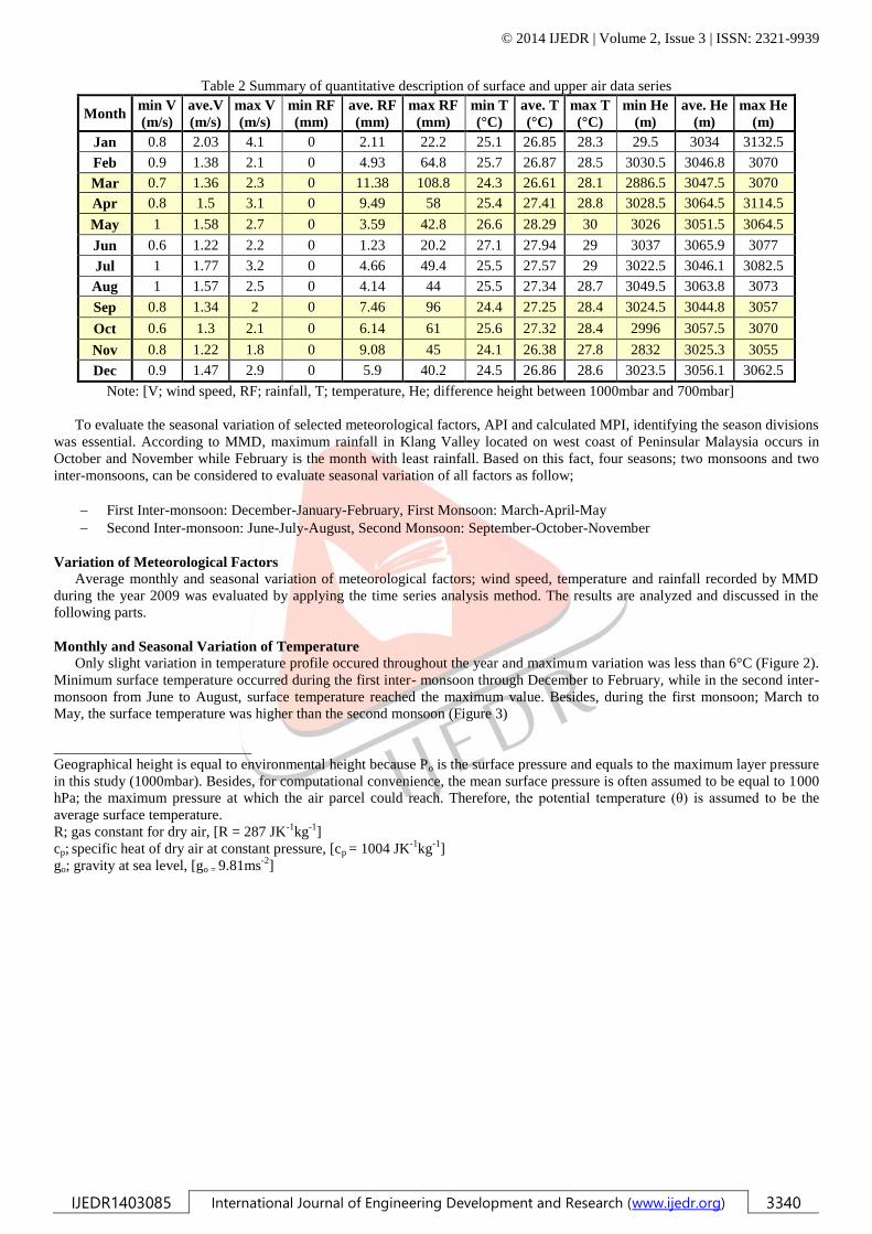
Monthly and Seasonal Variation of Wind Speed

Wind speed was low during the whole year 2009. Maximum average wind speed was recorded to be 2.03m/s in mid

January while minimum recorded value was 1.22m/s in early June (Figure 4). Wind speed in both inter-monsoon periods was

greater than monsoon periods while in first inter-monsoon was greater than the second inter-monsoon. Similarly, wind speed was

greater in the first monsoon compared to the second monsoon (Figure 5).



Figure 4 Variation of monthly average wind speed during the year 2009 in Klang Valley

Figure 5 Variation of seasonal average wind speed during the year 2009 in Klang Valley

Monthly and Seasonal Variation of Rainfall

Maximum average rainfall was 11.38 mm in March while minimum rainfall was 1.23mm in mid June (Figure 6). Maximum

rainfall occurred during March to May (first monsoon) while least rainfall reported during second inter-monsoon. In general, high

quantity of rainfall occurred during two monsoons whereas smallest amount of rainfall happened during inter-monsoon seasons as

usual (Figure 7).



Figure 6 Variation of monthly average rainfall during the year 2009 in Klang Valley

Figure 7 Seasonal variation of rainfall during the year 2009 in Klang Valley

Monthly and Seasonal Variation of Vertical Stability

There was little monthly variation of vertical stability as maximum average vertical stability was 0.85 in mid November while

minimum average values was 0.72 in June, August and April. Therefore, the calculated vertical stability value of the atmosphere

and its variation was very low (about 0.8) (Figure 8). Maximum S occured during the second monsoon through September to

November while minimum S value occurred in second monsoon from June to August (Figure 9).



Figure 8 Variation of monthly average vertical stability during the year 2009 in Klang Valley

Figure 9 Seasonal variation of the average vertical stability during the year 2009 in Klang Valley

Summary of quantitative description of daily calculated vertical stability is presented in Table 3.

Table 3 Summary of quantitative description of daily calculated vertical stability

Month Jan Feb Mar Apr May Jun Jul Aug Sep Oct Nov Dec

min S 0.51 0.7 0.7 0.56 0.72 0.69 0.66 0.69 0.74 0.7 0.75 0.73

ave. S 0.82 0.78 0.78 0.72 0.76 0.72 0.78 0.72 0.78 0.74 0.85 0.75

max S 1.09 0.83 1.32 0.83 0.84 0.81 0.85 0.77 0.85 0.94 1.52 0.85

Monthly and Seasonal Variation of API

Average monthly and seasonal variation of API values obtained by DOE during the year 2009 were evaluated. Figures 10 and

11 show the monthly variation of API during this period. Table 4 shows the mean and extremum monthly values of API during

the year 2009. API value depends on air pollutants concentration through the formulas drived by DOE as it is shown in Table 5.

Table 4 Summary of quantitative description of API




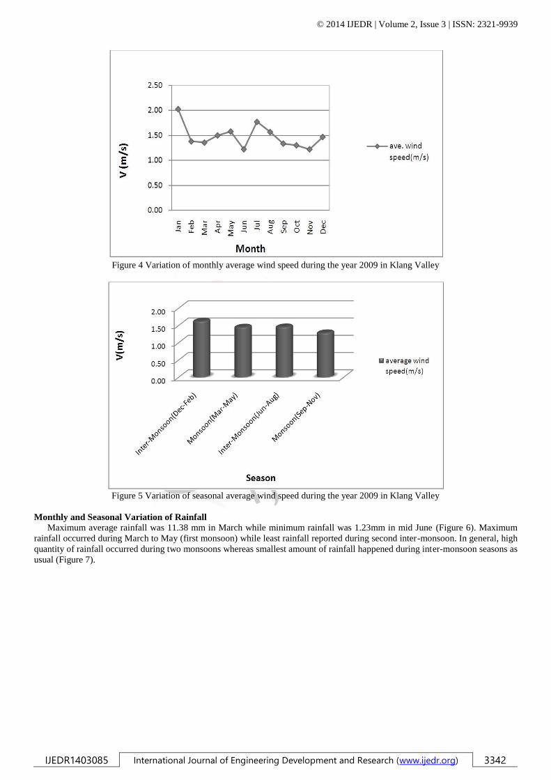
min API 20 20 19 19 29 33 28 20 15 21 16.5 14

ave. API 37 41.7 34.2 36 44.2 52.5 53.8 49 36.8 35.6 25 25.9

max API 56 55 47.5 50 67 91.5 81.5 78.3 66.3 51.5 45 37

Table 5 Calculating API attributing to PM10 and O3 concentration

*C (mg/m3) API **C (ppm)/hr API

C<50 C C<0.2ppm C*1000

50<C<350 50+{[C-50]*0.5} 0.2<C<0.4 200+{[C-0.2]*500}

350<C<420 200+{[C-350]*1.4286} C>0.4 300+{[C-0.4]*1000}

420<C<500 300+{[C-420]*1.25}

C>500 400+[C-500]

*C stands for concentration of PM10

**C stands for concentration of O3

(Source: DOE)

Figure 10 Monthly variation of API during the year 2009 in Klang Valley

Figure 11 Seasonal variation of API value during the year 2009 in Klang Valley

Maximum API values reported during second inter-monsoon from June to August which was quite expected in consequence

of least rainfall because discharge of air pollutants by rainfall was limited and air pollutants could have stayed longer in the

atmosphere at this time. However, two monsoon seasons experienced the lowest values of API as rainfall was maximum because



discharge of pollutants by rainfall increased. In the year 2009 the minimum average value of API was 24.96 which occurred in

November. In mid July API value reaches to the maximum value of 53.72.

Figure 12 Percentage of days with PM10 pollution during the year 2009 in Klang Valley

Figure 13 Percentage of days with PM10 and O3 pollution during the year 2009 in Klang Valley

As presented in Figure 12, in about 346 days of the year 2009, API value was attributed to PM10 concentration; including all

range of concentrations, and it was about 95% of the total days of the year while only 194 days (5%) API values attributed to O3

concentration were verified in the same period in Klang Valley. Percentage of days with PM10 pollution and days with O3

pollution is illustrated in Figure 13.

According to DOE, among different pollutants, the highest concentration of any pollutant is considered as API attributed to

that specific pollutant and among API values for all pollutants, the highest value considered as total API for a day. Based on the

published API by DOE for the year 2009, the number of days with API attributed to the concentration of PM10 and O3 are about

the same as shown in Figure 14.

Figure 14 Rank of PM10 and O3 concentration during the year 2009 in Klang Valley

API value attributed to PM10 less than 50μg/m3 was about 76% (263 out of 346 days). For the rest of the days API value still

was less than 100 as it can be seen from the Figure 15. The total average API which corresponded to either PM10 or O3 is given

in Figure 15 which shows that air quality is in the moderate status and not yet unhealthy. This indicated that the air quality status

in Klang Valley neither exceeded the moderate level defined by DOE API scale nor the Recommended Malaysian Air Quality

Guidelines.



Figure 15 Air quality status during the year 2009 in Klang Valley

Monthly and Seasonal Variation of MPI

Minimum value of average MPI (1.64) occurred in November and in middle of June average MPI reaches to the maximum

value of 3.82 (Figure 16).

Table 6 Summary of quantitative description of MPI


min MPI 0.1 0.77 0.29 0.45 1.53 2.47 0.47 0.47 0.66 0.78 0.1 0.45

ave. MPI 1.66 2.05 1.92 2.8 3.5 3.82 2.56 2.65 2.6 2.77 1.64 2.09

max MPI 3.07 3.83 4.38 4.63 4.57 5.5 4.83 4.73 3.98 3.96 4.17 3.5

Figure 16 Monthly variation of the MPI during the year 2009 in Klang Valley



Figure 17 Seasonal variation of MPI during the year 2009 in Klang Valley

Minimum MPI values occured during first inter-monsoon through December to January. These fluctuations could be as a

direct influence of rainfall and temperature; whenever rainfall amount was high, MPI was low and vice versa. It means that

rainfall and MPI varies conversely during the seasons except for the first inter-monsoon. Moreover, as temperature increased,

MPI also increased proved that temperature and MPI have direct positive correlation (Figure 17).

Monthly Variation of MPI vs. Meteorological Parameters

Monthly variation of MPI values versus each meteorological factor is evaluated in pairs to identify the correlation between

MPI and each of these factors.

MPI vs. Temperature

According to the data and as is shown in Figure 18, temperature variation was small during the year 2009. MPI varied the

same trend as temperature for the whole year. It means that MPI and temperature had a direct correlation; high temperature

resulted in high potential of air pollution and equally low temperature resulted in low potential of air pollution. Civerolo et al.

(1999) shared the same opinion; high temperature would have a tendency to increase emissions.

MPI vs. Wind Speed

MPI varies in the main conversely with wind speed (Figure 19). It means that high wind speed results in low potential of air

pollution; while, the potential of the air pollution is high when wind speed is low. Civerolo et al. (1999), also explained that high

wind velocity would causes enhance pollutant mixing and diffusion however mutual action of temperature and wind velocity

could boost amount of pollutant in some regions and reduce them in some other areas.

Figures 18 Monthly average MPI vs. temperature during the year 2009 in Klang Valley



Figures 19 Monthly average MPI vs. wind speed during the year 2009 in Klang Valley

MPI vs. Rainfall

MPI variation was in opposite path with rainfall variation trend; high rainfall resulted in low potential of air pollution and

potential of air pollution was high when rainfall is small (Figure 20). Seinfeld and Pandis (1998) were on the same opinion that

rainfall play a great role in cleaning the air pollutants.

Since MPI values were small compared to high rainfall amounts, MPI up-scaled (factor of 10) to be comparable with rainfall

values.

MPI vs. Vertical Stability

Vertical stability value was small and varied with mild grade throughout the year 2009 (Figure 21). The value of MPI was also

small; however variation of MPI was greater throughout the year. There was no clear relation between MPI and vertical stability

based on data series and related Figure.

Figures 20 Monthly average MPI vs. rainfall during the year 2009 in Klang Valley



Figures 21 Monthly average MPI vs. vertical stability during the year 2009 in Klang Valley

Monthly and Seasonal Variation of MPI vs. API

Monthly and seasonal variation of calculated MPI and observed API during the year 2009 through January to December was

evaluated. Since computed MPI values were quite small compared to API values, MPI up scaled (factor of 10) to be more tangible

for the purpose of comparing with API. Correlation between these two indexes conducted followed by the regression between

them. The resulted equation then was tested to verify the validation of the equation.

Monthly Variation of MPI vs. API

According to data series for the year 2009 and Figure 22, it is verified that, API values followed the same trend as MPI. It

means that when the potential of air pollution as predicted by MPI was high, it can be expected to have high concentration of air

pollution and attributed API. When potential of air pollution was small, concentration of pollutants could be small logically and

consequently regarded API was low.

Seasonal Variation of MPI vs. API

As it is clear from Figure 23, seasonal variation of MPI was mostly similar with API variation except for the first inter-

monsoon. Maximum MPI values occurred during the second inter-monsoon from Jun to August similar to API values. Minimum

value of MPI occurred during the first inter-monsoon while minimum API reported during second monsoon.

The dissimilarity in the trend for MPI and API values is because MPI is calculated as a function of meteorological factors and

does not related to pollutant concentration directly. Air pollution potential index (MPI) determines the possibility of atmosphere

to keep the pollutants in it whereas air pollution index (API) is obtained based on the observed concentration of pollutants.

Therefore, API and MPI values may not follow the same trend.

Figure 22, Monthly variation of MPI vs. API during the year 2009 in Klang Valley



Figure 23, Seasonal variation of MPI vs. API during the year 2009 in Klang Valley

As explained before in the methodology of the research, MPI model was partially adopted from Joukoff and Malet (1982)

which was conducted in some states in Belgium. Therefore, another reason for dissimilarity between variation paths of MPI and

API most probably is due to big differences between climate and geography of Klang Valley region and the studied areas in

Belgium.

Correlation between API and MPI

According to data series for the year 2009, API values followed the same trend as MPI. Therefore, two-tailed Pearson

Correlation was conducted to determine the exact correlation of this pair. As a result, MPI correlated positively with API (P-value

of 0.014); so, correlation between API and MPI was sensible.

Since API and MPI did correlate positively, linear regression technique was conducted to verify an equation determining

linear correlation between API and MPI. For this purpose, API assumed to be dependent variable, and MPI considered as

independent variable. Consequently, R square was about 0.2 and their relation was linear as demonstrated on Figure 24.

Figure 24 Correlation between MPI and API for the year 2009 in Klang Valley

Linear Regression between API and MPI

As explained in part 4.3, about 76% of the time the concentration of PM10 was less than 50μg/m³. According to Table 4.3 for

formulas quantifying API, reported by DOE, the air pollution index (API) equals to the concentration of PM10 when the

concentration of PM10 is less than 50μg/m³. For other range of concentration of PM10 and for all range of concentration of O3,

API obtained by more complex equations and was not within the scope of this study. One of the limitations of this study is due to

complex and nonlinear relation between the concentration of pollutants and attributed API. Consequently, API equivalent to

concentration of PM10 (C) was used for regression with MPI to determine the direct relation between potential of air pollution

and the concentration of air pollutants.

The regression between API and MPI was conducted in order to attribute MPI to a specific concentration of PM10. Joukoff

and Malet (1982) also conducted the regression technique for corresponding MPI to a specific concentration of SO2.

API (CPM10) considered as dependent variable and MPI was assumed to be independent variable. Equation 2 was determined

as a result of the regression between MPI and API attributed to the concentration of PM10.

C (PM10) = 25.8 + 5.4 MPI (2)

In this equation, C stands for the concentration of PM10 (μg/m³) and C=API when the concentration of PM10 is bellow 50 μg/m³.



To verify the Equation 2, time series analysis for API values corresponded to whole concentration ranges of PM10 and API

calculated by this equation (CPM10) was conducted for the data series of the year 2009. Since, API value for each day assumed to

be equal to the concentrations of PM10 less than 50μg/m³; this equation is only satisfactory for some of low concentrations of

PM10 and this is another limitation of this model. Figure 25 represents the time series variation of reported API by DOE and

calculated API (CPM10) by Equation 2. Also, Figure 26 gives the scatter plot of the observed and forecasted values for the API

during the considered year 2009. As it is clear from the scatter plot, observed API and forecasted API were not equivalent.

Likewise, Joukoff and Malet (1982) has employed this comparison for some states of Belgium but he found that the two data

series were very closed.

Even though in 2009, about 76% of the time the concentration of PM10 was less than 50μg/m³; yet, 24% of higher

concentrations caused a big uncertainty and unreliability for the formula. Therefore, corresponding MPI value to a specific

concentration of any pollutant was not applicable. Hence, it has to be used as its definition; the potential of air pollution index.

Besides, it is necessary to establish a scale for MPI to specify a range for forecasted air pollution potential to be understood easily

by authorities to act properly in advance before the air pollution episode take place. This needs to be further studied in future

works.

Figure 25 Daily variation of average API against average concentration of PM10 (µg/m³) for the year 2009 in Klang Valley

Figure 26 Scatter plot of observed API (O) vs. forecasted API (F) for the year 2009 in Klang Valley

Correlation between API and Meteorological Factors

Monthly APIs and their relation with meteorological factors have been evaluated through Bivariate Pearson Correlation in

order to find their correlation. Final result has been shown by figures to have a clearer picture of these correlations.

According to the finding from the Pearson Correlation, API had negative linear correlation with rainfall and R² linear was very

small (0.009). It means API and rainfall did not have a considerable correlation as shown by Figure 27 and there was no an

understandable influence of rainfall quantity on API value. Similar result for vertical stability has been found but with R² linear of



0.038 as shown in Figure 28. It means vertical stability value did not clearly control API value. In the same way, wind speed had

very small linear correlation with API as R² linear was about 1.366E-4. Figure 29 represents this finding. Finally, API and

temperature had more visible positive correlation with R² linear of 0.0177 as represented in Figure 30. It means that surface

temperature was a determinant factor influencing value of API.

Slini et al. (2002) also conducted scatter plots method for several couples of variables to study their bivariate relationships

which evaluates the linear relationship between those factors.

Figure 27 Correlation between API and rainfall for the year 2009 in Klang Valley

Figure 28 Correlation between API and vertical stability for the year 2009 in Klang Valley

Figure 29 Correlation between API value and wind speed for the year 2009 in Klang Valley



Figure 30 Correlation between API value and surface temperature for the year 2009 in Klang Valley

Correlation between MPI and Meteorological Factors

Monthly MPI and its relation with the meteorological factors have been evaluated through Bivariate Pearson Correlation

technique in order to find each pair correlation. Thus the influence of each factor on MPI value is verified. The result of this

evaluation has been illustrated through Figures in order to have a comprehensible picture of each pair correlations. Figures 31 to

34 represent the linear correlation of MPI with rainfall, vertical stability, wind speed and temperature, respectively.

Figure 31 Correlation between MPI and rainfall throughout the year 2009 in Klang Valley

Figure 32 Correlation between MPI and vertical stability of the atmosphere throughout the year 2009 in Klang Valley



As a result from Pearson Correlation for the data series of the year 2009 in Klang Valley; MPI and rainfall had negative

correlation with R² linear of 0.091 which confirms that rainfall does not correlate strongly with MPI. Likewise MPI and vertical

stability had negative correlation with R² linear of 0.201 which is insignificant correlation. Similarly, MPI and wind speed had

negative correlation with R² linear of 0.014 which is negligible correlation. In contrast, MPI had positive significant linear

relation with temperature with R² linear of 0.815 which is quite meaningful. It indicates that temperature is a key factor in

determining the potential of air pollution.

Figure 33 Correlation between MPI and wind speed during the year 2009 in Klang Valley

Figure 34 Correlation between MPI and temperature throughout the year 2009 in Klang Valley

Since MPI did correlate remarkably with temperature, linear regression technique was employed to find a logical relation

between MPI and temperature resulted in Equation 3.

MPI reg = -25.57 + 1.03 T (3)

Reliability of the equation was evaluated and the result was satisfactory. Figure 35 signifies this finding. It proves that in

Malaysia as a tropical country, the weight of temperature in determining the air pollution potential is significant compared to

vertical stability and wind speed. Figure 36 gives the scatter plot of calculated MPI using meteorological factors and forecasted

MPIreg using regression with surface temperature for the data series of the year 2009 for Klang Valley. Slini et al. (2002) also

utalized a model based on linear regression in order to forecaste the daily air pollution with the help of meteorological and air

quality parameters.



Figure 35 Time series analysis for calculated MPI using meteorological factor vs. MPI reg determined by regression with

temperature throughout the year 2009 in Klang Valley

Figure 36 Scatter plot of MPI and MPIreg for the data series of the year 2009 for Klang Valley

IV. RESULTS AND FINDINGS

Correlation conducted between Malaysia air pollution index (API) and meteorological factors; wind speed, rainfall,

temperature and calculated vertical stability showed that temperature had greatest correlation with API compared to other factors.

Similarly, the result of Bivariate Pearson Correlation between MPI and aforesaid parameters, showed that correlation between

temperature and MPI was the most significant one while there was no clear correlation between MPI with other examined

meteorological factors. Thus, temperature confirmed to be the key factor influencing both API and MPI. Accordingly, the

empirical air pollution potential index (MPIreg) using the linear regression technique was estimated in this study. This index

proved to be more suitable for Malaysia regarding climate and geography compared to the model used by Joukoff and

Malet(1982) for Belgium and the general assessment of the new model (MPIreg) confirmed the problems appearing in statistical

modelling. The low forecasting ability of the model was not unexpected, since a random element in the regression is always there

and remains undetermined. The MPIreg model is assumed to be improved in future studies, as the intention of the current study

was to indicate the effectiveness of temperature for developing an air pollution potential forecasting model. The study also aimed

to show the inefficiency of the other examined meteorological factors; wind speed, rainfall and vertical stability of the

atmosphere, for predicting the potential of air pollution in Malaysia and probably in the regions with similar characteristics.

Moreover, it is the initial stage in this field and is not still a competent model to be used by Malaysian authorities in order to

forecast the air pollution potential. Further studies are required in order to develop a more accurate model for Malaysia.

The study also showed that MPI relatively follows the same trend as API; however, there is no defined range determining

high, moderate or low potential of air pollution. Therefore, it is not easy to use that as a measure for forecasting air pollution

potential.



Linear regression between MPI and API attributed to the concentration of PM10 conducted assuming low concentration of

PM10. Since we need to forecast the high concentration of air pollution or air pollution episode, the exmined model (MPI) is

suggested to be partially suitable as it is not applicable to the whole range of pollutan concentarations.

Eventhough in 2009, the concentration of PM10 about 76% of the time was less than 50μg/m³; yet 24% of higher

concentrations make a big uncertainty and unreliability for MPI formula. Therefore, corresponding MPI value to a specific

concentration of any pollutant is not applicable.

Since the correlation between temperature and MPI was significant, linear regression between temperature and calculated MPI

was conducted and resulted in MPIreg. This MPIreg is probably a more reliable model to be used and implemented for predicting

the air pollution potential. The MPIreg only takes into accout the atmosphere ability to disperse pollutants and does not consider

the sources of pollutants just like MPI.

The current study also showed that, the MPI model developed by Joukoff and Malet (1982) for Belgium does not suit

Malaysia to forecast air pollution potential. According to the data sets for the year 2009 for Klang Valley, by the consideration of

low wind speed, vertical stability and their little variation, these factors are not key parameters regarding to forecasting the

potential of air pollution. Besides, variation of temperature was small as well as small difference between 25°C (ambient air

temperature) and surface temperature (T) compared to the Belgium case. As a result, MPI value for Malaysia was small which

was not so easy to compare with other factors and to have a defined range; high to low potential of air pollution.

This study faced several limitations as follows:

A complex and nonlinear relation between the concentration of pollutants and attributed APIs; therefore, MPIs could not

be attributed to any specific concentration of either O3 or PM10 as the two most concerned pollutants in Malaysia.

Since, API value for each day is assumed to be equal to the concentrations of PM10 less than 50μg/m³, this equation is

mostly satisfactory for low concentrations of PM10.

The data series was collected for one year only because of the budget limitation, which causes uncertainties for the

model to be used as a new approach.

V. CONCLUSION

Experimental air pollution potential forecasting study in Klang Valley-Malaysia during January to December 2009 was

described and analysed. In this study, the effect of wind speed, rainfall, temperature and stability factor of the lower level of

atmosphere on potential of air pollution were evaluated in which Joukoff and Malet (1982) model was used as an initial model.

The above meteorological factors first were used to calculate meteorological air pollution potential (MPI). After that, MPIs vs

meteorological factors are evaluated utalizing time analysis and linear regression. The result discouraged the use of foresaid

meteorological factor exept for temperature for forecasting of air pollution potential in Malaysia and regions with the same

climate characteristics. A model (MPIreg) for forecasting air pollution potential considering most effective factor for the

application in Malaysia was developed. According to the current study, meteorological base model for Malaysia and probably for

the regions with similar climate and geography is different with the models used for temperate countries.

VI. FUTURE WORKS

Since this study showed that temperature was the most determinant factors affecting air pollution potential compared to other

meteorological factors; wind speed, rainfall and vertical stability in Malaysia; therefore, it is suggested that, temperature and

probably relative humidity; which was not evaluated within this research, are effective factors to be used for either improving the

suggested model (MPIreg) or developing a new model for forecasting air pollution potential in Malaysia and regions with similar

characteristics. In addition, it is necessary to establish a scale for MPIreg to specify a range for forecasting air pollution potential to

be understood easily by authorities. Accordingly, authorities could act properly and effectively in advance of the incidence of air

pollution.

Finally, uncertainty can be reduced by using data for longer period of time in order to find scientific and highly precise results.

REFERENCES

[1] Afroz, R., Hassan, M. N., & Ibrahim, N. A. (2003). Review of air pollution and health impacts in Malaysia. Environmental

research, 92(2), 71-77.

[2] Aron, R. (1983). Mixing height--an inconsistent indicator of potential air pollution concentrations. Atmospheric Environment

(1967), 17(11), 2193-2197. doi: Doi: 10.1016/0004-6981(83)90215-9

[3] Baklanov, A., Hänninen, O., Slørdal, L., Kukkonen, J., Bjergene, N., Fay, B., . . . Karppinen, A. (2007). Integrated systems

for forecasting urban meteorology, air pollution and population exposure. Atmospheric Chemistry and Physics, 7(3), 855-

874.

[4] Box, G. E. P., Jenkins, G. M., & Reinsel, G. C. (1976). Time series analysis: forecasting and control (Vol. 16): Holden-day

San Francisco.

[5] Carmichael, G. R., Sandu, A., Chai, T., Daescu, D. N., Constantinescu, E. M., & Tang, Y. (2008). Predicting air quality:

Improvements through advanced methods to integrate models and measurements. Journal of Computational Physics, 227(7),

3540-3571. doi: DOI: 10.1016/j.jcp.2007.02.024

[6] Civerolo, K. L., Sistla, G., Rao, S. T., & Nowak, D. J. (2000). The effects of land use in meteorological modeling:

implications for assessment of future air quality scenarios. Atmospheric Environment, 34(10), 1615-1621. doi: Doi:

10.1016/s1352-2310(99)00393-3



[7] DOE (2010) Air Pollutant Index (API), Ministry of Natural Resources and Environment, Malaysia

[8] DOE (2009) Environmental Air Quality Report, Air Quality Status,Department of Environment-Malaysia

[9] DOE (2009) Malaysia environmental quality report 2009. Ministry of Natural Resources and Environment, Malaysia

[10] DOE (2010) Recommended Malaysian Air Quality Guidelines, Air Quality Trend, Ministry of Natural Resources and

Environment, Malaysia

[11] (EEA, 2007) Atmospheric composition change – global and regional air quality

[12] EPA (1999) Air and Radiation, National Ambient Air Quality Standards (NAAQS)

[13] EPA (2010) Six Common Air Pollutants. U.S. Environmental Protection Agency, USA

[14] Field, A. P. (2009). Discovering statistics using SPSS: SAGE publications Ltd.

[15] Gao, J., & Zha, Y. (2010). Meteorological Influence on Predicting Air Pollution from MODIS-Derived Aerosol Optical

Thickness: A Case Study in Nanjing, China. Remote Sensing, 2(9), 2136-2147.

[16] Goyal, P., & Rama Krishna, T. V. B. P. S. (2002). Dispersion of pollutants in convective low wind: a case study of Delhi.

Atmospheric Environment, 36(12), 2071-2079. doi: Doi: 10.1016/s1352-2310(01)00458-7

[17] Holton, J. R. (2004). An introduction to dynamic meteorology: Academic press.

[18] Hrust, L., Klaic, Z. B., Krizan, J., Antonic, O., & Hercog, P. (2009). Neural network forecasting of air pollutants hourly

concentrations using optimised temporal averages of meteorological variables and pollutant concentrations. Atmospheric

Environment, 43(35), 5588-5596. doi: DOI: 10.1016/j.atmosenv.2009.07.048

[19] Ibrahim, M. Z., Zailan, R., Ismail, M., & Lola, M. S. (2009). Forecasting and time series analysis of air pollutants in several

area of Malaysia. American Journal of Environmental Sciences, 5(5), 625-632.

[20] Joukoff, A., & Malet, L. (1982). Daily forecasting of air pollution potential. Science of The Total Environment, 23, 97-102.

[21] Kurt, A., & Oktay, A. B. (2010). Forecasting air pollutant indicator levels with geographic models 3 days in advance using

neural networks. Expert Systems with Applications, 37(12), 7986-7992.

[22] MMD (2011) General Climate of Malaysia, Ministry of Sience, Technology and Innovation(MOSTI), Malaysia

Meteorological Department

[23] Monks, P., Granier, C., Fuzzi, S., Stohl, A., Williams, M., Akimoto, H., . . . Bey, I. (2009). Atmospheric composition change-

global and regional air quality. Atmospheric Environment, 43(33), 5268-5350.

[24] Motulsky, H. (1995). Intuitive biostatistics (Vol. 173): Oxford University Press New York.

[25] Peng, C. L. (2007). Environmental Threat in Malaysia, from http://scienceray.com/biology/ecology/environmental-threats-in-

malaysia/

[26] Sani, S. (1990). Urban climatology in Malaysia: An overview. Energy and Buildings, 15(1-2), 105-117. doi: Doi:

10.1016/0378-7788(90)90121-x

[27] Sarji, A. H. A. (1993). Malaysia's vision 2020: understanding the concept, implications, and challenges: Pelanduk

Publications.

[28] Seaman, N. L. (2000). Meteorological modeling for air-quality assessments. Atmospheric Environment, 34(12-14), 2231-

2259. doi: Doi: 10.1016/s1352-2310(99)00466-5

[29] Seinfeld, J. H., & Pandis, S. N. (1998). Atmospheric chemistry and physics: from air pollution to climate change (Vol. 1).

[30] Slini, T., Karatzas, K., & Papadopoulos, A. (2002). Regression analysis and urban air quality forecasting: An application for

the city of Athens. Global NEST, 4(2-3), 153-162.

[31] Thiessen, A. H. (1946). Weather glossary: US Dept. of Commerce, Weather Bureau.

[32] Trochim, W. M. K. (2006, 20.10.2006). research methods knowledge base, from

http://www.socialresearchmethods.net/kb/statdesc.php

[33] WHO (2010) Air Quality in Asia, Status and Trends, Edition 2010, World Health Organization

[34] WHO (2008) Air Quality and Health, World Health Organization

[35] WHO ( 2005) Public Health and Environment (PHE), Air quality guidelines - global update 2005

http://scienceray.com/biology/ecology/environmental-threats-in-malaysia/

http://scienceray.com/biology/ecology/environmental-threats-in-malaysia/

http://www.socialresearchmethods.net/kb/statdesc.php

Documents

Forecasting of Air Pollution Potential for a Selected … · Forecasting of Air Pollution Potential for a Selected Region in Malaysia Romina Hayati, Nik Meriam Nik Sulaiman, Brahim