Embed Size (px)
Citation preview

1
I hereby declare that, except where specifically indicated,
the work submitted herein is my own original work.
Date: _____________ Signature: _____________
Finite Element Studies on the Mechanical Stability of Arbitrarily
Oriented and Inclined Wellbores Using a Vertical 3D Wellbore Model
by Di Zien Low (F)
Fourth-Year Undergraduate Project in Group D, 2010/2011

2
LIST OF CONTENTS
PART 1: TECHNICAL ABSTRACT .................................................................................................. 5
PART 2: INTRODUCTION ........................................................................................................... 7
2.1 Definition of Wellbore Stability ....................................................................... 8
2.2 Factors Affecting Wellbore Stability ............................................................... 8
2.3 Past Works on Developing Wellbore Stability Models ................................... 11
2.4 Computational Finite-Element Analysis .......................................................... 12
2.5 Aims of Project ................................................................................................. 13
PART 3: THEORY AND DESIGN OF EXPERIMENT ............................................................................ 14
3.1 Elastic Stress Transformation for and Arbitrarily Oriented Borehole ............. 14
3.2 Stresses and Strains in Cylindrical Coordinate ................................................ 15
3.3 General Elastic Solution for a Borehole in Cylindrical Coordinate .................. 15
3.4 Wellbore Inclination in Planes Perpendicular to and ......................... 17
3.5 Finite-Element Wellbore Models Considered ................................................. 19
3.6 Dimensions, Meshes and Elements of the Wellbore Model .......................... 21
PART 4: EXPERIMENTAL TECHNIQUES AND PROCEDURES ............................................................... 23
4.1 Experimental Data and Local In-Situ Stress Calculations ................................ 24
4.2 The Geostatic Stage ......................................................................................... 29
4.3 Important ABAQUS Keywords ......................................................................... 30
4.4 The Drilling Stage ............................................................................................ 32
4.5 Data Extraction and Analysis ........................................................................... 34
PART 5: RESULTS AND DISCUSSION ............................................................................................ 35
5.1 Comparing Mathematical and ABAQUS Models under Isotropic Loads ......... 38
5.2 Comparison of Results with Data Published by Zhou et al (1996) .................. 45
PART 6: CONCLUSION .............................................................................................................. 47
PART 7: FUTURE WORKS ......................................................................................................... 47
PART 8: REFERENCES ............................................................................................................... 48
PART 9: APPENDIX .................................................................................................................. 50

3
LIST OF FIGURES
2.1 Borehole Breakout Schematic ................................................................................... 7
3.1 In-Situ Coordinate System ......................................................................................... 14
3.2 Coordinate System for Deviated Borehole ............................................................... 14
3.3 Borehole Orientation and Coordinates ..................................................................... 14
3.4 Local Borehole Stresses and Strains in Cylindrical Coordinate System .................... 15
3.5 Plane Stress Transformation Equations .................................................................... 17
3.6 Mohr’s Circle of Stress for Plane Stress Transformation .......................................... 18
3.7 Symmetrical Quarter-Vertical Wellbore Model ........................................................ 19
3.8 Symmetrical Half-Vertical Wellbore Model .............................................................. 19
3.9 Full-Inclined Wellbore Model .................................................................................... 20
3.10 Dimensions of the Symmetrical Half-Vertical Wellbore Model ................................ 21
3.11 Mesh and Elements of the Symmetrical Half-Vertical Wellbore Model ................... 21
3.12 Partition around the Wellbore .................................................................................. 22
3.13 Mesh around the Wellbore ....................................................................................... 22
3.14 20-Node C3D20RP Element Type .............................................................................. 22
4.1 Inclination Plane for Case #A and Case #B ................................................................ 25
4.2 Boundary Conditions at the Geostatic Stage ............................................................ 29
4.3 Loads at the Geostatic Stage ..................................................................................... 30
4.4 Cylindrical Coordinate System .................................................................................. 30
4.5 Drilling Fluid Pressure Supports the Borehole Wall in the Drilling Stage ................. 33
4.6 Pore Pressure Applied to Back and Side Surfaces, Others Assumed Impermeable .. 33
4.7 Circumferential Stress Contours of Case 4B (β=60°) at the end of Drilling Stage .... 34
5.1 Case 1A – Mathematical Model ................................................................................ 36
5.2 Case 1A – ABAQUS Model ......................................................................................... 37
5.3 Case 2A – ABAQUS Model ......................................................................................... 39
5.4 Case 2B – ABAQUS Model ......................................................................................... 40
5.5 Case 3A – ABAQUS Model ......................................................................................... 41
5.6 Case 3B – ABAQUS Model ......................................................................................... 42
5.7 Case 4A – ABAQUS Model ......................................................................................... 43
5.8 Case 4B – ABAQUS Model ......................................................................................... 44
5.9 Chart Produced by Zhou et al (1996) ........................................................................ 45

4
LIST OF TABLES
4.1 Well Data for All Cases (1A, 2A, 2B, 3A, 3B, 4A and 4B) ........................................... 24
4.2 Far Field Total and Effective Stresses ........................................................................ 24
4.3 Rock Type and Properties ......................................................................................... 25
4.4 Stresses Applied to ABAQUS Model at Various Well Inclinations for Case 1A ......... 25
4.5 Stresses Applied to ABAQUS Model at Various Well Inclinations for Case 2A ......... 26
4.6 Stresses Applied to ABAQUS Model at Various Well Inclinations for Case 2B ......... 26
4.7 Stresses Applied to ABAQUS Model at Various Well Inclinations for Case 3A ......... 27
4.8 Stresses Applied to ABAQUS Model at Various Well Inclinations for Case 3B ......... 27
4.9 Stresses Applied to ABAQUS Model at Various Well Inclinations for Case 4A ......... 28
4.10 Stresses Applied to ABAQUS Model at Various Well Inclinations for Case 4B ......... 28
5.1 Result Figures and Loading Cases ............................................................................. 35

5
PART 1: TECHNICAL ABSTRACT
This study aims to define a comprehensive method that can transform a vertical wellbore
model into any arbitrarily oriented wellbore model, which can then be used repeatedly to
analyse the stability and stress distribution around wellbores at any orientation. The finite –
element software package ABAQUS will be used to create the symmetrical half-vertical
wellbore finite-element model, which will then be used to analyse the stability and stress
distribution around wellbores inclined at in planes perpendicular to the far
field minimum and maximum principal stresses where = 0° and = 90°.
The staged approach will be implemented by first bringing the normal and shear stresses as
well as pore pressure acting on the block of soil into equilibrium at the Geostatic Stage; a
cylindrical borehole will then be removed from the block of soil using model change at the
Drilling Stage. Soil properties such as density, elasticity, friction angle, cohesion, dilation,
void ratio and pore pressure will be applied to the 3D finite-element wellbore model. The
wellbore model will then be transformed and inclined in two different azimuth planes, one
perpendicular to the far-field maximum horizontal stress, and the other perpendicular to
the far-field minimum horizontal stress. The effects of isotropic and increasing anisotropic
far-field horizontal stresses on the wellbore stability and stress distribution around wellbore
will also be examined at constant far-field overburden stress.
The mathematical model published by Jaeger and Cook (1979) for an arbitrarily oriented
wellbore in an isotropic linear elastic material and the research findings of Zhou et al (1996),
which suggested that inclined wellbores can be more stable than a vertical well in an
extensional stress regime, will be used to verify that the methods proposed in this study to
transform a vertical finite-element model into any arbitrarily oriented and inclined wellbore
by changing the normal and shear stress applied to the model is acceptable and justifiable.
If this research proves to be successful, it may translate into major time savings in future
works of wellbore stability analysis as vertical wellbore models are easier to build, partition,
mesh, debug and analyse compared to inclined wellbore models. Besides that, there will be
no need to create countless finite-element models with wellbores set at different angles to
analyse the stress distribution around wellbores at a various inclination and orientation,
only one comprehensive vertical wellbore model will be required to test everything.

6
This study intends to prove the following hypotheses:
1. Appropriate sets of normal and shear stresses can be applied to the surfaces of a 3D
finite-element vertical wellbore model to transform it into an inclined wellbore model;
2. By applying different sets of normal and shear stresses, the same vertical wellbore model
can be reused and transformed into wellbores at different inclination and orientation;
3. The wellbore stability and stress distribution around an arbitrarily oriented and inclined
wellbore can be analysed using a single 3D finite-element vertical wellbore model.
The steps below highlight the experimental procedures taken in this study:
Step 1: Identify the magnitudes of the far-field principal stresses
Step 2: Determine the azimuth (α) and inclination (β) angles required for the test
Step 3: Calculate local in-situ normal and shear stresses base on required α and β
Step 4: Build the 3D finite-element vertical wellbore model using ABAQUS
Step 5: Apply material properties, boundary conditions to the wellbore model
Step 6: Referring to the stresses calculated in Step 3, apply loads to the model
Step 7: Run Geostatic Stage, check that stresses are in equilibrium and displacement is zero
- If failed, return to Steps 4, 5, 6 and 7 to debug the problem, repeat until OK
Step 8: Run Drilling Stage, remove borehole using ‘Model Change’ and apply mud pressure
- If failed, return to Steps 4, 5, 6, 7 and 8 to debug the problem, repeat until OK
Step 9: Extract Data from the nodes around the wellbore using Field Output Requests
Step 10: Repeat Steps 2 – 9 to analyse wellbores at different azimuth (α) and inclination (β)
The results show that the mathematical theory published by Jaeger and Cook (1979) and
finite-element result agrees that a vertical wellbore is most stable under isotropic horizontal
stress. Under the same loading, both analysis also agree with each other that maximum
stress anisotropy occurs at β = 90°, i.e. when the wellbore is horizontal. Besides that, the
result published by Zhou et al (1996) agrees quite well with the results obtained in this study.
For starters, vertical wellbores will always be the most stable under isotropic conditions.
Then, as the stress horizontal stress anisotropy increases, the value of increases as well,
which then increases the required inclination angle to give the most stable wellbore. Overall,
the hypotheses were proven to be successful, but more work can still be done by creating a
full vertical wellbore model to test the wellbore transformation in other azimuth planes.

7
PART 2: INTRODUCTION
The stability of a wellbore is one of the major issues surrounding drilling operations. It is the
main cause of non-productive time during drilling operations and costs the oil and gas
industry worldwide more than USD 6 billion annually.1
Before a well is drilled, subsurface rocks are under well-balanced stress conditions with the
three in-situ principal stresses: vertical, horizontal maximum and horizontal maximum,
which also produce shear stresses on planes within the rock mass. 2 However, this
equilibrium state will change when cylindrical sections of rocks are removed at the drilling
stages and replaced by drilling fluids at specific mud weights to provide temporary support.
If the wellbore is not supported, the rock formation around the wellbore might become
unstable and collapse. According to Kang et al (2009), drilling fluid can only partially support
the normal stresses on the wellbore wall but not the shear stresses, as the original rock does,
and this result in stress concentration and redistribution around the wellbore.
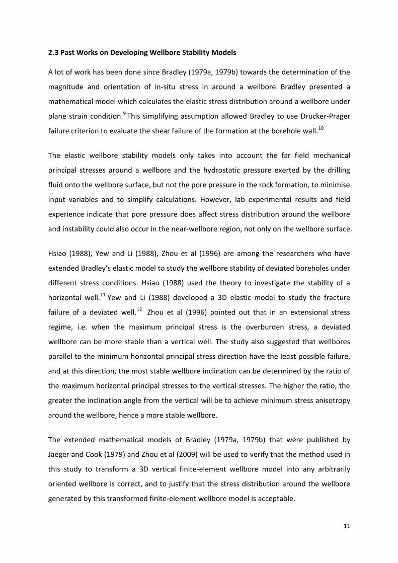
In such cases, rock failures or “breakouts” will
occur at the fractured zones of the borehole
wall where the tangent of the circular borehole
is parallel to the direction of the maximum
horizontal stress3, as shown in Figure 2.1. The
greater the stress anisotropy between the
maximum and minimum horizontal stresses, the
more serious the breakouts will be. These rock
deformations redistribute the stress around the
borehole until a new equilibrium is achieved.
Wellbores can be drilled vertically, inclined, or horizontally (i.e. 90° inclination) and it has
been widely recognised that highly deviated, extended-reach and horizontal wells can offer
economic benefits through lower development costs, faster production rates, and higher
recovery factors.4 Since the mid-20th century, the use of controlled directional drilling
technology has increased dramatically to reach otherwise inaccessible reserves.5 However,
inclined and horizontal wells may be prone to mechanical instability in high in-situ stresses. 6
Figure 2.1: Borehole Breakout Schematic3

8
2.1 Definition of Wellbore Stability
According to Kang et al (2009), a wellbore is considered to be stable when its diameter
equals to the drill-bit diameter and remains the same shape for an extended period of time.
Besides that, Kang et al (2009) also stated that wellbore instability can be considered as a
function of how rocks respond to the induced stress concentration around the wellbore
during various drilling activities. However, the general understanding is that as long as the
borehole surface remains intact and does not collapse during and after drilling operations,
the wellbore can be considered as stable.
On the other hand, Zhou et al (1996) suggested the concept of minimum stress anisotropy
around a wellbore when the research group tries to identify the optimum drilling direction
and inclination angle under various magnitudes of far-field principal stresses. This concept
appears to be more appropriate and will be adopted in this study to assess the stability of
wellbores across various orientations. Hence, the definition of a stable wellbore will be one
that has the minimum stress anisotropy around its borehole surface.
2.2 Factors Affecting Wellbore Stability2
Wellbore instability is a very complicated phenomenon as various factors can affect the
stress distribution around the wellbore. Many wellbore stability models were presented in
the past to address the wellbore stability issue. Most of the existing models examine one or
a combination of two or more of the following effects on wellbore stability: mechanical,
hydraulic, chemical, and thermal. A comprehensive study regarding the major factors
affecting wellbore stability has been done by Kang et al (2009) and is summarised as follow:
(a) Rock Mechanical Properties
Rock mechanical properties such as Young’s modulus, Poisson’s ratio, Biot’s constant,
rock porosity, permeability, bulk density, cohesive strength, tensile strength, and
internal friction etc. are among the parameters that can affect borehole behaviour.
Although rock properties cannot be controlled by drilling engineers, a good knowledge
of the rock mechanical properties can help well planners predict the stability of a
wellbore and minimise risk by choosing a suitable well path before drilling.

9
(b) Far-field Principal Stresses
The in-situ principal stresses are calculated from the three far-field principal stresses:
overburden stress, maximum horizontal stress and minimum horizontal stress. For
wellbore stability analysis, the overburden stress is relatively easy to get from density
logs, but a lot of work needs to be done to determine the magnitude and direction of
the maximum and minimum horizontal stresses in the field. It has been observed in the
field that wellbores deform differently under different horizontal stress conditions. This
clearly shows that good understanding of the magnitude and direction of far-field
principal stresses are important to analyse the stability of a wellbore.
(c) Wellbore Trajectory
In order to transform the far-field principal stresses into the in-situ stresses around a
wellbore, the azimuth and inclination angle of a wellbore are required. Normal and
shear stresses acting on the rock formation in the near-wellbore region are functions of
the azimuth and inclination, and this will be discussed in detail in Part 3 of this report.
Unlike rock properties and far-field principal stresses, wellbore trajectory is something
that can be determined by the drilling engineer. Careful design of wellbore trajectory
during well planning may help to avoid any borehole failure in the drilling operations.7
(d) Pore Pressure
Based on the effective stress concept, stresses acting on the rock formation in the near-
wellbore region are partially supported by the pore pressure within the rock formation.
Any changes in the pore pressure can affect the stress state around the wellbore. Hence,
accurate pore pressure prediction is important in wellbore stability analysis as well.
(e) Mud Weight
Drilling fluids within specific mud weights are used to provide temporary support to the
borehole walls in drilling operations. Drilling fluids need to be heavy enough to support
the borehole and prevent it from collapsing. A common practice in the field to maintain
wellbore stability is by increasing the mud weight. However, the mud weight must not
be too high as heavy drilling fluid may exert too much hydrostatic pressure on the
borehole wall and cause the rock formation to fracture.

10
(f) Drilling Fluid and Pore Fluid Chemicals
Due to the different composition and concentration of chemicals in the drilling fluid and
pore fluid, a chemical potential difference can be generated between these two fluids
while drilling through rock formation. Such chemical potential difference can cause fluid
to flow in or out of the pores and result in pore pressure redistribution. The effects due
to chemical potential difference can be neglected for highly permeable formations such
as sandstone, but is a major concern for low permeability formations such as shale. This
is because the induced fluid flow can generate significant pore pressure propagation
and redistribution in low permeability formations. This is also one of the reasons why
the drilling fluid composition and concentration are closely monitored and controlled in
the field to prevent shale formations from failure.
(g) Temperature
As drilling operations extend to deep wells, temperature differences of about 60°C to
70°C between the circulated drilling fluid and the rock formation can result in tens of
MPa of thermally induced stresses in the rock formation.8 In addition to the thermally
induced stresses, temperature can also change the chemical potential in the drilling
fluid and pore fluid, resulting in transient fluid flow in the near-wellbore region.
(h) Time
Chemical and thermal effects can cause pore pressure propagation in the rock
formation and thus redistributes the stresses around the wellbore over a period of time.
Hence, wellbore stability is also time-dependent phenomenon.
This study intends to incorporate wellbore stability factors (a) to (e) into a 3D finite-element
wellbore model subjected to isotropic and anisotropic far-field principal stresses to examine
local in-situ stress distribution around the wellbore. Vertical overburdened stress and mud
weight will remain constant and the in-situ stresses around the wellbore will be observed at
various inclination angles in two azimuth planes. The computational result will then be
compared to the mathematical model published by Jaeger and Cook (1979) for an arbitrarily
oriented borehole, which assumes plane strain condition normal to the borehole axis, as
well as by Zhou et al (2009), to gain better understanding about wellbores stability issues.
11
2.3 Past Works on Developing Wellbore Stability Models
A lot of work has been done since Bradley (1979a, 1979b) towards the determination of the
magnitude and orientation of in-situ stress in around a wellbore. Bradley presented a
mathematical model which calculates the elastic stress distribution around a wellbore under
plane strain condition.9 This simplifying assumption allowed Bradley to use Drucker-Prager
failure criterion to evaluate the shear failure of the formation at the borehole wall.10
The elastic wellbore stability models only takes into account the far field mechanical
principal stresses around a wellbore and the hydrostatic pressure exerted by the drilling
fluid onto the wellbore surface, but not the pore pressure in the rock formation, to minimise
input variables and to simplify calculations. However, lab experimental results and field
experience indicate that pore pressure does affect stress distribution around the wellbore
and instability could also occur in the near-wellbore region, not only on the wellbore surface.
Hsiao (1988), Yew and Li (1988), Zhou et al (1996) are among the researchers who have
extended Bradley’s elastic model to study the wellbore stability of deviated boreholes under
different stress conditions. Hsiao (1988) used the theory to investigate the stability of a
horizontal well.11 Yew and Li (1988) developed a 3D elastic model to study the fracture
failure of a deviated well.12 Zhou et al (1996) pointed out that in an extensional stress
regime, i.e. when the maximum principal stress is the overburden stress, a deviated
wellbore can be more stable than a vertical well. The study also suggested that wellbores
parallel to the minimum horizontal principal stress direction have the least possible failure,
and at this direction, the most stable wellbore inclination can be determined by the ratio of
the maximum horizontal principal stresses to the vertical stresses. The higher the ratio, the
greater the inclination angle from the vertical will be to achieve minimum stress anisotropy
around the wellbore, hence a more stable wellbore.
The extended mathematical models of Bradley (1979a, 1979b) that were published by
Jaeger and Cook (1979) and Zhou et al (2009) will be used to verify that the method used in
this study to transform a 3D vertical finite-element wellbore model into any arbitrarily
oriented wellbore is correct, and to justify that the stress distribution around the wellbore
generated by this transformed finite-element wellbore model is acceptable.

12
2.4 Computational Finite-Elements Analysis
With the increase in computational power, development of sophisticated software and the
reduction in costs, the extensive use of computational techniques such as finite-element
methods to model wellbore stability has increased in recent years. The latest finite-element
software packages allow one to combine the mathematical theories of solid mechanics such
as elasticity, plasticity, poroelasticity and viscoelasticity, with different failure theories and
wellbore components to create more realistic and sophisticated models.13
The finite-element model may exhibit linear or non-linear behaviour and can still be tested
and calibrated using experimental data to give realistic visual representation and analysis
about what is actually happening around the wellbore. The ability of finite-element software
to generate stress contours and displacement plots at incremental time frames throughout
the drilling operation allows the computational analysis to be pieced together to create a
continuous video, which can then be used to provide better ‘feel’ and insights into how and
why the wellbore actually deforms, which may otherwise be impossible.
Over the past ten years, with the rapid development of robust non-linear finite-element
method techniques that are suitable to analyse complex geomechanics, soil mechanics and
rock mechanics, the finite-element software package ABAQUS (SIMULIA)14 has successfully
been used to perform finite-element analysis to analyse horizontal-casing integrity15,
cement sheath integrity16, sand production17, hydraulic fracturing18 and many more.
While some researchers prefer to concentrate on analysing the stress state at a particular
stage of life-of well without considering the previous loading and deformation history, Gray
et al (2007) suggested that the staged approach should be used and stated that, “The staged
approach imitates construction of the well, following all or some of the development stages
such as drilling, casing, cementing, completion, hydraulic fracturing, and production. By use
of the finite-element method, the stress state at each stage is modelled, and stage variables
such as the amount of damage and plasticity along with loading and boundary conditions
are transmitted to the model for the next stage. This technique eliminates the need to guess
the initial state of stress, amount of plasticity and damage.” This study will use and adapt
the staged approach proposed by Gray et al (2009) to analyse the stability of a wellbore.

13
2.5 Aims of Project
This study will focus on creating a vertical wellbore model using the ABAQUS finite-element
software package, and then establishing a comprehensive method to transform this vertical
model into any arbitrary oriented and inclined wellbore model. This allows the same vertical
wellbore model to be used repeatedly to examine the stability and stress distribution
around wellbores at any orientation by changing the magnitude and direction of local in-situ
normal and shear stress acting on the vertical wellbore model only.
The staged approach will be implemented by first bringing the normal and shear stresses as
well as pore pressure acting on the block of soil into equilibrium at the Geostatic Stage; a
cylindrical borehole will then be removed from the block of soil using model change at the
Drilling Stage. Soil properties such as density, elasticity, friction angle, cohesion, dilation,
void ratio and pore pressure will be applied to the 3D finite-element wellbore model. The
wellbore model will be transformed and inclined in two different azimuth planes, one
perpendicular to the far-field maximum horizontal stress, and the other perpendicular to
the far-field minimum horizontal stress. The effects of isotropic and increasing anisotropic
far-field horizontal stresses on the wellbore stability and stress distribution around wellbore
will also be examined at constant far-field overburden stress.
The mathematical model published by Jaeger and Cook (1979) for an arbitrarily oriented
wellbore in an isotropic linear elastic material and the research findings of Zhou et al (1996),
which suggested that inclined wellbores can be more stable than a vertical well in an
extensional stress regime, will be used to verify that the methods proposed in this study to
transform a vertical finite-element model into any arbitrarily oriented and inclined wellbore
by changing the normal and shear stress applied to the model is acceptable and justifiable.
If this research proves to be successful, it may translate into major time savings in future
works of wellbore stability analysis as vertical wellbore models are easier to build, partition,
mesh, debug and analyse compared to inclined wellbore models. Besides that, there will be
no need to create countless finite-element models with wellbores set at different angles to
analyse the stress distribution around wellbores at a various inclination and orientation,
only one comprehensive vertical wellbore model will be required to test everything.
14
PART 3: THEORY AND DESIGN OF EXPERIMENT
3.1 Elastic Stress Transformation for an Arbitrarily Oriented Borehole19,20
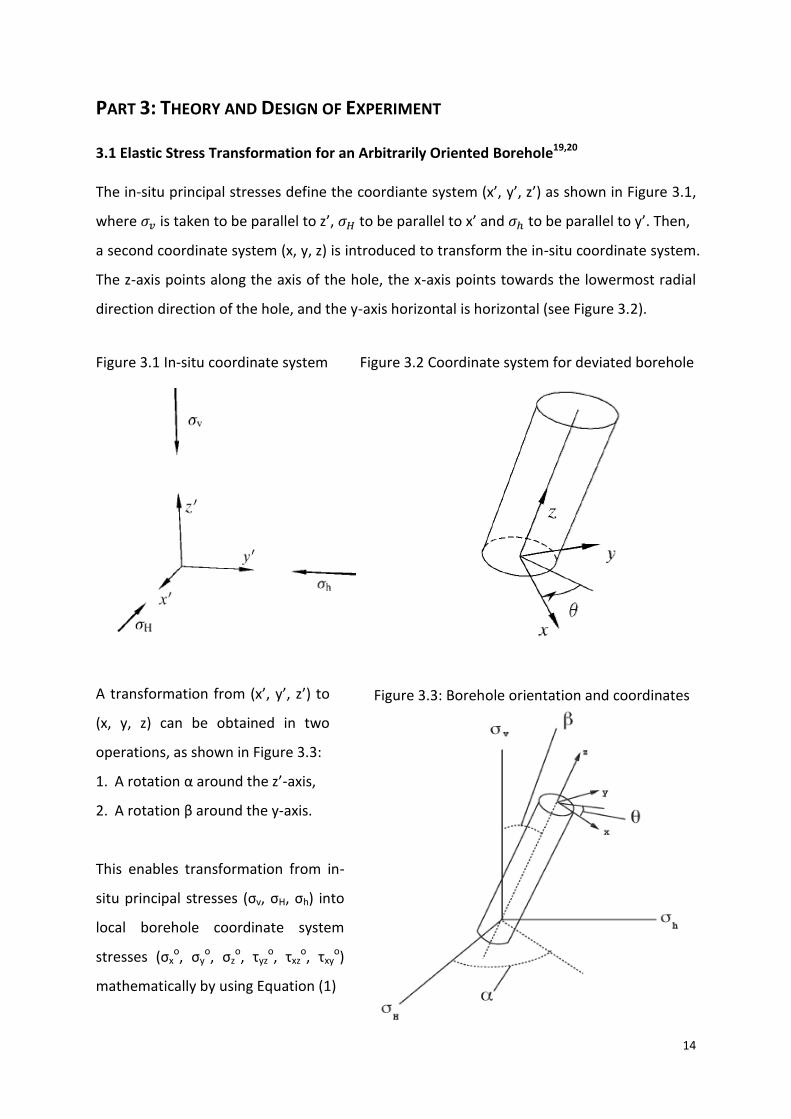
The in-situ principal stresses define the coordiante system (x’, y’, z’) as shown in Figure 3.1,
where is taken to be parallel to z’, to be parallel to x’ and to be parallel to y’. Then,
a second coordinate system (x, y, z) is introduced to transform the in-situ coordinate system.
The z-axis points along the axis of the hole, the x-axis points towards the lowermost radial
direction direction of the hole, and the y-axis horizontal is horizontal (see Figure 3.2).
Figure 3.1 In-situ coordinate system Figure 3.2 Coordinate system for deviated borehole
A transformation from (x’, y’, z’) to
(x, y, z) can be obtained in two
operations, as shown in Figure 3.3:
1. A rotation α around the z’-axis,
2. A rotation β around the y-axis.
This enables transformation from in-
situ principal stresses (σv, σH, σh) into
local borehole coordinate system
stresses (σxo, σy
o, σzo, τyz
o, τxzo, τxy
o)
mathematically by using Equation (1)
Figure 3.3: Borehole orientation and coordinates

15
According to Jaeger and Cook (1979), for an arbitrarily oriented borehole shown in Figure3.3,
the rotation of the stress tensor from the global in-situ coordinate system (σv, σH, σh) to a
local borehole Cartesian coordinate system (σxo, σy
o, σzo, τyz
o, τxzo, τxy
o) is given by
{
}
{
}
{
} .......(1)
Note: Superscript o on the stresses denote that these are virgin formation stresses.
3.2 Stresses and Strains in Cylindrical Coordinate
To examine the stresses and strains in the rock
surrounding a borehole, it will be convenient to
express the local borehole Cartesian coordinates
system derived from the in-situ principal stresses
in Equation (1) into local cylindrical coordinates
(r, θ, z). The cylindrical coordinate stresses and
strains at a point in a plane perpendicular to the
z-axis are shown in Figure 3.4
3.3 General Elastic Solution for a Borehole in Cylindrical Coordinate (Fjaer et al, 2008)
Assuming plane strain normal to the borehole axis in the local cylindrical coordinates (r, θ, z)
where r represents the distance from the borehole axis, θ the azimuth angle relative to the
x-axis, and z is the position along the borehole axis, for an arbitrary borehole with radius Rw,
excess fluid pressure pw acting on the surface of the borehole wall, and formation Poisson’s
ratio vfr, the general elastic solution for (σr, σθ, σz, τrθ, τθz, τrz) can be written as follow4:
(
)
(
)
(
)
.............(2)
Figure 3.4: Local Borehole Stresses and
Strains in Cylindrical Coordinate System
r

16
(
)
(
) (
)
.....(3)
* (
)
+ .............(4)
(
) (
) .............(5)
(
) (
) ............................................................(6)
(
) (
) ............................................................(7)
The borehole influence is given by the terms in and , which vanish rapidly with
increasing radial distance from the borehole axis . The general elastic solutions depend on
angle , indicating that the stresses vary with position around the wellbore. Generally, the
shear stresses are non-zero. Thus , and are not principal stresses for arbitrary
orientations of the well. At the borehole surface ( = ), the equations can be simplified to:
...............................................................................(8)
(
) ............................................(9)
(
)
......................................... (10)
............................................................................ (11)
(
) ............................................................................ (12)
............................................................................ (13)
where
= in-situ effective vertical principal stress
= in-situ effective major horizontal principal stress
= in-situ effective minor horizontal principal stress
= Poisson’s ratio of the formation
= angle between and the projection of the borehole axis onto the horizontal plane
= angle between the borehole axis and the vertical direction
= polar angle in the borehole cylindrical coordinate system
= excess fluid pressure in the borehole = mud pressure less pore pressure in formation
= stress tensor in the local borehole Cartesian coordinate system
= stress tensor in the local borehole cylindrical coordinate system

17
3.4 Wellbore Inclination in Planes Perpendicular to and
Special conditions exist when the wellbore rotates in planes perpendicular to the far-field
minimum principal axis at = 0° and in planes perpendicular to the far-field maximum
principal axis at = 90°. The following equations are derived from Equation (1).
At = 0° and for any inclination angle β
{
}
{
}
{
} .................... (14)
At = 90° and for any inclination angle β
{
}
{
}
{
} ........... (15)
This analysis shows that when the wellbore is inclined in the planes perpendicular to the far-
field minimum and maximum principal axis at = 0° and = 90°, the local in-situ shear
stress that acts on the wellbore model only exist in the X-Z plane, i.e. within the same plane
where the wellbore is inclined. Shear stresses in the X-Y and Y-Z plane will be zero. This may
be useful when it comes to identifying a suitable finite-element model for this study.
Figure 3.5: Plane Stress Transformation Equations
σy σ
τyz
τxy
Quick Check:
𝜎𝑦 𝜎𝐻
𝜏𝑦𝑧
𝜏𝑥𝑦
Quick Check:
β
’
’ β
18
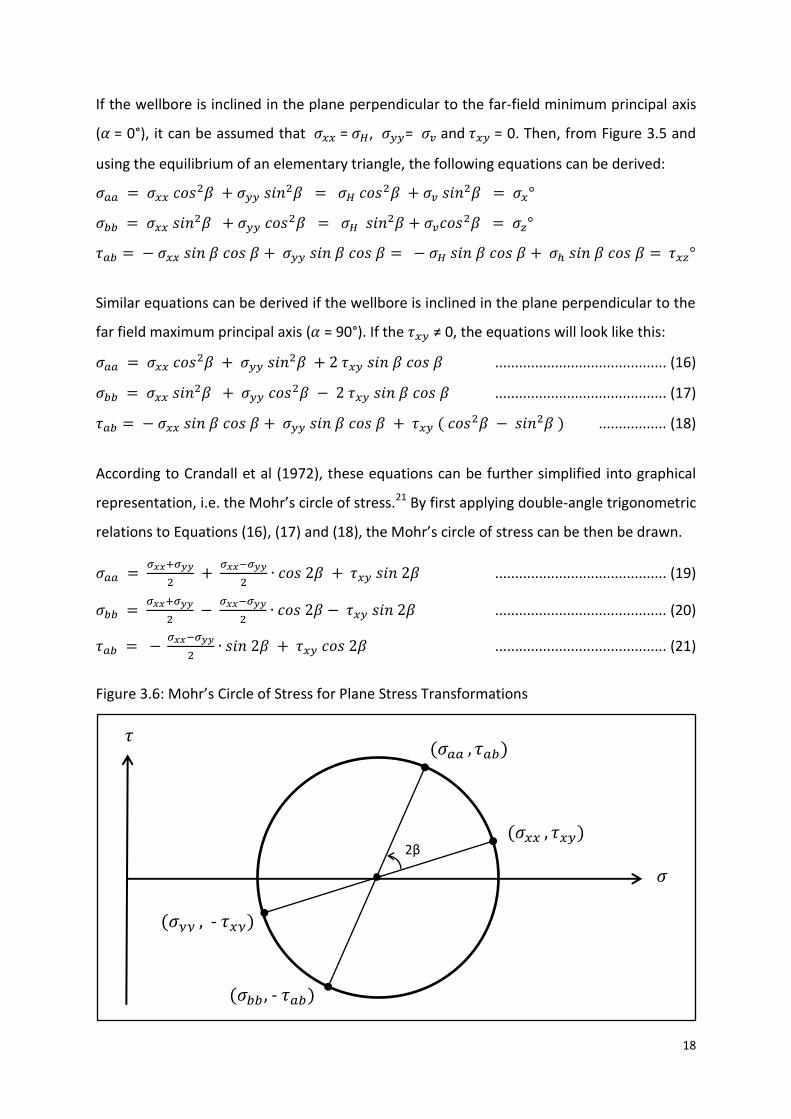
If the wellbore is inclined in the plane perpendicular to the far-field minimum principal axis
( = 0°), it can be assumed that = , = and = 0. Then, from Figure 3.5 and
using the equilibrium of an elementary triangle, the following equations can be derived:
Similar equations can be derived if the wellbore is inclined in the plane perpendicular to the
far field maximum principal axis ( = 90°). If the ≠ 0, the equations will look like this:
........................................... (16)
........................................... (17)
................. (18)
According to Crandall et al (1972), these equations can be further simplified into graphical
representation, i.e. the Mohr’s circle of stress.21 By first applying double-angle trigonometric
relations to Equations (16), (17) and (18), the Mohr’s circle of stress can be then be drawn.
........................................... (19)
........................................... (20)
........................................... (21)
Figure 3.6: Mohr’s Circle of Stress for Plane Stress Transformations
𝜎𝑎𝑎 𝜏𝑎𝑏
𝜎𝑏𝑏 - 𝜏𝑎𝑏
𝜎
𝜏
2β 𝜎𝑥𝑥 𝜏𝑥𝑦
𝜎𝑦𝑦 - 𝜏𝑥𝑦

19
3.5 Finite-Element Wellbore Models Considered
Figure 3.7: Symmetrical Quarter-Vertical Wellbore Model
In this study, shear stress needs to be
applied to the surfaces of the model to
create an inclined wellbore. However,
the symmetrical quarter-vertical model
faces complications as shear stress do
not form complete loops around the
model. This model is only suitable to
analyse vertical or horizontal wellbores
that is perpendicular to , and .
Figure 3.8: Symmetrical Half-Vertical Wellbore Model
The half-vertical wellbore model allows
shear stress to a make complete loop
around the X-Z plane, i.e. the vertical
wellbore can be rotated in the X-Z plane.
However, the model is limited to rotate
perpendicularly to or as these are
the only directions where shear stress
around X-Y and Y-Z plane are zero.
Otherwise, a full model will be required.
Full-Vertical Wellbore Model
This combines two symmetrical half-vertical wellbore model to create a block of soil with a
cylindrical vertical wellbore drilled through the middle. The full vertical wellbore model,
allows the wellbore model to be transformed into any orientation and inclination as shear
stresses can form complete loops around any of the X-Y, X-Z and Y-Z planes, without the
shear stress symmetrical issues that exist for the quarter and half vertical wellbore models.
However, a full vertical wellbore model contains twice as many element as the half model.
This means that a lot more resources, time and computing power is required to run the
finite-element analysis, which are the main things that this research study seriously lack of.

20
Figure 3.9: Full-Inclined Wellbore Model
The full-inclined wellbore model is an alternative to analyse the wellbore stability of an
arbitrarily oriented and inclined wellbore. No stress transformation calculation will be
required for this model as the far-field stress that acts normally to the block surfaces and
the cylindrical wellbore that has been carefully created at a specific angle will do the job.
It must be recognised that an inclined wellbore can only analyse wellbore stability and stress
distribution around a wellbore at one inclination only. A lot of inclined wellbore models may
need to be created if various analyses at different orientation and inclination are required.
Hence, it is fair to say that inclined wellbore models are not as reusable as vertical wellbore
models that make use stress transformations. Also, because local in-situ normal and shear
stresses can be calculated from the far-field principal stresses base on the desired azimuth
and inclination angles, and these local in-situ normal and shear stresses can then be applied
easily to the surfaces of the same vertical wellbore model by simple change of numbers to
create any desired orientation and inclination, only one comprehensive vertical wellbore
model that has been properly built and thoroughly checked will be required.
As one of the aims of this study is to establish a comprehensive method that can transform
a vertical wellbore model into any arbitrary oriented and inclined wellbore model, as well as
considering the limited resources, time and computing power, the symmetrical half-vertical
wellbore finite-element model will be used to analyse the stability and stress distribution
around wellbores inclined at in rotational planes perpendicular to and .

21
3.6 Dimensions, Meshes and Elements of the Wellbore Model
Figure 3.10: Dimensions of the Symmetrical Half-Vertical Wellbore Model
Figure 3.11: Mesh and Elements of the Symmetrical Half-Vertical Wellbore Model
2m
1m
1m
0.5m
0.5m
0.5m
0.5m
0.5m
0.5m
R1
R2
R3

22
Figure 3.12: Partition around the Wellbore Figure 3.13: Mesh around the Wellbore
#
Two additional concentric cylindrical partitions will be made to facilitate the convergence of
mesh lines towards the centreline of the borehole, as well as to ensure that the number and
size the elements can be controlled more effectively throughout the wellbore model.
Element type C3D20RP will be assigned to and used in the entire
wellbore model. According to the ABAQUS Analysis User’s Manual,
each C3D20RP element is a 20-node brick that analyse triquadratic
displacements, trilinear pore pressures, with reduced integration.
This will do the job of analysing pore pressures, stresses and
displacements in the model. The model will be 10 element-layers
thick and have finer elements around the vicinity of the borehole.
There will be 20 elements per 180° arc of the borehole and the overall layout of the mesh
and relative size of the elements can be found in Figures 3.11 and 3.16. A rough calculation
suggests that the wellbore model will have a total of 6280 elements and 28721 nodes.
The soil parameters for the model, the displacement and pore pressure boundary conditions,
and the direction and magnitude of the stresses that needs to be applied on which surface
of the wellbore model and at what stage will be discussed in detail in the next section.
R1 = 0.06m
R2 = 0.12065m
R3 = 0.35m
Borehole Boundary
Borehole Boundary
Figure 3.14: 20-Node
C3D20RP Element Type

23
PART 4: EXPERIMENTAL TECHNIQUES AND PROCEDURES
As discussed earlier, this study aims to define a comprehensive method that can transform a
vertical wellbore model into any arbitrarily oriented wellbore model, which can then be
used repeatedly to analyse the stability and stress distribution around wellbores at any
orientation. With the considerations of limited resources, time and computing power, the
symmetrical half-vertical wellbore finite-element model will be used to analyse the stability
and stress distribution around wellbores inclined at in planes perpendicular
to the far field minimum and maximum principal stresses where = 0° and = 90°.
This study intends to prove the following hypotheses:
4. Appropriate sets of normal and shear stresses can be applied to the surfaces of a 3D
finite-element vertical wellbore model to transform it into an inclined wellbore model;
5. By applying different sets of normal and shear stresses, the same vertical wellbore model
can be reused and transformed into wellbores at different inclination and orientation;
6. The wellbore stability and stress distribution around an arbitrarily oriented and inclined
wellbore can be analysed using a single 3D finite-element vertical wellbore model.
The steps below highlight the experimental procedures taken in this study:
Step 1: Identify the magnitudes of the far-field principal stresses
Step 2: Determine the azimuth (α) and inclination (β) angles required for the test
Step 3: Calculate local in-situ normal and shear stresses base on required α and β
Step 4: Build the 3D finite-element vertical wellbore model using ABAQUS
Step 5: Apply material properties, boundary conditions to the wellbore model
Step 6: Referring to the stresses calculated in Step 3, apply loads to the model
Step 7: Run Geostatic Stage, check that stresses are in equilibrium and displacement is zero
- If failed, return to Steps 4, 5, 6 and 7 to debug the problem, repeat until OK
Step 8: Run Drilling Stage, remove borehole using ‘Model Change’ and apply mud pressure
- If failed, return to Steps 4, 5, 6, 7 and 8 to debug the problem, repeat until OK
Step 9: Extract Data from the nodes around the wellbore using Field Output Requests
Step 10: Repeat Steps 2 – 9 to analyse wellbores at different azimuth (α) and inclination (β)

24
4.1 Experimental Data and Local In-Situ Stress Calculations
The example problem published by Gray et al (2007) will be used and adapted in this study
Table 4.1 - Well Data for All Cases (1A, 2A, 2B, 3A, 3B, 4A and 4B)
True Vertical Depth of the Well 15000 ft. 4572 m
Estimated Hole Diameter Being Drilled 9.5 inch 0.2413 m
Overburden Pressure Gradient 1 psi/ft. 22.62 kPa/m
Pore Pressure Gradient 0.62 psi/ft. 14.0248 kPa/m
Table 4.2 - Far-Field Total and Effective Stresses
Case 1A 2A, 2B 3A, 3B 4A, 4B Unit
Total Vertical Stress, 103421 103421 103421 103421 kPa
Total Horizontal Maximum Stress, 92437 94775 95885 99332 kPa
Total Horizontal Minimum Stress, 92437 90099 88990 85542 kPa
Pore Pressure, 64121 64121 64121 64121 kPa
Effective Vertical Stress, 39300 39300 39300 39300 kPa
Effective Horizontal Maximum Stress, 28316 30654 31763 35211 kPa
Effective Horizontal Minimum Stress, 28316 25978 24869 21421 kPa
Difference Between Effective Horz Stress, 0 4676 6894 13790 kPa
K1 = / = 0.72 0.78 0.81 0.90 -
K2 = / 1.00 1.18 1.28 1.64 -
K3 = / = 0.72 0.66 0.63 0.55 -
Average Effective Horz Stress, ( ) / 2 28316 28316 28316 28316 kPa
All cases have the same vertical and average horizontal stresses
Case 1A: Isotropic Horizontal Stresses, well inclination β in α = 0° azimuth plane only
Case 2A: Anisotropic Horizontal Stresses, well inclination β in α = 0° azimuth plane
Case 2B: Anisotropic Horizontal Stresses, well inclination β in α = 90° azimuth plane
Case 3A: Larger Anisotropic Horizontal Stresses, well inclination β in α = 0° azimuth plane
Case 3B: Larger Anisotropic Horizontal Stresses, well inclination β in α = 90° azimuth plane
Case 4A: Largest Anisotropic Horizontal Stresses, well inclination in α = 0° azimuth plane
Case 4B: Largest Anisotropic Horizontal Stresses, well inclination in α = 90° azimuth plane

25
Figure 4.1: Inclination Plane for Case #A and Case #B
Table 4.3 - Rock Type and Properties
Rock Type
Young's Modulus,
E (kPa)
Poisson's Ratio, v
Friction Angle, φ (°)
Cohesive Strength,
c (kPa)
Dilation Angle, ψ (°)
Density, ρ
(kg/m3)
Permeability,
k (m/s) Void Ratio
R3c3 2.70E+07 0.2 30 5.93E+07 0.1 2500 1.00E-08 0.33
Table 4.4 – Stresses Applied to ABAQUS Model at Various Well Inclinations for Case 1A
Well inclination, β 0 15 30 45 60 75 90 degree
= C – R cos(2β) 92437 93173 95183 97929 100675 102686 103421 kPa
= 92437 92437 92437 92437 92437 92437 92437 kPa
= C + R cos(2β) 103421 102686 100675 97929 95183 93173 92437 kPa
= R sin(2β) 0 2746 4756 5492 4756 2746 0 kPa
Pore pressure, u 64121 64121 64121 64121 64121 64121 64121 kPa
Effective 28316 29052 31062 33808 36554 38564 39300 kPa
Effective 28316 28316 28316 28316 28316 28316 28316 kPa
Effective 39300 38564 36554 33808 31062 29052 28316 kPa
R = 5492
C = 97929
𝜎𝑣 = 103421 𝜎𝐻 = 92437
𝜎 𝜏
𝜎 - 𝜏
𝜎 𝑘𝑃𝑎
𝜏 𝑘𝑃𝑎
2β
𝜎 𝜎 = 𝜎 𝑡𝑜𝑡𝑎𝑙
𝜎
𝜏
𝜏
𝜎𝑣
𝜎𝐻 𝜎 𝛼 ) 𝛼 )
Inclination
Plane for
Ca e #B
Inclination
Plane for
Ca e #A

26
Table 4.5 – Stresses Applied to ABAQUS Model at Various Well Inclinations for Case 2A
Azimuth Plane, α 0 0 0 0 0 0 0 degree
Well inclination, β 0 15 30 45 60 75 90 degree
= C – R cos(2β) 94775 95355 96937 99098 101260 102842 103421 kPa
= 90099 90099 90099 90099 90099 90099 90099 kPa
= C + R cos(2β) 103421 102842 101260 99098 96937 95355 94775 kPa
= R sin(2β) 0 2162 3744 4323 3744 2162 0 kPa
Pore pressure, u 64121 64121 64121 64121 64121 64121 64121 kPa
Effective 30654 31233 32816 34977 37139 38721 39300 kPa
Effective 25978 25978 25978 25978 25978 25978 25978 kPa
Effective 39300 38721 37139 34977 32816 31233 30654 kPa
Table 4.6 – Stresses Applied to ABAQUS Model at Various Well Inclinations for Case 2B
Azimuth Plane, α 90 90 90 90 90 90 90 degree
Well inclination, β 0 15 30 45 60 75 90 degree
= C – R cos(2β) 90099 90992 93430 96760 100091 102529 103421 kPa
= 94775 94775 94775 94775 94775 94775 94775 kPa
= C + R cos(2β) 103421 102529 100091 96760 93430 90992 90099 kPa
= R sin(2β) 0 3331 5769 6661 5769 3331 0 kPa
Pore pressure, u 64121 64121 64121 64121 64121 64121 64121 kPa
Effective 25978 26870 29309 32639 35970 38408 39300 kPa
Effective 30654 30654 30654 30654 30654 30654 30654 kPa
Effective 39300 38408 35970 32639 29309 26870 25978 kPa
R = 4323
C = 97929
𝜎𝑣 = 103421 𝜎𝐻 = 94775
𝜎 𝜏
𝜎 - 𝜏
𝜎 𝑘𝑃𝑎
𝜏 𝑘𝑃𝑎
2β
R = 6661
C = 96760
𝜎𝑣 = 103421 𝜎 = 90099
𝜎 𝜏
𝜎 - 𝜏
𝜎 𝑘𝑃𝑎
𝜏 𝑘𝑃𝑎
2β
𝜎 𝜎 = 𝜎𝐻 𝑡𝑜𝑡𝑎𝑙
𝜎
𝜏
𝜏
𝜎
𝜎
𝜎 = 𝜎 𝑡𝑜𝑡𝑎𝑙
𝜏
𝜏

27
Table 4.7 – Stresses Applied to ABAQUS Model at Various Well Inclinations for Case 3A
Azimuth Plane, α 0 0 0 0 0 0 0 degree
Well inclination, β 0 15 30 45 60 75 90 degree
= C – R cos(2β) 95885 96390 97769 99653 101537 102916 103421 kPa
= 88990 88990 88990 88990 88990 88990 88990 kPa
= C + R cos(2β) 103421 102916 101537 99653 97769 96390 95885 kPa
= R sin(2β) 0 1884 3263 3768 3263 1884 0 kPa
Pore pressure, u 64121 64121 64121 64121 64121 64121 64121 kPa
Effective 31763 32268 33648 35532 37416 38795 39300 kPa
Effective 24869 24869 24869 24869 24869 24869 24869 kPa
Effective 39300 38795 37416 35532 33648 32268 31763 kPa
Table 4.8 – Stresses Applied to ABAQUS Model at Various Well Inclinations for Case 3B
Azimuth Plane, α 90 90 90 90 90 90 90 degree
Well inclination, β 0 15 30 45 60 75 90 degree
= C – R cos(2β) 88990 89957 92598 96206 99813 102455 103421 kPa
= 95885 95885 95885 95885 95885 95885 95885 kPa
= C + R cos(2β) 103421 102455 99813 96206 92598 89957 88990 kPa
= R sin(2β) 0 3608 6249 7216 6249 3608 0 kPa
Pore pressure, u 64121 64121 64121 64121 64121 64121 64121 kPa
Effective 24869 25835 28477 32084 35692 38333 39300 kPa
Effective 31763 31763 31763 31763 31763 31763 31763 kPa
Effective 39300 38333 35692 32084 28477 25835 24869 kPa
R = 3768
C = 99653
𝜎𝑣 = 103421 𝜎𝐻 = 95885
𝜎 𝜏
𝜎 - 𝜏
𝜎 𝑘𝑃𝑎
𝜏 𝑘𝑃𝑎
2β
R =
C =
𝜎𝑣 = 103421 𝜎 = 88990
𝜎 𝜏
𝜎 - 𝜏
𝜎 𝑘𝑃𝑎
𝜏 𝑘𝑃𝑎
2β
𝜎 𝜎 = 𝜎𝐻 𝑡𝑜𝑡𝑎𝑙
𝜎
𝜏
𝜏
𝜎
𝜎
𝜎 = 𝜎 𝑡𝑜𝑡𝑎𝑙
𝜏
𝜏
28
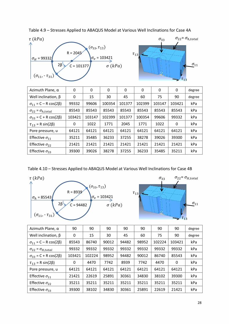
Table 4.9 – Stresses Applied to ABAQUS Model at Various Well Inclinations for Case 4A
Azimuth Plane, α 0 0 0 0 0 0 0 degree
Well inclination, β 0 15 30 45 60 75 90 degree
= C – R cos(2β) 99332 99606 100354 101377 102399 103147 103421 kPa
= 85543 85543 85543 85543 85543 85543 85543 kPa
= C + R cos(2β) 103421 103147 102399 101377 100354 99606 99332 kPa
= R sin(2β) 0 1022 1771 2045 1771 1022 0 kPa
Pore pressure, u 64121 64121 64121 64121 64121 64121 64121 kPa
Effective 35211 35485 36233 37255 38278 39026 39300 kPa
Effective 21421 21421 21421 21421 21421 21421 21421 kPa
Effective 39300 39026 38278 37255 36233 35485 35211 kPa
Table 4.10 – Stresses Applied to ABAQUS Model at Various Well Inclinations for Case 4B
Azimuth Plane, α 90 90 90 90 90 90 90 degree
Well inclination, β 0 15 30 45 60 75 90 degree
= C – R cos(2β) 85543 86740 90012 94482 98952 102224 103421 kPa
= 99332 99332 99332 99332 99332 99332 99332 kPa
= C + R cos(2β) 103421 102224 98952 94482 90012 86740 85543 kPa
= R sin(2β) 0 4470 7742 8939 7742 4470 0 kPa
Pore pressure, u 64121 64121 64121 64121 64121 64121 64121 kPa
Effective 21421 22619 25891 30361 34830 38102 39300 kPa
Effective 35211 35211 35211 35211 35211 35211 35211 kPa
Effective 39300 38102 34830 30361 25891 22619 21421 kPa
R = 2045
C = 101377
𝜎𝑣 = 103421 𝜎𝐻 = 99332
𝜎 𝜏
𝜎 - 𝜏
𝜎 𝑘𝑃𝑎
𝜏 𝑘𝑃𝑎
2β
R = 8939
C = 94482
𝜎𝑣 = 103421 𝜎 = 85543
𝜎 𝜏
𝜎 - 𝜏
𝜎 𝑘𝑃𝑎
𝜏 𝑘𝑃𝑎
2β
𝜎 𝜎 = 𝜎𝐻 𝑡𝑜𝑡𝑎𝑙
𝜎
𝜏
𝜏
𝜎
𝜎
𝜎 = 𝜎 𝑡𝑜𝑡𝑎𝑙
𝜏
𝜏
29
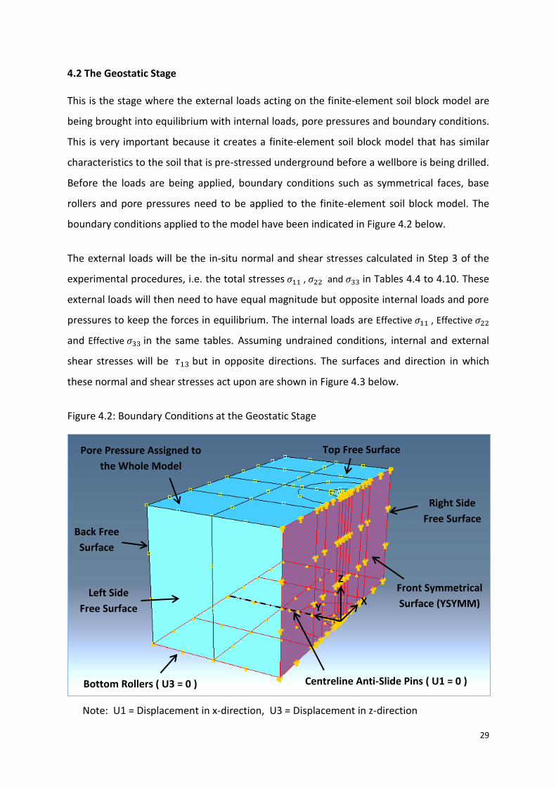
4.2 The Geostatic Stage
This is the stage where the external loads acting on the finite-element soil block model are
being brought into equilibrium with internal loads, pore pressures and boundary conditions.
This is very important because it creates a finite-element soil block model that has similar
characteristics to the soil that is pre-stressed underground before a wellbore is being drilled.
Before the loads are being applied, boundary conditions such as symmetrical faces, base
rollers and pore pressures need to be applied to the finite-element soil block model. The
boundary conditions applied to the model have been indicated in Figure 4.2 below.
The external loads will be the in-situ normal and shear stresses calculated in Step 3 of the
experimental procedures, i.e. the total stresses , and in Tables 4.4 to 4.10. These
external loads will then need to have equal magnitude but opposite internal loads and pore
pressures to keep the forces in equilibrium. The internal loads are Effective , Effective
and Effective in the same tables. Assuming undrained conditions, internal and external
shear stresses will be but in opposite directions. The surfaces and direction in which
these normal and shear stresses act upon are shown in Figure 4.3 below.
Figure 4.2: Boundary Conditions at the Geostatic Stage
Note: U1 = Displacement in x-direction, U3 = Displacement in z-direction
Front Symmetrical
Surface (YSYMM)
Top Free Surface
Bottom Rollers ( U3 = 0 ) Centreline Anti-Slide Pins ( U1 = 0 )
Pore Pressure Assigned to
the Whole Model
Z
X Y
Back Free
Surface
Left Side
Free Surface
Right Side
Free Surface

30
Figure 4.3: Loads at the Geostatic Stage
Note: is being applied perpendicularly onto the back surface of the model
4.3 Important ABAQUS Keywords
The origin (0, 0, 0) will be positioned at the base
of the model with the z-axis placed along the
centreline of the cylindrical borehole. ABAQUS
is capable of transforming Cartesian coordinates
automatically into cylindrical coordinates.
For SYSTEM=CYLINDRICAL, points a and b lie on the polar axis of the cylindrical system. The
local axes are: 1 = radial, 2 = circumferential, 3 = axial. To assign the cylindrical coordinate
system to the model, the following lines into the Parts section of the ABAQUS input file:
* ORIENTATION, NAME=R-THETA, SYSTEM=CYLINDRICAL
0, 0, 0, 0, 0, 1
3, 0
1st Data Line: X-coordinate of point a, Y-coordinate of point a, Z-coordinate of point a,
X-coordinate of point b, Y-coordinate of point b, Z-coordinate of point b
2nd Data Line: Local direction about which additional rotation is given (3 = axial),
Additional rotation defined by a single scalar value. Default = 0.
𝝈𝟏𝟏 𝝈𝟏𝟏
𝝈𝟑𝟑
𝝉𝟏𝟑
𝝉𝟏𝟑
𝝉𝟏𝟑
𝝉𝟏𝟑
Top, Right
Bottom, Left
Z
X
Figure 4.4: Cylindrical Coordinate System
31
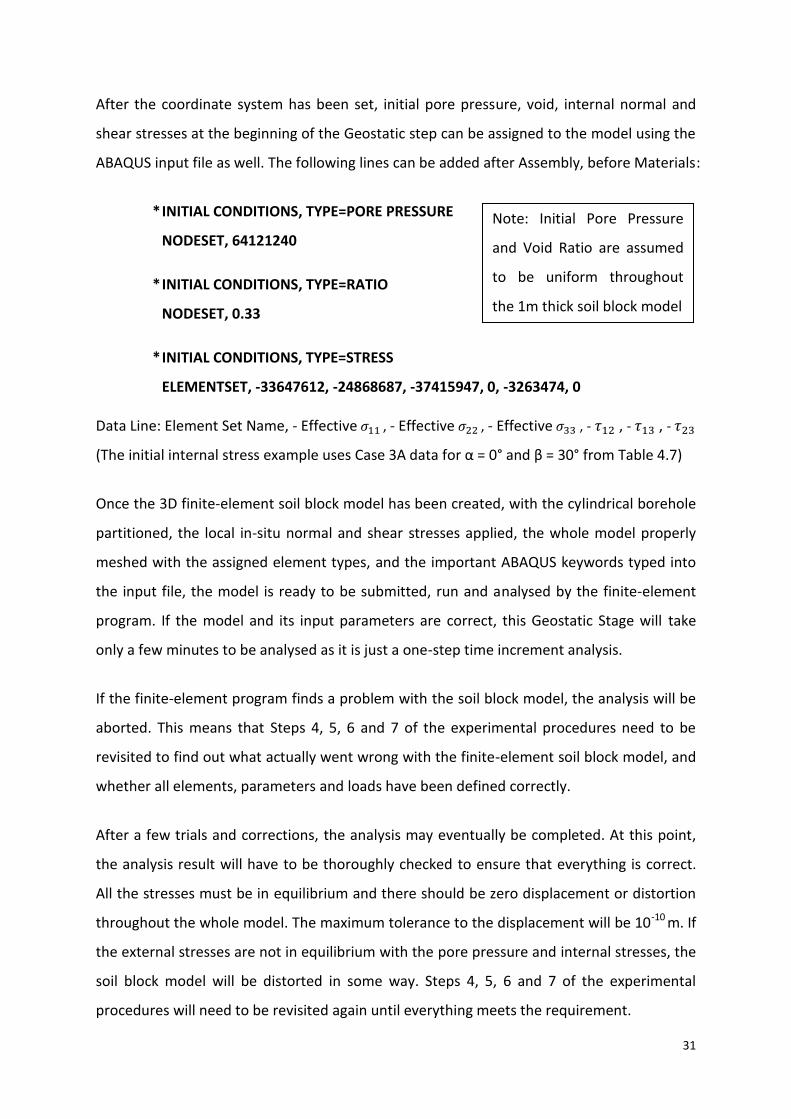
After the coordinate system has been set, initial pore pressure, void, internal normal and
shear stresses at the beginning of the Geostatic step can be assigned to the model using the
ABAQUS input file as well. The following lines can be added after Assembly, before Materials:
* INITIAL CONDITIONS, TYPE=PORE PRESSURE
NODESET, 64121240
* INITIAL CONDITIONS, TYPE=RATIO
NODESET, 0.33
* INITIAL CONDITIONS, TYPE=STRESS
ELEMENTSET, -33647612, -24868687, -37415947, 0, -3263474, 0
Data Line: Element Set Name, - Effective , - Effective , - Effective , - , - , -
(The initial internal stress example uses Case 3A data for α = 0° and β = 30° from Table 4.7)
Once the 3D finite-element soil block model has been created, with the cylindrical borehole
partitioned, the local in-situ normal and shear stresses applied, the whole model properly
meshed with the assigned element types, and the important ABAQUS keywords typed into
the input file, the model is ready to be submitted, run and analysed by the finite-element
program. If the model and its input parameters are correct, this Geostatic Stage will take
only a few minutes to be analysed as it is just a one-step time increment analysis.
If the finite-element program finds a problem with the soil block model, the analysis will be
aborted. This means that Steps 4, 5, 6 and 7 of the experimental procedures need to be
revisited to find out what actually went wrong with the finite-element soil block model, and
whether all elements, parameters and loads have been defined correctly.
After a few trials and corrections, the analysis may eventually be completed. At this point,
the analysis result will have to be thoroughly checked to ensure that everything is correct.
All the stresses must be in equilibrium and there should be zero displacement or distortion
throughout the whole model. The maximum tolerance to the displacement will be 10-10 m. If
the external stresses are not in equilibrium with the pore pressure and internal stresses, the
soil block model will be distorted in some way. Steps 4, 5, 6 and 7 of the experimental
procedures will need to be revisited again until everything meets the requirement.
Note: Initial Pore Pressure
and Void Ratio are assumed
to be uniform throughout
the 1m thick soil block model

32
4.4 The Drilling Stage
In the staged approach analysis, it is extremely important that results from each stage are
being thoroughly checked and verified before feeding them into subsequent stages for
further analysis. This means that if minor problems are not dealt with in the Geostatic Stage,
it can expected that the problems will snowball into larger issues and the final result at the
end of the Drilling Stage will not be accurate at all. Therefore, pore pressure, external and
internal stresses must be in equilibrium at the end of Geostatic Stage and the soil block
model must have zero distortion before the Drilling Stage can commence.
All the displacement boundary conditions and in-situ normal and shear stresses applied on
the wellbore model surfaces are propagated from the Geostatic Stage to the Drilling Stage.
At the end of the Geostatic Stage and before the start of the Drilling Stage, three important
changes will need to take place to change the soil block model into a wellbore model:
(i) Removing the cylindrical borehole section from the soil block model to represent
drilling operations using the Model Change Interaction function available in ABAQUS;
(ii) Replacing the removed cylindrical borehole section with drilling fluid which exerts
hydrostatic pressure onto the borehole surface by applying a mechanical pressure load
onto the borehole surface, where the magnitude will be the same as pore pressure
within the formation to simplify wellbore stability analysis;
(iii) Reapplying the same magnitude of pore pressure to the left, right and back surfaces
only to make them permeable, which also make the top, bottom, front symmetrical and
borehole wall surfaces impermeable, to further simplify the analysis by assuming that
fluid does not flow into the borehole and affect its stability in the drilling stage.
Once these three changes have taken place at the end of the Geostatic Stage and before the
start of the Drilling Stage, the soil block model now becomes a wellbore model. The Drilling
Stage analysis can then be started as the borehole deforms under the existing in-situ normal
and shear stresses propagated from the Geostatic Stage. The Drilling Stage analysis will take
a longer time, ranging from 20 minutes to a few hours, depending on the far-field stress
anisotropy and the elastic or plastic distortion of the borehole elements.

33
Figure 4.5: Drilling Fluid Pressure Supports the Borehole Wall in the Drilling Stage
Figure 4.6: Pore Pressure Applied to Back and Side Surfaces, Others Assumed Impermeable
Similar to the Geostatic Stage, ABAQUS might find problems with the wellbore model and
decides to abort the analysis. Steps 4 to 8 of the experimental procedures may need to be
revisited to debug the problem and rerun the analysis until it can be completed successfully.

34
4.5 Data Extraction and Analysis
The following Field Output Requests will be used across the Geostatic and Drilling Stages:
E - Total Strain Components
EE - Elastic Strain Components
PE - Plastic Strain Components
PEEQ - Equivalent Plastic Strain
POR - Pore Pressure
S - Stress Components and Invariants
U - Translations and Rotations
VOIDR - Void Ratio
The advantages of using ABAQUS is that any of the Field Outputs Requests information can
be extracted from any node point or any element in the finite-element wellbore model at
any time frame across the Geostatic and Drilling Stages. For example, the effective hoop
stress σθ around the wellbore surface halfway between the top and bottom surfaces can be
easily extracted using the Path function in ABAQUS, as shown in Figure 4.6. The middle layer
was chosen because it is the furthest layer away from any edge effects induced by the shear
stresses acting on the top and bottom surfaces. All the information collected from the nodes
along the Path can then be saved, plotted as graphs, compared and analysed. Besides that, a
more general representation of the result can be displayed as coloured contours as well.
Figure 4.7: Circumferential Stress Contours of Case 4B (β = 60°) at the end of Drilling Stage
Path (Node List)
Edge Effects

35
PART 5: RESULTS AND DISCUSSION
The aim of this study is to define a comprehensive method that can transform a vertical
wellbore model into any arbitrarily oriented wellbore model, which can then be reused to
analyse the stability and stress distribution around wellbores at any orientation by changing
the stresses acting on the model. Hence, this study examined the following hypotheses:
Hypothesis 1:
Appropriate sets of normal and shear stresses can be applied to the surfaces of a 3D finite-
element vertical wellbore model to transform it into an inclined wellbore model;
Hypothesis 2:
By applying different sets of normal and shear stresses, the same vertical wellbore model
can be reused and transformed into wellbores at different inclination and orientation;
Hypothesis 3:
The wellbore stability and stress distribution around an arbitrarily oriented and inclined
wellbore can be analysed using a single 3D finite-element vertical wellbore model.
The first part of this study focuses on understanding the mathematical models published by
Jaeger and Cook (1979). Then using the Case 1A isotropic horizontal far-field stresses,
effective hoop stress is plotted against θ and β in Figure 5.1 a-c. This set up a framework in
which the first set of finite-element analysis result may have an established mathematical
model to be compared to and verified with. Once the method of transforming a 3D finite-
element vertical wellbore model into an inclined wellbore is proven to be credible, the
effects of horizontal far-field stress anisotropy on inclined wellbores were further examined.
Table 5.1: Result Figures and Loading Cases
Figures 5.1 a-c 5.2 a-c 5.3 a-c 5.4 a-c 5.5 a-c 5.6 a-c 5.7 a-c 5.8 a-c
Cases 1A 1A 2A 2B 3A 3B 4A 4B
α 0° 0° 0° 90° 0° 90° 0° 90°
Analysis Jaeger &
Cook ABAQUS ABAQUS ABAQUS ABAQUS ABAQUS ABAQUS ABAQUS
σH - σh 0 kPa 4376 kPa 6894 kPa 13790 kPa
Horz Stress
Isotropic Anisotropic Larger Anisotropic Largest
Anisotropic

36
Case 1A: Mathematical model with isotropic loads (σH = σh)
Figures 5.1 a-c plots the effective hoop stress σθ around the wellbore surface ( 0°≤ θ ≤ 180° )
at the end of the drilling stage, at various well inclinations ( 0° ≤ β ≤ 90° ) with azimuth α = 0°.
Equations (1) and (9) were used to generate the plots below.
Figure 5.1a Figure 5.1b
Figure 5.1c
-9.50E+07
-9.00E+07
-8.50E+07
-8.00E+07
-7.50E+07
-7.00E+07
-6.50E+07
-6.00E+07
-5.50E+07
-5.00E+07
-4.50E+07
-4.00E+07
0 30 60 90 120 150 1800
15
30
45
60
75
90
θ
β
σθ (Pa)
0 15 30 45 60 75 90
-9.50E+07
-8.50E+07
-7.50E+07
-6.50E+07
-5.50E+07
-4.50E+07β
σθ (Pa)
0 15 30 45 60 75 90
-9.00E+07
-8.00E+07
-7.00E+07
-6.00E+07
-5.00E+07
-4.00E+07
-3.00E+07
01
83
6
54
72
90
10
8
12
6
14
4
16
2
18
0
θ β
σθ (Pa)

37
Case 1A: ABAQUS finite-element analysis with isotropic loads (σH = σh)
Figures 5.2 a-c plots of effective hoop stress σθ around the wellbore surface ( 0° ≤ θ ≤ 180° )
at the end of drilling stage, at various well inclinations ( 0° ≤ β ≤ 90° ) with azimuth α = 0°.
For isotropic loading, rotating the well in azimuth planes α = 0° and α = 90° give the same
stress distribution. The local in-situ stresses calculated in Table 4.4 were applied to the
finite-element vertical wellbore model to generate these results.
Figure 5.2a Figure 5.2b
Figure 5.2c
-9.50E+07
-9.00E+07
-8.50E+07
-8.00E+07
-7.50E+07
-7.00E+07
-6.50E+07
-6.00E+07
-5.50E+07
-5.00E+07
-4.50E+07
-4.00E+07
0 30 60 90 120 150 180
0
15
30
45
60
75
90
θ
β
σθ (Pa)
0 15 30 45 60 75 90
-9.50E+07
-8.50E+07
-7.50E+07
-6.50E+07
-5.50E+07
-4.50E+07β
σθ (Pa)
0 15 30 45 60 75 90
-9.50E+07
-8.50E+07
-7.50E+07
-6.50E+07
-5.50E+07
-4.50E+07
-3.50E+0701
83
6
54
72
90
10
8
12
6
14
4
16
2
18
0
θ β
σθ (Pa)

38
5.1 Comparing Mathematical and ABAQUS Models under Isotropic Loads
Figures 5.1 a-c and Figures 5.2 a-c are almost identical with each other despite the fact that
one is produced using theoretical mathematical equations, and the other using a vertical
finite-element wellbore model that is transformed into various inclined wellbores models.
This was achieved by applying a set of pre-calculated normal and shear stresses onto the
vertical wellbore surfaces, which effectively created the conditions as if the analyses were
done using full inclined wellbore model, as shown in Figure 3.9.
If several inclined wellbore models with different borehole inclinations were used to analyse
the same problem, then the conventional method is expected to generate effective hoop
stress plots similar to Figures 5.1 a-c. However, this may take a lot of time as it is not easy
than to build a finite-element model, let alone a few of them with different specifications.
Hence, if there is a simpler and more effective way of creating an inclined borehole, then
the method should seriously be considered as it can save a lot of time and resources.
Both Figures 5.1b and 5.2b shows that stress anisotropy around the borehole surface is
minimum a when β=0°. This means that both the mathematical theory and finite element
result agrees that a vertical wellbore is most stable under isotropic horizontal stress. Besides
that, both analysis also agree with each other that maximum stress anisotropy occurs when
β=90°, i.e. when the wellbore is horizontal. The magnitudes of stress are almost identical
and the nodes on Figures 5.1a and 5.2a occur around the same value of θ as well.
With so many similarities, it can be said that a 3D finite-element vertical wellbore model can
be transformed into an inclined wellbore model by applying appropriate sets of normal and
shear stresses to the vertical wellbore model surfaces, under the condition that the normal
and shear stresses are calculated using the mathematical equations put forward in Part 3
and 4 if this report. Hence, Hypothesis 1 has been proven to be correct.
At the same time, as different sets of normal and shear stresses calculated in Table 4.4 has
been applied to the same vertical wellbore model and it has been reused many times to
analyse the stress distribution around the boreholes at different inclination and orientation.
Hence, Hypothesis 2 can be proven correct as well.

39
Case 2A: ABAQUS analysis with anisotropic loads (σH - σh = 4676 kPa) and α = 0°
Plots of effective hoop stress σθ around the wellbore surface ( 0° ≤ θ ≤ 180° ) at the end of
drilling step, at various well inclinations ( 0° ≤ β ≤ 90° ) rotating in the α = 0° azimuth plane,
perpendicular to the minimum horizontal stress axis.
Figure 5.3a Figure 5.3b
Figure 5.3c
-1.00E+08
-9.00E+07
-8.00E+07
-7.00E+07
-6.00E+07
-5.00E+07
-4.00E+07
-3.00E+07
0 30 60 90 120 150 1800
15
30
45
60
75
90
θ
β
σθ (Pa)
0 15 30 45 60 75 90
-1.00E+08
-9.00E+07
-8.00E+07
-7.00E+07
-6.00E+07
-5.00E+07
-4.00E+07
-3.00E+07β
σθ (Pa)
0 15 30 45 60 75 90
-1.00E+08
-9.00E+07
-8.00E+07
-7.00E+07
-6.00E+07
-5.00E+07
-4.00E+07
-3.00E+07
-2.00E+07
01836547290
10
8
12
6
14
4
16
2
18
0
θ β σθ (Pa)
40
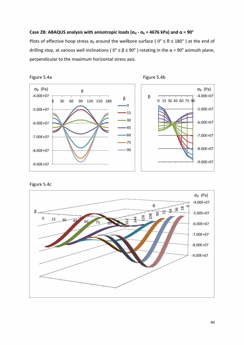
Case 2B: ABAQUS analysis with anisotropic loads (σH - σh = 4676 kPa) and α = 90°
Plots of effective hoop stress σθ around the wellbore surface ( 0° ≤ θ ≤ 180° ) at the end of
drilling step, at various well inclinations ( 0° ≤ β ≤ 90° ) rotating in the α = 90° azimuth plane,
perpendicular to the maximum horizontal stress axis.
Figure 5.4a Figure 5.4b
Figure 5.4c
-9.00E+07
-8.00E+07
-7.00E+07
-6.00E+07
-5.00E+07
-4.00E+07
0 30 60 90 120 150 1800
15
30
45
60
75
90
θ
β
σθ (Pa)
0 15 30 45 60 75 90
-9.00E+07
-8.00E+07
-7.00E+07
-6.00E+07
-5.00E+07
-4.00E+07β
σθ (Pa)
0 15 30 45 60 75 90
-9.00E+07
-8.00E+07
-7.00E+07
-6.00E+07
-5.00E+07
-4.00E+07
0
18
36
54
72
90
10
8
12
6
14
4
16
2
18
0
θ β
σθ (Pa)

41
Case 3A: ABAQUS analysis with larger anisotropic loads (σH - σh = 6895 kPa) and α = 0°
Plots of effective hoop stress σθ around the wellbore surface ( 0° ≤ θ ≤ 180° ) at the end of
drilling step, at various well inclinations ( 0° ≤ β ≤ 90° ) rotating in the α = 0° azimuth plane,
perpendicular to the minimum horizontal stress axis.
Figure 5.5a Figure 5.5b
Figure 5.5c
-1.00E+08
-9.00E+07
-8.00E+07
-7.00E+07
-6.00E+07
-5.00E+07
-4.00E+07
-3.00E+07
0 30 60 90 120 150 1800
15
30
45
60
75
90
θ
β
σθ (Pa)
0 15 30 45 60 75 90
-1.00E+08
-9.00E+07
-8.00E+07
-7.00E+07
-6.00E+07
-5.00E+07
-4.00E+07
-3.00E+07
-2.00E+07β
σθ (Pa)
0 15 30 45 60 75 90
-1.00E+08
-9.00E+07
-8.00E+07
-7.00E+07
-6.00E+07
-5.00E+07
-4.00E+07
-3.00E+07
-2.00E+07
01836547290
10
8
12
6
14
4
16
2
18
0 θ β σθ (Pa)

42
Case 3B: ABAQUS analysis with larger anisotropic loads (σH - σh = 6895 kPa) and α = 90°
Plots of effective hoop stress σθ around the wellbore surface ( 0° ≤ θ ≤ 180° ) at the end of
drilling step, at various well inclinations ( 0° ≤ β ≤ 90° ) rotating in the α = 90° azimuth plane,
perpendicular to the maximum horizontal stress axis.
Figure 5.6a Figure 5.6b
Figure 5.6c
-9.00E+07
-8.00E+07
-7.00E+07
-6.00E+07
-5.00E+07
-4.00E+07
0 30 60 90 120 150 1800
15
30
45
60
75
90
θ
β
σθ (Pa)
0 15 30 45 60 75 90
-9.00E+07
-8.00E+07
-7.00E+07
-6.00E+07
-5.00E+07
-4.00E+07β
σθ (Pa)
0 15 30 45 60 75 90
-9.00E+07
-8.00E+07
-7.00E+07
-6.00E+07
-5.00E+07
-4.00E+07
0
18
36
54
72
90
10
8
12
6
14
4
16
2
18
0
θ β
σθ (Pa)

43
Case 4A: ABAQUS analysis with largest anisotropic loads (σH - σh = 13790 kPa) and α = 0°
Plots of effective hoop stress σθ around the wellbore surface ( 0° ≤ θ ≤ 180° ) at the end of
drilling step, at various well inclinations ( 0° ≤ β ≤ 90° ) rotating in the α = 0° azimuth plane,
perpendicular to the minimum horizontal stress axis.
Figure 5.7a Figure 5.7b
Figure 5.7c
-1.00E+08
-9.00E+07
-8.00E+07
-7.00E+07
-6.00E+07
-5.00E+07
-4.00E+07
-3.00E+07
-2.00E+07
0 30 60 90 120 150 1800
15
30
45
60
75
90
0 15 30 45 60 75 90
-1.00E+08
-9.00E+07
-8.00E+07
-7.00E+07
-6.00E+07
-5.00E+07
-4.00E+07
-3.00E+07
-2.00E+07
0 15 30 45 60 75 90
-1.00E+08
-9.00E+07
-8.00E+07
-7.00E+07
-6.00E+07
-5.00E+07
-4.00E+07
-3.00E+07
-2.00E+07
01836547290
10
8
12
6
14
4
16
2
18
0
θ
β
σθ (Pa)
β
σθ (Pa)
θ β
σθ (Pa)

44
Case 4B: ABAQUS analysis with largest anisotropic loads (σH - σh = 13790 kPa) and α = 90°
Plots of effective hoop stress σθ around the wellbore surface ( 0° ≤ θ ≤ 180° ) at the end of
drilling step, at various well inclinations ( 0° ≤ β ≤ 90° ) rotating in the α = 90° azimuth plane,
perpendicular to the maximum horizontal stress axis.
Figure 5.8a Figure 5.8b
Figure 5.8c
0 15 30 45 60 75 90
-9.00E+07
-8.00E+07
-7.00E+07
-6.00E+07
-5.00E+07
-4.00E+07
-3.00E+07
-2.00E+07
-9.00E+07
-8.00E+07
-7.00E+07
-6.00E+07
-5.00E+07
-4.00E+07
-3.00E+07
-2.00E+07
0 30 60 90 120 150 180
0
15
30
45
60
75
90
0 15 30 45 60 75 90
-9.00E+07
-8.00E+07
-7.00E+07
-6.00E+07
-5.00E+07
-4.00E+07
-3.00E+07
-2.00E+07
0
18
36
54
72
90
10
8
12
6
14
4
16
2
18
0
θ
β
σθ (Pa)
β
σθ (Pa)
θ
β
σθ (Pa)

45
5.2 Comparison of results with data published by Zhou et al (1996)
Case 2B: Anisotropy Case 3B: Larger Anisotropy Case 4B: Largest Anisotropy = 0.2, = 0.78, = 0.66 = 0.2, = 0.81, = 0.63 = 0.2, = 0.90, = 0.55
Figure 5.9: The drilling direction (α) in the chart below by Zhou et al (1996) is equal to 90°,
which is comparable to Cases 2B, 3B and 4B in this study. It plots the deviation angle from
vertical (β) at which stress anisotropy around the well wall is minimised in extensional stress
regimes with = 0 and = 0.25, slightly higher than the = 0.2 used in Cases 2B, 3B and 4B.
0 15 30 45 60 75 90
-9.00E+07
-8.00E+07
-7.00E+07
-6.00E+07
-5.00E+07
-4.00E+07
-3.00E+07
-2.00E+07σθ (Pa) β
0 15 30 45 60 75 90
-9.00E+07
-8.00E+07
-7.00E+07
-6.00E+07
-5.00E+07
-4.00E+07σθ (Pa) β
0 15 30 45 60 75 90
-9.00E+07
-8.00E+07
-7.00E+07
-6.00E+07
-5.00E+07
-4.00E+07β σθ (Pa)
𝑛𝐻
𝜎𝐻 / 𝜎𝑣
𝑛 𝜎 / 𝜎𝑣
𝟐𝑩*
𝟑𝑩*
𝟒𝑩*
𝟏𝑨
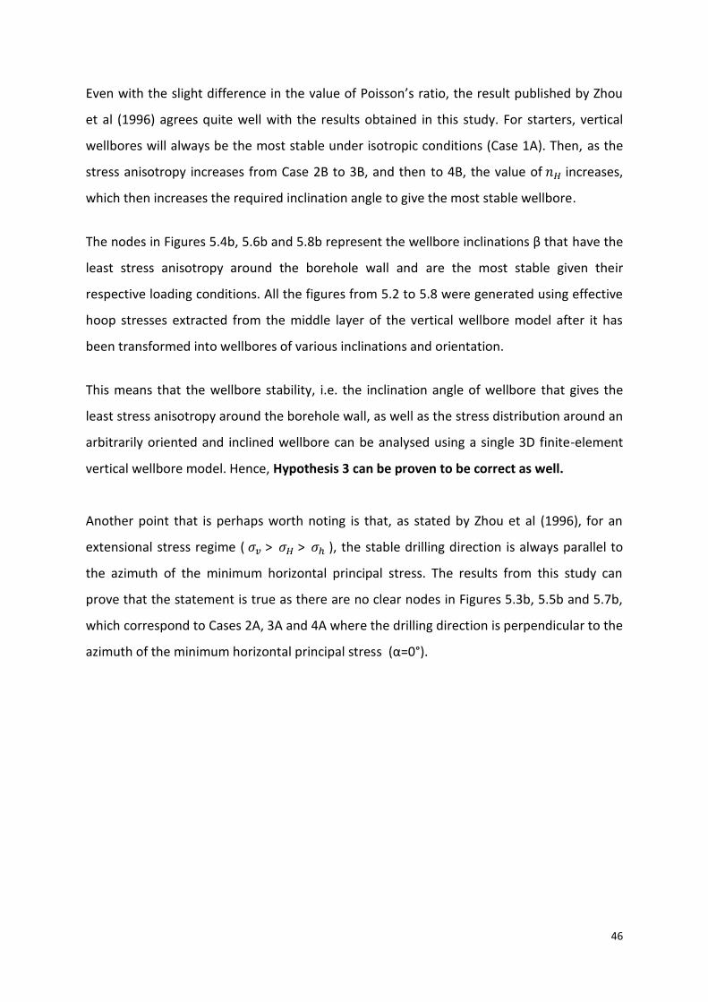
46
Even with the slight difference in the value of Poisson’s ratio, the result published by Zhou
et al (1996) agrees quite well with the results obtained in this study. For starters, vertical
wellbores will always be the most stable under isotropic conditions (Case 1A). Then, as the
stress anisotropy increases from Case 2B to 3B, and then to 4B, the value of increases,
which then increases the required inclination angle to give the most stable wellbore.
The nodes in Figures 5.4b, 5.6b and 5.8b represent the wellbore inclinations β that have the
least stress anisotropy around the borehole wall and are the most stable given their
respective loading conditions. All the figures from 5.2 to 5.8 were generated using effective
hoop stresses extracted from the middle layer of the vertical wellbore model after it has
been transformed into wellbores of various inclinations and orientation.
This means that the wellbore stability, i.e. the inclination angle of wellbore that gives the
least stress anisotropy around the borehole wall, as well as the stress distribution around an
arbitrarily oriented and inclined wellbore can be analysed using a single 3D finite-element
vertical wellbore model. Hence, Hypothesis 3 can be proven to be correct as well.
Another point that is perhaps worth noting is that, as stated by Zhou et al (1996), for an
extensional stress regime ( > > ), the stable drilling direction is always parallel to
the azimuth of the minimum horizontal principal stress. The results from this study can
prove that the statement is true as there are no clear nodes in Figures 5.3b, 5.5b and 5.7b,
which correspond to Cases 2A, 3A and 4A where the drilling direction is perpendicular to the
azimuth of the minimum horizontal principal stress (α=0°).

47
PART 6: CONCLUSIONS
3D finite-element vertical wellbore models can be transformed into any arbitrarily oriented
wellbore models by applying a set of appropriate normal and shear stresses on the model
surfaces. Depending on the desired wellbore inclination and orientation, the magnitude and
direction of these in-situ stresses can then be calculated from the far-field principal stresses
using mathematical equations published by Jaeger and Cook (1979).
Once a set of normal and shear stresses for a particular inclination and orientation has been
determined, researchers can apply them to the vertical finite-element wellbore model to
transform it into an inclined wellbore model. The wellbore stability and stress distribution
around the wellbore at that particular inclination and orientation can then be analysed.
This wellbore transformation method allows the same vertical model to be used repeatedly
to analyse the wellbore characteristics at any other desired inclination and orientation.
Unlike conventional methods where inclined wellbore models have pre-drilled boreholes set
at one inclination only, and a lot of models may be required to analyse a range of wellbore
inclinations, this wellbore transformation method only needs a single 3D vertical wellbore
model and it can analyse limitless amount of wellbore inclination and orientation.
PART 7: FUTURE WORKS
The wellbore transformation method has been conducted using a symmetrical half-vertical
wellbore model for inclinations 0° ≤ β ≤ 90° but only in azimuth planes α = 0° and α = 90°. A
full-vertical wellbore model should to be tested for wellbore transformation in any azimuth
plane and any inclination. The full stress transformation matrix, i.e. Equation (1), may need
to be used and the plane stress transformation equations cannot be used anymore.
On the other hand, the Staged Approach can be extended to include Cement and Casing,
Hydraulic Fracturing, Completion as well as Production Stages to the vertical wellbore model
and a range of other research topics like cement sheath integrity, hydraulic fracturing or
sand production in an arbitrarily oriented borehole can be examined.

48
PART 8: REFERENCES
1 SPEUK (2005): SPEreview, Issue 187, Jun 2005,
http://speuk.spe.org/images/speuk/articles/52/JUNE_2005.pdf 2 Kang, Y., Yu, M., Miska, S., Takach, N.E. (2009) “Wellbore Stability: A Critical Review and
Introduction to DEM”, SPW 124669, SPE Annual Technical Conference, New Orleans, Louisiana, 4 – 7 Oct 2009
3 Collins, P.M. (2002) “Geomechanics and wellbore stability design of an offshore horizontal
well, North Sea”, SPE 78975, SPE International Thermal Operations and Heavy Oil Symposium and International Horizontal Well Technology Conference, Calgary, Alberta, Canada, 4 – 7 Nov 2002
4 Land, W.J., Jett, M.B. (1990) “High Expectations for Horizontal Drilling Becoming Reality”,
Oil Field Journal, 24 Sep 1990, 7, pp 70-79 5 Schlumberger Ltd. (2011) “Development of Directional-Drilling Technology”, Oilfield
Review Interactive, Number 2, http://www.slb.com/resources/publications/oilfield_review/ori/ori002/01/01a.aspx
6 Zhou, S., Hills, R.R., Sandiford, M. (1996) “On the Mechanical Stability of Inclined
Wellbores”, SPE 28176, SPE Drilling & Completion, Volume 11, Number 2, Jun 1996, pp 67-72
7 Awal, M.R., Khan, M.S., Mohiuddin, M.A., Abdulrahem, A., Azeemuddin, M.A. (2001) “ A
New Approach to Borehole Trajectory Optimisation for Increased Hole Stability”, SPE 68092, SPE Middle East Oil Show, Bahrain, 17-20 Mar 2001
8 Maury, V. (1994) “Rock Failure Mechanisms Identification: A key for Wellbore Stability and
Reservoir Behaviour Problem”, SPE 28049, Rock Mechanics in Petroleum Engineering, Delft, Netherlands
9 Bradley, W.B. (1979a) “Mathematical Concept – Stress Cloud Can Predict Borehole
Failure”, The Oil and Gas Journal, Feb 1979 10 Bradley, W.B. (1979b) “Failure of Inclined Boreholes”, Journal of Energy Resources
Technology, Transactions of ASME, Dec 1979, 101, pp 232-239 11 Hsiao, C. (1988) “A Study of Horizontal-Wellbore Failure”, SPE Production Engineering,
Volume 3, Number 4, Nov 1988, pp 489-494 12 Yew, C.H., Li, Y. (1988) “Fracturing of a Deviated Well”, SPE Production Engineering,
Volume 3, Number 4, Nov 1988, pp 429-437

49
13 Gray, K.E., Podnos, E., Becker, E. (2007) “Finite-Element Studies of Near-Wellbore Region
During Cementing Operations: Part I”, SPE 106998, Production and Operations Symposium, Oklahoma, 31 Mar-3 Apr 2007
14 SIMULIA, ABAQUS 6.10 Documentation, Reference and User’s Manuals,
http://www.simulia.com/support/documentation.html 15 Pattillo, P.D., Krestiansen, T.G. (2002) “Analysis of Horizontal Casing Integrity in the
Valhall Vield”, SPE 78204, SPE/ISRM Rock Mechanic Conference, Irving, Texas, 20-23 Oct 2002
16 Jo, H., Gray, K.E. (2010) “Mechanical Behaviour of Concentric Casing, Cement, And
Formation Using Analytical and Numerical Methods”, ARMA 10-142, 44th US Rock Mechanic Symposium and 5th US-Canada Rock Mechanics Symposium, Salt Lake City, UT, 27-30 Jun 2010
17 Nouri, A., Vaziri, H., Kuru, E. (2006) “Numerical Investigation on Sand Production Under
Realistic Reservoir / Well Flow Conditions”, Canadian International Petroleum Conference, Calgary, Alberta, 13-15 Jun 2006
18 Bahrami, V., Mortazavi, A. (2008) “A Numerical investigation of Hydraulic Fracturing
Process in Oil Reservoirs Using Non-Linear Fracture Mechanics”, ARMS5-2008-120, ISRM International Symposium 5th Asian Rock Mechanics Symposium, Tehran, Iran, 24-26 Nov 2008
19 Jaeger, J.C., Cook, N.G.W. (1979), Fundamentals of Rock Mechanics, 3rd edition, Chapman
and Hall, London 20 Fjaer, E., Holt, R.M., Horsrud, P., Raaen, A.M., Risnes, R. (2008) “Chapter 4: Stresses
around boreholes. Borehole failure criteria”, Petroleum Related Rock Mechanics, 2nd edition, Elsevier, Amsterdam, pp 135-150
21 Crandall, S.H., Dahl, N.C., Lardner, T.J. (1972) “Stress and Strain”, An Introduction to the
Mechanics of Solids, 2nd edition, McGraw-Hill, New York, pp 214-221