Finite element method for stability and vibration analyses of thin-

walled beams with arbitrary cross-section

*M. Soltani1), B. Asgarian2), and F. Mohri3)

1) ,2) Civil Engineering Faculty, K.N.Toosi university of Technology, Tehran, Iran 1) msoltani2@yahoo.com

3) Université de Lorraine, Laboratoire d'Etude des Microstructures et de Mécanique des

Matériaux (LEM3), Metz. France

ABSTRACT In this paper, a generalized numerical and theoretical method is presented for the free vibration and stability analyses of tapered thin-walled beams with non-symmetric cross-section. The total potential energy is derived for an elastic behavior from the strain energy, the kinetic energy and work of the applied loads. Free vibration is considered in presence of harmonic excitations. The effects of the initial stresses and load eccentricities are also considered in the study. The governing equilibrium equations, motion equations and the associated boundary conditions are determined from the stationary condition. …… 1. INTRODUCTION The use of thin-walled beams with I, Z and C cross sections has been increasing in many steel constructions due to their ability to utilize structural material more efficiently and optimize the distribution of weight. Flexural-torsional stability and vibration analyses are important topics in the design of these structures and research of accurate models has interested many researchers over the world from the last mid century until now. Since the early works of (Timoshenko 1961) and (Vlasov 1959) there have been extensive investigations on the elastic flexural-torsional buckling behavior of thin walled beam members. In these investigations, (Chen 1987) and (Bazant 1991), the buckling loads were evaluated either by closed-form solutions of the fourth-order differential equations governing the twisting and bending of the thin-walled beams or by using of complementary energy principle. Mentioned studies were focused on the stability and vibration analyses of prismatic thin-walled beams. However, in the last decades, thin-walled beams with variable cross-sections are extensively adopted in 1 PhD Candidate 2 Associate Professor 3 Assistant Professor

1403

different steel constructions. The investigations of elastic flexural-torsional buckling and vibration modes of tapered thin-walled with the use of efficient numerical techniques such as finite element method in the validation process has attracted many researchers. Among the first investigations on this topic, the most important ones are the studies of (Yang 1987) who formulated a finite element model for the beam that takes into account the effect of non-uniform torsion. More recently, (Kim 2000) investigated the linear stability and free vibration behavior of doubly symmetric I tapered thin-walled beams by a finite element approach. A theoretical model for large torsion context and equivalent beam finite element formulation in finite torsion amplitudes were developed by (Ronagh 2000). (Chen 2000) applied Hamilton’s principle to the potential energy and obtained the motion equations governing of non-prismatic thin-walled beams. Based on the Rayleigh-Ritz method, a general variational formulation to analyze the lateral-torsional buckling behavior of tapered thin-walled beams with singly symmetric cross-sections was presented by (Andrade 2007). In (Asgarian 2013), the lateral torsional behavior of tapered beams with singly symmetric I cross-sections was studied. The previous work is extended to include eccentrically axial forces and dynamic loads for beams with non-symmetric cross-sections. 2. DERIVATION OF EQUILIBRIUM AND MOTION EQUATIONS FOR BUCKLING AND FREE VIBRATION 2.1. Kinematics A tapered thin-walled beam with arbitrary cross-section is considered in the study (Fig.1a). A direct rectangular co-ordinate system is chosen, with x the initial longitudinal axis and y and z the first and second main bending axes. The origin of these axes is located at the centroid O. The shear centre with co-ordinates (yc, zc) in xyz is denoted C (Fig.1b). In the present study, the beam is subjected to arbitrary distributed force px in structural domain in x direction. Under these conditions, the three displacement components of a point M on the section contour can be expressed as function of those of the shear center C:

xxzy

xxxyxwz

xxxzxvyxuzyxU cc

)(),())()()(())()()(()(),,( 0

(1)

)())(()(),,( xxzzxvzyxV c (2)

)())(()(),,( xxyyxwzyxW c (3)

In which U represents the axial displacement. The displacement components V and W represent lateral and vertical displacements (in y and z directions). The torsion angle is denoted by . The term ),( zy is the warping function, which can be defined based on Saint Venant’s torsion theory. The Green’s strain tensor components which incorporate the large displacements and including linear and non-linear strain part are given by:

1404

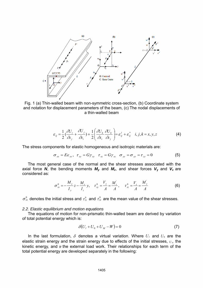
Fig. 1 (a) Thin-walled beam with non-symmetric cross-section, (b) Coordinate system

and notation for displacement parameters of the beam, (c) The nodal displacements of a thin-walled beam

zyxkjixU

xU

xU

xU

ijlij

j

k

i

k

i

j

j

iij ,,,,

21)(

21 *

(4)

The stress components for elastic homogeneous and isotropic materials are:

0 , zyyyyyxzxzxyxyxxxx GGE (5)

The most general case of the normal and the shear stresses associated with the axial force N, the bending moments My and Mz, and shear forces Vy and Vz are considered as:

, ,

'0

'00

AM

AV

AM

AV

yI

Mz

IM yz

xzzy

xyz

z

y

yxx

(6)

0xx denotes the initial stress and 0

xy and 0xz are the mean value of the shear stresses.

2.2. Elastic equilibrium and motion equations The equations of motion for non-prismatic thin-walled beam are derived by variation of total potential energy which is:

00 WUUU Ml (7)

In the last formulation, denotes a virtual variation. Where lU and 0U are the elastic strain energy and the strain energy due to effects of the initial stresses, MU the kinetic energy, and W the external load work. Their relationships for each term of the total potential energy are developed separately in the following:

1405

dxupW

dAdxVVWWUUU

dAdxU

dAdxGGEU

LPx

L

AM

L

A xzxzxyxyxxxx

L

A

lxy

lxz

lxy

lxy

lxx

lxxl

0

2

0

*0*0*00

0)()()(

(8)

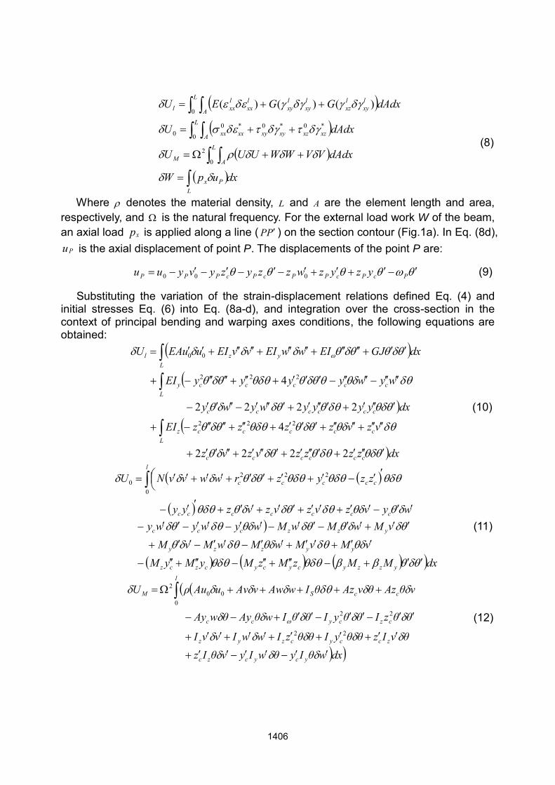
Where denotes the material density, L and A are the element length and area, respectively, and is the natural frequency. For the external load work W of the beam, an axial load xp is applied along a line ( PP ) on the section contour (Fig.1a). In Eq. (8d),

Pu is the axial displacement of point P. The displacements of the point P are:

PcPcPPcPcPPP yzyzwzzyzyvyuu 000 (9)

Substituting the variation of the strain-displacement relations defined Eq. (4) and initial stresses Eq. (6) into Eq. (8a-d), and integration over the cross-section in the context of principal bending and warping axes conditions, the following equations are obtained:

dxzzzzvzvz

vzvzzzzEI

dxyyyywywy

wywyyyyEI

dxGJEIwwEIvvEIuuEAU

cccccc

Lcccccz

cccccc

Lcccccy

Lyzl

2222

4

2222

4

222

222

00

(10)

dxMMzMzMyMyMvMvMwMwMvM

vMwMwMwywywywyvzvzvzvzyy

zzyzrwwvvNU

yzzycycyczcz

yyzzy

yzzccc

ccccccc

l

ccccc

0

2220

(11)

dxwθIyθwIyvθIzθvIzθθyIθθzIwwIvvI

θθzIθθyIθθIwθAyθwAy

vθAzθvAzθIwAwvAvuAuρU

ycyczc

zccyczyz

czcycc

l

ccSM

22

220

002

(12)

1406

dxByMyMwM

zMzMvMupW

cycyy

l

czczzx

0000

0 0000

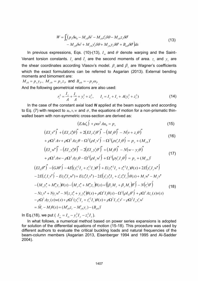
(13)

In previous expressions, Eqs. (10)-(13), I and denote warping and the Saint-Venant torsion constants. yI and zI are the second moments of area. cz and cy are

the shear coordinates according Vlasov’s model. y and z are Wagner’s coefficients which the exact formulations can be referred to Asgarian (2013). External bending moments and bimoment are:

Pxz ypM 0 , Pxy zpM 0 and PxpB 0 . And the following geometrical relations are also used:

)( , 22222

cczyscczy

c zyAIIIzyAI

AI

r

(14)

In the case of the constant axial load N applied at the beam supports and according to Eq. (7) with respect to wvu , ,0 and , the equations of motion for a non-prismatic thin-walled beam with non-symmetric cross-section are derived as:

xpAuuEA

02

0 (15)

)(

2

02222

zyzczc

cyczczz

MpIzvIAzAv

zvNMzEIzEIvEI

(16)

)(

2

02222

yzycyc

czcycyy

MpIywIAyAw

ywNMyEIyEIwEI

(17)

)()( )(ˆ)()()()(

)()()()(

)()(

)(2)()(2

2)()()(4

000

222222

222

2

2222

ByMzMxMM

wyIvzIxIzIyxwxAyxvxAzIxIxyyzzNwNyvNz

rNMMxzMzMxyMyM

vMwMxIzzIyyEvIzEwIyEvIzE

wIyExIzIyEIzIyEGJEI

cycztt

cyczzcycc

cωscccccc

czyyzcycyczcz

yzzccycczcyczc

yczcyczcycω

(18)

In Eq.(18), we put ( zcycωω IzIyII 22 ). In what follows, a numerical method based on power series expansions is adopted for solution of the differential equations of motion (15-18). This procedure was used by different authors to evaluate the critical buckling loads and natural frequencies of the beam-column members (Asgarian 2013, Eisenberger 1994 and 1995 and Al-Sadder 2004).

1407

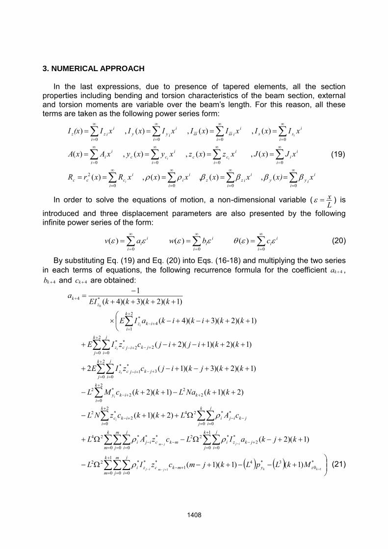
3. NUMERICAL APPROACH In the last expressions, due to presence of tapered elements, all the section properties including bending and torsion characteristics of the beam section, external and torsion moments are variable over the beam’s length. For this reason, all these terms are taken as the following power series form:

0000

2

0000

0000

(,)(,)(,)(

)(, )(, )(, )(

)(, )(, )(, )

i

iiyy

i

iizz

i

ii

i

iccc

i

ii

i

icc

i

icc

i

ii

i

iss

i

ii

i

iiyy

i

iizz

xx) xx xx xRxrR

xJxJ xzxzxyxy xAxA

xIxI xIxI xIxI xI(xI

i

ii

i

(19)

In order to solve the equations of motion, a non-dimensional variable ( Lx ) is

introduced and three displacement parameters are also presented by the following infinite power series of the form:

000

)( )( )(i

ii

i

ii

i

ii cbwav (20)

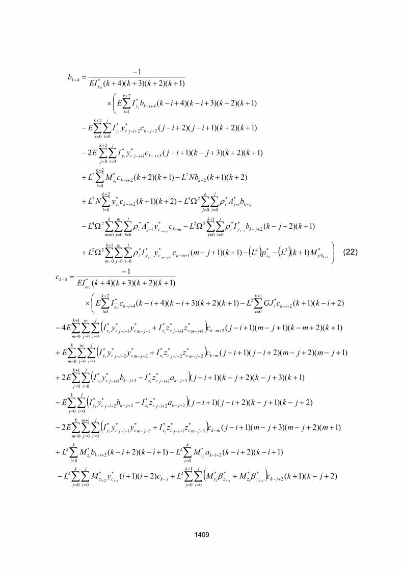
By substituting Eq. (19) and Eq. (20) into Eqs. (16-18) and multiplying the two series in each terms of equations, the following recurrence formula for the coefficient 4ka ,

4kb and 4kc are obtained:

)1()1)(1(

)1)(2(

)2)(1(

)2)(1()1)(2(

)1)(2)(3)(1(2

)1)(2)(1)(2(

)1)(2)(3)(4(

)1)(2)(3)(4(1

*0

3*41

0 0 01

***22

1

0 02

**22

0 0 0

***24

0 0

**242

02

*2

22

2

02

2

2

0 031

**

2

0 022

**

2

14

*

*4

11

0

kkjmij

ijjm

i

i

i

i

i

zy

k

m

m

j

j

imkczi

k

j

j

ijkzi

k

m

m

j

j

imkciji

k

j

j

ijkiji

k

iikc

k

k

iik

*y

k

j

j

ijkijcz

k

j

j

ijkijcz

k

iikz

zk

MkLpLkjmczIL

kjkaILczAL

cALkkczNL

kkNaLkkcML

kkjkijczIE

kkijijczIE

kkikikaIE

kkkkEIa

(21)

1408

)1()1)(1(

)1)(2(

)2)(1(

)2)(1( )1)(2(

)1)(2)(3)(1( 2

)1)(2)(1)(2(

)1)(2)(3)(4(

)1)(2)(3)(4(1

*0

3*41

0 0 01

***22

1

0 02

**22

0 0 0

***24

0 0

**242

02

*2

22

2

02

2

2

0 031

**

2

0 022

**

2

14

*

*4

11

0

kkjmij

ijjm

i

i

i

i

i

yz

k

m

m

j

j

imkcyi

k

j

j

ijkyi

k

m

m

j

j

imkciji

k

j

j

ijkiji

k

iikc

k

k

iik

*z

k

j

j

ijkijcy

k

j

j

ijkijcy

k

iiky

yk

MkLpLkjmcyIL

kjkbILcyAL

bALkkcyNL

kkNbLkkcML

kkjkijcyIE

kkijijcyIE

kkikikbIE

kkkkEIb

(22)

1

0 02

****2

0 0

*2

02

2

02

2

0

1

0 03

*1

**3

*1

**

0 022

**22

**

1

0 031

**31

**

0 0 02

*2

**2

*2

**

1

0 0 021

*1

**1

*1

**

1

02

*22

14

*

*4

)2)(1()2)(1(

)1)(2( )1)(2(

)1)(2)(3)(1(2

)2)(1)(2)(1(

)1)(3)(2)(1(2

)1)(2)(2)(1(

)1)(2)(1)(1(4

)2)(1()1)(2)(3)(4(

)1)(2)(3)(4(1

2

0

k

j

j

ijkyzzy

k

j

j

ijkc

*z

k

iik

*y

k

iik

*z

k

m

m

j

j

imkjmcijczjmcijcy

k

j

j

ijkijczjkijcy

k

j

j

ijkijczjkijcy

k

m

m

j

j

imkjmcijczjmcijcy

k

m

m

j

j

imkjmcijczjmcijcy

k

iiki

k

iik

k

jkkcMMLciiyML

ikikaMLikikbML

mjmjmijczzIyyIE

jkjkijijazIbyIE

kjkjkijazIbyIE

jmjmijijczzIyyIE

kmkjmijczzIyyIE

ikkcGJLkkikikcIE

kkkkEIc

ijiijiiji

ii

ii

ii

ii

ii

ii

i

1409

)1()1()1(

)1)(1(

)1)(1(

)1)(1(

)2)(1(

)2)(1(

)2)(1()2)(1(

)1)(2()2)(1(

)2)(1()2)(1(

*0

3

0

*0

*

0

*0

*3

0 0 01

***22

0 0 01

***22

0 0 0

***24

0 0 0 0

*******22

0 0 0

***241

0 02

**22

0 0

**24

0 0

****2

02

*2

02

*2

1

02

*2

0 0

*2

0 0

*2

0 0

*2

111

1

1

1111

22

2

22

kBLikMyikMzL

mkjmbyIL

mkjmazILbyAL

mnjmczzIyyIL

azALjkkcIL

cILijijcyyzzNL

ikikbyNLikikazNL

kikcRNLciizML

cijijyMLcijijzML

kikiiki

jmij

jmijjm

mnjmijmnjmij

jmij

ijijiiji

ii

iiji

ijiiji

k

iyc

k

izc

k

m

m

j

j

imkcyi

k

m

m

j

j

imkczi

k

m

m

j

j

imkciji

nk

k

n

n

m

m

j

j

icczccyi

k

m

m

j

j

imkciji

k

j

j

ijki

k

j

j

ijksi

k

j

j

ijkcccc

k

iikc

k

iikc

k

iikc

k

j

j

ijkc

*y

k

j

j

ijkc

*z

k

j

j

ijkc

*y

(23)

Where

i

iyyi

izzi

iyyi

izz

iiωiω

iiyy

iizz

iii

icc

icc

iii

icc

iii

iisis

iii

iiyy

iizz

LMMLMMLMMLMM

LBBLLL

LyyLzzLAALRR

LJJLIILIILIILII

iiii

ii

iiiiii

ii

0*

00*0

**

0*

0***

****

*****

, , , ,

, , , ,

, , , ,

, , , ,

(24)

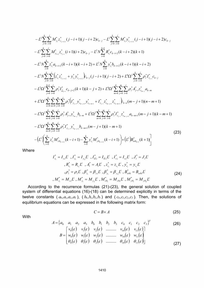
According to the recurrence formulas (21)-(23), the general solution of coupled system of differential equations (16)-(18) can be determined explicitly in terms of the twelve constants ( 3210 ,,, aaaa ), ( 3210 ,,, bbbb ) and ( 3210 ,,, cccc ). Then, the solutions of equilibrium equations can be expressed in the following matrix form: ABC (25) With

TccccbbbbaaaaA 321032103210 (26)

1110210

1110210

1110210

..........

..........

.......... wwwww

vvvvvB

(27)

1410

wv

C

(28)

All terms of iv , iw and i are derived with the aid of the symbolic software MATLAB. 4. BOUDARY CONDITIONS AND SHAPE FUNCTION

Knowing that the all undefined coefficients ( 3210 ,,, aaaa ), ( 3210 ,,, bbbb ) and ( 3210 ,,, cccc ) are functions of the displacements of degree of freedom (DOF) which can be derived by imposing four boundary conditions for each displacement parameters of a single-span beam (two at each end of the beam). Fig. 1c shows the nodal displacements of the beam element. Referring to this figure and using local coordinates at 0x and

Lx , the following boundary conditions must be satisfied:

AVD (29) Where

LLLL

Lw

Lw

Lw

Lw

Lv

Lv

Lv

Lv

wwwwvvvv

LLLL

Lw

Lw

Lw

Lw

Lv

Lv

Lv

Lv

wwwwvvvv

V

)1(.................)1()1()1(

)1(.................)1()1()1(

)1(.................)1()1()1()1(.................)1()1()1()1(.................)1()1()1()1(.................)1()1()1(

)0(.................)0()0()0(

)0(.................)0()0()0(

)0(.................)0()0()0()0(.................)0()0()0()0(.................)0()0()0()0(..................)0()0()0(

11210

11210

11210

11210

11210

11210

11210

11210

11210

11210

11210

11210

(30)

111111000000 wvwvwvwvD (31)

1 DVBC (32) In the linear finite element method of thin-walled beam, each element has six degrees of freedom at each node: vertical and lateral translations in the nodal z and y direction, respectively, and rotation about z-axis (the two nodes by which the finite element can be assembled into structure are located at its ends) (Fig. 1c). The

1411

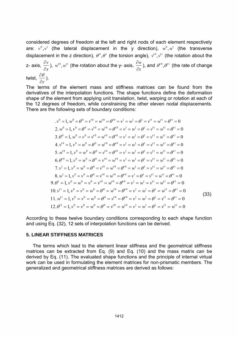
considered degrees of freedom at the left and right nods of each element respectively are: 10 ,vv (the lateral displacement in the y direction), 10 ,ww (the transverse displacement in the z direction), 10 , (the torsion angle), 10 ,vv (the rotation about the

z- axis, xv

), 10 , ww (the rotation about the y- axis, xw

), and 10 , (the rate of change

twist, x

).

The terms of the element mass and stiffness matrices can be found from the derivatives of the interpolation functions. The shape functions define the deformation shape of the element from applying unit translation, twist, warping or rotation at each of the 12 degrees of freedom, while constraining the other eleven nodal displacements. There are the following sets of boundary conditions:

0 ,1 .80 ,1 .70 ,1 .60 ,1 .50 ,1 .40 ,1 .30 ,1 .2

0 ,1 .

111110000001

111110000001

111111000000

111111000000

111111000000

111111000000

111111000000

111111000000

wvvwvvvwwvwwvwvvwvwvwvwvwvwvvwvwwvwvwwvvwvwvwvvwwvwvwvvw

wvwvwvwv

0 ,1 .120 ,1 .110 ,1 .10

0 ,1 .9

111110000001

111110000001

111110000001

111110000001

wvwvwvwvvvwvvwvvwwwvwwvvv

wvwvwvvwv

(33)

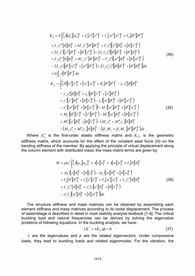
According to these twelve boundary conditions corresponding to each shape function and using Eq. (32), 12 sets of interpolation functions can be derived. 5. LINEAR STIFFNESS MATRICES The terms which lead to the element linear stiffness and the geometrical stiffness matrices can be extracted from Eq. (9) and Eq. (10) and the mass matrix can be derived by Eq. (11). The evaluated shape functions and the principle of internal virtual work can be used in formulating the element matrices for non-prismatic members. The generalized and geometrical stiffness matrices are derived as follows:

1412

22

4

22

4

22

22

000

dxJG

dxyyIwwyI

wwyIyIyI

zzIvvzI

vvzIzIzI

IwwIvvIuuAEK

L

T

TTccy

TTcy

TTcy

Tcy

Tcy

TTccz

TTcz

TTcz

Tcz

Tcz

L

TTy

Tz

T

(34)

dxMMzMzM

yMyMvvM

wwMvvM

wwMwwy

wwyvvz

vvzyy

zzRwwvvNK

Tyzzy

Tcycy

Tczcz

TTy

TTz

TTy

TTz

TTc

TTc

TTc

TTc

Tcc

lT

ccT

cTT

G

0

(35)

Where 0ijK is the first-order elastic stiffness matrix and ijGK is the geometric

stiffness matrix, which accounts for the effect of the constant axial force (N) on the bending stiffness of the member. By applying the principle of virtual displacement along the column element with distributed mass, the mass matrix terms are given by:

dxwθθwIy

vθθvIzθθyI

θθzIwwIvvIθθI

wθθwAyvθθvAz

θθIwwAvvAuuAωM

TTyc

TTzc

Tcy

Tcz

Ty

Tz

T

TTc

TTc

lT

sTTT

2

2

000

2

(36)

The structure stiffness and mass matrices can be obtained by assembling each element stiffness and mass matrices according to its nodal displacement. The process of assemblage is described in detail in most stability analysis textbook [1-4]. The critical buckling load and natural frequencies can be derived by solving the eigenvalue problems of following equations. In the buckling analysis, we have:

0)( * GKK (37)

are the eigenvalues and are the related eigenvectors. Under compressive loads, they lead to buckling loads and related eigenmodes. For the vibration, the

1413

eigenvalue problem is put:

0)( * MK (38)

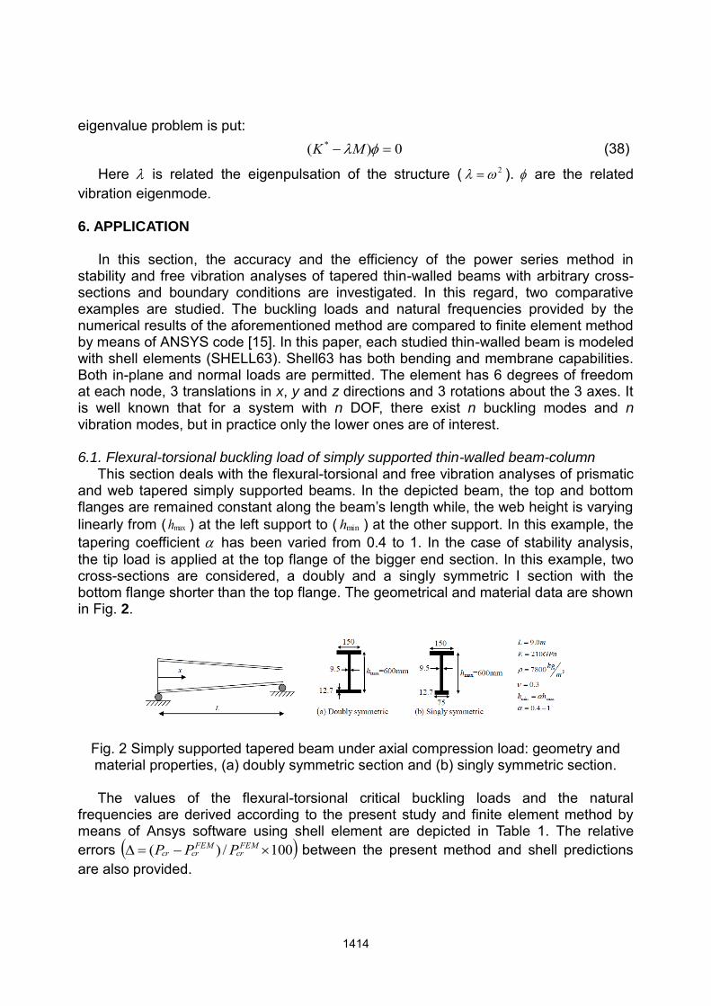
Here is related the eigenpulsation of the structure ( 2 ). are the related vibration eigenmode. 6. APPLICATION In this section, the accuracy and the efficiency of the power series method in stability and free vibration analyses of tapered thin-walled beams with arbitrary cross-sections and boundary conditions are investigated. In this regard, two comparative examples are studied. The buckling loads and natural frequencies provided by the numerical results of the aforementioned method are compared to finite element method by means of ANSYS code [15]. In this paper, each studied thin-walled beam is modeled with shell elements (SHELL63). Shell63 has both bending and membrane capabilities. Both in-plane and normal loads are permitted. The element has 6 degrees of freedom at each node, 3 translations in x, y and z directions and 3 rotations about the 3 axes. It is well known that for a system with n DOF, there exist n buckling modes and n vibration modes, but in practice only the lower ones are of interest. 6.1. Flexural-torsional buckling load of simply supported thin-walled beam-column This section deals with the flexural-torsional and free vibration analyses of prismatic and web tapered simply supported beams. In the depicted beam, the top and bottom flanges are remained constant along the beam’s length while, the web height is varying linearly from ( maxh ) at the left support to ( minh ) at the other support. In this example, the tapering coefficient has been varied from 0.4 to 1. In the case of stability analysis, the tip load is applied at the top flange of the bigger end section. In this example, two cross-sections are considered, a doubly and a singly symmetric I section with the bottom flange shorter than the top flange. The geometrical and material data are shown in Fig. 2.

Fig. 2 Simply supported tapered beam under axial compression load: geometry and material properties, (a) doubly symmetric section and (b) singly symmetric section.

The values of the flexural-torsional critical buckling loads and the natural frequencies are derived according to the present study and finite element method by means of Ansys software using shell element are depicted in Table 1. The relative errors 100/)( FEM

crFEM

crcr PPP between the present method and shell predictions are also provided.

1414

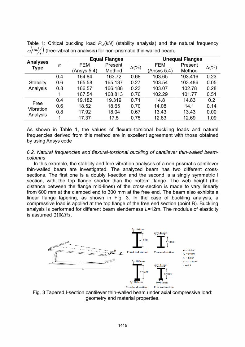
Table 1: Critical buckling load Pcr(kN) (stability analysis) and the natural frequency srad (free-vibration analysis) for non-prismatic thin-walled beam.

Analyses Type

Equal Flanges Unequal Flanges

FEM (Ansys 5.4)

Present Method

(%) FEM (Ansys 5.4)

Present Method

(%)

Stability Analysis

0.4 164.84 163.72 0.68 103.65 103.416 0.23 0.6 165.58 165.137 0.27 103.54 103.486 0.05 0.8 166.57 166.188 0.23 103.07 102.78 0.28 1 167.54 168.813 0.76 102.29 101.77 0.51

Free Vibration Analysis

0.4 19.182 19.319 0.71 14.8 14.83 0.2 0.6 18.52 18.65 0.70 14.08 14.1 0.14 0.8 17.92 18.04 0.67 13.43 13.43 0.00 1 17.37 17.5 0.75 12.83 12.69 1.09

As shown in Table 1, the values of flexural-torsional buckling loads and natural frequencies derived from this method are in excellent agreement with those obtained by using Ansys code 6.2. Natural frequencies and flexural-torsional buckling of cantilever thin-walled beam-columns In this example, the stability and free vibration analyses of a non-prismatic cantilever thin-walled beam are investigated. The analyzed beam has two different cross-sections. The first one is a doubly I-section and the second is a singly symmetric I section, with the top flange shorter than the bottom flange. The web height (the distance between the flange mid-lines) of the cross-section is made to vary linearly from 600 mm at the clamped end to 300 mm at the free end. The beam also exhibits a linear flange tapering, as shown in Fig. 3. In the case of buckling analysis, a compressive load is applied at the top flange of the free end section (point B). Buckling analysis is performed for different beam slenderness L=12m. The modulus of elasticity is assumed GPa210 .

Fig. 3 Tapered I-section cantilever thin-walled beam under axial compressive load:

geometry and material properties.

1415

Table 2 presents the variation of the flexural-torsional buckling loads of the cantilever column with non-uniform cross-section computed by the proposed procedure and compared to those obtained by finite element method using Ansys software. Table 2: Critical buckling load Pcr(kN) for the non-prismatic beams. (Example 2)

L(m)

Mode

FTB of cantilever beam (KN), load on top flange

Equal Flanges Unequal Flanges

FEM (Ansys 5.4)

Present Method

(%) FEM (Ansys 5.4)

Present Method

(%)

12 n=1 27.562 27.494 0.25 16.32 16.38 0.37 n=2 188.02 188.032 0.01 129.04 123.66 4.17

7. CONCLUSIONS The total potential energy principle considering the effects of strain and initial stress, the kinematic energy and the work of the applied loads is used to derive the equilibrium equations of motion of thin-walled beams. Then, power series expansions method is used to derive the exact shape functions for the element with 12 degrees of freedom. Then, the stiffness and mass matrices are derived. The proposed method can be applied in various form of non-prismatic member under axially concentrated loads and variable mass per unit length. Furthermore; it can be used to evaluate both natural frequency and buckling load concurrently.

REFERENCES Al-Sadder S.Z. (2004), “Exact expression for stability functions of a general non-

prismatic beam-column member”. Journal of Constructional Steel Research, Vol. 60, 1561-84.

Andrade A, Camotim D, Borges Dinis P. (2007), “Lateral-torsional buckling of singly

symmetric web-tapered thin-walled I-beams, 1D model vs. shell FEA”. Computers and Structures, Vol. 85, 1343–1359.

Asgarian B, Soltani M, Mohri F. (2013), “Lateral-torsional buckling of tapered thin-walled beams with arbitrary cross-sections”. Thin-Walled Structures, Vol. 62, 96-108.

Chen C-N. (2000), “Dynamic equilibrium of non-prismatic beams defined on an arbitrarily selected co-ordinate system”. Journal of Sound and vibration, Vol. 230(2), 241-260.

Eisenberger M. (1994), “Vibration frequencies for beams on variable one- and two-parameters elastic foundation”. Journal of sound and vibration, Vol. 176(5), 577-584.

Eisenberger M and Cohen R. (1995), “Flexural-torsional buckling of variable and open cross-section members”. Journal of Engineering Mechanics, ASCE, Vol. 121(2), 244-254.

Kim S-B, Kim M-Y. (2000), “Improved formulation for spatial stability and free vibration of thin-walled tapered beams and space frames”. Engineering Structures, Vol. 22,

1416

446–458. Ronagh HR, Bradford MA and Attard MM. (2000), “Non-linear analysis of thin-walled

members of variable cross-section. Part I: Theory”. Computers and Structures, Vol. 77, 285-299.

Ronagh HR, Bradford MA and Attard MM. (2000), “Non-linear analysis of thin-walled members of variable cross-section. Part II: Application”. Computers and Structures, Vol. 77, 301-313.

Yang YB, Yau JD. (1987), “Stability of beams with tapered I-sections”. Journal of Engineering Mechanics, ASCE, Vol. 113(9), 1337–1357.

Timoshenko SP, Gere JM. (1961), Theory of elastic stability, 2nd ed. New York: McGraw-Hill.

Vlasov VZ. (1959), Thin-walled elastic beams, Moscow, French translation, Pièces longues en voiles minces, Eyrolles, Paris, 1962.

Chen WF, Lui EM. (1987), Structural stability, theory and implementation, New York, Elsevier.

Bazant ZP, Cedolin L. (1991), Stability of structures Elastic, inelastic fracture and damage theories, New York, Dover Publications.

MATLAB Version 7.6 .MathWorks Inc, USA, 2008. ANSYS, Version 5.4, Swanson Analysis System, Inc, 2007.

1417