Embed Size (px)
Citation preview
Application of the Finite Element Method to
Slope Stability
Rocscience Inc. Toronto, 2001-2004
This document outlines the capabilities of the finite element method in the analysis of slope stability problems. The manuscript describes the constitutive laws of material behaviour such as the Mohr-Coulomb failure criterion, and material properties input parameters, required to adequately model slope failure. It also discusses advanced topics such as strength reduction techniques and the definition of slope collapse. Several slopes are analyzed with the finite element method, and the results compared with outcomes from various limit equilibrium methods. Conclusions for the practical use of the finite element method are also given.
1. Introduction
Slope stability analysis is an important area in geotechnical engineering. Most textbooks on soil
mechanics include several methods of slope stability analysis. A detailed review of equilibrium
methods of slope stability analysis is presented by Duncan (Duncan, 1996). These methods
include the ordinary method of slices, Bishop’s modified method, force equilibrium methods,
Janbu’s generalized procedure of Slices, Morgenstern and Price’s method and Spencer’s method.
These methods, in general, require the soil mass to be divided into slices. The directions of the
forces acting on each slice in the slope are assumed. This assumption is a key role in
distinguishing one limit equilibrium method from another.
Limit equilibrium methods require a continuous surface passes the soil mass. This surface is
essential in calculating the minimum factor of safety (FOS) against sliding or shear failure.
Before the calculation of slope stability in these methods, some assumptions, for example, the
side forces and their directions, have to be given out artificially in order to build the equations of
equilibrium.
With the development of cheaper personal computer, finite element method has been
increasingly used in slope stability analysis. The advantage of a finite element approach in the
analysis of slope stability problems over traditional limit equilibrium methods is that no
1
assumption needs to be made in advance about the shape or location of the failure surface, slice
side forces and their directions. The method can be applied with complex slope configurations
and soil deposits in two or three dimensions to model virtually all types of mechanisms. General
soil material models that include Mohr-Coulomb and numerous others can be employed. The
equilibrium stresses, strains, and the associated shear strengths in the soil mass can be computed
very accurately. The critical failure mechanism developed can be extremely general and need not
be simple circular or logarithmic spiral arcs. The method can be extended to account for seepage
induced failures, brittle soil behaviors, random field soil properties, and engineering
interventions such as geo-textiles, soil nailing, drains and retaining walls (Swan et al, 1999). This
method can give information about the deformations at working stress levels and is able to
monitor progressive failure including overall shear failure (Griffiths, 1999).
Generally, there are two approaches to analyze slope stability using finite element method. One
approach is to increase the gravity load and the second approach is to reduce the strength
characteristics of the soil mass.
Phase2 has been widely used in geotechnical and mining engineering as a tool for the design and
the analysis of tunnel, surface excavation and ore extraction and supports (Phase2, 1999).
However, few applications have been reported in the area of slope stability analysis. Obviously,
its potential applications in the most of areas in geotechnical engineering will be shown with
time passing and the accumulation of users’ experience.
This manuscript is prepared to validate the applicability of using the finite element program
Phase2, in the analysis of slope stability problems. Four slope stability examples are presented
and compared to previous FEM work and limit equilibrium methods (Griffiths, 1999 and Slide)
2. Important aspects in slope stability analysis
In this section, three major aspects that influence slope stability analysis are discussed. The first
is about the material properties of the slope model. The second is the influence of calculating
factor of safety to slope stability and the third aspect is the definition of the slope failure.
2
i) Model material properties
This work applied only for two-dimensional plain-strain problems. The Mohr-Coulomb
constitutive model used to describe the soil (or rock) material properties. The Mohr-Coulomb
criterion relates the shear strength of the material to the cohesion, normal stress and angle of
internal friction of the material. The failure surface of the Mohr-Coulomb model can be
presented as:
12
1sin cos sin sin cos3 3If J Cφ φ φ = + Θ − Θ −
(1)
where φ is the angle of internal friction, C is cohesion and
I1 1 2 3( ) m3σ σ σ σ= + + = (2)
( )2 2 2 2 2 22
12 x y z xy yz zxJ s s s τ τ τ= + + + + +
(3)
3
2
1 3
2
3 31sin3 2
JJ
− Θ =
(4)
where J s 2 23 2x y z xy yz zx x yz y xz z xys s s s sτ τ τ τ τ τ= + − − − 2
, , x x m y y m z zs s sσ σ σ σ σ= − = − = − mσand
For Mohr-Coulomb material model, six material properties are required. These properties are the
friction angle φ, cohesion C, dilation angle ψ, Young’s modulus E, Poisson’s ratio ν and unit
weight of soil γ. Young’s modulus and Poisson’s ratio have a profound influence on the
computed deformations prior to slope failure, but they have little influence on the predicted
factor of safety in slope stability analysis. Thus in this work two constant values for these
parameters are used throughout the examples (E = 105 kN/m2 and ν = 0.3).
Dilation angle, ψ affects directly the volume change during soil yielding. If ψ = φ, the plasticity
flow rule is known as “associated”, and if ψ ≠ φ, the plasticity flow rule is considered as “no-
associated”. The change in the volume during the failure is not considered in this study and
therefore the dilation angle is taken as 0. Therefore, only three parameters (friction angle,
cohesion and unit weight of material) of the model material are considered in the modeling of
slope failure.
3
ii) Factor of Safety (FOS) and Strength Reduction Factor (SRF).
Slope fails because of its material shear strength on the sliding surface is insufficient to resist the
actual shear stresses. Factor of safety is a value that is used to examine the stability state of
slopes. For FOS values greater than 1 means the slope is stable, while values lower that 1 means
slope is instable. In accordance to the shear failure, the factor of safety against slope failure is
simply calculated as:
f
FOSττ
= (5)
Where τ is the shear strength of the slope material, which is calculated through Mohr-Coulomb
criterion as:
φστ tannC += (6)
and fτ is the shear stress on the sliding surface. It can be calculated as:
fnff C φστ tan+= (7)
where the factored shear strength parameters and fC fφ are:
SRF
CC f = (8)
)tan(tan 1
SRFFφφ −= (9)
Where SRF is strength reduction factor. This method has been referred to as the ‘shear strength
reduction method’. To achieve the correct SRF, it is essential to trace the value of FOS that will
just cause the slope to fail.
iii) Slope Collapse
Non-convergence within a user-specified number of iteration in finite element program is taken
as a suitable indicator of slope failure. This actually means that no stress distribution can be
achieved to satisfy both the Mohr-Coulomb criterion and global equilibrium. Slope failure and
numerical non-convergence take place at the same time and are joined by an increase in the
4
displacements. Usually, value of the maximum nodal displacement just after slope failure has a
big jump compared to the one before failure.
3. Slope stability benchmark example To assess the accuracy of the proposed algorithm using Phase2, simulations were performed for
some specific parameters. The studied parameters include finite element type, maximum number
of iterations and convergence factor, and the searching method for SRF.
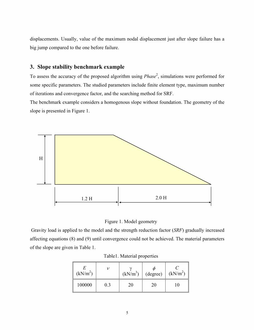
The benchmark example considers a homogenous slope without foundation. The geometry of the
slope is presented in Figure 1.
Figure 1. Model geometry
Gravity load is applied to the model and the strength reduction factor (SRF) gradually increased
affecting equations (8) and (9) until convergence could not be achieved. The material parameters
of the slope are given in Table 1.
Table1. Material properties
E (kN/m2)
ν γ (kN/m3)
φ (degree)
C (kN/m2)
100000 0.3 20 20 10
2.0 H 1.2 H
H
5
The first parameter studied in this example is the effect of different element types to the accuracy
of the results Phase2 comes with four element types: 3 nodded triangle (T3), 6 nodded triangle
(T6), 4 nodded quadrilateral (Q4) and 8 nodded quadrilateral (Q8). Two different meshes are
used to discretize the slope geometry. The first mesh uses 1408 triangular elements. The second
mesh is discretized with 104 elements. Results of the factor of safety for different element types
are presented with comparison to Bishop’s method and Griffith’s FE result in Table 2.
Table 2. Factor of safety using different element types
Phase2 Bishop Griffiths
T3 T6 Q4 Q8
1.38 1.4 1.51 1.39 1.47 1.42
From table 2, the differences of the factor of safety using T3 and Q4 are larger than 5%, while
the factors of safety using T6 and Q8 are close to Griffiths’ and Bishop’s results. Hence T6 and
Q8 are used for the verification examples presented in the following sections.
The second parameter studied in this section is the effect of tolerance and number of iteration on
the factor of safety. Phase2 uses a default value of 500 to the maximum number of iteration and a
default value of 0.001 for the tolerance. Two values of maximum number of iteration are
considered, 500 and 1000. Results from both cases were very close. For tolerance value, couple
of values is assumed and the tolerance of 0.005 is chosen as an indicator.
The third parameter is the searching procedure. In this work, the procedure used to determine the
strength reduction factor is
2
121
−−−
−±= nn
nn
SRFSRFSRFSRF (9)
6
Equation (9) determines whether to increase or decrease the value of SRF in the next FOS.
4. Examples of slope stability analysis
As it is indicated in the previous section, two meshes will be considered in all the examples in
this section. These meshes use T6 and Q8 elements.
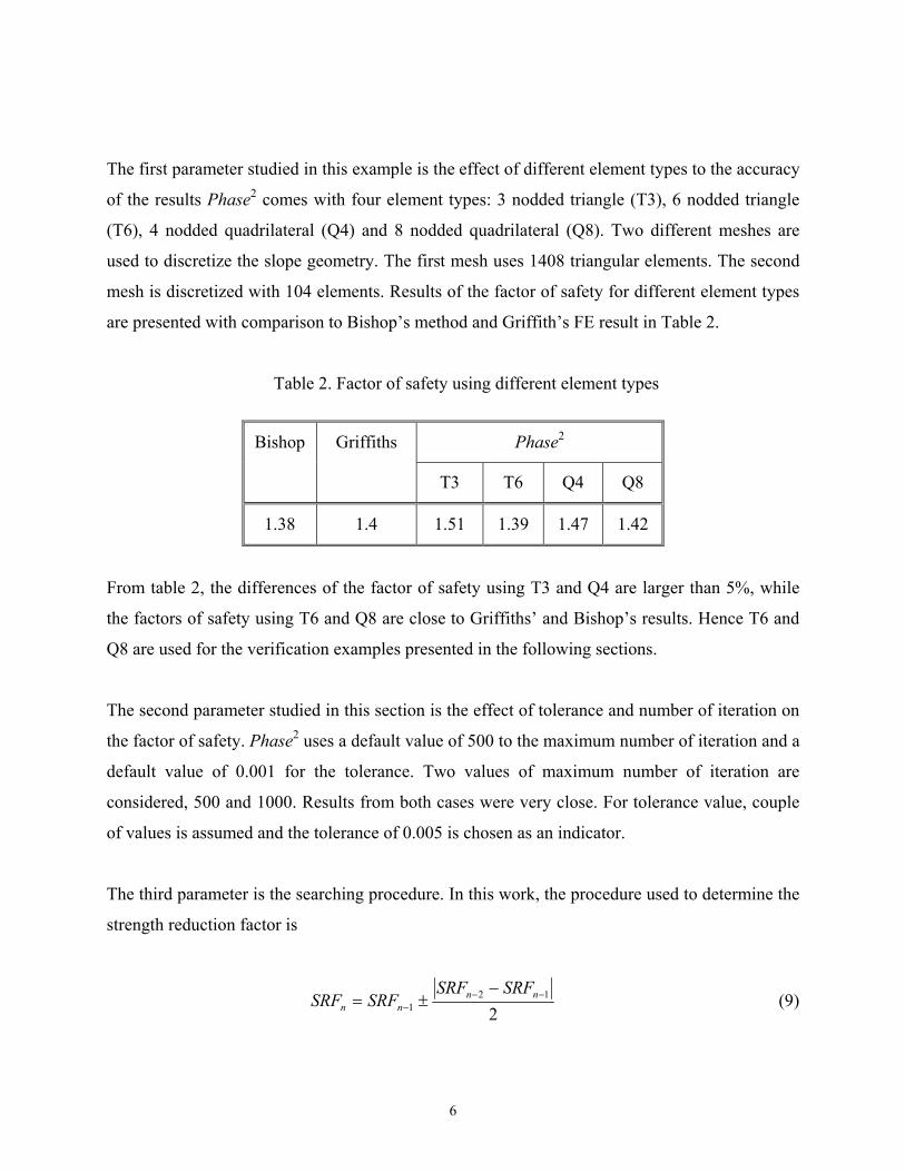
Example 1. Homogeneous Slope with a Foundation Layer. This problem is taken from the verification manual of Slide 3.0 (verification #1). Without
considering pore water pressure, there is a homogeneous slope with a foundation layer. The slope
model geometry is presented in Figure 2. The slope material properties are shown in table 3.
Figure 2. Slope model geometry
Table 3. Slope material properties
E (kN/m2)
ν γ (kN/m3)
φ (degree)
C (kN/m2)
100000 0.3 20.2 19.6 3.0
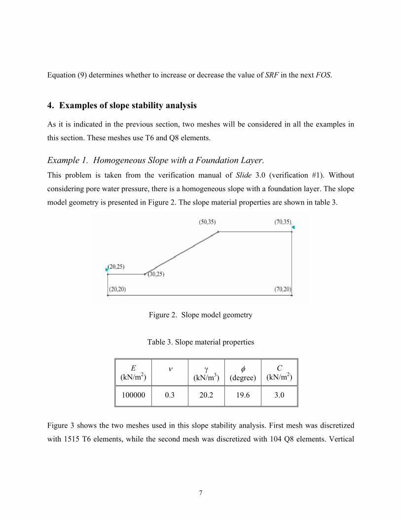
Figure 3 shows the two meshes used in this slope stability analysis. First mesh was discretized
with 1515 T6 elements, while the second mesh was discretized with 104 Q8 elements. Vertical
7
rollers are used on the left and the right side of the geometry boundaries and full fixity at the
bottoms of the geometry.
(a) Mesh with T6 elements
(b) Mesh with Q8 elements
Figure 3. Undeformed mesh
8
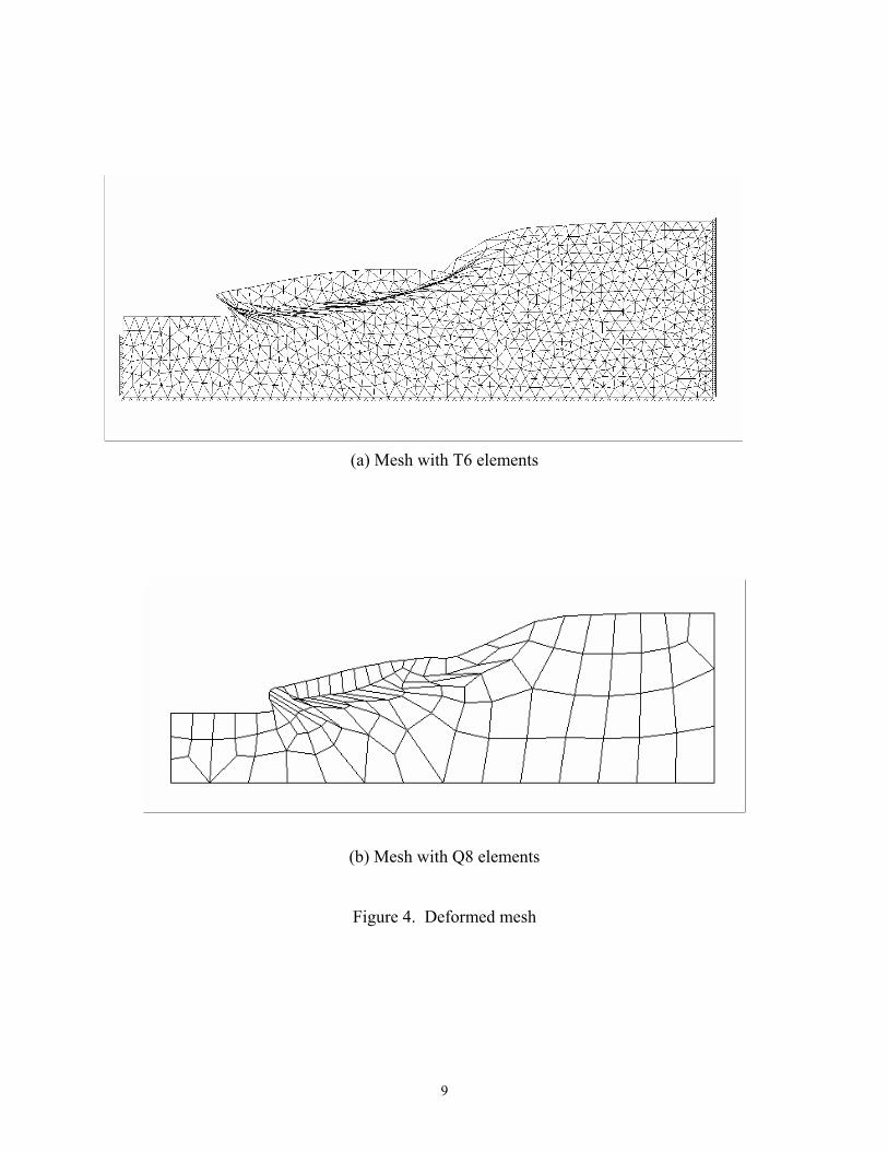
(a) Mesh with T6 elements
(b) Mesh with Q8 elements
Figure 4. Deformed mesh
9
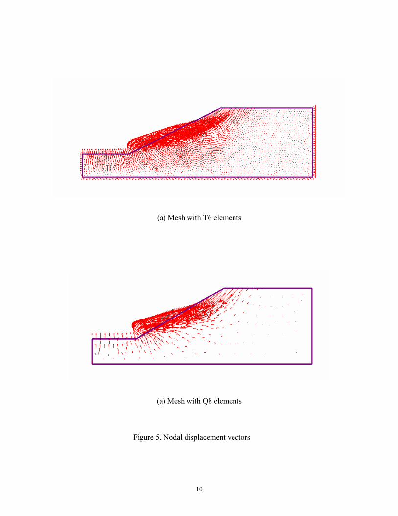
(a) Mesh with T6 elements
(a) Mesh with Q8 elements
Figure 5. Nodal displacement vectors
10
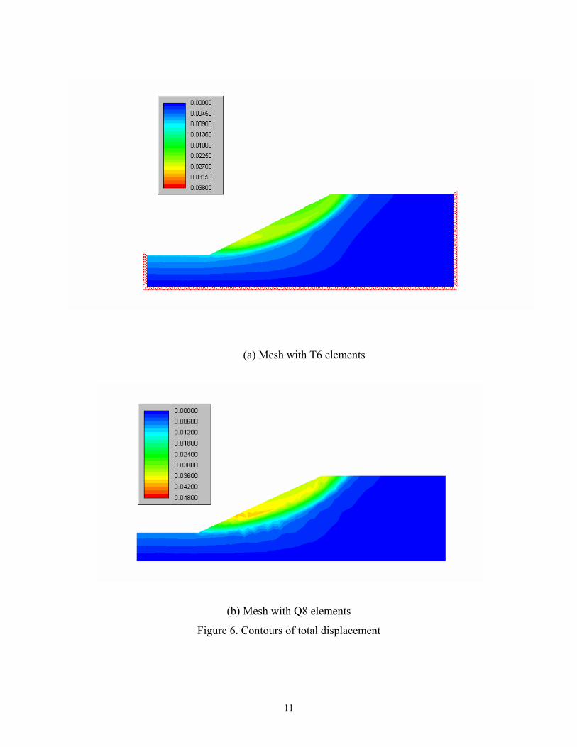
(a) Mesh with T6 elements
(b) Mesh with Q8 elements
Figure 6. Contours of total displacement
11
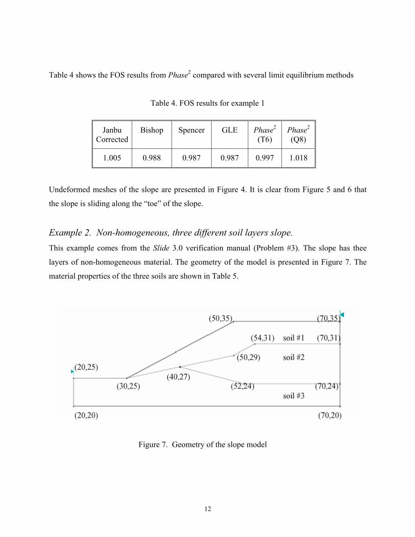
Table 4 shows the FOS results from Phase2 compared with several limit equilibrium methods
Table 4. FOS results for example 1
Janbu Corrected
Bishop Spencer GLE Phase2 (T6)
Phase2 (Q8)
1.005 0.988 0.987 0.987 0.997 1.018
Undeformed meshes of the slope are presented in Figure 4. It is clear from Figure 5 and 6 that
the slope is sliding along the “toe” of the slope.
Example 2. Non-homogeneous, three different soil layers slope. This example comes from the Slide 3.0 verification manual (Problem #3). The slope has thee
layers of non-homogeneous material. The geometry of the model is presented in Figure 7. The
material properties of the three soils are shown in Table 5.
Figure 7. Geometry of the slope model
12
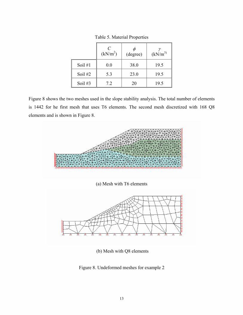
Table 5. Material Properties
C (kN/m2)
φ (degree)
γ (kN/m3)
Soil #1 0.0 38.0 19.5
Soil #2 5.3 23.0 19.5
Soil #3 7.2 20 19.5
Figure 8 shows the two meshes used in the slope stability analysis. The total number of elements
is 1442 for he first mesh that uses T6 elements. The second mesh discretized with 168 Q8
elements and is shown in Figure 8.
(a) Mesh with T6 elements
(b) Mesh with Q8 elements
Figure 8. Undeformed meshes for example 2
13
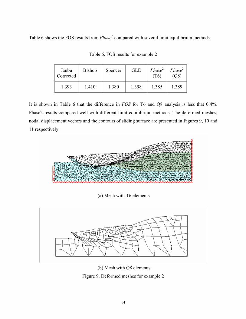
Table 6 shows the FOS results from Phase2 compared with several limit equilibrium methods
Table 6. FOS results for example 2
Janbu Corrected
Bishop Spencer GLE Phase2 (T6)
Phase2 (Q8)
1.393 1.410 1.380 1.398 1.385 1.389
It is shown in Table 6 that the difference in FOS for T6 and Q8 analysis is less that 0.4%.
Phase2 results compared well with different limit equilibrium methods. The deformed meshes,
nodal displacement vectors and the contours of sliding surface are presented in Figures 9, 10 and
11 respectively.
(a) Mesh with T6 elements
(b) Mesh with Q8 elements
Figure 9. Deformed meshes for example 2
14
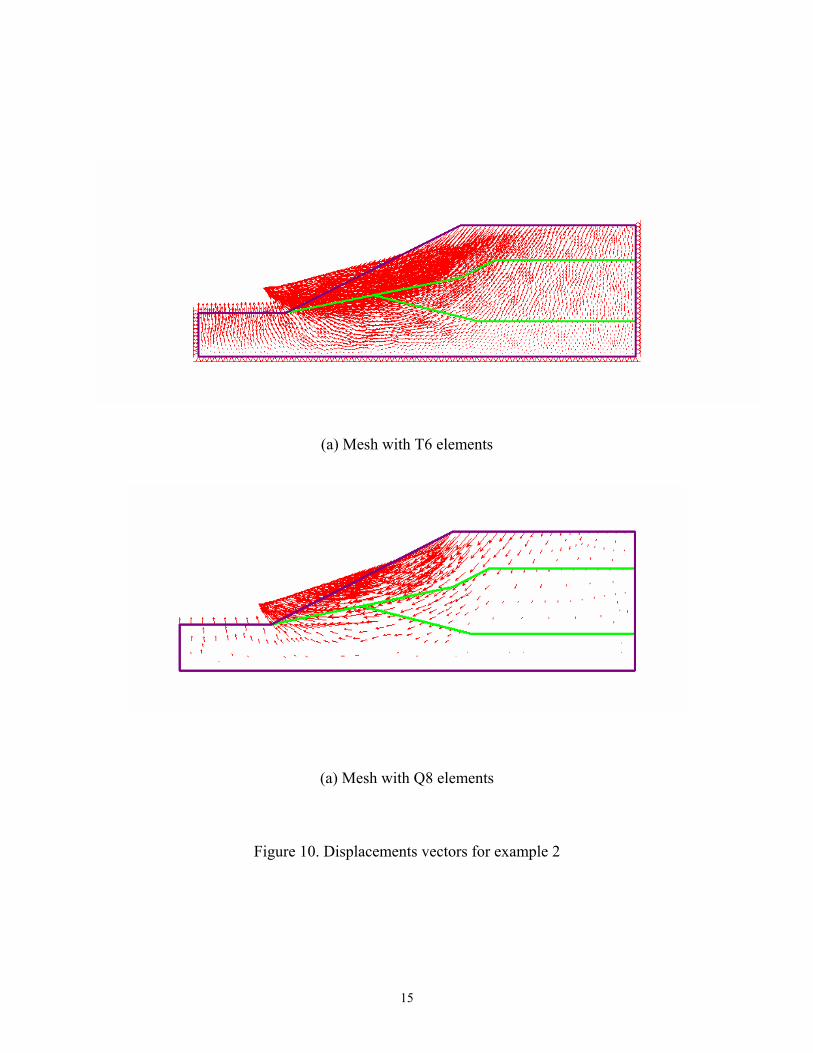
(a) Mesh with T6 elements
(a) Mesh with Q8 elements
Figure 10. Displacements vectors for example 2
15
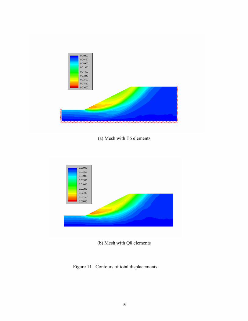
(a) Mesh with T6 elements
(b) Mesh with Q8 elements
Figure 11. Contours of total displacements
16

Example 3. An undrained clay slope failure with a thin weak layer This example demonstrates a stability analysis of a slope of undrained clay. This example is
taken from Griffiths’ paper (Griffiths, 1999). The slope model consists of a thin layer of week
material. The weak layer runs parallel to the slope and then turns to be horizontal in the toe zone.
The presence of this thin weak layer in the slope influences the stability of slope. In this
example, different values of Cu2/Cu1 was considered.
Figure 12. Undrained clay slope with a foundation layer including a thin weak
The geometry of the slope model is presented in Figure 12. The slope height is 10 meters and
Cu1/γH ratio is taken as 0.25. Table 7 presents the material properties for the slope model.
Table 7. Slope material properties
Cu1 (kN/m2)
φ (degree)
γ (kN/m3)
Cu2 (Cu2/Cu1=0.6)
Cu2 (Cu2/Cu1=1)
Cu2 (Cu2/Cu1=0.2)
0.05 0.0 20.0 0.05 0.03 0.01
17
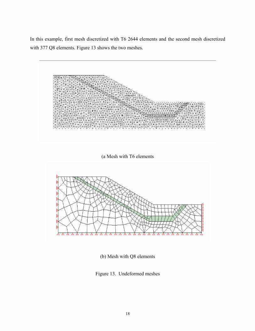
In this example, first mesh discretized with T6 2644 elements and the second mesh discretized
with 377 Q8 elements. Figure 13 shows the two meshes.
(a Mesh with T6 elements
(b) Mesh with Q8 elements
Figure 13. Undeformed meshes
18

Case 1: Cu2/Cu1=1
(a) Mesh with T6 elements (FOS=1.45)
(b) Mesh with Q8 elements (FOS=1.47)
Figure 14. Deformed meshes
19
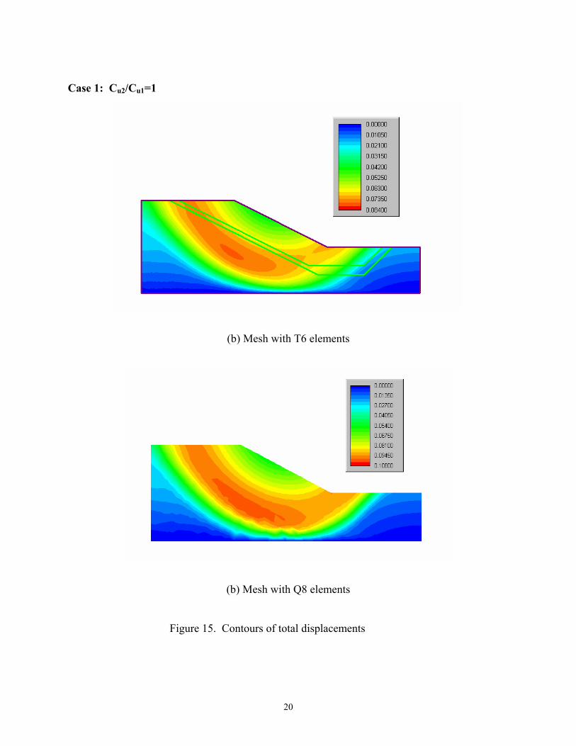
Case 1: Cu2/Cu1=1
(b) Mesh with T6 elements
(b) Mesh with Q8 elements
Figure 15. Contours of total displacements
20
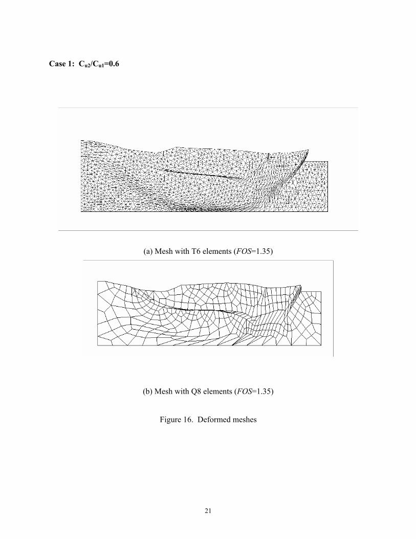
Case 1: Cu2/Cu1=0.6
(a) Mesh with T6 elements (FOS=1.35)
(b) Mesh with Q8 elements (FOS=1.35)
Figure 16. Deformed meshes
21
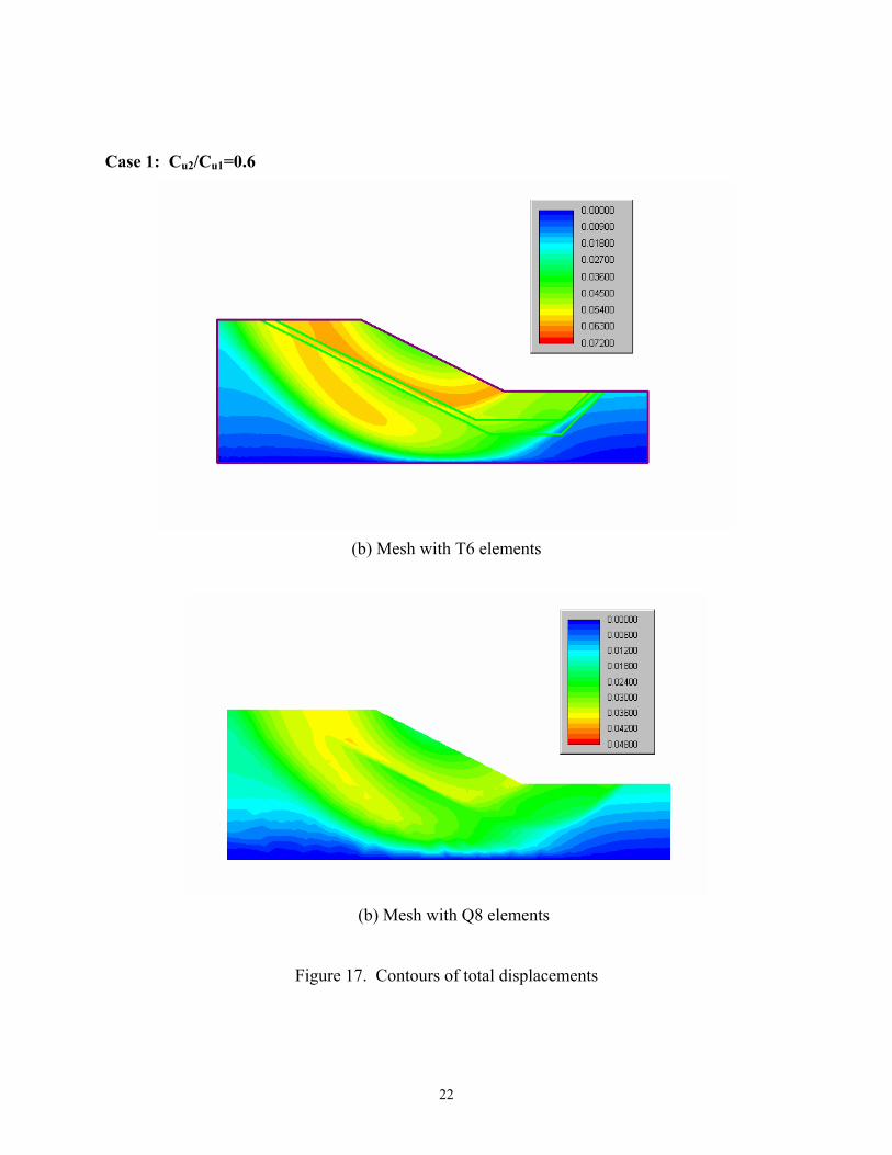
Case 1: Cu2/Cu1=0.6
(b) Mesh with T6 elements
(b) Mesh with Q8 elements
Figure 17. Contours of total displacements
22
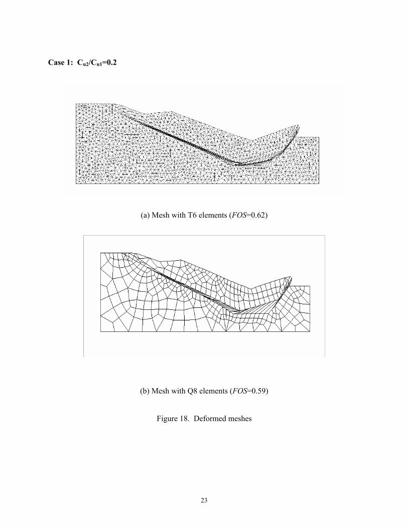
Case 1: Cu2/Cu1=0.2
(a) Mesh with T6 elements (FOS=0.62)
(b) Mesh with Q8 elements (FOS=0.59)
Figure 18. Deformed meshes
23
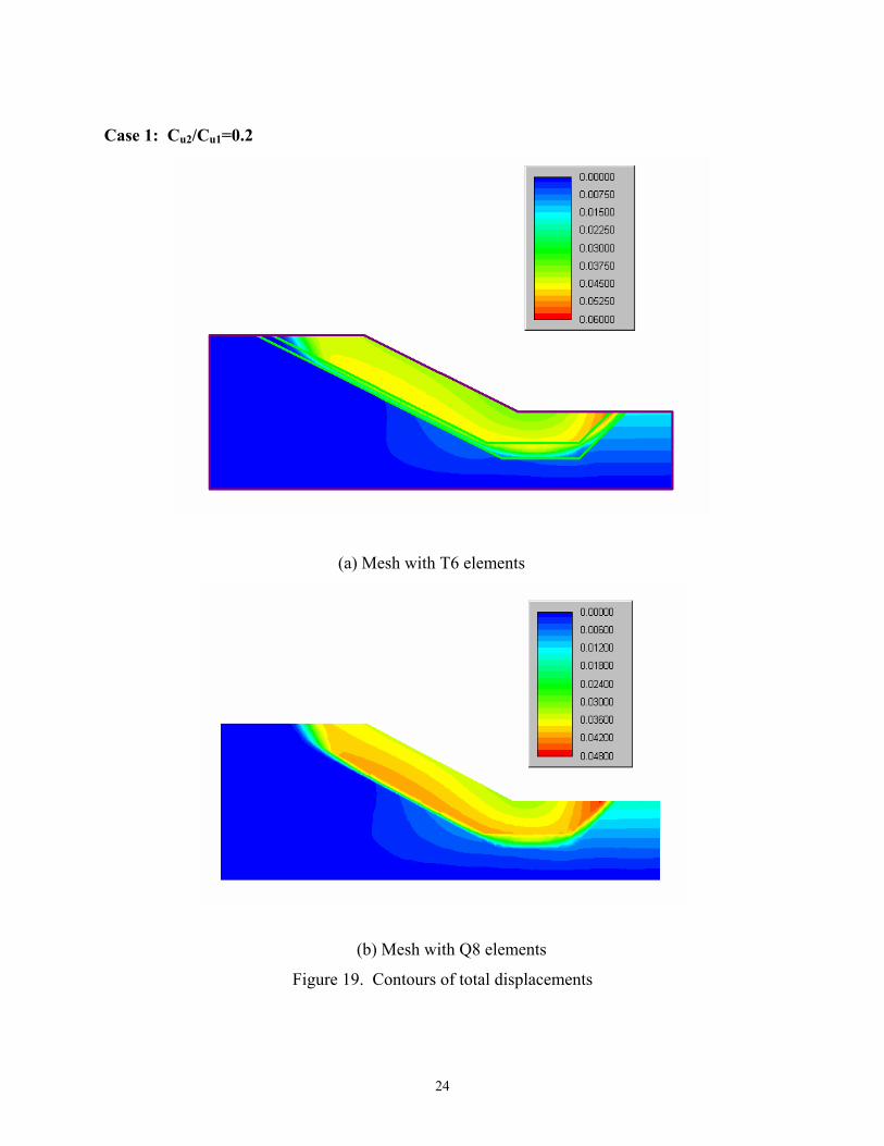
Case 1: Cu2/Cu1=0.2
(a) Mesh with T6 elements
(b) Mesh with Q8 elements
Figure 19. Contours of total displacements
24

Cu2/Cu1
Figure 20. FOS for different values of Cu2/Cu1 (Griffiths, 1999)
2
0
0.2
0.4
0.6
0.8
1
1.2
1.4
1.6
1.8
0 0.2 0.4 0.6 0.8 1 1.2
Cu2/Cu1
FOS
Phase2base circlethree line wedge
Taylor (1937) FOS=1.47
Taylor (1937) FOS=1.47
0
0.2
0.4
0.6
0.8
1
1.2
1.4
1.6
1.8
2
0 0.2 0.4 0.6 0.8 1 1.2
Cu2/Cu1
FOS
base circlethree line wedgePhase2_8nq
Taylor (1937) FOS=1.47
(a) T6 elements (b) Q8 elements
Figure 21. FOS for different values of Cu2/Cu1 from Phase2
25
Seven cases are studied in this example using T6 and Q8 elements. Three cases used different
cohesion strength ratio for the thin layer compared to the slope material. These ratios were 0.2,
0.6 and 1.0. Figures 14-19 show the deformed meshes and the total displacements contours for
the two meshes.
Figures 20-21 shows three results obtained using finite element analysis and Janbu’s method
assuming both circular (base failure) and three line wedge mechanism following the path of
weak layer. Phase2 results are compared well with Griffiths’ FE results as it is shown in Figures
20-21. For the homogeneous slope model (Cu1/Cu2=1.0), FOS was close to the Taylor solution
(Taylor, 1937). The failure mechanism showed a circular slip which confirms the expectation.
For the case of Cu2/Cu1≈0.6, a distinct change is observed. It shows that for Cu2/Cu1>0.6, the base
failure mechanism governs the slope behaviors and the weaker thin layer doesn’t influence the
factor of safety. For Cu2/Cu1<0.6, the thin weak layer mechanism controls the slope behavior and
the FOS falls linearly. The obvious difference between Phase2 and Griffiths’ results is that the
point of distinct change moves to the position of Cu2/Cu1≈0.5. Figure 21 shows that both T6 and
Q8 are very similar.
The failure mechanisms of T6 and Q8 for Cu2/Cu1=0.2, Cu2/Cu1=0.6 and Cu2/Cu1=1.0 are shown in
Figure 14-19. For the case of Cu2/Cu1=0.2, figures 18-19 indicate a highly concentrated non-
circular mechanism moving along the path of the thin weak layer. The strength of the thin layer
is 60% of the surrounding soil. The sliding surface of the slope failure happens in the thin weak
layer and the circular failure (base failure). There failure mechanisms are same as those obtained
by Griffiths.
26
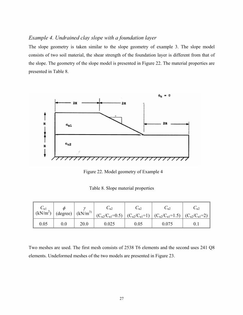
Example 4. Undrained clay slope with a foundation layer The slope geometry is taken similar to the slope geometry of example 3. The slope model
consists of two soil material, the shear strength of the foundation layer is different from that of
the slope. The geometry of the slope model is presented in Figure 22. The material properties are
presented in Table 8.
Figure 22. Model geometry of Example 4
Table 8. Slope material properties
Cu1 (kN/m2)
φ (degree)
γ (kN/m3)
Cu2 (Cu2/Cu1=0.5)
Cu2 (Cu2/Cu1=1)
Cu2 (Cu2/Cu1=1.5)
Cu2 (Cu2/Cu1=2)
0.05 0.0 20.0 0.025 0.05 0.075 0.1
Two meshes are used. The first mesh consists of 2538 T6 elements and the second uses 241 Q8
elements. Undeformed meshes of the two models are presented in Figure 23.
27
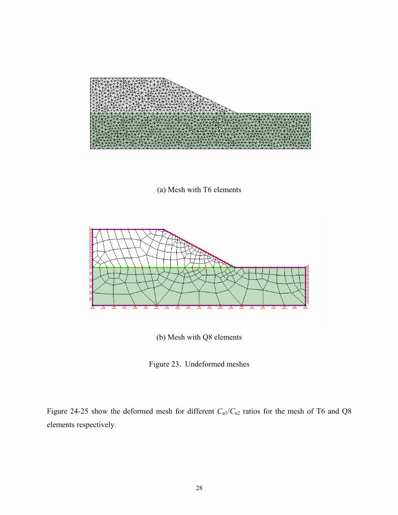
(a) Mesh with T6 elements
(b) Mesh with Q8 elements
Figure 23. Undeformed meshes
Figure 24-25 show the deformed mesh for different Cu1/Cu2 ratios for the mesh of T6 and Q8
elements respectively.
28
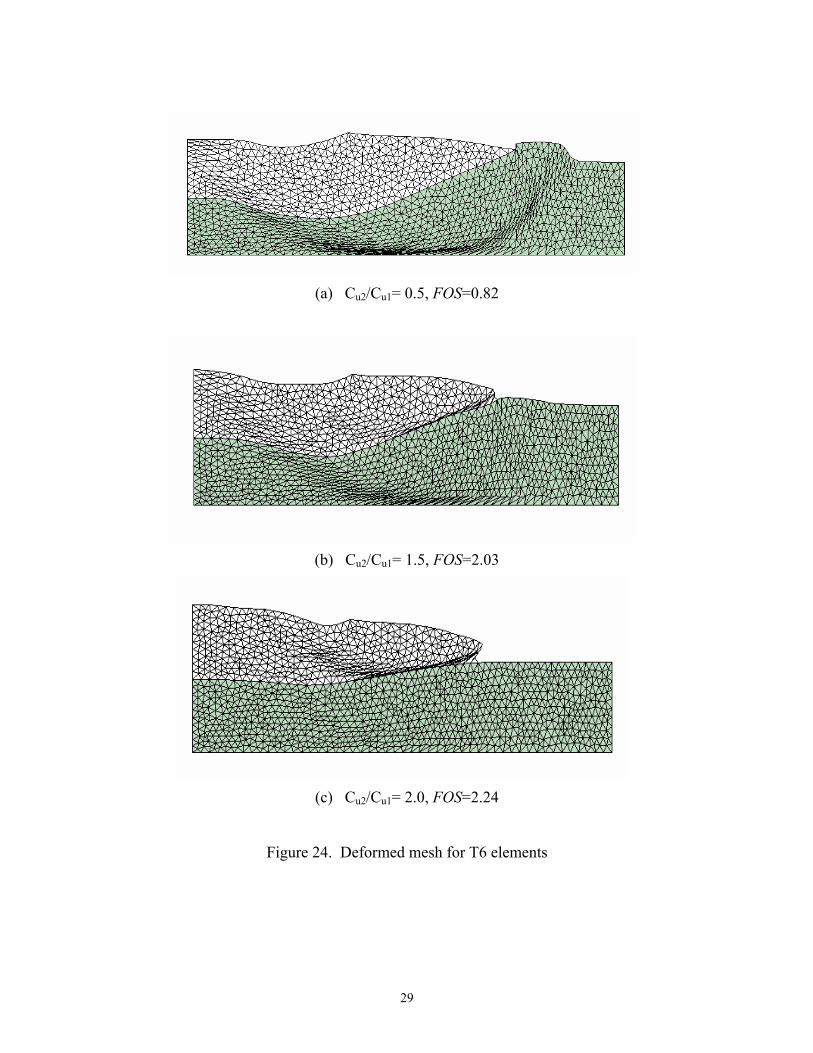
(a) Cu2/Cu1= 0.5, FOS=0.82
(b) Cu2/Cu1= 1.5, FOS=2.03
(c) Cu2/Cu1= 2.0, FOS=2.24
Figure 24. Deformed mesh for T6 elements
29
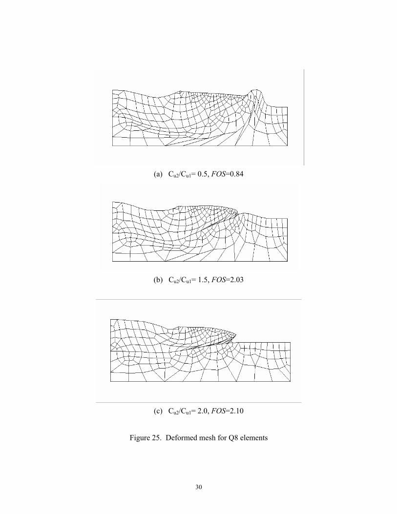
(a) Cu2/Cu1= 0.5, FOS=0.84
(b) Cu2/Cu1= 1.5, FOS=2.03
(c) Cu2/Cu1= 2.0, FOS=2.10
Figure 25. Deformed mesh for Q8 elements
30
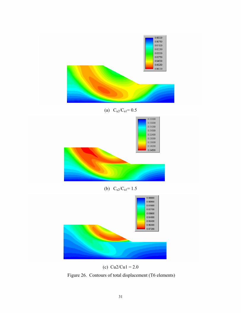
(a) Cu2/Cu1= 0.5
(b) Cu2/Cu1= 1.5
(c) Cu2/Cu1 = 2.0
Figure 26. Contours of total displacement (T6 elements)
31
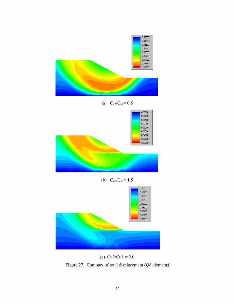
(a) Cu2/Cu1= 0.5
(b) Cu2/Cu1= 1.5
(c) Cu2/Cu1 = 2.0
Figure 27. Contours of total displacement (Q8 elements)
32
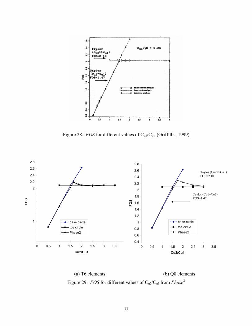
Figure 28. FOS for different values of Cu2/Cu1 (Griffiths, 1999)
1.8 1.6 1.4 1.2
0.8
0.6
0.4
1
2
2.2
2.4
2.6
2.8
0 0.5 1 1.5 2 2.5 3 3.5 4
Cu2/Cu1
FOS
base circle toe circlePhase2
0.4
0.6
0.8
1
1.2
1.4
1.6
1.8
2
2.2
2.4
2.6
2.8
0 0.5 1 1.5 2 2.5 3 3.5
Cu2/Cu1
FOS
base circle toe circlePhase2
Taylor (Cu1=Cu2) FOS=1.47
Taylor (Cu2>>Cu1) FOS=2.10
(a) T6 elements (b) Q8 elements
Figure 29. FOS for different values of Cu2/Cu1 from Phase2
33
Figures 24-27 show the deformed mesh and the total displacement contours for different slope
cases. It is clear from these figures that the values of Cu2/Cu1 will dominate the failure
mechanism. A deep-seated base failure mechanism is dominated when Cu2<<Cu1 while a shollow
‘toe’ faile mechanis is noticed for the case when Cu2>>Cu1. The deformed meshes compared well
with the results presented by Griffiths.
Figure 29 shows the variation of FOS verses different values of Cu2/Cu1 for the two meshes. It is
also plotted in Figure 29 the values of Taylor’s solution. Figure 29 shows that there is a distinct
translation point occuring at Cu2/Cu1 = 1.5. This value represnts the seperation between two
failure mechanism. This confirms the behaviour presented in Figures 24-27. Generally, Phase2
results compared very well with those presented in Griffiths work.
5. Conclusions Slope stability represents an area of geotechnical analysis in which finite element method offrers
real benefits over limit equilibrium methods. The ease of use of Phase2 software helped in
exploring the benefit of using finite element technique for slope stability problems. Phase2
results compared very well with previous finite element work presented by Griffiths. Limit
equilibrium methods calculated using Slide software are also helped in verifying Phase2 results.
Although this work used only Mohr-Coulomb failure criterion for the model material, extension
the work to cover more material models are also possible since different material models are
already incorporated in Phase2. Only reducing strength procedure is used in the present work and
more methods will be looked at in the near future.
The present study was carried out before introducing Phase2 version 5.0 and therefore all
examples are presented without including ground water effect. Incorporating pore water pressure
enables Phase2 to cover a wider range of practical slope stability problems.
34
Reference: J. M. Duncan, State of the art: limit equilibrium and finite-element analysis of slopes. J. Geotech.
Engng, ASCE 122, 7, 577-597 (1996).
D. V. Griffiths, Stability analysis of highly variable soils by elasto-plastic finite Elements (1999)
Rocscience Inc., Phase2 user’s guide Version 2.1 (2002)
I. M. Smith and D.V.Griffiths, Programming the Finite Element Method. Third Edition
1998 John Wiley & Sons
Rocscience Inc., Slide User’s Guide (2003)
C.C. Swan, Y.K. Seo, Limit State Analysis of Earthen Slopes Using Dual Continuum/FEM
Approaches. Int. J. Numer. Anal. Meth. Geomech., 23, 1359-1371 (1999)
D. W. Taylor, Stability of earth slopes. J. Boston Soc. Civ. Eng, 24, 197-246 (1937).
35
Appendix A
Additional Examples In this Appendix, several examples are presented that compare Phase2 Finite Element results with limit equilibrium results from Slide. You can download the example files from: http://www.rocscience.com/downloads/phase2/SlopeStabilityExamples.zip
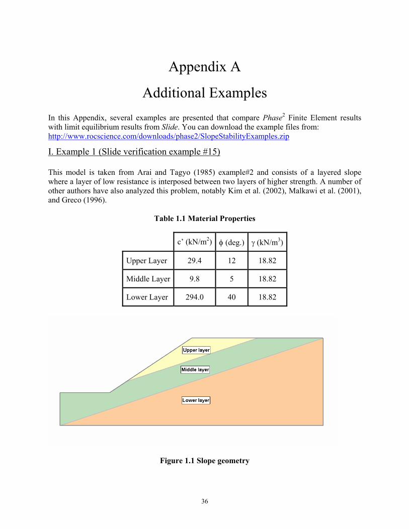
I. Example 1 (Slide verification example #15) This model is taken from Arai and Tagyo (1985) example#2 and consists of a layered slope where a layer of low resistance is interposed between two layers of higher strength. A number of other authors have also analyzed this problem, notably Kim et al. (2002), Malkawi et al. (2001), and Greco (1996).
Table 1.1 Material Properties
c’ (kN/m2) φ (deg.) γ (kN/m3)
Upper Layer 29.4 12 18.82
Middle Layer 9.8 5 18.82
Lower Layer 294.0 40 18.82
Figure 1.1 Slope geometry
36
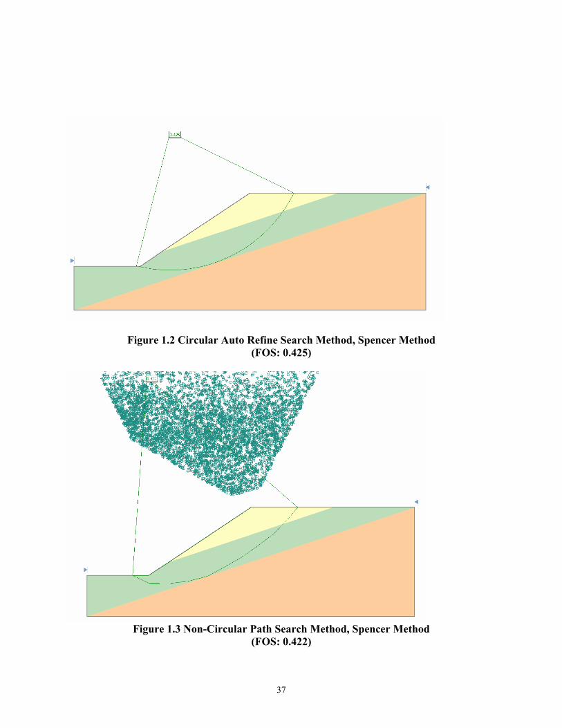
Figure 1.2 Circular Auto Refine Search Method, Spencer Method (FOS: 0.425)
Figure 1.3 Non-Circular Path Search Method, Spencer Method
(FOS: 0.422)
37
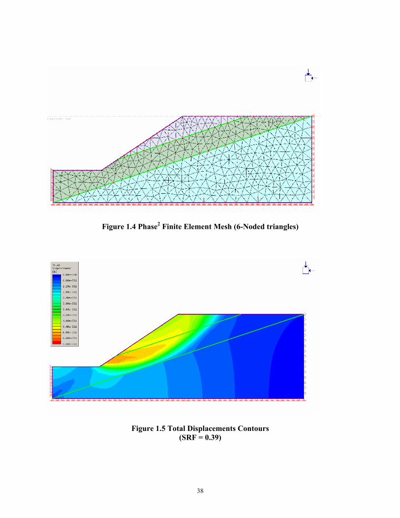
Figure 1.4 Phase2 Finite Element Mesh (6-Noded triangles)
Figure 1.5 Total Displacements Contours (SRF = 0.39)
38
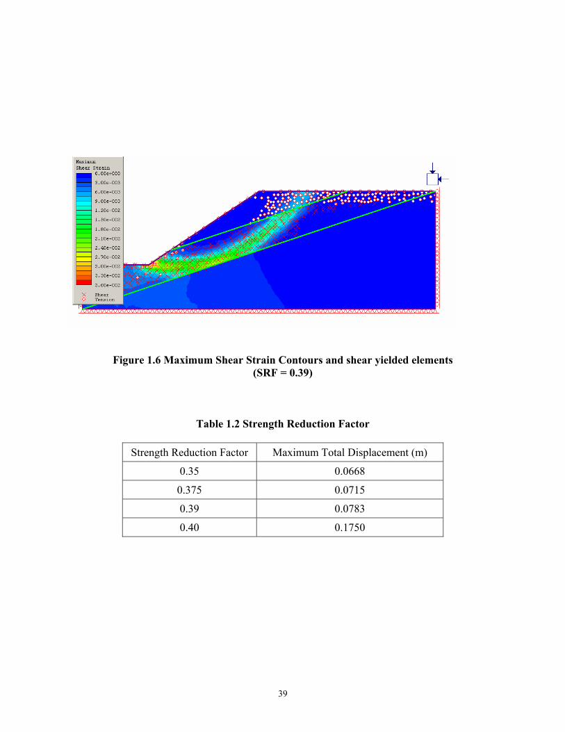
Figure 1.6 Maximum Shear Strain Contours and shear yielded elements (SRF = 0.39)
Table 1.2 Strength Reduction Factor
Strength Reduction Factor Maximum Total Displacement (m)
0.35 0.0668
0.375 0.0715
0.39 0.0783
0.40 0.1750
39
0.00
0.02
0.04
0.06
0.08
0.10
0.12
0.14
0.16
0.18
0.20
0.34 0.35 0.36 0.37 0.38 0.39 0.40 0.41
Strength Reduction Factor
Max
imum
Tot
al D
ispl
acem
ent (
m)
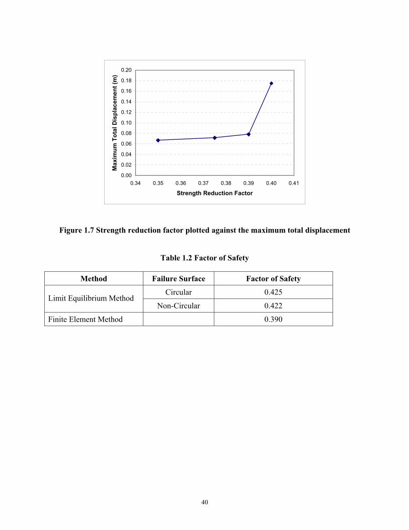
Figure 1.7 Strength reduction factor plotted against the maximum total displacement
Table 1.2 Factor of Safety
Method Failure Surface Factor of Safety
Circular 0.425 Limit Equilibrium Method
Non-Circular 0.422
Finite Element Method 0.390
40
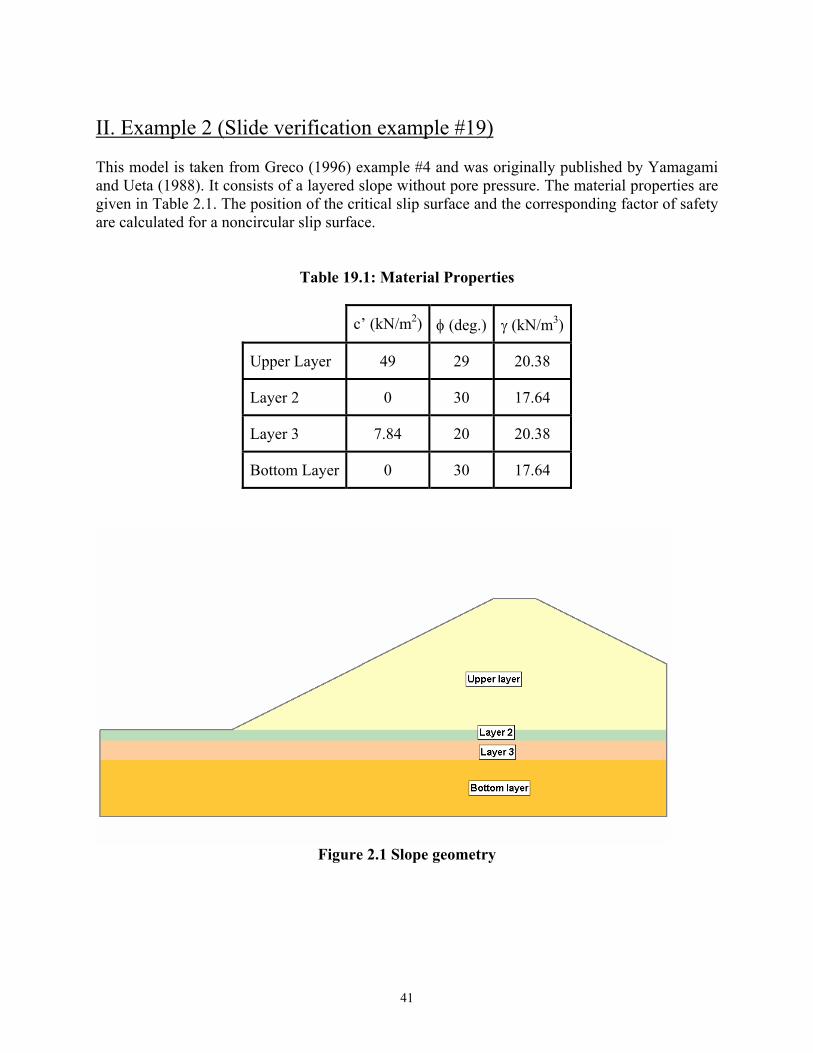
II. Example 2 (Slide verification example #19) This model is taken from Greco (1996) example #4 and was originally published by Yamagami and Ueta (1988). It consists of a layered slope without pore pressure. The material properties are given in Table 2.1. The position of the critical slip surface and the corresponding factor of safety are calculated for a noncircular slip surface.
Table 19.1: Material Properties
c’ (kN/m2) φ (deg.) γ (kN/m3)
Upper Layer 49 29 20.38
Layer 2 0 30 17.64
Layer 3 7.84 20 20.38
Bottom Layer 0 30 17.64
Figure 2.1 Slope geometry
41
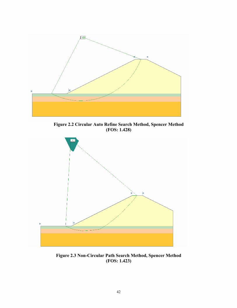
Figure 2.2 Circular Auto Refine Search Method, Spencer Method
(FOS: 1.428)
Figure 2.3 Non-Circular Path Search Method, Spencer Method (FOS: 1.423)
42
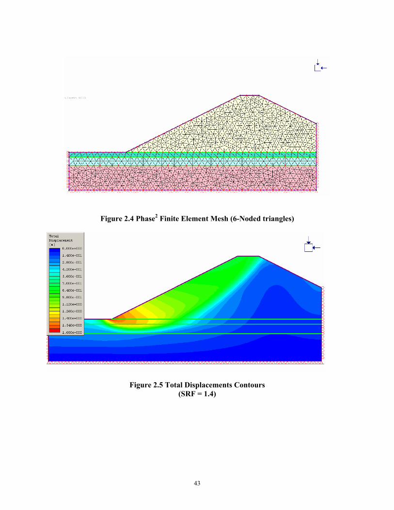
Figure 2.4 Phase2 Finite Element Mesh (6-Noded triangles)
Figure 2.5 Total Displacements Contours (SRF = 1.4)
43
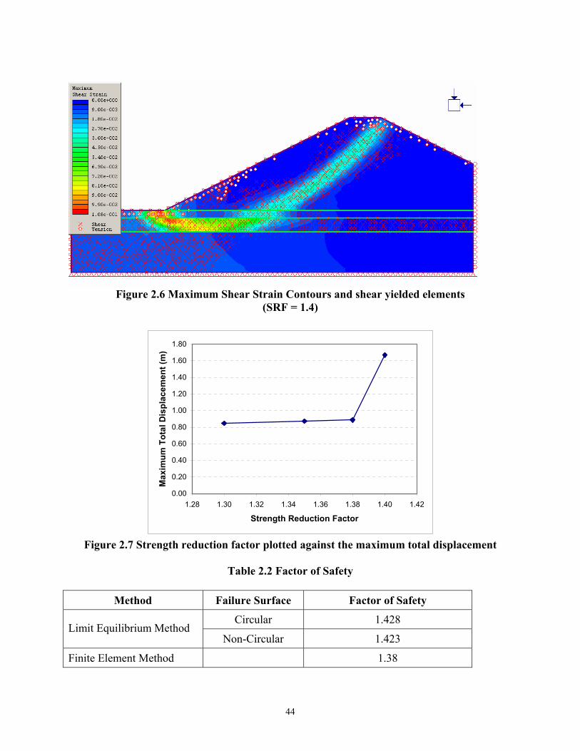
Figure 2.6 Maximum Shear Strain Contours and shear yielded elements
(SRF = 1.4)
0.00
0.20
0.40
0.60
0.80
1.00
1.20
1.40
1.60
1.80
1.28 1.30 1.32 1.34 1.36 1.38 1.40 1.42
Strength Reduction Factor
Max
imum
Tot
al D
ispl
acem
ent (
m)
Figure 2.7 Strength reduction factor plotted against the maximum total displacement
Table 2.2 Factor of Safety
Method Failure Surface Factor of Safety
Circular 1.428 Limit Equilibrium Method
Non-Circular 1.423
Finite Element Method 1.38
44
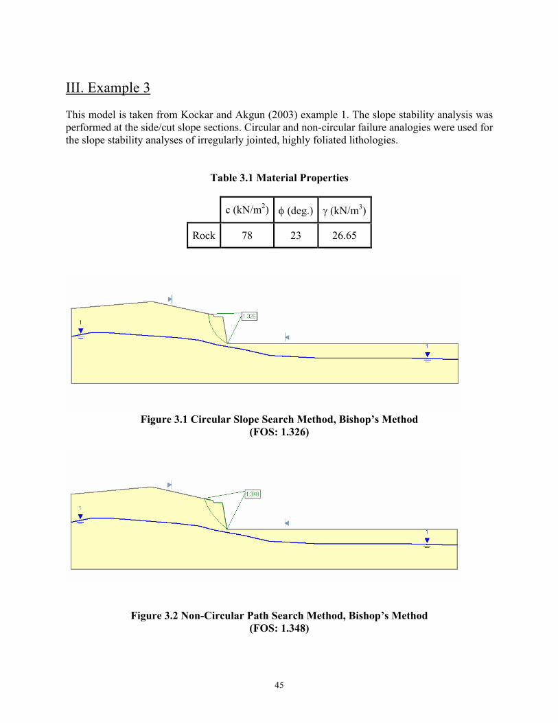
III. Example 3 This model is taken from Kockar and Akgun (2003) example 1. The slope stability analysis was performed at the side/cut slope sections. Circular and non-circular failure analogies were used for the slope stability analyses of irregularly jointed, highly foliated lithologies.
Table 3.1 Material Properties
c (kN/m2) φ (deg.) γ (kN/m3)
Rock 78 23 26.65
Figure 3.1 Circular Slope Search Method, Bishop’s Method
(FOS: 1.326)
Figure 3.2 Non-Circular Path Search Method, Bishop’s Method (FOS: 1.348)
45
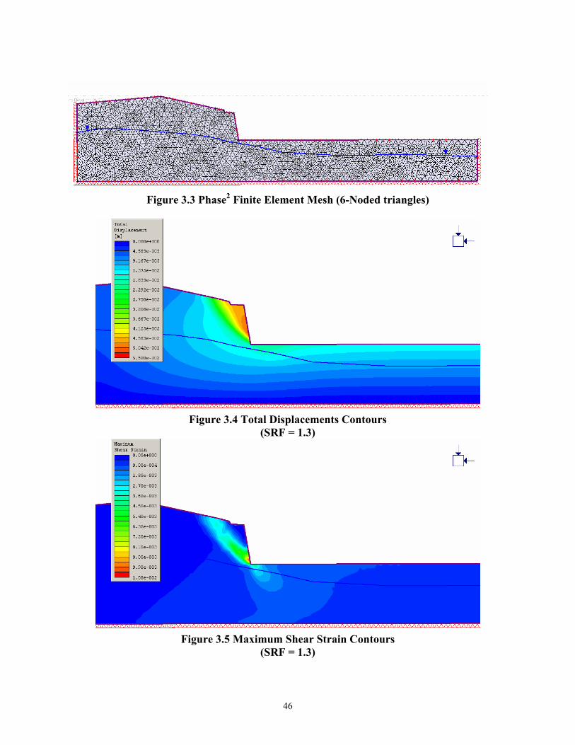
Figure 3.3 Phase2 Finite Element Mesh (6-Noded triangles)
Figure 3.4 Total Displacements Contours
(SRF = 1.3)
Figure 3.5 Maximum Shear Strain Contours
(SRF = 1.3)
46
0.00
0.01
0.02
0.03
0.04
0.05
0.06
0.07
0.08
0.09
0.10
1.15 1.20 1.25 1.30 1.35 1.40 1.45
Strength Reduction Factor
Max
imum
Tot
al D
ispl
acem
ent (
m)
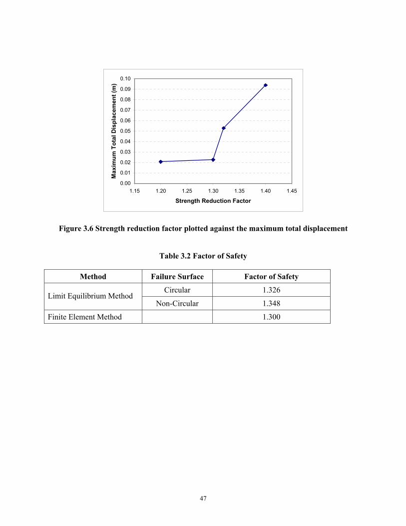
Figure 3.6 Strength reduction factor plotted against the maximum total displacement
Table 3.2 Factor of Safety
Method Failure Surface Factor of Safety
Circular 1.326 Limit Equilibrium Method
Non-Circular 1.348
Finite Element Method 1.300
47
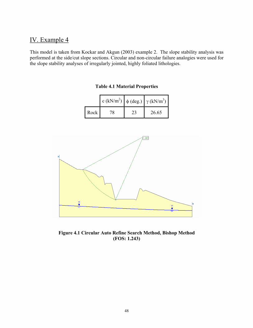
IV. Example 4 This model is taken from Kockar and Akgun (2003) example 2. The slope stability analysis was performed at the side/cut slope sections. Circular and non-circular failure analogies were used for the slope stability analyses of irregularly jointed, highly foliated lithologies.
Table 4.1 Material Properties
c (kN/m2) φ (deg.) γ (kN/m3)
Rock 78 23 26.65
Figure 4.1 Circular Auto Refine Search Method, Bishop Method
(FOS: 1.243)
48
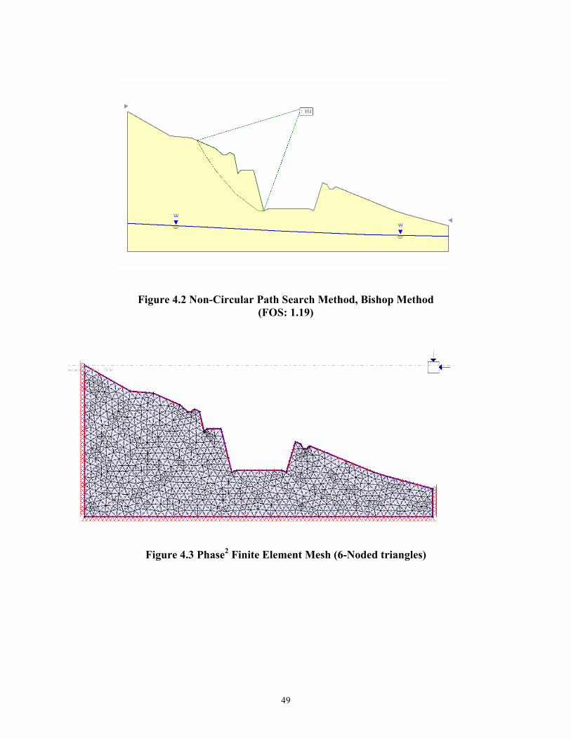
Figure 4.2 Non-Circular Path Search Method, Bishop Method (FOS: 1.19)
Figure 4.3 Phase2 Finite Element Mesh (6-Noded triangles)
49

Figure 4.4 Total Displacements Contours (SRF = 1.15)
Figure 4.5 Maximum Shear Strain Contours (SRF = 1.15)
50
0.00
0.01
0.02
0.03
0.04
0.05
0.06
0.07
0.95 1.00 1.05 1.10 1.15 1.20
Strength Reduction Factor
Max
imum
Tot
al D
ispl
acem
ent (
m)
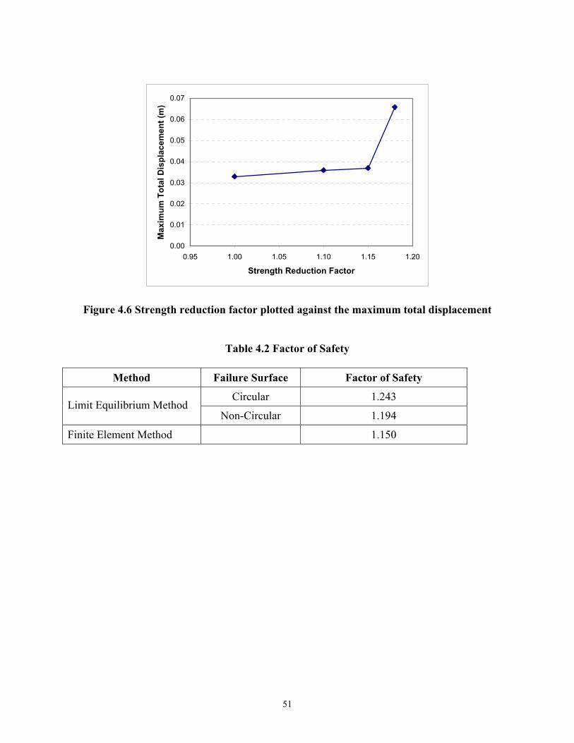
Figure 4.6 Strength reduction factor plotted against the maximum total displacement
Table 4.2 Factor of Safety
Method Failure Surface Factor of Safety
Circular 1.243 Limit Equilibrium Method
Non-Circular 1.194
Finite Element Method 1.150
51
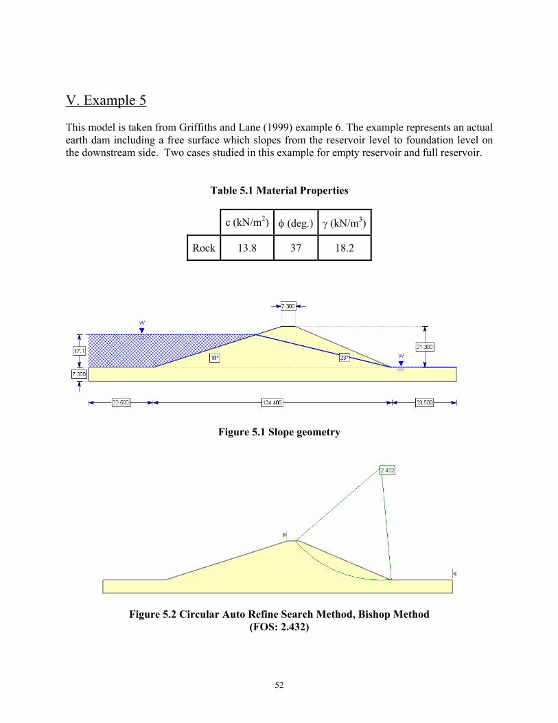
V. Example 5 This model is taken from Griffiths and Lane (1999) example 6. The example represents an actual earth dam including a free surface which slopes from the reservoir level to foundation level on the downstream side. Two cases studied in this example for empty reservoir and full reservoir.
Table 5.1 Material Properties
c (kN/m2) φ (deg.) γ (kN/m3)
Rock 13.8 37 18.2
Figure 5.1 Slope geometry
Figure 5.2 Circular Auto Refine Search Method, Bishop Method
(FOS: 2.432)
52
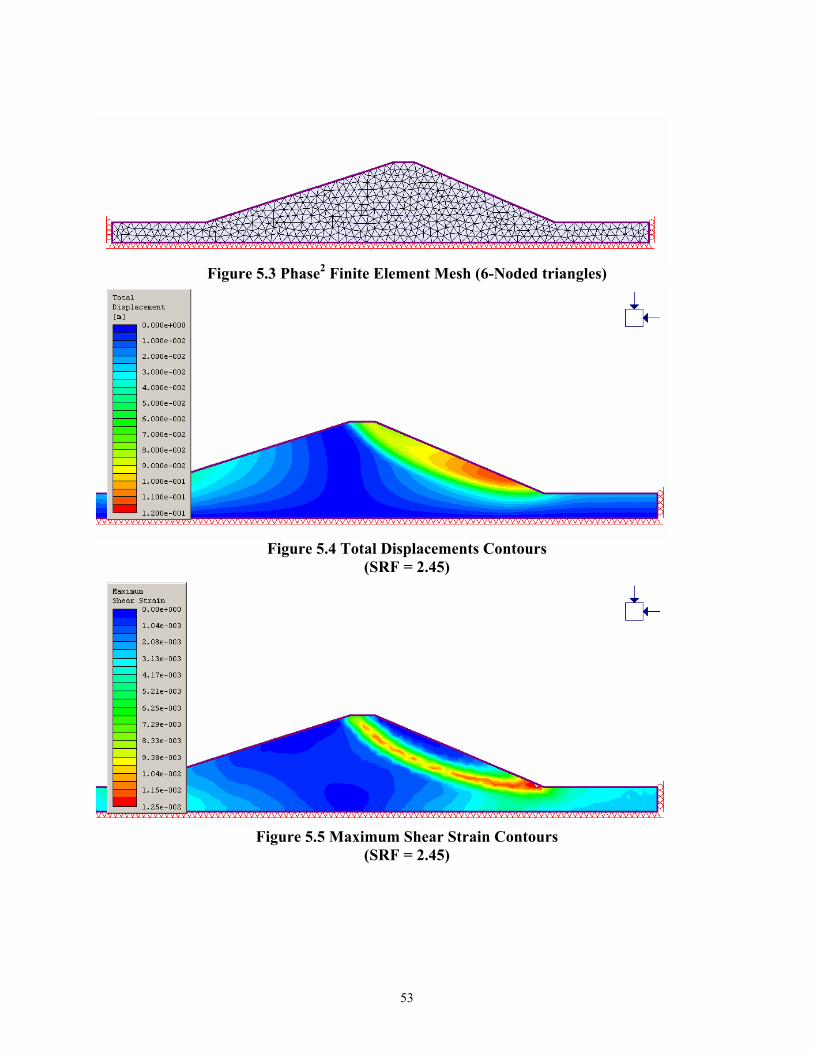
Figure 5.3 Phase2 Finite Element Mesh (6-Noded triangles)
Figure 5.4 Total Displacements Contours
(SRF = 2.45)
Figure 5.5 Maximum Shear Strain Contours
(SRF = 2.45)
53
0.00
0.02
0.04
0.06
0.08
0.10
0.12
0.14
0.16
0.18
2.25 2.30 2.35 2.40 2.45 2.50 2.55
Strength Reduction Factor
Max
imum
Tot
al D
ispl
acem
ent (
m)
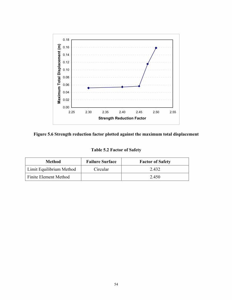
Figure 5.6 Strength reduction factor plotted against the maximum total displacement
Table 5.2 Factor of Safety
Method Failure Surface Factor of Safety
Limit Equilibrium Method Circular 2.432
Finite Element Method 2.450
54
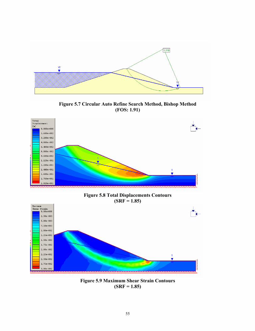
Figure 5.7 Circular Auto Refine Search Method, Bishop Method
(FOS: 1.91)
Figure 5.8 Total Displacements Contours
(SRF = 1.85)
Figure 5.9 Maximum Shear Strain Contours
(SRF = 1.85)
55
0.00
0.02
0.04
0.06
0.08
0.10
0.12
0.14
0.16
0.18
0.20
1.65 1.70 1.75 1.80 1.85 1.90 1.95
Strength Reduction Factor
Max
imum
Tot
al D
ispl
acem
ent (
m)
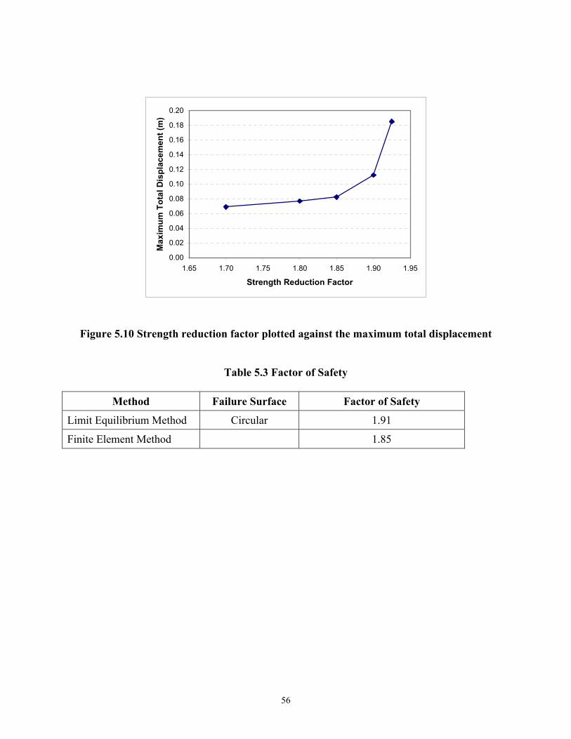
Figure 5.10 Strength reduction factor plotted against the maximum total displacement
Table 5.3 Factor of Safety
Method Failure Surface Factor of Safety
Limit Equilibrium Method Circular 1.91
Finite Element Method 1.85
56

57
Reference:
1. Arai, K., and Tagyo, K. (1985), “Determination of noncircular slip surface giving the minimum factor of safety in slope stability analysis.” Soils and Foundations. Vol.25, No.1, pp.43-51.
2. Malkawi, A.I.H.,Hassan, W.F., and Sarma, S.K. (2001), “Global search method for locating general slip surfaces using monte carlo techniques.” Journal of Geotechnical and Geoenvironmental Engineering. Vol.127, No.8, August, pp. 688-698.
3. Greco, V.R. (1996), “Efficient Monte Carlo technique for locating critical slip surface.” Journal of Geotechnical Engineering. Vol.122, No.7, July, pp. 517-525.
4. Kim, J., Salgado, R., Lee, J. (2002), “Stability analysis of complex soil slopes using limit analysis.” Journal of Geotechnical and Geoenvironmental Engineering. Vol.128, No.7, July, pp. 546-557.
5. Yamagami, T. and Ueta, Y. (1988), “Search noncircular slip surfaces by the Morgenstern-Price method.” Proc. 6th Int. Conf. Numerical Methods in Geomechanics, pp. 1335-1340.
6. M.K. Kockar, H. Akgun (2003), “Methodology for tunnel and portal support design in mixed limestone, schist and phyllite conditions: a case study in Turkey.” Int. J. Rock Mech. and Min Sci, Vol. 40, pp. 173–196.
7. Griffiths, D. V. and P. A. Lane (1999), "Slope Stability analysis by finite elements."
Geotechnique 49(3): 387-403.


![Finite Element Method [Slide]](https://img.dokumen.tips/doc/110x75/552e2fde4a79597f578b4893/finite-element-method-slide.jpg)


