ii

THE IMPACT OF FISHERIES’ SOCIO-ECONOMIC CONTRIBUTION ON POVERTY

REDUCTION IN NAMIBIA

BY

RAUNA MUKUMANGENI

12293438

A DISSERTATION SUBMITTED TO THE WESTMINSTER BUSINESS SCHOOL,

UNIVERSITY OF WESTMINSTER

FOR THE DEGREE OF

MA IN INTERNATIONAL ECONOMIC POLICY AND ANALYSIS

SUPERVISOR: DR. SHEIKH SELIM

AUGUST 2013

iii

ACKNOWLEDGEMENTS

My most sincere gratitude goes to the Almighty Father for none of this would be possible

without his guidance and protection.

Other thanks extend to & to whom I say remain blessed:

My supervisor Dr. Sheikh Selim for his absolute guidance, assistance, prompt responses

and valuable expert advice on economic growth.

Mr. S. I. Savva, I shall forever remain indebted to you.

Panduleni Kadhila-Amoomo, for being the brother I never had. No words I can say shall

ever fit to describe.

My beloved twosome, husband Luis Miguel and daughter Maria for the love and

understanding. A year away is too long.

My dear parents, you did not only give life to me, even at this mature age you still ensure

I persevere through it with ease. You are truly amazing.

The rest of my family especially the Kashaka family, for all that matters.

iv

ABSTRACT

Poverty is a problem facing Namibia. Economic growth might be the solution. Given the

importance of economic growth, it is necessary to analyse its determining factors. The fisheries

sector is one of the most important sectors in Namibia and so is its economic growth. The

purpose of the study is to investigate if economic growth, with particular emphasis of the

fisheries sector, has impacted on poverty reduction during the period of 1990-2011. A

neoclassical model framework as an important tool in economic growth analysis is used to

analyse the determinants of Namibia’s fisheries economic growth and its effect on the country’s

economic growth. Additionally, the country’s economic growth is analysed. Estimated factors

are initial GDP, gross fixed capital formation, fisheries growth, general government expenditure

and unemployment. Conditional convergence is found for the fisheries sector and for the

economy. Namibia’s economic growth in 1990-2011 is mostly explained by initial GDP and

unemployment. The study finds that the fisheries sector growth is negatively correlated with the

country’s economic growth. Results of the fisheries sector imply that there is a negative

relationship between initial GDP and the sector’s growth. Additionally, the sector’s

unemployment is positively correlated with its economic growth. Furthermore the results do not

find enough evidence to suggest that the fisheries sector impacts on poverty reduction. The

results are important for policy formulation; that employment is created and initial GDP is

lowered to ensure enhancement of Namibia’s economic growth. An enhanced economic growth

presents great potential for poverty reduction.

Key words: Namibia, economic growth, per capita GDP, neoclassical model, poverty, resource

rent, conditional convergence

v

ABBREVIATIONS

BON BANK OF NAMIBIA

GDP GROSS DOMESTIC PRODUCT

HDI HUMAN DEVELOPMENT INDEX

MFMR MINISTRY OF FISHERIES AND MARINE RESOURCES

MOF MINISTRY OF FINANCE

NPC NATIONAL PLANNING COMMISSION

NSA NATIONAL STATISTICS AGENCY

R&D RESEARCH AND DEVELOPMENT

TAC TOTAL ALLOWABLE CATCH

vi

Table of Contents

ACKNOWLEDGEMENTS ......................................................................................................................... iii

ABSTRACT ................................................................................................................................................. iv

ABBREVIATIONS ...................................................................................................................................... v

CHAPTER 1 ................................................................................................................................................. 1

INTRODUCTION ........................................................................................................................................ 1

CHAPTER 2 ................................................................................................................................................. 3

CONTEXT & RATIONALE ........................................................................................................................ 3

CHAPTER 3 ............................................................................................................................................... 11

LITERATURE REVIEW ........................................................................................................................... 11

CHAPTER 4 ............................................................................................................................................... 16

METHODOLOGY ..................................................................................................................................... 16

4.1 MODEL SPECIFICATION .............................................................................................................. 16

4.2 DATA ............................................................................................................................................... 17

4.3 METHODS ....................................................................................................................................... 22

CHAPTER 5 ............................................................................................................................................... 23

RESULTS AND ANALYSIS ..................................................................................................................... 23

CHAPTER 6 ............................................................................................................................................... 37

CONCLUSIONS AND RECOMMENDATIONS ..................................................................................... 37

REFERENCES ........................................................................................................................................... 43

APPENDICES ............................................................................................................................................ 51

1

CHAPTER 1

INTRODUCTION

1. INTRODUCTION

Poverty is a major problem facing Namibia. This study attempts to investigate the impact of

economic growth on poverty reduction in Namibia during 1990-2011. Similarly, the study

attempts to find empirical evidence on the determinants of economic growth in Namibia during

the period 1990-2011 using the neoclassical framework borrowed from the pioneer work of

Barro and Sala-i-Martin (2004). In view of the country being natural resources endowed, in

particular the fisheries sector as one of the main pillars of the Namibian economy, the sector’s

economic growth is investigated. The purpose of the study is to investigate if economic growth,

with particular emphasis of the fisheries sector, impacts on poverty reduction. In order to

effectively investigate the fisheries sector impact on poverty, the sector’s economic growth and

the country’s economic growth are investigated to find the relationship, if any, between the

respective economic growth and initial per capita GDP, gross fixed capital formation, fisheries

per capita GDP, general government expenditure and unemployment. The study tests three

hypotheses that correlate gross fixed capital formation, unemployment and initial per capita GDP

on economic growth.

The country is involved in efforts to increase economic growth and fight against poverty

(MOF, 2012). The issue of economic growth is important because it is a major factor in reducing

poverty. Barro and Sala-i-Martin (2004) underlined economic growth as possibly the one single

factor that influences income levels of individuals and advocate for the understanding of its

determining factors to solve economic related problems such as poverty.

Poverty is a phenomenon that faces many third world countries and Namibia is no exception.

According to NSA (2012), approximately 20% of the population in Namibia is poor and 14% is

severely poor and 19% of households are poor. Globally however, the total number of poor

people, as a result of economic growth, has reduced during the past three decades (World Bank,

2008).

2

Combating poverty is high on the agenda of many governments including the Namibian

government and the international community. Its eradication is the number one goal on the list

of Millennium Development Goals of the Millennium Declaration adopted by the United Nations

General Assembly on September 8, 2000 (Cypher and Dietz, 2009). The government has

outlined how it is to address poverty, job creation and economic growth in its Fourth National

Development Plan and Vision 2030 (NPC, 2012). Despite the government’s attempt to deal with

poverty, the problem persists (UNDP, 2007) and aggressive policy interventions are therefore

needed. Economic growth can be the engine to reduce poverty, and specifically the fisheries

sector can partake in this role. Mauritania and Vietnam are testimony that the fisheries sectors do

play a major role in economic growth and poverty reduction (Allison, 2011). Cypher and Dietz

(2009:31) defines economic growth as the rate of growth of income per person over time,

generally measured by Gross Domestic Product or Gross National Income.

Results imply that Namibia’s economic growth in 1990-2011 is determined by initial per capita

GDP and unemployment. Additionally, the fisheries sector’s economic growth is determined by

initial per capita GDP. A negative relationship is found between the fisheries sector and the

country’s economic growth. Furthermore, a negative relationship is found between the sector and

unemployment. The study does find enough evidence to suggest that the fisheries sector

contributes significantly to poverty reduction.

It is important to know that the fisheries sector referred to herein includes both the fishing and

fish processing sector. The words per capita GDP growth and economic growth are used

interchangeably.

The study is presented in 6 chapters. Chapter one introduces the topic to the reader; Chapter two

study background and rationale; Chapter three, the literature review; Chapter four, the study

methodology; Chapter five presents findings and analysis and finally Chapter five presents the

summary, conclusions and recommendations.

3

CHAPTER 2

CONTEXT & RATIONALE

2. DESCRIPTIVE BACKGROUND

In order to understand the poverty reduction potential of the fishery’s sector. It is necessary to

have context knowledge of the sector as well as of the Namibian economy.

2.1 NAMIBIA OVERVIEW

Namibia has a population of 2.3 million people and the second lowest world population density

after Mongolia (CIA, 2012). It is a resource based wealthy country, with abundant marine

fisheries (Arthur, et al., 2005), yet most of its citizens live in poverty (NPC, 2012). According to

the National Housing Income and Expenditure Survey (NHEIS) of 2009/10, the number of

households in Namibia is 436 795 (approximately 43.26% in urban and 56.7% in rural areas)

with an average of 4.7 people in each, an increase from 371 668 households in 2004 but with a

much higher average number 4.9 people. Furthermore, the country has a GDP of N$37,56 billion

and average GDP growth of 4% (figure 1 below) for the past 22 years, a poverty gap of 30%,

literacy 88% and per capita income approximated at N$34122 in 2011 (World Bank, 2013).

Figure 1: The economy and fisheries real GDP growth rates

Source: Compiled using World Bank data, 2013

4

Despite its high per capita income and economic growth, Namibia is a haven for poverty and

high unemployment levels.

Unemployment as a direct contributing factor to poverty is a big economic and social challenge

in Namibia (UNDP, 2007). Other challenges include inadequate economic growth and the

unequal distribution of income, all of which are interlinked (NPC, 2007). The unemployment

rate is 27% (NSA, 2012). Unemployment causes negative socio-economic ills such as crime,

poverty and others (Chamberlin and Yueh, 2006).

2.2 FISHERIES SECTOR

Namibian fishery’s resources are commercially exploited. According to MFMR (2009), the

Namibian fisheries sector is based on the Benguela current system which supports a rich stock of

marine resources. Namibia has a coastline of approximately 1,500km. Found in its waters are

plenty of high value fishery species such as hake, monkfish, orange roughy, rock lobster and

lower value but more abundant horse mackerel. On average 500 000 metric tonnes of fish are

landed every year.

The fisheries sector is among the top four sectors contributing to the economy (NPC, 2011). The

other sectors are agriculture, mining and tourism. The sector is the second highest foreign

currency earner to the economy after mining (MFMR, 2011). The sector’s economic output

contributes to employment, export earnings, GDP, revenue (taxation, licence fees, payment of

quota fees, foreign investment alliances) and notwithstanding the effect on upstream and

downstream industries as well as the spill-over effects especially for the regions in which fishing

takes place (MFMR, 2013); (Lange, 2003). Individually, fishing companies make socio

economic contributions such as building schools and clinics, giving bursaries to students, food

aid etc (MFMR, 2013). The sector plays a crucial role in the economy through its contribution to

economic growth, food security and livelihood.

According to the NHIES of 2009/10, about 49% of the population derive their income from

wages and salaries. This indicates how important a role employment plays in reducing poverty in

5

Namibia. The fisheries sector employs about 12825 people (MFMR, 2013) representing

approximately 1.3% of the total labour force and less than 1% of the total population.

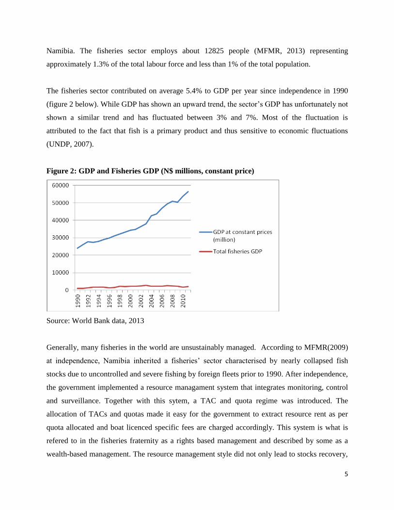
The fisheries sector contributed on average 5.4% to GDP per year since independence in 1990

(figure 2 below). While GDP has shown an upward trend, the sector’s GDP has unfortunately not

shown a similar trend and has fluctuated between 3% and 7%. Most of the fluctuation is

attributed to the fact that fish is a primary product and thus sensitive to economic fluctuations

(UNDP, 2007).

Figure 2: GDP and Fisheries GDP (N$ millions, constant price)

Source: World Bank data, 2013

Generally, many fisheries in the world are unsustainably managed. According to MFMR(2009)

at independence, Namibia inherited a fisheries’ sector characterised by nearly collapsed fish

stocks due to uncontrolled and severe fishing by foreign fleets prior to 1990. After independence,

the government implemented a resource managament system that integrates monitoring, control

and surveillance. Together with this sytem, a TAC and quota regime was introduced. The

allocation of TACs and quotas made it easy for the government to extract resource rent as per

quota allocated and boat licenced specific fees are charged accordingly. This system is what is

refered to in the fisheries fraternity as a rights based management and described by some as a

wealth-based management. The resource management style did not only lead to stocks recovery,

6

with the exception of pilchard but it also earned Namibia a place among the top countries with

sustainably managed marine resources (World Bank, 2013) next to renowned countries like

Iceland and Norway.

A good management of fisheries has positive meaning to poverty reduction because of the

national as well as local benefits through resource rent extraction, employment provision,

revenue to the state, trade associations as well as food security (FMSP, 2012). The idea of

sustainable natural resources is that capital is maintained intact, thus non declining over time

(Solow, 1986).

Namibia conquered the fight to sustainable marine resources; whether this translates to social

and economic benefits need to be investigated. If resource rent from the sector provides revenue

to the state and such revenues promote pro-poor growth, are reinvested in the economy i.e. in

services and infrastructure for the poor, the sector can contribute to poverty reduction (Allison,

2011). Namibia is among the few fishing nations that succeeded in capturing considerable

resource rent from its marine resources. Iceland and Norway are example of countries whose

natural resources such as fish are significant determinants of their economic growth (Gerlagh and

Papyrakis, 2007).

To empower citizens in fisheries, a policy of Namibianisation resulted in increased participation

by natives because of its selective support for the granting of fishing rights to Namibian-owned

companies and this may have potential positive benefits for Namibians (NPC, 2012).

2.3 POVERTY

Namibia is a former German colony, a developing nation in Sub-Sahara Africa and is among the

54 upper middle income countries of the world (World Bank, 2013). As a former colony, the

country has not completely severed ties with its former regime as many historical traits from the

past, economic or social, remain to haunt it to this day. Among those are income inequalities and

poverty (World Bank, 2013).

7

According to NHIES (NSA, 2012) 20% of households in Namibia are poor and 10% severely

poor. The number is said to have reduced from 24% and 14% in 2003/2004 respectively. The

poverty line in Namibia is N$2041 per month. Poverty is high in rural areas (27%) compared to

urban areas (9%) and mainly affects women (22% of female headed households), people with

low education attainment and farmers.

Many developing nations struggle with the challenge of reducing poverty (UNDP, 2007). Where

income inequality is prevalent, the problem of poverty is highly likely also. Income inequality

aggravates poverty (Seligson and Passe-Smith (2008). Income inequality refers to the gap

between the rich and the poor (Beckford, 2011), the unequal distribution of household or

individual income across the various participants in an economy (NSA, 2012). With a GINI

coefficient of 0.597 (NSA, 2012), Namibia is rated to be among nations with the highest unequal

distribution of income in the world and among nations with the highest poverty levels in Sub

Sahara Africa (World Bank, 2013). Income inequality is therefore another major social problem

facing Namibia and a main cause of poverty in Namibia.

According to Acemoglu, Johnson and Robinson (2001), inequalities in some countries, for

example Namibia, were predestined because of historical ties to Europeans who set up

institutions in their colonies for easy resource transfers. To support this fact, Namibia continues

to be a primary fishery sector exporter (MFMR, 2011). Approximately 90% of the fish and fish

products are exported to European markets most with no or minimal value added (MFMR,

2009).

Namibia’s main source of poverty originated from the colonialism era before independence in

1990, from which income disparity between different ethnic factions (based on discrimination

policies that limited the majority access to social and economic resources) existed (NPC, 2007).

A classic example is that due to historical ties, the German headed households who only make up

a part of the 6% of white minority in Namibia continue to command power over the Namibian

economy. According to NSA (2012) German households make up a mere 0.4% of the 436 795

1 Approximately US$28. 1US$=N$7.26 annual average exchange rate of 2011 (source: World Bank, 2013)

8

total households in the country. Relative to all the households, they have the highest asset

ownership (be it land, housing, transport etc), highest per capita income, highest cash

expenditure, spend the most on recreation; enjoy the best education and health. They simply have

the best of everything in Namibia. Without implying that historical institutions cannot be

changed Acemoglu, Johnson and Robinson (2001), argues that their influence still remained in

the colonies. Economic growth and structural change can change poverty and for this to happen,

breaking ties with past structures is imminent (Cypher and Dietz, 2009: 19).

Regardless of colonial ties, the Namibian government is committed to economic growth

stimulation with the purpose of reducing income inequalities and poverty (NPC, 2007).

Intentions of the government for a pro-poor economic growth have been echoed in the budget

speeches increasingly over time. During the 2012/13 budget speech the government announced

its recent effort, the Targeted Intervention Program for Employment and Economic Growth

(TIPEEG) and more funds continue to be allocated to health and education (MOF, 2012).

Investing in human capital is argued to be an engine for economic growth and equity (Seligson

and Passe-Smith, 2008). Classical and neo classical economists like Adam Smith; Solow,

Domar and others identified determinants of economic growth as physical capital accumulation,

labour or natural resources, technology, savings and investment (Cypher and Dietz, 2009). They

emphasized that countries intending to grow their economies and improve their social status

should ensure that these determinants are clearly understood and in order.

High inequality levels have dramatic effects on economic growth of a nation and t hus

changes in poverty and inequality are key indicators of economic progress and social enclosure

(NSA, 2012). However caution should be exercised as one cannot view the growing GDP per

capita alone as economic growth (NSA, 2012), as economic growth depends on much more,

hence lately the HDI is additionally used (UNDP, 2013). Namibia has an HDI of 0.625, which

generally implies that the economy is probably 62.5% enabling or conducive for individuals to

grow and better their living standards (UNDP, 2013).

9

2.4 RATIONALE

In view of the contribution of the fisheries sector to the economy and the fact that the sector is

among the top contributing to GDP, it is expected that its economic growth impacts positively on

poverty reduction.

Poverty in Namibia is a never ending, disturbing condition. Time and time again stories of poor

people are narrated in the media and one also does not need to look far to find a poverty victim.

It is established from the review of different literature that much has been done to combat this

evil but efforts do not appear to deliver substantial results. It is very important to understand how

Namibia’s fishery sector contributes to the country’s poverty reduction through its activities

contributions.

A study of this kind is important for various reasons. From a policy perspective its findings will

contribute to shaping policy in that they will be evidence based policy suggestions. The study

will present policy makers with an additional source of information for evaluation of the fisheries

sector that could help improve fisheries performance in the context of overall national economic

goals. The study will also contribute to the knowledge and literature available on the fisheries’

sector economic growth that basically serves to facilitate an understating of the reader’s

knowledge of the sector. Additionally, the study findings will give the reader information on the

role the fisheries sector plays on poverty reduction.

The researcher found interest in the study with the aim of acquiring deeper knowledge of the

sector and to seek answers on whether the abundant fisheries resource contributes to poverty

reduction. Considering the fact that Namibia is a resource abundant country, the issue of poverty

in Namibia raises concern. Poverty deprives people of opportunities such as education. It affects

the poor’s chances to efficiently contribute to the economy and thus halts economic growth

hence increases opportunity cost of poor people who could otherwise be productive members of

society. This does not only affect the poor individuals but goes on to affect the economy in a

broader context through forgone potential tax revenues. The researcher found it disturbingly

challenging to comprehend how Namibia, a low densely populated country is inhabited by

10

destitute people that languish in immense poverty when endowed with resources like fisheries

that are applauded for their worth around the globe. Against this the researcher was motivated to

undertake the study. Last but not least, the study will provide information to future researchers

who may wish to study the relationship between economic growth and fisheries as well as its

economic contributions thereof.

Expectations are on the fisheries sector to create jobs, generate revenue and contribute to poverty

reduction. It is not clear how the sector reduces the high level of poverty in Namibia despite its

economic contributions to the economy. Against this background the study was deemed

necessary.

11

CHAPTER 3

LITERATURE REVIEW

The literature review was conducted mainly using online sources including journals, articles and

other relevant literature. A few books were also borrowed from the university library. The

review attempted to investigate what has been written by other researchers on capital

accumulation, government expenditure, fisheries growth, initial GDP and economic growth and

how the latter with emphasis on the fisheries sector economic growth, affects poverty. Although,

sufficient literature relating to the current study was found, limited empirical literature on

economic growth, the fisheries sector and poverty reduction on Namibia was available.

The neoclassical theory is the general first point for theoretical and empirical literature on

economic growth. Despite criticism for failure to explain technological progress (Levine, 1998)

the theory states that a national economic growth depends on physical and human capital

accumulation, savings and technology (exogenously determined in the long run), which are

determined by country specific factors. Theory predicts a negative partial correlation between

growth and the initial level of income, also referred to as conditional convergence (Barro and

Sala-i-Martin (2004: 519) the coefficient of log of initial income is the rate of responsiveness of

the growth rate. The conditional convergence is a significant determinant of economic growth. It

gives an idea about how far an economy is in terms of its long run/steady state position (Barro

2004: 17) and according to theory, the further away it is, the faster the economy will grow. The

empirical study of Gerlagh and Papyrakis (2007) and many others reiterate the importance of

conditional convergence as an important determinant of economic growth.

An investigation of the variables that impact on economic growth is very important when dealing

with the economy and trying to understand its economic growth prospective as well as its

potential to reduce poverty. One notable empirical study on economic growth is by Barro and

Sala-i-Martin (2004) who investigated economic growth determinants of 87 countries using cross

section data and found that economic growth positively depends on human capital (educational

attainment & health), maintenance of the rule of law, investment and negatively on government

consumption and fertility rates. They found conditional convergence when other variables that

12

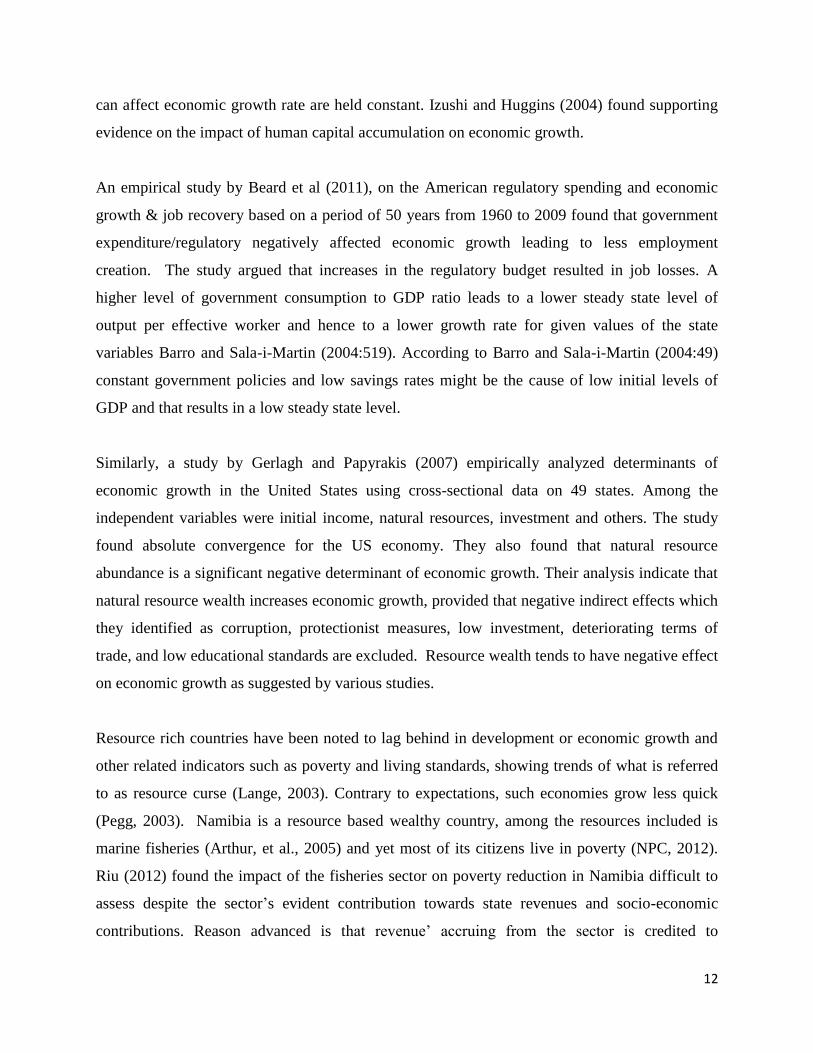
can affect economic growth rate are held constant. Izushi and Huggins (2004) found supporting

evidence on the impact of human capital accumulation on economic growth.

An empirical study by Beard et al (2011), on the American regulatory spending and economic

growth & job recovery based on a period of 50 years from 1960 to 2009 found that government

expenditure/regulatory negatively affected economic growth leading to less employment

creation. The study argued that increases in the regulatory budget resulted in job losses. A

higher level of government consumption to GDP ratio leads to a lower steady state level of

output per effective worker and hence to a lower growth rate for given values of the state

variables Barro and Sala-i-Martin (2004:519). According to Barro and Sala-i-Martin (2004:49)

constant government policies and low savings rates might be the cause of low initial levels of

GDP and that results in a low steady state level.

Similarly, a study by Gerlagh and Papyrakis (2007) empirically analyzed determinants of

economic growth in the United States using cross-sectional data on 49 states. Among the

independent variables were initial income, natural resources, investment and others. The study

found absolute convergence for the US economy. They also found that natural resource

abundance is a significant negative determinant of economic growth. Their analysis indicate that

natural resource wealth increases economic growth, provided that negative indirect effects which

they identified as corruption, protectionist measures, low investment, deteriorating terms of

trade, and low educational standards are excluded. Resource wealth tends to have negative effect

on economic growth as suggested by various studies.

Resource rich countries have been noted to lag behind in development or economic growth and

other related indicators such as poverty and living standards, showing trends of what is referred

to as resource curse (Lange, 2003). Contrary to expectations, such economies grow less quick

(Pegg, 2003). Namibia is a resource based wealthy country, among the resources included is

marine fisheries (Arthur, et al., 2005) and yet most of its citizens live in poverty (NPC, 2012).

Riu (2012) found the impact of the fisheries sector on poverty reduction in Namibia difficult to

assess despite the sector’s evident contribution towards state revenues and socio-economic

contributions. Reason advanced is that revenue’ accruing from the sector is credited to

13

government coffers for countrywide appropriation purposes and programs. In agreement Allison,

Béné and Macfadyen (2007) suggest that it is easier to study the relationship between poverty

reduction and small scale fisheries because of its highly significant direct linkages as opposed to

commercial fisheries.

Allison (2011) found evidence that the fisheries sector influences economic growth through

increased cash but found little direct quantitative evidence of the magnitude of the multiplier

effect. Case studies on 8 different countries done by DFID (2005) found that wealth created by

fisheries was appropriated in a manner that contributed to economic growth and poverty

reduction. Lange (2003) studied wealth (natural, human and social capital) data for Namibia for

1980-2000 and found that Namibia did not invest sufficiently in line with population growth and

was thus liquidating its capital which caused low economic growth. Solow, (1986) argues for the

Hartwick’s rule, that suggests reinvesting rent from natural resources in reproductive capital is a

way to maintain capital stock but cautioned against the un-established effect from endogenous

variables such as population growth and technology.

Allison, Béné and Macfadyen (2007) argues for a right based management system against the

background that inefficiency in the fishery sector resulted in misuse of assets and suggest that

there is economic growth opportunity from fisheries if the economic rents are reasonably

captured and reinvested in public goods. Additionally, he argues that accountability of such

rents were a determinant of the degree of economic growth from the fisheries sector.

Furthermore, he notes that too much concentration on improving access rights to fisheries by the

poor limited wealth generation potential of fisheries. In his study on countries that include

Philippines and Solomon Island he analyzed a 30 year time series of exports and found that there

was a negative relationship between population growth, high domestic consumption, persistent

poverty and the availability of fish in the local market suggesting that trade of natural resources

i.e. fish contributed negatively to economic growth. In disagreement to keep fisheries access

limited, but in agreement to the relationship between economic growth and poverty, Chong

(1993) argues that limited entry to fisheries especially in developing countries with abject

poverty was not pleasant because it tends to keep small scale fishermen poor. Of a different

finding are Eita and Jordaan (2007) who used time series econometric data of Namibia for 1970-

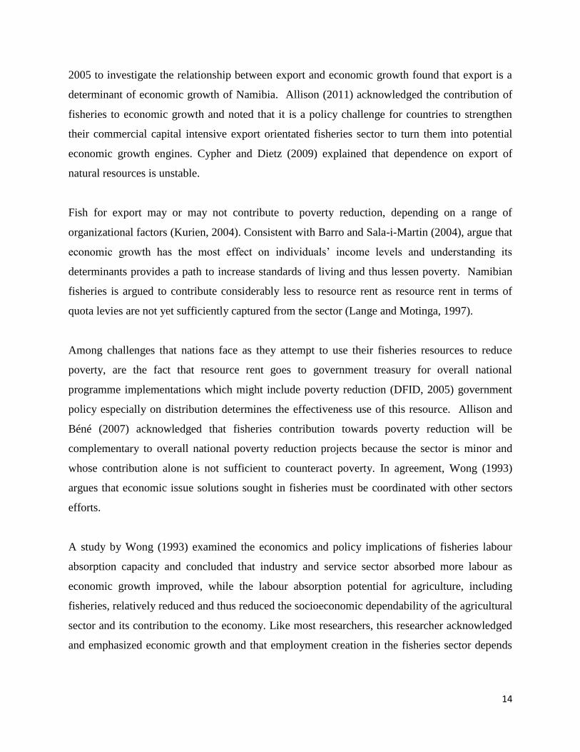
14

2005 to investigate the relationship between export and economic growth found that export is a

determinant of economic growth of Namibia. Allison (2011) acknowledged the contribution of

fisheries to economic growth and noted that it is a policy challenge for countries to strengthen

their commercial capital intensive export orientated fisheries sector to turn them into potential

economic growth engines. Cypher and Dietz (2009) explained that dependence on export of

natural resources is unstable.

Fish for export may or may not contribute to poverty reduction, depending on a range of

organizational factors (Kurien, 2004). Consistent with Barro and Sala-i-Martin (2004), argue that

economic growth has the most effect on individuals’ income levels and understanding its

determinants provides a path to increase standards of living and thus lessen poverty. Namibian

fisheries is argued to contribute considerably less to resource rent as resource rent in terms of

quota levies are not yet sufficiently captured from the sector (Lange and Motinga, 1997).

Among challenges that nations face as they attempt to use their fisheries resources to reduce

poverty, are the fact that resource rent goes to government treasury for overall national

programme implementations which might include poverty reduction (DFID, 2005) government

policy especially on distribution determines the effectiveness use of this resource. Allison and

Béné (2007) acknowledged that fisheries contribution towards poverty reduction will be

complementary to overall national poverty reduction projects because the sector is minor and

whose contribution alone is not sufficient to counteract poverty. In agreement, Wong (1993)

argues that economic issue solutions sought in fisheries must be coordinated with other sectors

efforts.

A study by Wong (1993) examined the economics and policy implications of fisheries labour

absorption capacity and concluded that industry and service sector absorbed more labour as

economic growth improved, while the labour absorption potential for agriculture, including

fisheries, relatively reduced and thus reduced the socioeconomic dependability of the agricultural

sector and its contribution to the economy. Like most researchers, this researcher acknowledged

and emphasized economic growth and that employment creation in the fisheries sector depends

15

on it. Similarly, Allison (2011) argues that substitution of labour by technology reduces

employment in the fisheries sector.

Limited researches into the links and underlying contributory factors between fisheries and

poverty, and development of strategies to maximize the welfares derived from fisheries to reduce

the poverty (FMSP, 2012), has been identified as a gap that this research somehow intends to

contribute to. Economic growth is presented by literature to be of crucial importance in

employment creation and poverty reduction.

16

CHAPTER 4

METHODOLOGY

4.1 MODEL SPECIFICATION

To explain the variations in economic growth of Namibian during 1990-2011, the fisheries sector

and the economy’s economic growth are estimated using per capita growth regressions. The

purpose is to determine if the fishery’s sector impacts on poverty reduction through economic

growth. The fisheries sector’s economic growth as well as that of the country is investigated

through the respective relationship between the two and the initial per capita GDP growth, initial

per capita fisheries GDP growth, fisheries gross capital formation, gross capital formation,

general government expenditure: income, expenditure & savings growth rate, unemployment

growth rate. The regression analyses estimates two main models varied in explanatory variables

but at both times have the relevant either per capita GDP growth or per capita fisheries GDP

growth rate as the dependent variable. For each model, two equations are estimated.

The empirical framework, a neoclassical growth model as discussed by Barro and Sala-i-Martin

(2004), is altered into two main growth functions to suit the study. The per capita GDP growth

model and the fisheries per capita GDP growth model are used as per the equations presented in

1, 2, 3 & 4 below. The model assumes conditional convergence.

4.1.1 The basic per capita GDP growth model

The second model equation excludes the variable of fisheries per capita GDP.

17

Where, is growth rate; is per capita Gross Domestic Product growth rate; is the

constant; are partial regression coefficients; 2 is the conditional

convergence / initial real GDP growth rate; is is growth rate of gross fixed

capital formation; is growth rate of government expenditure; is the growth rate

of fisheries per capita Gross Domestic Product; is unemployment growth rate; is

dummies for the different time periods and u represents all other variables that affect but

are not explicitly included in the regression.

4.1.2 The basic per capita fisheries GDP growth model

The basic model equation is:

The second model equation excludes the gross formation variable of fisheries GDP growth rate.

Where, is growth rate; is Gross Domestic Product growth rate; is the constant;

are partial regression coefficients; is the initial real fisheries GDP

growth rate; is fisheries Gross Domestic Product growth rate; is government

expenditure growth rate; is unemployment growth rate; dummies for different time

periods and the u is the error term that represents all factors that affect but are not

explicitly included in the study.

4.2 DATA

Using time series and cross section data the relationships between the initial GDP, gross fixed

capital formation, government expenditure, unemployment and the respective fisheries economic

2 Lag(lnCGDP) equals log CGDP. Most studies use log instead of lag of log. The two mean the same thing.

18

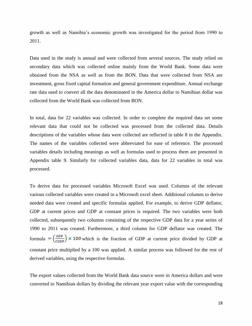
growth as well as Namibia’s economic growth was investigated for the period from 1990 to

2011.

Data used in the study is annual and were collected from several sources. The study relied on

secondary data which was collected online mainly from the World Bank. Some data were

obtained from the NSA as well as from the BON. Data that were collected from NSA are

investment, gross fixed capital formation and general government expenditure. Annual exchange

rate data used to convert all the data denominated in the America dollar to Namibian dollar was

collected from the World Bank was collected from BON.

In total, data for 22 variables was collected. In order to complete the required data set some

relevant data that could not be collected was processed from the collected data. Details

descriptions of the variables whose data were collected are reflected in table 8 in the Appendix.

The names of the variables collected were abbreviated for ease of reference. The processed

variables details including meanings as well as formulas used to process them are presented in

Appendix table 9. Similarly for collected variables data, data for 22 variables in total was

processed.

To derive data for processed variables Microsoft Excel was used. Columns of the relevant

various collected variables were created in a Microsoft excel sheet. Additional columns to derive

needed data were created and specific formulas applied. For example, to derive GDP deflator,

GDP at current prices and GDP at constant prices is required. The two variables were both

collected, subsequently two columns consisting of the respective GDP data for a year series of

1990 to 2011 was created. Furthermore, a third column for GDP deflator was created. The

formula which is the fraction of GDP at current price divided by GDP at

constant price multiplied by a 100 was applied. A similar process was followed for the rest of

derived variables, using the respective formulas.

The export values collected from the World Bank data source were in America dollars and were

converted to Namibian dollars by dividing the relevant year export value with the corresponding

19

annual average exchange rate. The exchange rate ranged between N$2.54 in 1990 and N$10.54

in 2002 and averaged N$5.94.

Some variables had missing data which were replaced. The electricity variable missing values for

the years 2011 and 1990 were replaced with the values of 2010 and 1991 respectively. Internet

users (per 100 people) and mobile cellular subscriptions had missing values from 1990 to 1994.

There was no use of mobiles and internet in Namibia during that time hence no data recorded.

Not all the variables were used in the final models because of several reasons which include but

are not limited to collinearity. Correlation analyses led to the exclusion of some variables such as

electricity, telecommunications, mortality rate (neonatal), improved sanitation and export index

from the final models. Some variables showed strong correlation among them and thus could not

be used together. Such strong correlation can mean that the excluded variables’ influence can be

explained by the remaining variables. For example telecommunication and electricity can be

explained by gross rate of capital formation which includes all general investment made and thus

having both (electricity and telecommunication) in the model would make no sense. The two

final models include only variables that are not correlated and thus do not violate the

assumptions of multiple regression.

According to Berenson et al (2011), the standard multiple regression assumptions are that:

The independent variables are not correlated

The residuals follow the normal distribution with mean 0.

The residuals are independent

The variance of the residuals is constant across observations (homoscedasticity).

The independent variables and the dependent variable have a linear relationship.

Correlation analyses were done to ensure that there is no multicollinearity between the

independent variables. Correlation matrices are presented in tables 6 & 7 in the Appendix.

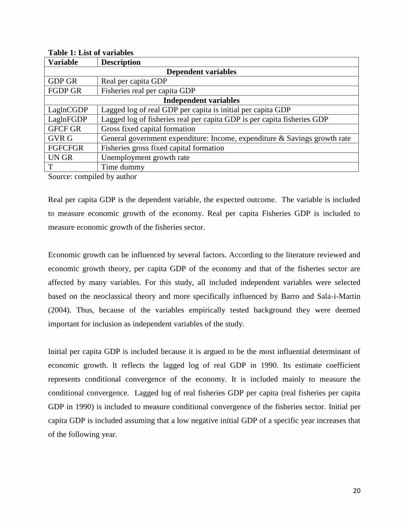
Table 1 below reflects a list of variables that were deemed important determinants of economic

growth in Namibia during 1990-2011.

20

Table 1: List of variables

Variable Description

Dependent variables

GDP GR Real per capita GDP

FGDP GR Fisheries real per capita GDP

Independent variables

LaglnCGDP Lagged log of real GDP per capita is initial per capita GDP

LaglnFGDP Lagged log of fisheries real per capita GDP is per capita fisheries GDP

GFCF GR Gross fixed capital formation

GVR G General government expenditure: Income, expenditure & Savings growth rate

FGFCFGR Fisheries gross fixed capital formation

UN GR Unemployment growth rate

T Time dummy

Source: compiled by author

Real per capita GDP is the dependent variable, the expected outcome. The variable is included

to measure economic growth of the economy. Real per capita Fisheries GDP is included to

measure economic growth of the fisheries sector.

Economic growth can be influenced by several factors. According to the literature reviewed and

economic growth theory, per capita GDP of the economy and that of the fisheries sector are

affected by many variables. For this study, all included independent variables were selected

based on the neoclassical theory and more specifically influenced by Barro and Sala-i-Martin

(2004). Thus, because of the variables empirically tested background they were deemed

important for inclusion as independent variables of the study.

Initial per capita GDP is included because it is argued to be the most influential determinant of

economic growth. It reflects the lagged log of real GDP in 1990. Its estimate coefficient

represents conditional convergence of the economy. It is included mainly to measure the

conditional convergence. Lagged log of real fisheries GDP per capita (real fisheries per capita

GDP in 1990) is included to measure conditional convergence of the fisheries sector. Initial per

capita GDP is included assuming that a low negative initial GDP of a specific year increases that

of the following year.

21

Gross fixed capital formation is included to control for the total value of physical capital. This

can be investment in human capital, R&D, acquiring more assets etc. It has been proven that

investment in human capital, for example, increases their productivity and this can lead to

economic growth. It is an important determinant of conditional convergence and economic

growth. Fisheries gross capital formation controls for the specific fisheries investments

influence on economic growth during 1990-2011. Investments in the fishery sector especially in

vessels tend to result in over capacity of the sector leading to loss of efficiency and might

negatively affect economic growth.

General government expenditure measures the influence of government income, expenditure and

savings on economic growth. The positive effect of government spending on economic growth

will depend on what, and perhaps at which sector the expenditure is directed. If for example the

government spends on health and education, that will be considered positive because education

and health play very important roles in the development of an economy and leads to better

opportunities for people to better their living standards. If government expenditure results in

crowding out or leads to important project delays, then investment may not be desired. The

estimate is expected to have a negative sign (according to the Ricardian view3). Time dummy is

included to control for the different time periods.

Unemployment is included because it is high in Namibia and it has direct influence on poverty

which the study intends to analyze. Employment is a mean to receiving an income. Many people

in Namibia derive their income from wages (NSA, 2012). Employment has a positive effect on

economic growth (Beard et al, 2011). According to Chamberlin & Yueh (2006) unemployment

has two main costs that are social and economic with the latter being largely efficiency and

budgetary. It erodes efficiency because of human resource underutilization. Socially, it leads to

poverty, low health etc. The coefficient is expected to have a negative sign.

3 David Ricardo, Ricardian view argues against government role. Generally this sign is expected to be positive if

Keynesian view is followed (C+I+G+(X-M)). In this study, the expected sign is negative since the model used is

neoclassical.

22

Economic growth is the desired outcome; therefore the selected influential variables will be

investigated to determine their effect on economic growth.

4.3 METHODS

All data collected were entered in Microsoft excel spread sheet. Thereafter the data was uploaded

to Statistical Package for Social Sciences (SPSS) were all analyses were done. The data was

analysed using linear multiple regressions, bivariate regressions and significances were tested

using t-tests and F-tests.

Using data and regressions the four equations specified under “model specification” were

estimated. The growth relationship was applied to give an indication of how each identified

explanatory variables explain variations in per capita GDP growth and the fisheries per capita

GDP growth. Each independent variable’s effect on the relevant dependent variable was

established while controlling for the effects of other independent variables.

23

CHAPTER 5

RESULTS AND ANALYSIS

Presented below and accordingly are the results of the analyses from the four regressed

equations.

Descriptive statistics give an overview of the central tendencies of the variables such as how

much the economy grew on average per year or what the minimum or maximum of a specific

variable was, during the period under review.

5.1 Basic per capita GDP Growth model (equation 1)

Table 3 presents regression results for the basic per capita GDP growth regression. The estimated

equation can be written as:

Tables 11-13 in the Appendix present the descriptive statistics, ANOVA and model summary

outputs respectively. Descriptive statistics results show that initial GDP had the highest growth

of 10.5% on average per year followed by unemployment at -0.14%. Interestingly, growth of

GDP, fisheries sector GDP growth and gross fixed capital formation averaged 0.04% per year

during 1990-2011. The results also show that the least the economy grew is by -1% during 2009

while maximum is 12.3% during 2004. The lowest economic growth is attributed to the 2009

global economic crisis which negatively hit the Namibian primary industry that depends on fish

and mining exports (BON, 2010:103).

Table 2 below contains estimation results for the basic GDP growth rate. The correlation matrix

is presented in the appendix table 10.

24

A glance at the above table shows that only estimated coefficients of initial GDP and

unemployment are statistically significant, at 5% and 10% levels of significance respectively.

All others are insignificant. Holding all independent variables constant, the economy’s GDP is

estimated to grow by 3.5% on average per year.

The results show a negative and statistically significant estimated coefficient of lag of log GDP.

This finding support the conditional convergence hypothesis for the Namibian economy as is

reflected by the coefficient estimate, -.346 (0.173)4 of the initial lagged log of real GDP.

Holding other determinant variables constant, the estimated coefficient predicts higher growth

given lower initial GDP. This implies that initial GDP is an important determinant for economic

growth in Namibia. The estimated coefficient predicts that 1% reduction in initial GDP increases

economic growth by 0.35% on average per year while holding other variables constant. The

finding is in line with theory and empirical evidence. An economy tends to grow faster the

further away it is from its steady state (Barro and Sala-i-Martin, 2004).

The results further show gross fixed capital formation and general government expenditure are

determinants of economic growth for Namibian economy during 1990 and 2011 even though not

4 Reflected in the parentheses are standard errors

Table 2: Basic per capita GDP economic growth regression (equation 1) coefficient

output

Model Unstandardized Coefficients Standardized

Coefficients

t Sig.

B Std. Error Beta

1

(Constant) 3.512 1.727 2.033 .061

LAGlnCGDP -.346 .173 -2.798 -2.001 .065

GFCF GR .040 .042 .194 .950 .358

GVR G .072 .071 .234 1.014 .328

FGDP GR -.041 .040 -.232 -1.009 .330

UN GR -.072 .032 -.561 -2.222 .043

T .012 .007 2.339 1.649 .121

Dependent Variable: GDP GR

25

statistically significant5. Their estimated impact is suggested to increase economic growth but

not by considerable amounts. A unit increase in general government expenditure triggers 0.072%

of economic growth. The finding differs from by Beard et al (2011) whose study on American

regulatory expenditure, economic growth and jobs revealed that increased government

expenditure reduced job opportunities and thus economic growth. Theory and empiric studies

have reinforced the importance of capital in economic growth. The speed of convergence is

increased by capital (Barro and Sala-i-Martin, 2004: 460) if Namibian policy makers wish to

increase economic growth and speed up convergence they may have to increase capital.

Interestingly, the result reveals that fisheries impact on the economic growth is not only

statistically insignificant but negative too. For every unit increase in the sector’s growth the

economy’s per capita GDP growth reduced by nearly 0.41% on average per year. This implies

that the fisheries sector is not an important determinant of economic growth in Namibia. The

finding is not surprising as many empirical studies have found similar results. One would expect

that a country endowed with natural resources would experience economic boost from such

resources but more often than not the opposite tends to be true. It can be inferred from the

analysis that whatever resource rent or revenue derived from the fisheries sector is not significant

for government to reinvest or redistribute hence the statistical insignificant contribution of the

fisheries sector to the economy. The finding supports Lange and Motinga (1997) who argue that

resource rents in terms of quota levies are not yet sufficiently captured from the fisheries sector.

The finding also supports that of Gerlagh and Papyrakis (2004) who found that natural resource

abundance have direct negative effect on economic growth. Similarly, (Ledyaeva and Linden,

2006) studied the Russian economic growth and concluded that the country’s natural resource,

for example oil, was not an important economic determinant during 1996-2005. In the same vein,

Godana and Odada (2002) who studied sources of economic growth during 1960-1997 in

Namibia share similar views.

5 It is important to note that statistical insignificance does not necessarily mean economic or practical insignificance

(Gujarati and Porter, 2009: 123). This simply means estimated variables might be statistically insignificant but still

be substantial economically. Implications of such findings should however be interpret with caution similarly just as

the statistical significance should not be taken for granted.

26

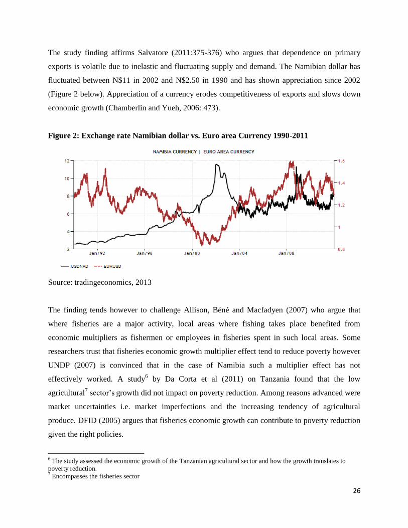
The study finding affirms Salvatore (2011:375-376) who argues that dependence on primary

exports is volatile due to inelastic and fluctuating supply and demand. The Namibian dollar has

fluctuated between N$11 in 2002 and N$2.50 in 1990 and has shown appreciation since 2002

(Figure 2 below). Appreciation of a currency erodes competitiveness of exports and slows down

economic growth (Chamberlin and Yueh, 2006: 473).

Figure 2: Exchange rate Namibian dollar vs. Euro area Currency 1990-2011

Source: tradingeconomics, 2013

The finding tends however to challenge Allison, Béné and Macfadyen (2007) who argue that

where fisheries are a major activity, local areas where fishing takes place benefited from

economic multipliers as fishermen or employees in fisheries spent in such local areas. Some

researchers trust that fisheries economic growth multiplier effect tend to reduce poverty however

UNDP (2007) is convinced that in the case of Namibia such a multiplier effect has not

effectively worked. A study6 by Da Corta et al (2011) on Tanzania found that the low

agricultural7 sector’s

growth did not impact on poverty reduction. Among reasons advanced were

market uncertainties i.e. market imperfections and the increasing tendency of agricultural

produce. DFID (2005) argues that fisheries economic growth can contribute to poverty reduction

given the right policies.

6 The study assessed the economic growth of the Tanzanian agricultural sector and how the growth translates to

poverty reduction. 7 Encompasses the fisheries sector

27

As expected and in accord with theory and previous empirical evidence, the study results reveal

that unemployment impacts negatively and with statistical significance on economic growth.

Unemployment is the second most important determinant of economic growth in Namibia during

1990-2011. Results show that unemployment tends to reduce economic growth as a unit increase

in unemployment seems to reduce economic growth nearly by 1%. Approximately 49% of house

of households in Namibia derive their incomes from wages or salaries and at the same time about

27% of the population is unemployed (NSA, 2012). The results suggest that by not making use

of its labour, inefficiency occurs leading to lower economic growth. The finding corroborates

that of Radvansky and Tiruneh (2011) who used panel data for the European Union 1995-2009

to investigate economic growth and human capital and found a positive statistically significant

relationship.

Results show, the model and thus the independent variables explain only 20.6% of the variations

in the economic growth leaving unexplained 79.4%. The model correlation coefficient8 (adjusted

R2) is 0.206 and statistically insignificant (see table 13 in the appendix).

Of the estimated independent variables i.e. initial per capita GDP, gross capital formation,

unemployment, general government expenditure and fisheries gross capital formation against

economic growth only unemployment and initial GDP are found to be statistically significant

determinants of economic growth in Namibia during 1990-2011.

Other basic per capita GDP growth model regression (equation 2)

To better understand the influence the fisheries sector has on economic growth, the same basic

per capita GDP growth equation is estimated without the fisheries per capita GDP variable. The

study has identified it a focus sector because of its importance in the economy. Additionally this

serves to further explore the effect other explanatory variables have on economic growth without

the fisheries per capita GDP influence. Explanatory variables in regressions sometimes tend to

8 (Gujarati and Porter, 2009: 243) noted that it is not strange for correlation coefficient (adjusted R

2) because of the

diversity nature of cross sectional data

28

influence other variables same way as economic sectors influence each other. The indirect

measures of fisheries might still be reflected by the estimated variables even though its direct

effect will not be picked up. The estimated outputs are presented in tables 14-16 in the appendix.

The estimated model:

Table 3: Other basic GDP growth estimated output: Fisheries variable omitted

Model Unstandardized Coefficients Standardized

Coefficients

t Sig.

B Std. Error Beta

1

(Constant) 3.799 1.705 2.228 .042

LAGlnCGDP -.375 .170 -3.036 -2.201 .044

GFCF GR .034 .042 .164 .809 .431

GVR G .052 .068 .169 .763 .457

UN GR -.068 .032 -.529 -2.111 .052

T .013 .007 2.694 1.959 .069

Dependent Variable: GDP GR

The findings show that initial per capita GDP and unemployment are negative and statistically

significant determinants of economic growth while gross fixed capital formation and government

expenditure are positive and not statistically significant determinants. The finding suggests that

even with the omission of the fisheries sector, the regression results maintain the status quo (as in

equation 1). The fisheries sector may still affect economic growth through the remaining

variables i.e. employment, government expenditure and gross capital accumulation and the result

suggest that its direct effect (measured by the fisheries variable in equation 1) on economic

growth might be nearly the same as its indirect effect.

One key finding that can be made between equations (1) and (2) is that the model correlation

coefficient did not change. This means that the four remaining variables (initial GDP, gross fixed

capital formation, government expenditure and unemployment in equation (2)) maintained the

same explanatory power of variation in economic growth and in fact holding them all constant,

the result suggests a higher economic growth than without the fisheries sector. The estimated

constant coefficient increased from 3.512 to 3.799 suggesting that ceteris paribus, on average

29

GDP growth tends to be higher with the exclusion of the fisheries sector. This result affirms the

finding of equation (1) that the fisheries sector’s impact on economic growth is statistically

insignificant.

With the fisheries sector inclusive, the findings show that the economic growth influence of

initial GDP increased (from -0.346 to -0.375) while reduced were that of unemployment (from -

0.072 to -0.068), government expenditure (from 0.072 to 0.052) and gross fixed capital

formation (from 0.04% to 0.034%). This implies that fisheries enhance initial GDP per capita,

government expenditure and gross fixed capital formation but not employment. Holding other

independent variables constant, the estimated coefficient of initial per capita GDP predicts higher

growth in response to lower initial GDP. It implies that a unit reduction in initial GDP will

increase the GDP growth by 0.38% on average per year. It would be interesting to find out how

fisheries and what type of government expenditure is enhanced as a result of fisheries influence.

Without fisheries, government expenditure tends to reduce and economic growth tends to

increase. This finding suggests that government spends more with inclusion of the fisheries

sector which tends to negatively affect economic growth than the counterfactual. The finding

supports the Ricardian view on government spending that argues against the role government can

play in determining economic growth since government expenditure is financed through taxes

and which if increased reduces disposable income for economic agents (Chamberlin & Yueh,

2006: 95) and might have negative repercussions for an economy characterized by poverty. Also

in agreement is Barro and Sala-i-Martin (2004: 526) who found that an increase in government

expenditure reduces economic growth.

Additionally, the findings suggest that without fisheries influence, unemployment is estimated to

be statistically significant at a significance level of 10% than at the previous 5%. The finding

suggests that for every 1% increase in unemployment, economic growth tends to reduce by

0.068% implying that the fisheries sector worsens employment rather than eases it. The negative

impact of unemployment on economic growth is less without the fisheries sector, suggesting that

the sector does indeed play a role in employment or equally in unemployment as the

unemployment effect increases when the fisheries sector comes into the picture.

30

5.2 The basic fisheries per capita GDP growth model (equation 3)

Data for the fisheries sector is investigated to establish what determined economic growth in the

sector during 1990-2011. Regression results of the fisheries GDP growth model are presented in

table 4 below. Descriptive statistics indicate that real fisheries economic growth rate fluctuated

between -2.42% and -4.64% and averaged at 4.7% per year. The correlation matrix for regressed

variables together with other regression outputs i.e. descriptive statistics is presented in the

appendix tables 17-20.

The estimated equation is:

Table 4: The basic fisheries per capita GDP growth model output

Model Unstandardized Coefficients Standardized

Coefficients

t Sig.

B Std. Error Beta

1

(Constant) 4.027 1.681 2.396 .031

LAGlnFGDP -.535 .238 -.879 -2.248 .041

FGFCF GR -.029 .020 -.344 -1.451 .169

GVR G .447 .428 .255 1.044 .314

UN GR .183 .222 .252 .823 .424

GFCF GR .219 .236 .186 .930 .368

T .007 .014 .242 .474 .643

Dependent Variable: FGDP GR

The findings suggest that economic growth of the fisheries sector most importantly depend on

initial fisheries per capita GDP, the only variable estimate that is statistically significant related

to fisheries per capita GDP growth. From the table above, it can be seen that the conditional

convergence hypothesis for the fisheries sector is supported, with a p value of 0.04, the estimated

coefficient -.535 (s.e 0.238). Holding other explanatory variables constant, the coefficient

predicts higher growth in response to lower initial fisheries per capita GDP growth. The

estimated coefficient shows the sector’s convergence rate is about 0.54% per year. Alternatively

it predicts that a dollar reduction in initial fisheries GDP tends to increase fisheries growth by

0.54% on average per year.

31

The estimated coefficient of fisheries gross fixed capital formation suggests that the sector’s

investments did not make a significant contribution to the sector’s growth during the period

under review. Holding other independent variables constant, the coefficient predicts a reduction

of 0.219% in the sector’s per capita GDP growth on average per year. This finding is against

theory and finding of Barro and Sala-i-Martin (2004) who found capital to positively correlate to

economic growth. Capital tends to have diminishing returns and extra units of it might be more

costly in terms of maintenance to keep them operational. This might contribute negatively to

growth.

The coefficient estimate of government expenditure is statistically insignificant in relation to

fisheries economic growth. The finding suggests that a unit increase in government expenditure

holding other independent variables increases growth rate by 0.4%. This implies that the more

government spends the higher the sector’s economic growth. The finding does not support the

Ricardian view. Furthermore, the results show a positive and statistically insignificant

relationship between unemployment and fisheries economic growth. This suggests that as

employment in the sector increases, its economic growth reduces. This implies that the Namibian

economy tends to not depend on the fisheries sector for employment. Unemployment generally

tends to reduce growth because factors of production are not utilised and efficiency is

compromised, however this is different for capital intensive fisheries sector. The estimated

coefficient suggests that for every 1% increase in unemployment, the fisheries economic growth

increases by 0.183% on average per year. The finding supports DFID (2005) who argue that

employment creation stops as the fisheries industry technologically progresses. In support is also

Allison (2011) who found that most jobs in capture fisheries are decreasing or stagnating

especially in capital intensive countries because of the capital intensity of fisheries9 or causes

like low catches, fishing capacity reduction plans and advanced technology. Allison further

argues that while capture fisheries employment decreases aquaculture increasingly provides

employment. Such a result might not be what an advocate for more employment would fancy to

see, more so definitely not for Namibia which is characterised by high poverty levels and high

unemployment. Hull (2009) argues that employment contributes to economic growth and poverty

9 Examples are Japan, North America and European countries

32

reduction as many people’s source of income is work. Furthermore argues that for employment

intensive economies to enhance economic growth and reduce poverty, employment should be

created in more productive sectors while less productive sectors require more productive growth.

Gutierrez et al. (2007) agrees that sectorial employment and intensities of production are crucial

for poverty reduction. In support, is also Adams (2003) whose study determined to what extent

economic growth reduces poverty for low income countries and found that economic growth

reduces poverty, that it provides more jobs for people to work and eventually raises income for

the members of society.

Furthermore, the results indicate that the estimated coefficient of gross fixed capital formation is

positively related to fisheries economic growth but statistically insignificant at 0.219 (0.236)

with p (0.368). A unit increase in gross fixed capital formation tends to increase fisheries

economic growth by 0.219%. This means that acquiring of equipment and other durables is

imperative for the sector’s growth.

Overall, the result show that the variables considered, after taking into consideration their

number, they are able to explain only 24.4% of the variations in the fisheries economic growth

leaving 76.6% unexplained (see Table 19 in the Appendix).

Other fisheries per capita GDP growth model (equation 4)

Regression results of the second regressed fisheries GDP growth model are presented in table 5

below. The rest of the output i.e. descriptive statistics are presented tables 21-23 in the

Appendix. The regression excluded the gross fixed capital formation with the purpose of

attempting to understand the growth rate of the sector while shielded from the influence of the

aggregate capital formation.

The estimated equation is:

33

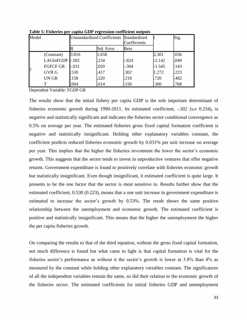
Table 5: Fisheries per capita GDP regression coefficient outputs

Model Unstandardized Coefficients Standardized

Coefficients

t Sig.

B Std. Error Beta

1

(Constant) 3.816 1.658 2.301 .036

LAGlnFGDP -.502 .234 -.824 -2.142 .049

FGFCF GR -.031 .020 -.364 -1.545 .143

GVR G .530 .417 .302 1.272 .223

UN GR .158 .220 .218 .720 .482

T .004 .014 .150 .300 .768

Dependent Variable: FGDP GR

The results show that the initial fishery per capita GDP is the sole important determinant of

fisheries economic growth during 1990-2011. Its estimated coefficient, -.502 (s.e 0.234), is

negative and statistically significant and indicates the fisheries sector conditional convergence as

0.5% on average per year. The estimated fisheries gross fixed capital formation coefficient is

negative and statistically insignificant. Holding other explanatory variables constant, the

coefficient predicts reduced fisheries economic growth by 0.031% per unit increase on average

per year. This implies that the higher the fisheries investment the lower the sector’s economic

growth. This suggests that the sector tends to invest in unproductive ventures that offer negative

returns. Government expenditure is found to positively correlate with fisheries economic growth

but statistically insignificant. Even though insignificant, it estimated coefficient is quite large. It

presents to be the one factor that the sector is most sensitive to. Results further show that the

estimated coefficient, 0.530 (0.223), means that a one unit increase in government expenditure is

estimated to increase the sector’s growth by 0.53%. The result shows the same positive

relationship between the unemployment and economic growth. The estimated coefficient is

positive and statistically insignificant. This means that the higher the unemployment the higher

the per capita fisheries growth.

On comparing the results to that of the third equation, without the gross fixed capital formation,

not much difference is found but what came to light is that capital formation is vital for the

fisheries sector’s performance as without it the sector’s growth is lower at 3.8% than 4% as

measured by the constant while holding other explanatory variables constant. The significances

of all the independent variables remain the same, so did their relation to the economic growth of

the fisheries sector. The estimated coefficients for initial fisheries GDP and unemployment

34

estimates showed relatively lower values that imply reduced impacts on fisheries growth when

therefore holding other independent variables constant. This suggests that, the gross investment

in the economy triggers unemployment in the fisheries sector (unemployment to increase as

without gross fixed capital formation, the estimated unemployment coefficient is lower) but

seems to boost the sector’s economic growth. Gross fixed capital formation seems to reduce

government expenditure for without it government expenditure shows a higher estimated

coefficient (0.447 to 0.530). Results also show that the individual impact of fisheries capital

formation reduced and government expenditure on fisheries economic growth and increased

while other independent variables are held constant. The result suggests that the fisheries sector

is capitalized with capital that results in negative productivity of the sector. This state of affairs

seems to be negated by gross fixed capital formation as the estimated coefficient of fisheries

fixed capital formation shows a reduction from -0.029 to -0.031. This therefore suggests that

gross fixed capital formation enhances unemployment; fisheries fixed capital formation and

reduce initial fisheries GDP and government expenditure respectively.

Results suggest that gross fixed capital formation impacts positively on economic growth despite

its tendency to increase unemployment. The results do not support poverty reduction plans.

They do however support (Cypher and Dietz, 2004) on their argument that dependence on capital

intensive means for a country’s extraction of natural resources such as fisheries additionally

worsens poverty.

The result suggests that if the fisheries sector’s economic growth is to improve, its employment

should be lower, government expenditure should be higher, fisheries fixed capital formation

should be lower, gross fixed capital formations should be higher and initial fisheries per capita

should be lower.

5.3 HYPOTHESES TESTING RESULTS

The identified hypotheses are tested against the null hypothesis that economic growth and the

respective selected independent variables (initial GDP, gross fixed capital formation and

unemployment) economic growth are independent. The alternative hypothesis assumes linear

35

dependence between economic growth and the respective independent variables. Using bivariate

analysis the hypotheses were tested. Regression outputs are presented in Appendix, tables 24-36.

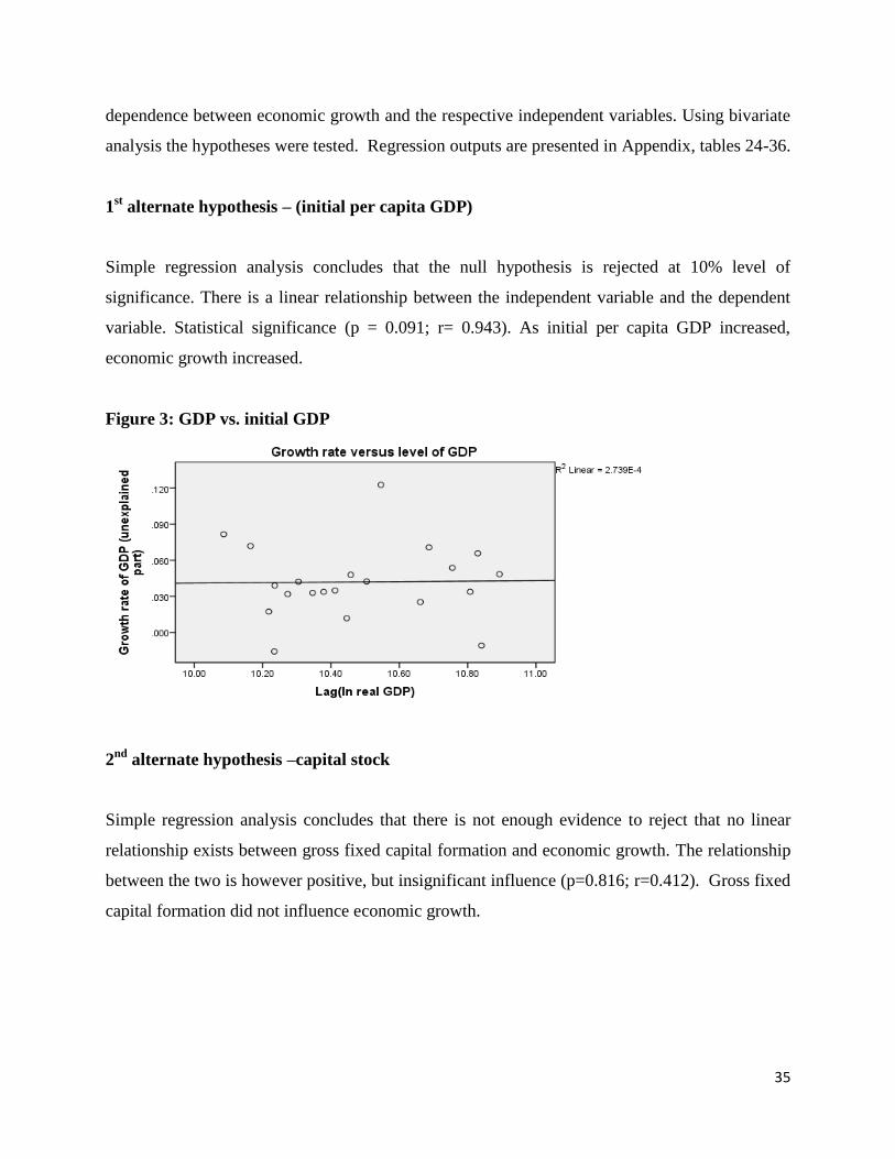
1st alternate hypothesis – (initial per capita GDP)

Simple regression analysis concludes that the null hypothesis is rejected at 10% level of

significance. There is a linear relationship between the independent variable and the dependent

variable. Statistical significance (p = 0.091; r= 0.943). As initial per capita GDP increased,

economic growth increased.

Figure 3: GDP vs. initial GDP

2nd

alternate hypothesis –capital stock

Simple regression analysis concludes that there is not enough evidence to reject that no linear

relationship exists between gross fixed capital formation and economic growth. The relationship

between the two is however positive, but insignificant influence (p=0.816; r=0.412). Gross fixed

capital formation did not influence economic growth.

36

Figure 4: Gross fixed capital formation versus GDP growth

3rd

alternate hypothesis – unemployment

Simple regression analysis concludes that the null hypothesis is rejected. There is a linear

relationship between unemployment and economic growth. Statistical significance (p=0.044;

r=0.061). As unemployment increased, economic growth reduced.

Figure 5: GDP growth versus unemployment

Three of the two study hypotheses are confirmed to be of significance. Unemployment and initial

GDP but gross fixed capital formation is confirmed to be determinants of economic growth in

Namibia.

37

CHAPTER 6

CONCLUSIONS AND RECOMMENDATIONS

6.1 SUMMARY

The results indicate that Namibia’s economic growth has shown a positive average trend over the

years. The economy’s per capita GDP growth averaged 4.4% while the fisheries sector averaged

4.7% per year during 1990-2011. This implies that Namibia should ideally not have poor people

because of its high per capita GDP. Conditional convergence is found for the fisheries sector and

for the economy. Hence its role is found to be the most important determinant of economic

growth.

The fisheries sector's economic growth during 1990-2011 is determined by initial GDP.

Estimated factors of unemployment, fisheries fixed capital formation; gross fixed capital

formation and general government expenditure are not found to be statistically significant factors

of the sectors economic growth during the same period. The findings suggest a positive

relationship between unemployment and the sectors economic growth which implies that as the

sector employs more people its productivity reduces and hence economic growth reduces.

Figure 6: Relationship of fisheries growth (per capita GDP) vs. unemployment

38

Therefore, the study does not find significant statistical evidence to support that the sector

directly affects unemployment. This implies that employment, a means through which most of

the country's citizens derive income is not positively influenced by the fisheries sector, leading to

a conclusion that the sector does not positively and significantly impact on poverty reduction.

The sector’s economic growth is positively correlated with unemployment and negatively

correlated with the country’s economic growth. The findings thus do not suggest enough

evidence to advocate that the sector impacts positively on employment and economic growth.

Additionally, the study does not find enough evidence to suggest that the fisheries sector

determines economic growth in Namibia. This fact also dismisses statistical significance of the

direct impact on economic growth of the sector including its revenue contribution to the state.

The results suggest that Namibia’s economic growth is determined by initial GDP and

unemployment. Both the factors have a negative and statistical significant relationship with the

country’s economic growth. The findings imply that the economy is not creating sufficient job

opportunities. Other factors: gross fixed capital formation and government expenditure estimated

for influence on economic growth are found to be of no important prediction.

Two of the three hypotheses tested correlating unemployment, initial GDP, gross fixed capital

formation against economic growth also showed statistical significance confirming

unemployment and initial GDP as determinants of economic growth in Namibia. Capital

formation though proven through empirical evidence and acclaimed by development theorists as

one of the most important determinants of economic growth, evidence from this study does not

support the acclamation. It is possible that the type of data collected, or the procedure used to

give meaning to this variable, has several shortcomings that might have influenced its credibility

but findings on unemployment and initial GDP per capita were reasonably in line with those of

other studies and theory thus leaving little room to assume this for capital formation.

The study did not find evidence to support that fisheries economic growth directly reduces

poverty in Namibia. The fisheries sector may not be of statistical significance to the economy;

nevertheless considering the fact that more than 49% of the population in Namibia derive their

39

income from wages and that an average household in Namibia has 4.7 people, assuming that the

12825 people employed in the fisheries sector head households, this can be inferred to mean

60277 people’s (approximately 3% of the population) standard of living depends on the fisheries

sector. The number may seem little but it may reduce the number of people below the poverty

line.

The results reveal policy implication that Namibian economic growth seems to be employment

driven and thus enhancing employment tends to boost the country’s economic growth. Namibian

policy makers are challenged to devise strategies that enhance employment creation

opportunities and reduce initial per capita GDP. The result revealed that capital formulation is

not a determinant of Namibian economic growth during the period under review. Capital

formation determines convergence. It is therefore evident that if Namibia wishes to enhance its

economic growth and reduce poverty, that it may consider to create employment opportunities,

reduce initial per capita GDP, invest in the right capital, and increase economic growth of the

fisheries sector. Furthermore, if the fisheries sector, through its economic growth, is to reduce

poverty, policy makers may wish to most importantly design strategies that reduce the sector's

initial GDP, increase government expenditure, reduce employment and increase gross fixed

capital formation and make it conducive for the sector to reduce its sectorial capital formation

without losing productivity.

6.2 CONCLUSIONS

The purpose of the study is to determine if economic growth, with particular emphasis on the

fisheries sector, impacts on poverty reduction during the period of 1990-2011. The study

investigates factors that determine the fisheries sector economic growth parallel to the aggregate

economy’s growth. To explain the variation and better understand the economic growth and

whether it reduces poverty, economic growth determining factors i.e. initial per capita GDP,

gross fixed capital formation, fisheries growth, general government expenditure: income,

expenditure & savings and unemployment are analysed using the neoclassical model framework.

40

The results reveal that Namibian economic growth during the period studied is explained by

conditional convergence and unemployment as the most important determinants. Gross fixed

capital formation, government expenditure and the fisheries sector are not found to be significant

determinants of Namibia’s growth. The findings suggest that the economy is not creating

sufficient job opportunities. Despite the economy’s constant dependence on the fisheries sector

for its exports the study results suggests that the sector is not an important determinant of

Namibia’s economic growth. The finding on government spending suggests that the more

government spends the higher the economic growth and this does not support the Ricardian

theoretical view on government expenditure.

The results of the fisheries sector revealed that the sector’s economic growth is determined by

initial GDP thus conditional convergence is found. Fisheries fixed capital formation; general

government expenditure, unemployment and gross fixed capital formation are revealed not to

statistically significantly determine fisheries economic growth during the period studied. Unlike

the negative relationship found between the aggregate economy and unemployment, the

relationship between unemployment and the fisheries sector is positive, which suggests that the

higher the employment in the fisheries sector, the lower the sector’s economic growth. The

results also suggest that the more the sector invests in capital, the lower its economic growth.

The results present policy implications that if policy makers desire to increase the sector’s

economic growth and consequently the sectors contribution to the country’s economic growth

that they may have to increase government expenditure, increase gross fixed capital formation,

reduce initial GDP, allow for employment reduction in the sector and reduce fisheries gross fixed

capital formation.

The study finds no evidence to suggest that the fisheries sector’s economic growth impacts to

reduce poverty either on its own through the sectorial employment or through the sector’s

contribution to aggregate economic growth. For, as the sector’s employment increases, the

sector’s economic growth reduces, reducing the sector’s ability to directly reduce poverty

through employment. Additionally the sector’s economic growth correlates negatively to the

country’s economic growth.

41

The findings support Allison, Béné and Macfadyen, (2007) that fisheries contribution towards

poverty reduction will be complementary to overall national poverty reduction efforts as the

fisheries sector is minor and its contribution alone is not sufficient to counteract poverty. Policy

implications for the aggregate economy as inferred from the results are similarly that if the

policy makers wish to enhance economic growth of the country they may have to reduce initial

GDP, increase government expenditure, reduce unemployment, increase gross fixed capital

formation, increase growth of the fisheries sector and increase gross fixed capital formation. This

goes without saying; an enhanced economic growth presents great potential for poverty

reduction.

As noted by Grindle (2007) poverty reduction depends on the government’s level of

reinvestment of the revenues from the sector into public goods and creation of employment in

the economy, the degree of which is greatly determined by public policy. Adam Smith once

stated that people are the wealth of nations and Namibia ought to appropriate them efficiently for

the benefit of the economy. People are the creators of wealth but only provided they are given an

opportunity.

The study revealed that there are other determinants that enhance economic growth other than

the ones investigated in this study. This implies the importance to policy makers that such

determinants are identified and investigated. A better understanding of such factors is vital for

policy formulations to enhance economic growth and reduce poverty.

6.3 RECOMMENDATIONS FOR FUTURE RESEARCH

For future research, other researchers could replicate the study focusing on other sectors of the

economy. That would make an interesting finding while at the same time contributing to the

body of available literature. This study is limited to the fisheries sector.

The results indicate that there are factors that enhance economic growth be it for the fisheries

sector or economy that are not explained by the study. It is important that these factors are

identified and investigated for better policy formulation. Other researchers may consider this.

42

Last but not least, a study on the indirect impact of fisheries in the economy i.e. downstream-

upstream industry trickle effect and economic growth would be interesting.

43

REFERENCES

Adams. R. H., 2003. Economic growth, Inequality and Poverty: Findings from a new data set.

[online] Available at: <http://www-wds.worldbank.org/externatl/default/wdscontentserver/sdsp/i

b/2003/03/22/000094946_03030704153293/rendered/pdf/multi0page.pdf[accessed> [Accessed

on on 3 July 2013].

Acemoglu, D. Johnson, S. and Robinson, J.A., 2001. The Colonial Origins of Comparative

Development: An Empirical Investigation. [online] Available at: <http://economics.mit.edu/files/

4123 > [Accessed on 3 March 2013].

Allison, E., 2011. Aquaculture, Fisheries, Poverty and Food Security. [online] Available at:

<http://www.worldfishcenter.org/resource_centre/WF_2971.pdf>[Accessed on 3 May 2013].

Allison, E.H., Béné, C.M. and Macfadyen, G., 2007. Increasing the contribution of small-scale

fisheries to poverty alleviation and food security. [online] Rome, FAO. Available at:

<http://www.cbd.int/doc/books/2009/B-03165.pdf > [Accessed 25 May 2013].

Amunkete. T. and Nyambe. J.M., 2009. Small-Scale Mining and its impact on poverty in

Namibia: A case study of miners in the Erongo Region. [online]. Available at:

<http://www.tips.org.za/files/SSM_NEPRU_project_Final.pdf > [Accessed on 24 June 2013].

Arthur, R. Fisher. E. Irz, X. Mwaipopo, R. and Thirtle. C., 2005. Fisheries Management Science

Programme: An overview of developmental impact to 2005. [online]. Available at:

<http://www.fmsp.org.uk/Documents/r4778c/R4778C_FTR.pdf> [Accessed 6 December 2012].

Ashipala, M.J. and Eita, J.H., 2010. Estimating Namibia’s export potential: A gravity model

approach. [online] Available at: <http://www.undp.org.na/SharedFiles/Download.aspx?pageid=4

4&fileid=128&mid=84> [Accessed on 3 June 2013].

44

Ashipala, M.J. and Eita, J.H., 2010. Determinants of unemployment in Namibia. [online]

Available at: <http://ccsenet.org/journal/index.php/ijbm/article/download/7635/5864>[Accessed

on 30 June 2013].

Barro, R.J., 1996. Determinants of Economic Growth: A Cross-Country Empirical

Study. [online] Available at: <http://www.nber.org/papers/w5698.pdf?new_window=1> [Access

ed 6 June 2013].

Barro, R. and Sala-i-Martin, X., 2nd

edition. 2004. Economic Growth, Cambridge. MIT Press.

Beard, T.R. Ford, G.S. Kim, H. and Spiwak, L.J., 2011. Regulatory expenditures, economic

growth and jobs: An empirical study. [Online] Available at: <http://www.phoenix-center.org/Pol

icyBulletin/PCPB28Final.pdf> [Accessed 13 June 2013].

Bell, E. and Bryman, A., 3rd

edition. 2007. Business Research Methods. Oxford. Oxford

University Press.

Berenson, M.L. Levine, M.D. Krehbiel, C.T. and Stephan, D.F., 6th

edition. 2011. Statistics for

managers: Using Microsoft Excel. Harlow. Pearson.

BON, 2010. Annual report 2010. [online] Available at: <https://www.bon.com.na/CMSTemplate

s/Bon/Files/bon.com.na/81/8101f8ed-83d1-4350-9edd-e9a979eb2532.pdf> [Accessed on 3

March 2013]

BON, 2012. Quarterly Bulletin. [Online] Available at: <http://www.bon.com.na> [Accessed 6

March 2013].

Chamberlin, G. and Yueh, L., 2006. Macroeconomics. London: Thomas Learning.

45

CIA, 2012. The World Factbook. [Online]. Central Intelligence Agency. Available at:

<https://www.cia.gov/library/publications/the-world-factbook/geos/wa.html> [Accessed on 17

December 2012].

Chong, K., 1993. Labour absorption in fisheries: Inevitable trends and prospects in employment

creation. [online] Available at: <http://www.apfic.org/archive/symposia/1993/03.pdf> [Accessed

10 May 2013].

Cypher, M.J. and Dietz, J.L., 2004. The process of Economic Development. Wiltshire.

Routledge.

Da Corta, L. Maro., F. Mashindano, O. and Kayunze, K., 2011. Agricultural growth and poverty

reduction in Tanzania 2000-2010: where has agriculture worked for the poor and what can we

learn from this? [online] Available at: <http://www.chronicpoverty.org/uploads/publication_files

/WP208%20Mashindano%20et%20al.pdf> [Accessed 10 May 2013].

DFID, 2005. The Role of Fisheries in Economic Growth and Poverty Alleviation <http://transpar

entsea.co/images/a/ad/Keysheetfishpovgrowth2005.pdf> [Accessed 10 July 2013].

Eita, J.H. and Jordaan. A.C., 2007. Export and economic growth in Namibia: A granger

causality analysis. [online]. Available at: <http://repository.up.ac.za/bitstream/handle/2263/4041/

Jordaan_Export(2007).pdf?sequence=1>[Accessed 6 July 2013].

FAO, 2012. The state of world fisheries and aquaculture. Food and Agriculture Organization.

Rome. [online] Available at: <http://www.fao.org/docrep/016/i2727e/i2727e.pdf> [Accessed on

26 June 2013].

FMSP, 2012. Fisheries and Poverty Reduction. [Online]. Available at:

<http://www.mrag.co.uk/Documents/PolicyBrief1_Poverty_Reduction.pdf> [Accessed on 11

November 2012].

46

Gerlagh, R. and Papyrakis. E., 2004. The resource curse hypothesis and its transmission

channels. [online] Available at: <http://www.uea.ac.uk/polopoly_fs/1.146885!Resource_curse_g

rowthjce30[1].pdf> [Accessed 18 July 2013].

Gerlagh, R. and Papyrakis. E., 2007. Resource Abundance and Economic Growth in the United

States. [online] Available at: <http://www.uea.ac.uk/polopoly_fs/1.146883!Abundance_resource

-americas79eer%5B1%5D.pdf>[Accessed 12 July 2013].

Godana, T. and Odada, J.E., 2002. Sources of growth in Africa: A case study of Namibia.

[online] Available at: <http://www.gpean.org/aaps/Namibia-OdadaFR.pdf> [Accessed 6 July

2013].

Grindle, M.S., 2007. Good Enough Governance Revisited. [online] Available at:

<http://relooney.fatcow.com/00_New_1805.pdf> [Accessed 11 July 2013].

Gujarati, D.N. and Porter, D.C., 5th

edition. 2009. Basic Econometrics. Mc Graw Hill. New

York.

Gutierrez, C. Orecchia. C. Paci. P. and Serneels, P., 2007. Does Employment Generation Really

Matter for Poverty Reduction? [online] Available at:

<http://www-wds.worldbank.org/servlet/WDSContentServer/WDSP/IB/2007/12/06/000158349_

20071206131549/Rendered/PDF/wps4432.pdf> [Accessed 12 July 2013].

Huggins and Izushi., 2004. Empirical analysis of human capital development and economic

growth in the European regions. [online] Available at:

<http:www.cedefop.europa.eu/EN/Files/BgR3_Izushi.pdf> [Accessed 10 July 2013].

Hull, K., 2009. Understanding the Relationship between Economic Growth, Employment and

Poverty Reduction [online] Available at: <http://www.oecd.org/dac/povertyreduction/43280288.

pdf> [Accessed 10 March 2013].

47

Knowles, S., 2011. Inequality and Economic Growth: The empirical relationship reconsidered

in the light of comparable data. [online] Available at: <http://www.nottingham.ac.uk/credit/docu

ments/papers/01-03.pdf> [Accessed on 3 March 2013].

Kurien, J., 2004. Responsible fish trade and Security: Report on the Impact of International

Trade in fishery products on food security. [Online] Available at:

<http://www.tradefoodfish.org/images/iitfpfs2.PDF > [Accessed on 3 December 2012].

Lange, G.M., 2003. National wealth, natural capital and sustainable development in Namibia.

[online] Available at: <http://www.the-eis.com/data/RDPs/RDP56.pdf> [Accessed on 3 July

2013].

Lange, G.M. and Motinga, D.J., 1997. The Contribution of Resource Rents from Minerals and

Fisheries to Sustainable Economic Development in Namibia. [online] Available at:

<http://millenniumindicators.un.org/unsd/envaccounting/ceea/archive/Fish/Namibia_ResourceRe

nt_Fisheries_Minerals.PDF> [Accessed 10 March 2013].

Ledyaeva, S. and Linden, M., 2006. Determinants of Economic Growth: Empirical Evidence

from Russian Regions. [online]. The European Journal of Comparative Economics. Available at:

<http://eaces.liuc.it/18242979200801/182429792008050105.pdf> [Accessed on 23 June 2013].

Levine, R., 1998. Book Reviews. [online]. Journal of Comparative Economics. Available at:

<http://www.econ.brown.edu/fac/Ross_Levine/Publication/1998_Review_JCE_Barro.pdf>

[Accessed on 22 June 2013].

Levine, S. and Roberts, B., 2008. Dynamics of income inequality and poverty in post-

independence Namibia. [online] Available at: <http://www.hsrc.ac.za/Research_Publication-

20799.phtml> [Accessed on 22 February 2013].

MFMR, 2009. From exploitation to sustainability: The journey of Namibia’s fisheries sector

since 1990. Windhoek, Ministry of Fisheries and Marine Resources.

48

MFMR, 2011. Annual Report 2010/11. [online] Available at: <http://www.mfmr.gov.na/>

[Accessed 15 June 2013].

MFMR, 2013. Statistics. [online] Available at: <http://www.mfmr.gov.na/> [Accessed 10 March

2013].

MOF, 2012. Statement for 2012/2013 Budget. [online]. Windhoek. Ministry of Finance.

Available at: <http://www.mof.na/index.html> [Accessed on 3 June 2013].

MOL, 2013. Namibia Occupational Wages Survey (NOWS) 2009. [online]. Windhoek. Ministry

of Labour. Available at: < http://www.mol.gov.na/> [Accessed on 4 March 2013].

NPC, 2007. An analysis of the economic challenges of Namibia and how the Donor Community

should assist. [online] Windhoek. National Planning Commission. Available at: <

http://www.npc.gov.na/publications/EconomicChallengesofNamibia.pdf> [Accessed 3 May

2013].

NPC, 2011. Namibia 2011 population and housing census preliminary results. [Online]

Available at: <http://www.npc.gov.na/publications/2011_Preliminary_Result.pdf> [Accessed on

4 November 2012].

NPC, 2011. Targeted Intervention Program for Employment and Economic and Economic

growth. [Online] Available at: <http://www.npc.gov.na/publications/TIPEEG.pdf> [Accessed on

9 November 2012].

NPC, 2012. Republic of Namibia - Namibia’s Fourth National Development Plan 4: 2012/13 to

2016/17. [Online] Available at: <http://www.npc.gov.na/npc/ndp4info.html> [Accessed 12

December 2012].

NSA, 2012. Namibia Household Income and Expenditure Survey 2009/2010. [online] Available

at: <http://www.nsa.org.na/publications/> [Accessed 10 March 2013].

49

NSA, 2012. Poverty Dynamics in Namibia: A comparative study using the 1993/94, 2003/04

and the 2009/10 NHIES surveys. [online] Available at: <http://www.nsa.org.na/files/downloads/

b51_Poverty%20Dynamics%20Report%20in%20Namibia.pdf>[Accessed 12 February 2013].

Pegg, S., 2003. Poverty Reduction or Poverty Exacerbation? [online] Available at:

<http://commdev.org/files/1867_file_pegg.pdf > [Accessed 10 March 2013].

Radvansky, M. and Tiruneh, M.W., 2011. The Contribution of Human capital to European

Economic Growth: An empirical exploration from a panel data. [Online] Available at:

<http://ecomod.net/system/files/Tiruneh_Radvansky_Ecomod2011_1.pdf>[Accessed on 19 June

2013].

RIU, 2012. Managing fisheries when there is not much data. [Online]. Available at:

<http://researchintouse.com/nrk/RIUinfo/PF/FMSP06.htm#L5> [Accessed 11 November 2012].

Salvatore, D., 10th

edition. 2011. International Economics: Trade and Finance. Hoboken. John

Wiley and Sons Inc.

Seligson, A.M. and Passé-Smith, J.T., 4th

edition. 2008. Development and Under Development:

The Political Economy of Global Inequality. London. Lynne Rienner Publishers Inc.

Solow, R.M. 1986. On the Intergenerational Allocation of Natural Resources. [Online].

Available at: <http://www.radford.edu/~gsantopi/nrem/solow%20resources.pdf>[Accessed 27

July 2013].

Soy, S.K., 1997. The Case Study as a Research Method. [Online]. Available at:

<http://www.gslis.utexas.edu/~ssoy/usesusers/l391d1b.htm>[Accessed 27 November 2012].

Tradingeconomics, 2013. Namibian Dollar. [online] Available at: <http://www.tradingeconomic

s.com/namibia/currency> [Accessed on 3 March 2013].

50

UNDP, 2007. [online] Available at: Economic Review. <http://www.undp.org.na/SharedFiles/Do

wnload.aspx?pageid=44&fileid=127&mid=84>[Accessed on 23 February 2013].

UNDP, 2013. Human Development Report 2013. [online] Available at:

<http://hdr.undp.org/en/statistics/hdi/> [Accessed on 19 February 2013].

UNDP, 2013. Understanding Poverty and Inequality in Namibia. [online] Available at: <

http://www.undp.org/content/undp/en/home/ourwork/povertyreduction/projects_and_initiatives/p

rojects_namibia/ > [Accessed on 23 February 2013].

Walliman, N., 2nd

edition. 2005. Your research project. Great Britain. The Alden Press.

Wong, K., 1993. Labour absorption in fisheries: Inevitable trends and prospects in employment

creation. [online] Available at: <http://www.apfic.org/archive/symposia/1993/03.pdf >[Accessed

on 3 December 2012].

World Bank, 2008. The Growth Report: Strategies for Sustained Growth and Inclusive

Development. Commission on Growth and Development, The International Bank for

Reconstruction and Development/The World Bank. [online] Available at: <http://www-

wds.worldbank.org/external/default/WDSContentServer/WDSP/IB/2008/08/20/000334955_2008

0820065406/Rendered/PDF/449860PUB0Box3101OFFICIAL0USE0ONLY1.pdf>[Accessed on

3 December 2012].

World Bank, 2013. Income inequality. [online] Available at: <http://www.worldbank.org/depwe

b/beyond/beyondco/beg_05.pdf > [Accessed on 6 March 2013].

World Bank, 2013. Namibia Overview. [online] Available at: <http://www.worldbank.org/en/cou

ntry/namibia/overview> [Accessed 5 March 2013].

51

APPENDICES

Table 6: All variable correlation matrix for per capita GDP growth basic model GDP

GR

lnCGDP GFC

F GR

GVR G FGDP

GR

UN GR lnEL

EC

lnTEL lnMOR

TAL

lnIMPSANI

T

lnEXPOINDX

GDP GR

Pearson

Correlation 1 .024 .050 .182 -.154 -.340 .158 -.079 .029 -.058 -.056

Sig. (2-

tailed)

.916 .824 .417 .493 .121 .483 .726 .897 .804 .804

N 22 22 22 22 22 22 22 22 22 21 22

lnCGDP

Pearson

Correlation .024 1 .133 .386 -.268 -.626

** .632

** .933

** -.994

** .974

** .989

**

Sig. (2-

tailed) .916

.554 .076 .228 .002 .002 .000 .000 .000 .000

N 22 22 22 22 22 22 22 22 22 21 22

GFCF

GR

Pearson

Correlation .050 .133 1 .104 .198 -.047 .058 .136 -.096 .201 .117

Sig. (2-

tailed) .824 .554

.644 .377 .835 .798 .547 .670 .383 .605

N 22 22 22 22 22 22 22 22 22 21 22

GVR G

Pearson

Correlation .182 .386 .104 1 .142 -.290 .417 .288 -.371 .290 .345

Sig. (2-

tailed) .417 .076 .644

.527 .191 .053 .194 .089 .202 .116

N 22 22 22 22 22 22 22 22 22 21 22

FGDP

GR

Pearson

Correlation -.154 -.268 .198 .142 1 .076 -.227 -.252 .283 -.402 -.292

Sig. (2-

tailed) .493 .228 .377 .527

.737 .309 .258 .203 .070 .188

N 22 22 22 22 22 22 22 22 22 21 22

UN GR

Pearson

Correlation -.340 -.626

** -.047 -.290 .076 1 -.299 -.477

* .613

** -.508

* -.597

**

Sig. (2-

tailed) .121 .002 .835 .191 .737

.177 .025 .002 .019 .003

N 22 22 22 22 22 22 22 22 22 21 22

lnELEC

Pearson

Correlation .158 .632

** .058 .417 -.227 -.299 1 .492

* -.609

** .556

** .601

**

Sig. (2-

tailed) .483 .002 .798 .053 .309 .177

.020 .003 .009 .003

N 22 22 22 22 22 22 22 22 22 21 22

lnTEL

Pearson

Correlation -.079 .933

** .136 .288 -.252 -.477

* .492

* 1 -.953

** .973

** .944

**

Sig. (2-

tailed) .726 .000 .547 .194 .258 .025 .020

.000 .000 .000

N 22 22 22 22 22 22 22 22 22 21 22

lnMORT

AL

Pearson

Correlation .029 -.994

** -.096 -.371 .283 .613

**

-

.609**

-.953

** 1 -.987

** -.994

**

Sig. (2-

tailed) .897 .000 .670 .089 .203 .002 .003 .000

.000 .000

N 22 22 22 22 22 22 22 22 22 21 22

lnIMPSA

NIT

Pearson

Correlation -.058 .974

** .201 .290 -.402 -.508

* .556

** .973

** -.987

** 1 .981

**

Sig. (2-

tailed) .804 .000 .383 .202 .070 .019 .009 .000 .000

.000

N 21 21 21 21 21 21 21 21 21 21 21

lnEXPOI

NDX

Pearson

Correlation -.056 .989

** .117 .345 -.292 -.597

** .601

** .944

** -.994

** .981

** 1

Sig. (2-

tailed) .804 .000 .605 .116 .188 .003 .003 .000 .000 .000

N 22 22 22 22 22 22 22 22 22 21 22

**. Correlation is significant at the 0.01 level (2-tailed).

*. Correlation is significant at the 0.05 level (2-tailed).

52

Table 7: All variable correlation matrix for per capita GDP growth basic model Correlations

FGDP

GR

LAGlnF

GDPGR

FGFCF

GR

GVR G UN GR GFCF

GR

LAGlnE

LEC

LAGlnT

EL

LAGlnM

ORTAL

LAGlnIM

PSANIT

LAGlnEXP

OINDX

FGDP GR

Pearson

Correlation 1 -.243 .014 .142 .076 .198 -.452* -.294 .318 -.310 -.295

Sig. (2-

tailed)

.471 .952 .527 .737 .377 .040 .196 .160 .172 .194

N 22 11 22 22 22 22 21 21 21 21 21

LAGlnFGDPGR

Pearson

Correlation -.243 1 -.700* -.360 .041 -.156 -.139 .458 -.374 .383 .379

Sig. (2-

tailed) .471

.017 .277 .905 .648 .666 .134 .231 .244 .224

N 11 12 11 11 11 11 12 12 12 11 12

FGFCF GR

Pearson

Correlation .014 -.700* 1 .149 .214 -.217 -.204 -.493* .417 -.417 -.422

Sig. (2-

tailed) .952 .017

.508 .340 .332 .376 .023 .060 .060 .057

N 22 11 22 22 22 22 21 21 21 21 21

GVR G

Pearson

Correlation .142 -.360 .149 1 -.290 .104 .227 .340 -.413 .391 .424

Sig. (2-

tailed) .527 .277 .508

.191 .644 .321 .132 .063 .080 .055

N 22 11 22 22 22 22 21 21 21 21 21

UN GR

Pearson

Correlation .076 .041 .214 -.290 1 -.047 -.301 -.503* .625** -.573** -.595**

Sig. (2-

tailed) .737 .905 .340 .191

.835 .185 .020 .002 .007 .004

N 22 11 22 22 22 22 21 21 21 21 21

GFCF GR

Pearson

Correlation .198 -.156 -.217 .104 -.047 1 -.095 -.007 .026 -.044 -.041

Sig. (2-

tailed) .377 .648 .332 .644 .835

.683 .977 .910 .849 .858

N 22 11 22 22 22 22 21 21 21 21 21

LAGlnELEC

Pearson

Correlation

-

.452* -.139 -.204 .227 -.301 -.095 1 .492* -.609** .556** .601**

Sig. (2-

tailed) .040 .666 .376 .321 .185 .683

.020 .003 .009 .003

N 21 12 21 21 21 21 22 22 22 21 22

LAGlnTEL

Pearson

Correlation -.294 .458 -.493* .340 -.503* -.007 .492* 1 -.953** .973** .944**

Sig. (2-

tailed) .196 .134 .023 .132 .020 .977 .020

.000 .000 .000

N 21 12 21 21 21 21 22 22 22 21 22

LAGlnMORTAL

Pearson

Correlation .318 -.374 .417 -.413 .625** .026 -.609** -.953** 1 -.987** -.994**

Sig. (2-

tailed) .160 .231 .060 .063 .002 .910 .003 .000

.000 .000

N 21 12 21 21 21 21 22 22 22 21 22

LAGlnIMPSANI

T

Pearson

Correlation -.310 .383 -.417 .391 -.573** -.044 .556** .973** -.987** 1 .981**

Sig. (2-

tailed) .172 .244 .060 .080 .007 .849 .009 .000 .000

.000

N 21 11 21 21 21 21 21 21 21 21 21

LAGlnEXPOIN

DX

Pearson

Correlation -.295 .379 -.422 .424 -.595** -.041 .601** .944** -.994** .981** 1

Sig. (2-

tailed) .194 .224 .057 .055 .004 .858 .003 .000 .000 .000

N 21 12 21 21 21 21 22 22 22 21 22

*. Correlation is significant at the 0.05 level (2-tailed).

**. Correlation is significant at the 0.01 level (2-tailed).

53

Table 8: Series of variables collected

Variables Symbols Mean (SD) Period

Gross Fixed capital formation by fishing (N$

millions), current

GFCFF 127.2273 1990-2011

General GVR expenditure: Income, EXP &

Savings (N$ million)

GGEI 12063.32 1990-2011

Gross Fixed capital formation, current GFCF 7610.318 1990-2011

Changes in inventories, current CII 35.5 1990-2011

GDP at Current prices GDP 36311.14 1990-2011

GDP at constant prices CGDP 37564.41 1990-2011

Unemployment rate (%) UN R 37.33182 1990-2011

GDP by activity Fishing and fish processing on

board

GDP FFOB 3.64135 1990-2011

GDP by activity (Current Prices) Fishing and fish

processing on shore

GDP FFOS 1.711006 1990-2011

Communications, computer, etc. (% of service

imports, BOP)

% SI BOP 2.66 1990-2011

Electricity production (kWh) ELEC 1.35 1991-2011

Mobile cellular subscriptions MOB 567915.1 1995-2011

Telephone lines TEL 109693.4 1990-2011

Internet users (per 100 people) INTERN 3.719437 1995-2011

Number of neonatal deaths NEO DEA 1272.727 1990-2011

Mortality rate, neonatal (per 1,000 live births) MORTAL 23.59091 1990-2011

Improved sanitation facilities (% of population

with access)

IMP SANIT 28.14286 1990-2010

Labor force, total LAB FO 675645.2 1990-2011

Mortality rate, infant (per 1,000 live births) MORTAL R 43.87727 1990-2011

Population, total POP 1889863 1990-2011

Export value index (2000 = 100) EXP IND 143.8131 1990-2011

Exchange rate N$ to US$ EXR 5.945411 1990-2011

Source: compiled by author

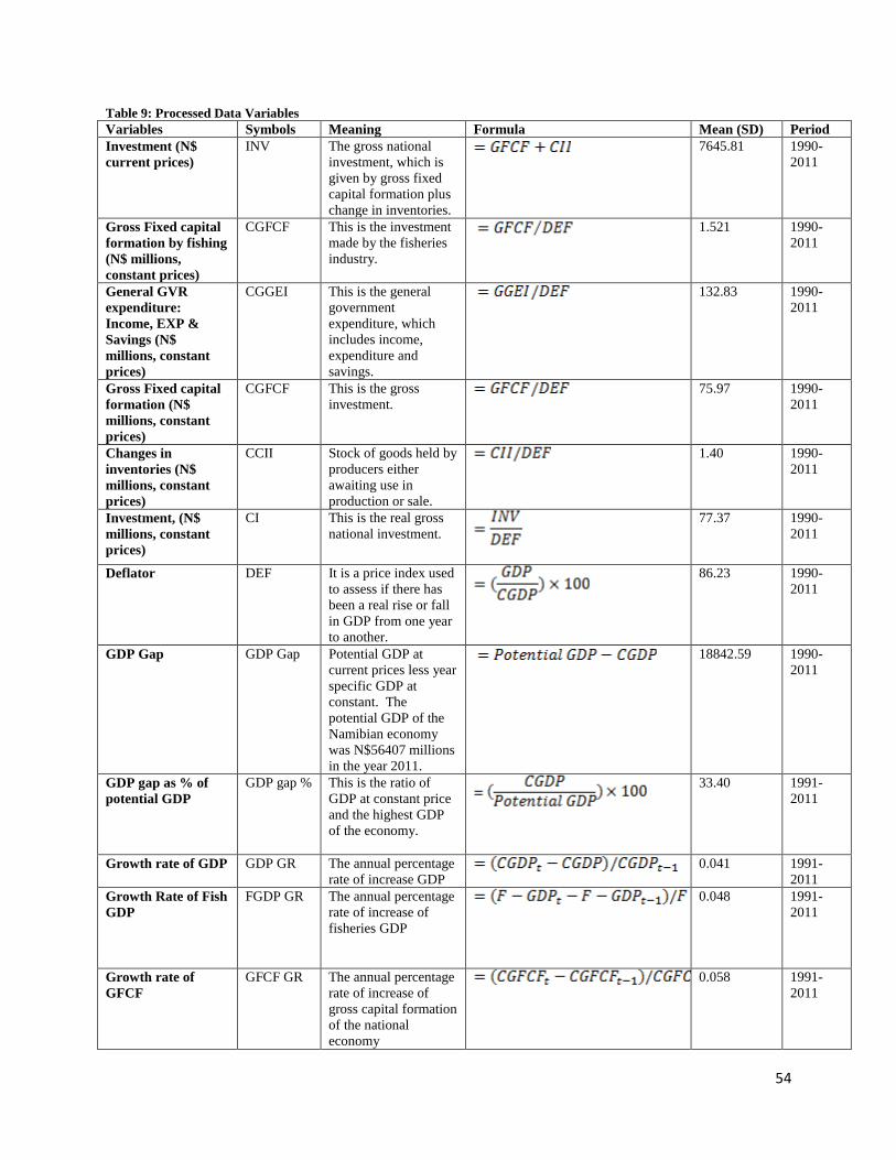
54

Table 9: Processed Data Variables

Variables Symbols Meaning Formula Mean (SD) Period

Investment (N$

current prices)

INV The gross national

investment, which is

given by gross fixed

capital formation plus

change in inventories.

7645.81 1990-

2011

Gross Fixed capital

formation by fishing

(N$ millions,

constant prices)

CGFCF This is the investment

made by the fisheries

industry.

1.521 1990-

2011

General GVR

expenditure:

Income, EXP &

Savings (N$

millions, constant

prices)

CGGEI This is the general

government

expenditure, which

includes income,

expenditure and

savings.

132.83 1990-

2011

Gross Fixed capital

formation (N$

millions, constant

prices)

CGFCF This is the gross

investment.

75.97 1990-

2011

Changes in

inventories (N$

millions, constant

prices)

CCII Stock of goods held by

producers either

awaiting use in

production or sale.

1.40 1990-

2011

Investment, (N$

millions, constant

prices)

CI This is the real gross

national investment.

77.37 1990-

2011

Deflator DEF It is a price index used

to assess if there has

been a real rise or fall

in GDP from one year

to another.

86.23 1990-

2011

GDP Gap GDP Gap Potential GDP at

current prices less year

specific GDP at

constant. The

potential GDP of the

Namibian economy

was N$56407 millions

in the year 2011.

18842.59 1990-

2011

GDP gap as % of

potential GDP

GDP gap % This is the ratio of

GDP at constant price

and the highest GDP

of the economy.

33.40 1991-

2011

Growth rate of GDP

GDP GR The annual percentage

rate of increase GDP

0.041 1991-

2011

Growth Rate of Fish

GDP

FGDP GR The annual percentage

rate of increase of

fisheries GDP

0.048 1991-

2011

Growth rate of

GFCF

GFCF GR The annual percentage

rate of increase of

gross capital formation

of the national

economy

0.058 1991-

2011

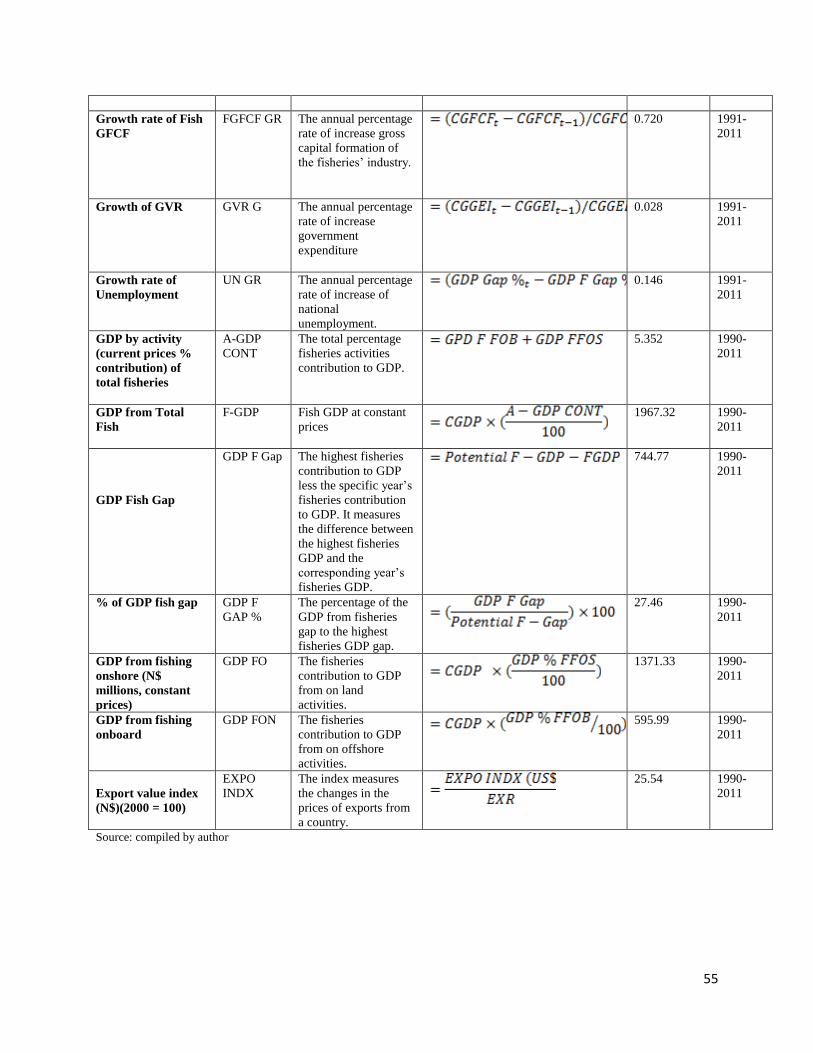
55

Growth rate of Fish

GFCF

FGFCF GR The annual percentage

rate of increase gross

capital formation of

the fisheries’ industry.

0.720 1991-

2011

Growth of GVR

GVR G The annual percentage

rate of increase

government

expenditure

0.028 1991-

2011

Growth rate of

Unemployment

UN GR The annual percentage

rate of increase of

national

unemployment.

0.146 1991-

2011

GDP by activity

(current prices %

contribution) of

total fisheries

A-GDP

CONT

The total percentage

fisheries activities

contribution to GDP.

5.352 1990-

2011

GDP from Total

Fish

F-GDP Fish GDP at constant

prices

1967.32 1990-

2011

GDP Fish Gap

GDP F Gap The highest fisheries

contribution to GDP

less the specific year’s

fisheries contribution

to GDP. It measures

the difference between

the highest fisheries

GDP and the

corresponding year’s

fisheries GDP.

744.77 1990-

2011

% of GDP fish gap

GDP F

GAP %

The percentage of the

GDP from fisheries

gap to the highest

fisheries GDP gap.

27.46 1990-

2011

GDP from fishing

onshore (N$

millions, constant

prices)

GDP FO The fisheries

contribution to GDP

from on land

activities.

1371.33 1990-

2011

GDP from fishing

onboard

GDP FON The fisheries

contribution to GDP

from on offshore

activities.

595.99 1990-

2011

Export value index

(N$)(2000 = 100)

EXPO

INDX

The index measures

the changes in the

prices of exports from

a country.

25.54 1990-

2011

Source: compiled by author

56

Table 10: Correlation matrix of the dependent and independent variables used in the basic

GDP growth rate estimation

GDP GR LAGlnCGDP GFCF GR GVR G FGDP GR UN GR T

Pearson Correlation

GDP GR 1.000 .017 .159 .176 -.148 -.377 .074

LAGlnCGDP .017 1.000 -.005 .413 -.289 -.602 .989

GFCF GR .159 -.005 1.000 .128 .195 -.022 -.020

GVR G .176 .413 .128 1.000 .145 -.295 .403

FGDP GR -.148 -.289 .195 .145 1.000 .080 -.321

UN GR -.377 -.602 -.022 -.295 .080 1.000 -.602

T .074 .989 -.020 .403 -.321 -.602 1.000

Sig. (1-tailed)

GDP GR . .472 .246 .222 .261 .046 .375

LAGlnCGDP .472 . .492 .031 .102 .002 .000

GFCF GR .246 .492 . .290 .198 .463 .466

GVR G .222 .031 .290 . .266 .097 .035

FGDP GR .261 .102 .198 .266 . .366 .078

UN GR .046 .002 .463 .097 .366 . .002

T .375 .000 .466 .035 .078 .002 .

N

GDP GR 21 21 21 21 21 21 21

LAGlnCGDP 21 21 21 21 21 21 21

GFCF GR 21 21 21 21 21 21 21

GVR G 21 21 21 21 21 21 21

FGDP GR 21 21 21 21 21 21 21

UN GR 21 21 21 21 21 21 21

T 21 21 21 21 21 21 21

Table 11: Summary statistics of the dependent and independent variables used in the basic

GDP growth

N Range Minimum Maximum Mean Std. Deviation Variance

Statistic Statistic Statistic Statistic Statistic Std. Error Statistic Statistic

GDP GR 22 .138 -.016 .123 .04377 .006646 .031170 .001

LAGlnCGDP 22 .85 10.09 10.94 10.5007 .05585 .26196 .069

GFCF GR 22 .572 -.190 .383 .04695 .032885 .154245 .024

GVR G 22 .479 -.314 .165 .02931 .020755 .097347 .009

FGDP GR 22 .706 -.242 .464 .04655 .036433 .170885 .029

UN GR 22 1.104 -1.000 .104 -.14295 .050237 .235632 .056

T 22 21 1 22 11.50 1.384 6.494 42.167

Valid N (listwise) 21

Table 12: ANOVA basic GDP growth Model Sum of Squares df Mean Square F Sig.

1

Regression .008 6 .001 1.866 .158

Residual .011 14 .001

Total .019 20

Dependent Variable: GDP GR Predictors: (Constant), T, GFCF GR, FGDP GR, GVR G, UN GR, LAGlnCGDP

57

Table 13: Basic GDP growth summary

Model R R Square Adjusted R

Square

Std. Error of

the Estimate

Durbin-

Watson

1 .667 .444 .206 .027390 1.534 Predictors: (Constant), T, GFCF GR, FGDP GR, GVR G, UN GR, LAGlnCGDP

Dependent Variable: GDP GR

Table 14: Summary statistics of the dependent and independent variables used in the other

basic GDP growth

N Range Minimum Maximum Mean Std. Deviation Variance

Statistic Statistic Statistic Statistic Statistic Std. Error Statistic Statistic

GDP GR 22 .138 -.016 .123 .04377 .006646 .031170 .001

LAGlnCGDP 22 .85 10.09 10.94 10.5007 .05585 .26196 .069

GFCF GR 22 .572 -.190 .383 .04695 .032885 .154245 .024

GVR G 22 .479 -.314 .165 .02931 .020755 .097347 .009

UN GR 22 1.104 -1.000 .104 -.14295 .050237 .235632 .056

T 22 21 1 22 11.50 1.384 6.494 42.167

Valid N (listwise) 21

Table 15: ANOVA, other basic GDP growth

Model Sum of Squares df Mean Square F Sig.

1

Regression .008 5 .002 2.033 .132

Residual .011 15 .001

Total .019 20

Dependent Variable: GDP GR

Predictors: (Constant), T, GFCF GR, GVR G, UN GR, LAGlnCGDP

Table16: Other basic GDP growth Model Summary

Model R R Square Adjusted R Square Std. Error of the

Estimate

Durbin-Watson

1 .636 .404 .205 .027407 1.481

Predictors: (Constant), T, GFCF GR, GVR G, UN GR, LAGlnCGDP

Dependent Variable: GDP GR

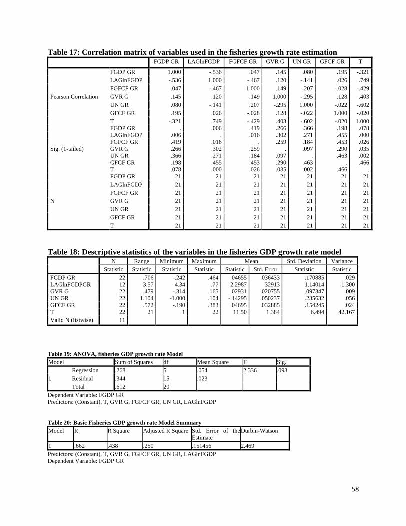
58

Table 17: Correlation matrix of variables used in the fisheries growth rate estimation

FGDP GR LAGlnFGDP FGFCF GR GVR G UN GR GFCF GR T

Pearson Correlation

FGDP GR 1.000 -.536 .047 .145 .080 .195 -.321

LAGlnFGDP -.536 1.000 -.467 .120 -.141 .026 .749

FGFCF GR .047 -.467 1.000 .149 .207 -.028 -.429

GVR G .145 .120 .149 1.000 -.295 .128 .403

UN GR .080 -.141 .207 -.295 1.000 -.022 -.602

GFCF GR .195 .026 -.028 .128 -.022 1.000 -.020

T -.321 .749 -.429 .403 -.602 -.020 1.000

Sig. (1-tailed)

FGDP GR . .006 .419 .266 .366 .198 .078

LAGlnFGDP .006 . .016 .302 .271 .455 .000

FGFCF GR .419 .016 . .259 .184 .453 .026

GVR G .266 .302 .259 . .097 .290 .035

UN GR .366 .271 .184 .097 . .463 .002

GFCF GR .198 .455 .453 .290 .463 . .466

T .078 .000 .026 .035 .002 .466 .

N

FGDP GR 21 21 21 21 21 21 21

LAGlnFGDP 21 21 21 21 21 21 21

FGFCF GR 21 21 21 21 21 21 21

GVR G 21 21 21 21 21 21 21

UN GR 21 21 21 21 21 21 21

GFCF GR 21 21 21 21 21 21 21

T 21 21 21 21 21 21 21

Table 18: Descriptive statistics of the variables in the fisheries GDP growth rate model

N Range Minimum Maximum Mean Std. Deviation Variance

Statistic Statistic Statistic Statistic Statistic Std. Error Statistic Statistic

FGDP GR 22 .706 -.242 .464 .04655 .036433 .170885 .029

LAGlnFGDPGR 12 3.57 -4.34 -.77 -2.2987 .32913 1.14014 1.300

GVR G 22 .479 -.314 .165 .02931 .020755 .097347 .009

UN GR 22 1.104 -1.000 .104 -.14295 .050237 .235632 .056

GFCF GR 22 .572 -.190 .383 .04695 .032885 .154245 .024

T 22 21 1 22 11.50 1.384 6.494 42.167

Valid N (listwise) 11

Table 19: ANOVA, fisheries GDP growth rate Model

Model Sum of Squares df Mean Square F Sig.

1

Regression .268 5 .054 2.336 .093

Residual .344 15 .023

Total .612 20

Dependent Variable: FGDP GR

Predictors: (Constant), T, GVR G, FGFCF GR, UN GR, LAGlnFGDP

Table 20: Basic Fisheries GDP growth rate Model Summary

Model R R Square Adjusted R Square Std. Error of the

Estimate

Durbin-Watson

1 .662 .438 .250 .151456 2.469

Predictors: (Constant), T, GVR G, FGFCF GR, UN GR, LAGlnFGDP

Dependent Variable: FGDP GR

59

Table 21: Descriptive statistics of the variables in the other basic fisheries GDP growth rate

model

N Range Minimum Maximum Mean Std. Deviation Variance

Statistic Statistic Statistic Statistic Statistic Std. Error Statistic Statistic

FGDP GR 22 .706 -.242 .464 .04655 .036433 .170885 .029

LAGlnFGDP 22 1.00 6.90 7.91 7.5503 .05986 .28075 .079

FGFCF GR 22 8.164 -.862 7.302 1.01922 .523904 2.457327 6.038

GVR G 22 .479 -.314 .165 .02931 .020755 .097347 .009

UN GR 22 1.104 -1.000 .104 -.14295 .050237 .235632 .056

GFCF GR 22 .572 -.190 .383 .04695 .032885 .154245 .024

T 22 21 1 22 11.50 1.384 6.494 42.167

Valid N (listwise) 21

Table 22: ANOVA other basic fisheries GDP growth

Model Sum of Squares df Mean Square F Sig.

1

Regression .288 6 .048 2.073 .122

Residual .324 14 .023

Total .612 20

Dependent Variable: FGDP GR

Predictors: (Constant), T, GFCF GR, GVR G, FGFCF GR, UN GR, LAGlnFGDP

Table 23: Other basic fisheries GDP growth summary

Model R R Square Adjusted R Square Std. Error of the

Estimate

Durbin-Watson

1 .686 .471 .244 .152146 2.482

Predictors: (Constant), T, GFCF GR, GVR G, FGFCF GR, UN GR, LAGlnFGDP

Dependent Variable: FGDP GR

HYPOTHESES testing regression output tables

Table 24: GDP growth vs. Initial GDP

Model Unstandardized Coefficients Standardized

Coefficients

t Sig.

B Std. Error Beta

1

(Constant) 3.310 1.833 1.806 .088

LAGlnCGDP -.327 .183 -2.648 -1.786 .091

T .013 .007 2.694 1.817 .086

Dependent Variable: GDP GR

Table 25: GDP growth vs. Initial GDP descriptive statistics

Mean Std. Deviation N

GDP GR .04377 .031170 22

LAGlnCGDP 10.5007 .26196 22

T 11.50 6.494 22

60

Table 26: GDP growth vs. Initial GDP correlations

GDP GR LAGlnCGDP T

GDP GR

Pearson Correlation 1 .017 -.032

Sig. (2-tailed) .943 .889

N 22 21 22

LAGlnCGDP

Pearson Correlation .017 1 .989**

Sig. (2-tailed) .943 .000

N 21 22 21

T

Pearson Correlation -.032 .989** 1

Sig. (2-tailed) .889 .000 N 22 21 22

**. Correlation is significant at the 0.01 level (2-tailed).

Table 27: GDP growth vs. Initial GDP Model Summary

Model R R Square Adjusted R Square Std. Error of the

Estimate

Durbin-Watson

1 .022 .000 -.058 .032284 2.131

Predictors: (Constant), LAGlnGDPGR

Dependent Variable: GDP GR

Table 28: GDP growth vs. Initial GDP ANOVA

Model Sum of Squares df Mean Square F Sig.

1

Regression .000 1 .000 .008 .929

Residual .018 17 .001

Total .018 18 Dependent Variable: GDP GR

Predictors: (Constant), LAGlnGDPGR

Table 29: GDP growth vs. Initial GDP descriptive statistics

Mean Std. Deviation N

GDP GR .04377 .031170 22

UN GR -.14295 .235632 22

T 11.50 6.494 22

Table 30: GDP growth vs. Initial GDP correlation

GDP GR UN GR T

Pearson Correlation

GDP GR 1.000 -.340 -.032

UN GR -.340 1.000 -.588

T -.032 -.588 1.000

Sig. (1-tailed)

GDP GR . .061 .444

UN GR .061 . .002

T .444 .002 .

N

GDP GR 22 22 22

UN GR 22 22 22

T 22 22 22

61

Table 31: GDP growth vs. Initial GDP model summary

Model R R Square Adjusted R Square Std. Error of the

Estimate

Durbin-Watson

1 .445 .198 .113 .029348 1.634

Predictors: (Constant), T, UN GR

Dependent Variable: GDP GR

Table 32: GDP growth vs. Initial GDP ANOVA

Model Sum of Squares df Mean Square F Sig.

1

Regression .004 2 .002 2.344 .123

Residual .016 19 .001

Total .020 21 Dependent Variable: GDP GR

Predictors: (Constant), T, UN GR

Table 33: GDP growth vs. Initial GDP coefficients

Model Unstandardized Coefficients Standardized

Coefficients

t Sig.

B Std. Error Beta

1

(Constant) .053 .013 3.951 .001

UN GR -.073 .034 -.549 -2.160 .044

T -.002 .001 -.354 -1.395 .179

Dependent Variable: GDP GR

Table 34: GDP growth vs. gross fixed capital formation

descriptive statistics

Mean Std. Deviation N

GDP GR .04377 .031170 22

GFCF GR .04695 .154245 22

T 11.50 6.494 22

Table 35: GDP growth vs. gross fixed capital formation correlations

GDP GR GFCF GR T

Pearson Correlation

GDP GR 1.000 .050 -.032

GFCF GR .050 1.000 .106

T -.032 .106 1.000

Sig. (1-tailed)

GDP GR . .412 .444

GFCF GR .412 . .319

T .444 .319 .

N

GDP GR 22 22 22

GFCF GR 22 22 22

T 22 22 22

Table 36: GDP growth vs. gross fixed capital formation correlations model summary

Model R R Square Adjusted R Square Std. Error of the

Estimate

Durbin-Watson

1 .063 .004 -.101 .032706 1.836

Predictors: (Constant), T, GFCF GR

Dependent Variable: GDP GR

62

Table 37: GDP growth vs. gross fixed capital formation correlations model summary ANOVA

Model Sum of Squares df Mean Square F Sig.

1

Regression .000 2 .000 .037 .963

Residual .020 19 .001

Total .020 21 Dependent Variable: GDP GR

Predictors: (Constant), T, GFCF GR

Table 38: GDP growth vs. gross fixed capital formation correlations coefficients

Model Unstandardized Coefficients Standardized

Coefficients

t Sig.

B Std. Error Beta

1

(Constant) .045 .014 3.134 .005

GFCF GR .011 .047 .054 .236 .816

T .000 .001 -.037 -.163 .872

Dependent Variable: GDP GR