M.H. Perrott © 2007 Filtering in Continuous and Discrete Time, Slide 1

Filtering inContinuous andDiscrete Time

• Lowpass, highpass, bandpass filtering • Filter response to cosine wave inputs• Discrete-Time Fourier Transform• Filtering based on difference equations

Copyright © 2007 by M.H. PerrottAll rights reserved.

M.H. Perrott © 2007 Filtering in Continuous and Discrete Time, Slide 2

0

X(f)

Voiceband

frequencies

f

RF transmission

frequencies

0

Y(f)

Voiceband

frequencies

f

RF reception

frequencies

RF

Transmitter

Voice

RF

Transmission

RF

Receiver

Voice

RF

Reception

Interferer

Motivation for Filtering

• Filtering is used to remove undesired signals outside of the frequency band of interest– Enables selection of a specific radio, TV, WLAN, cell

phone, cable TV channel …– Undesired channels are often called interferers

M.H. Perrott © 2007 Filtering in Continuous and Discrete Time, Slide 3

1

0f

fo

R(f)

-fo 2fo-2fo

2A

0f

fo

W(f)

-fo

A A

2fo-2fo

2A

0f

fo

H(f)

-fo 2fo-2fo

Lowpass Filter

• Only low frequency (i.e. baseband) portion remains

y(t) = 2cos(2πfot)

z(t) r(t)

Lowpass

Filterw(t)

H(f)

M.H. Perrott © 2007 Filtering in Continuous and Discrete Time, Slide 4

1

0f

fo

R(f)

-fo 2fo-2fo

0f

fo

W(f)

-fo

A A

2fo-2fo

2A

0f

fo

H(f)

-fo 2fo-2fo

A A

1

Highpass Filter

• Only high frequency (i.e. RF) portion remains

y(t) = 2cos(2πfot)

z(t) r(t)

Highpass

Filterw(t)

H(f)

M.H. Perrott © 2007 Filtering in Continuous and Discrete Time, Slide 5

1

0f

fo

R(f)

-fo 2fo-2fo

0f

fo

W(f)

-fo

A A

2fo-2fo

2A

0f

fo

H(f)

-fo 2fo-2fo

A A

1

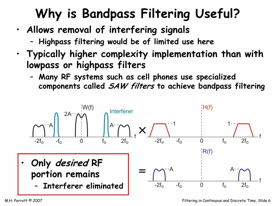
Bandpass Filter

• Only high frequency (i.e. RF) portion remains

y(t) = 2cos(2πfot)

z(t) r(t)

Bandpass

Filterw(t)

H(f)

M.H. Perrott © 2007 Filtering in Continuous and Discrete Time, Slide 6

1

0f

fo

R(f)

-fo 2fo-2fo

0f

fo

W(f)

-fo

A A

2fo-2fo

2A

0f

fo

H(f)

-fo 2fo-2fo

A A

1

Interferer

• Only desired RF portion remains– Interferer eliminated

Why is Bandpass Filtering Useful?• Allows removal of interfering signals

– Highpass filtering would be of limited use here• Typically higher complexity implementation than with

lowpass or highpass filters– Many RF systems such as cell phones use specialized

components called SAW filters to achieve bandpass filtering

M.H. Perrott © 2007 Filtering in Continuous and Discrete Time, Slide 7

ffc

K

-fc

K2

1

0f

fc

K

-fc 0

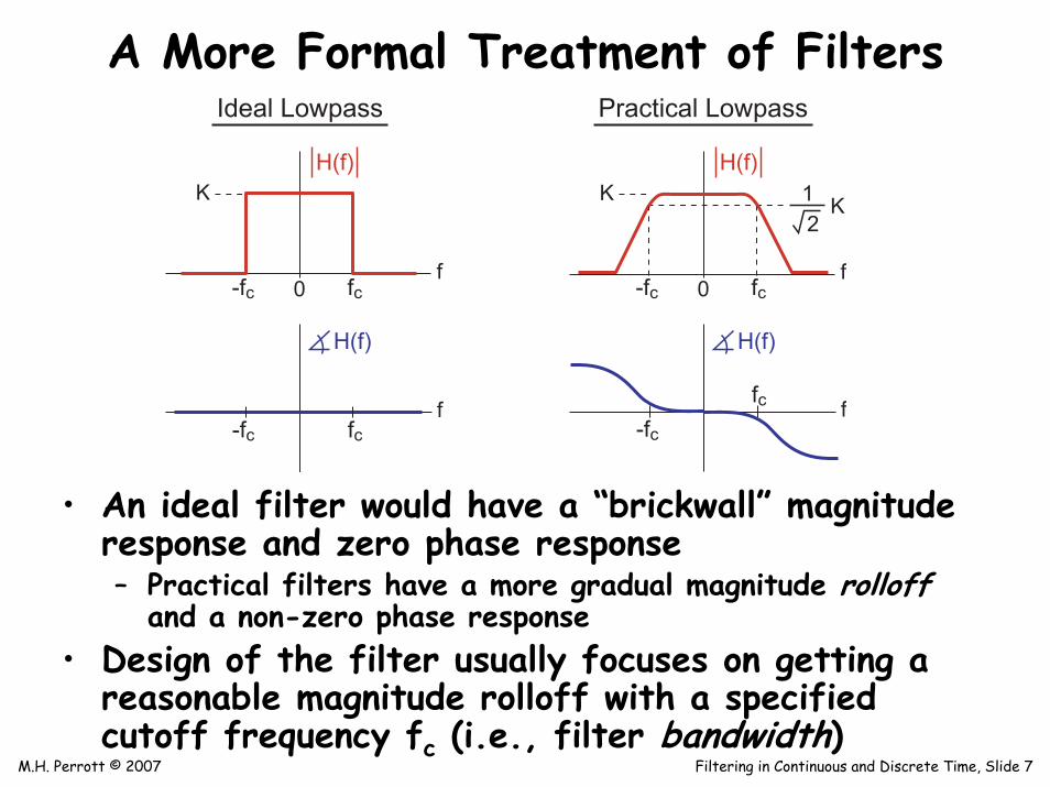
Ideal Lowpass Practical Lowpass

H(f)

H(f)

ffc-fc

H(f)

ffc

-fc

H(f)

A More Formal Treatment of Filters

• An ideal filter would have a “brickwall” magnitude response and zero phase response– Practical filters have a more gradual magnitude rolloff

and a non-zero phase response• Design of the filter usually focuses on getting a

reasonable magnitude rolloff with a specified cutoff frequency fc (i.e., filter bandwidth)

M.H. Perrott © 2007 Filtering in Continuous and Discrete Time, Slide 8

ffo

K

-fo 0

H(f)

f

H(f)

0

1

ffo

X(f)

1

-fo

fo-fo

Lowpass Filter: H(f)

0f

fo

Y(f)

-fo

H(fo)H(fo)

ej

H(-fo)H(-fo)

ej

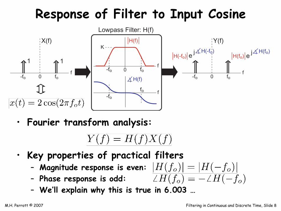
Response of Filter to Input Cosine

• Fourier transform analysis:

• Key properties of practical filters– Magnitude response is even:– Phase response is odd:– We’ll explain why this is true in 6.003 …

M.H. Perrott © 2007 Filtering in Continuous and Discrete Time, Slide 9

Compute Fourier Transform

• Fourier transform of output:

Define:

ffo

K

-fo 0

H(f)

f

H(f)

0

1

ffo

X(f)

1

-fo

fo-fo

Lowpass Filter: H(f)

0f

fo

Y(f)

-fo

H(fo)H(fo)

ej

H(-fo)H(-fo)

ej

M.H. Perrott © 2007 Filtering in Continuous and Discrete Time, Slide 10

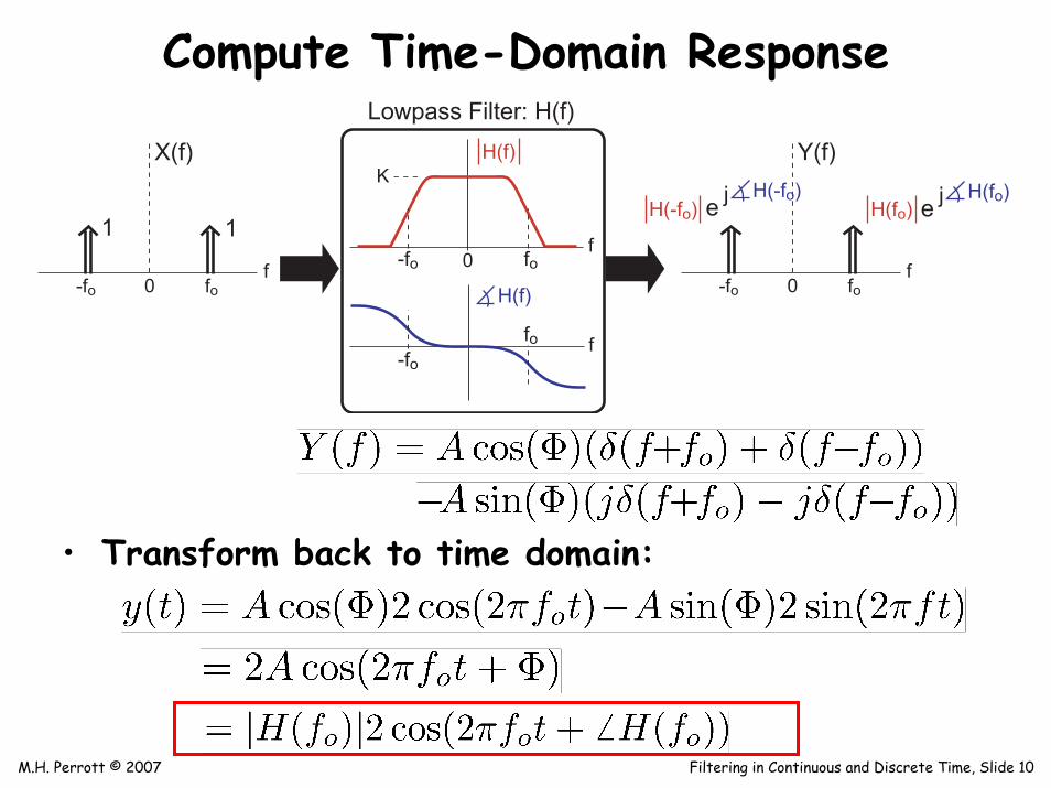
Compute Time-Domain Response

• Transform back to time domain:

ffo

K

-fo 0

H(f)

f

H(f)

0

1

ffo

X(f)

1

-fo

fo-fo

Lowpass Filter: H(f)

0f

fo

Y(f)

-fo

H(fo)H(fo)

ej

H(-fo)H(-fo)

ej

M.H. Perrott © 2007 Filtering in Continuous and Discrete Time, Slide 11

ffo

K

-fo 0

H(f)

f

H(f)

0

1

ffo

X(f)

1

-fo

fo-fo

Lowpass Filter: H(f)

0f

fo

Y(f)

-fo

H(fo)H(fo)

ej

H(-fo)H(-fo)

ej

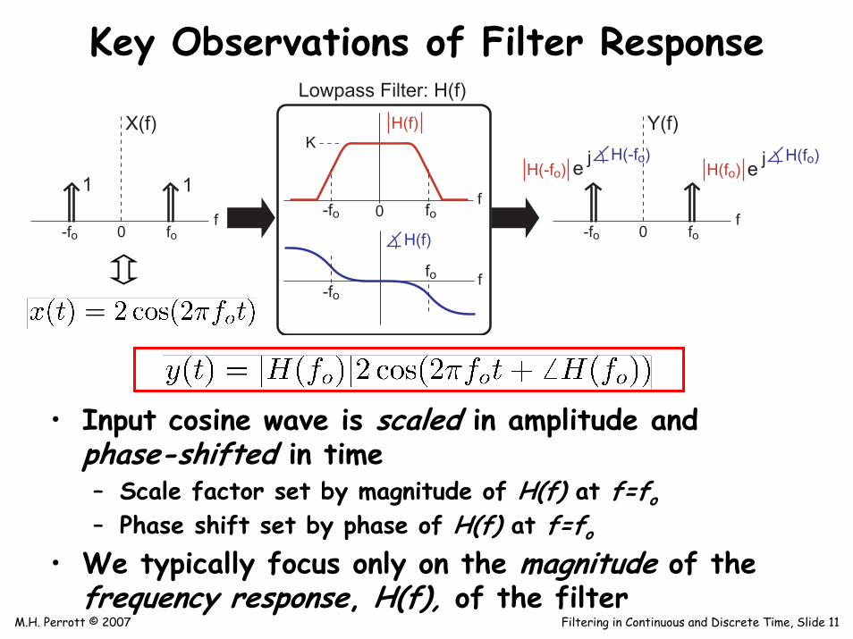
Key Observations of Filter Response

• Input cosine wave is scaled in amplitude and phase-shifted in time– Scale factor set by magnitude of H(f) at f=fo– Phase shift set by phase of H(f) at f=fo

• We typically focus only on the magnitude of the frequency response, H(f), of the filter

M.H. Perrott © 2007 Filtering in Continuous and Discrete Time, Slide 12

Designing and Using Filters Within Matlab

• Our lab exercises will have you design and use filters in Matlab– Matlab will interface to the USRP board in order to

receive “real world” signals from the antenna• Matlab framework is based on discrete-time

sequences (which are indexed on integer values)– Correspond to samples of corresponding real world signals

(which are continuous-time in nature)

n

x[n]

1

x(t)

t

Real World Matlab

We need another Fourier analysis tool

M.H. Perrott © 2007 Filtering in Continuous and Discrete Time, Slide 13

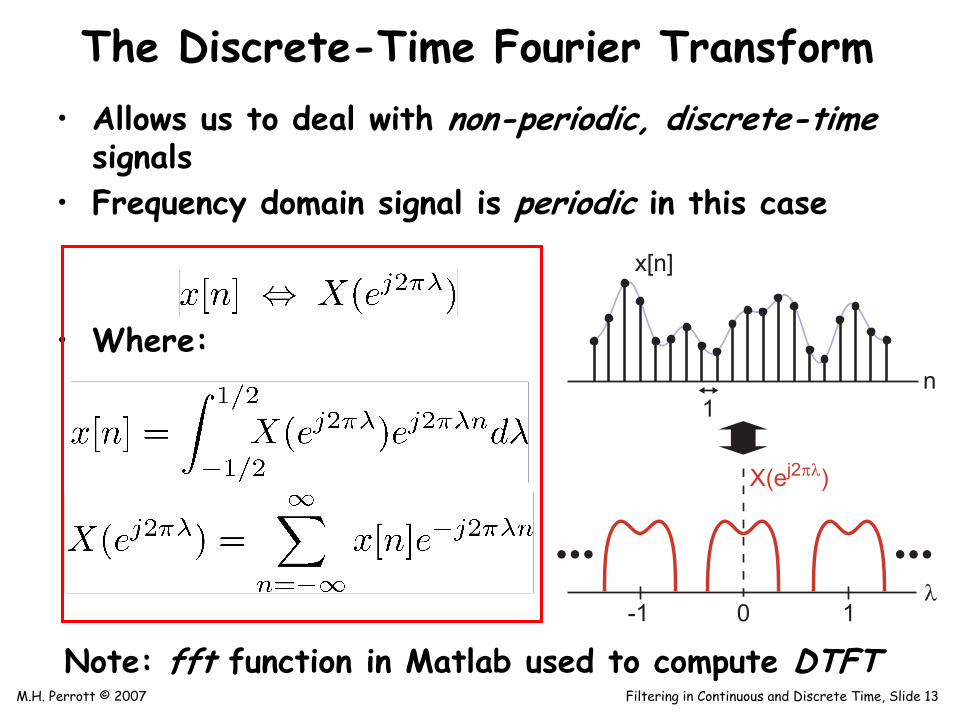
The Discrete-Time Fourier Transform• Allows us to deal with non-periodic, discrete-time

signals• Frequency domain signal is periodic in this case

• Where:n

x[n]

1

0λ

X(ej2πλ)

1-1

Note: fft function in Matlab used to compute DTFT

M.H. Perrott © 2007 Filtering in Continuous and Discrete Time, Slide 14

n

x[n]

1

0λ

X(ej2πλ)

1-1

t

x(t)

T

0f

X(f)

1/T-1/T

Matlab Sequence Samples of Real World Signal

Relating to Samples of `Real World’ Signals

• Samples of a continuous-time signal with sample period T leads to frequency domain signal with period 1/T– We simply scale frequency axis of fft in Matlab

• We will say much more about sampling later …

M.H. Perrott © 2007 Filtering in Continuous and Discrete Time, Slide 15

Filters Within Matlab

• Implemented as difference equations– Current output, y[n], depends on weighted values of

previous output samples and current and previous input samples, x[n]

• Group a and b coefficients as vectors:

• Execute filter using the filter command:

Discrete-Time

Filterx[n]

H(ej2πλ)

n

x[n]

1

y[n]

n

1

y[n]

M.H. Perrott © 2007 Filtering in Continuous and Discrete Time, Slide 16

Impact of Delay on DTFT

• Consider a signal that is a delayed version of another signal:

• Compute DTFT of y[n]

M.H. Perrott © 2007 Filtering in Continuous and Discrete Time, Slide 17

Compute Filter Response using DTFT

• Make use of the time shift property:

• Filter response is simply ratio of output over input:

M.H. Perrott © 2007 Filtering in Continuous and Discrete Time, Slide 18

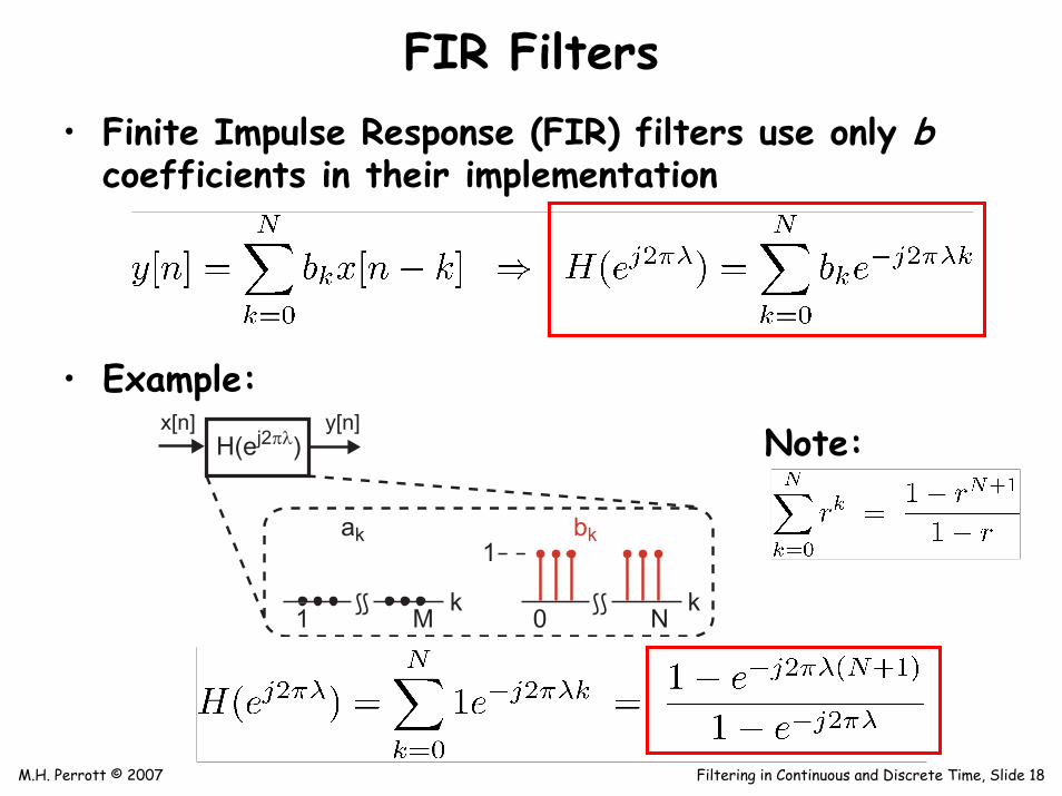
FIR Filters• Finite Impulse Response (FIR) filters use only b

coefficients in their implementation

• Example:x[n]

H(ej2πλ)y[n]

k

bk

Nk

ak

M1

1

0

Note:

M.H. Perrott © 2007 Filtering in Continuous and Discrete Time, Slide 19

Filter Order for FIR Filters

• Consider two different values for N

• Higher N leads to steeper filter response– We refer to N as the order of the filter

λ

H(ej2πλ)

0 1-1

8

λ

H(ej2πλ)

0 1-1

4

N=3 N=7

x[n]H(ej2πλ)

y[n]

k

bk

Nk

ak

M1

1

0

M.H. Perrott © 2007 Filtering in Continuous and Discrete Time, Slide 20

FIR Filter Design in Matlab

• Lowpass, highpass, and bandpass filters can be realized by appropriately scaling the relative value of the b coefficients– Higher order (i.e., higher N) leads to steeper responses

• Perform FIR filter design using fir1 command• Frequency response observed with freqz command

x[n]H(ej2πλ)

y[n]

k

bk

Nk

ak

M1

K

0

See Prelab portion of Lab 3 for details …

M.H. Perrott © 2007 Filtering in Continuous and Discrete Time, Slide 21

Summary• Filters can generally be classified according to

– Lowpass, highpass, bandpass operation– Bandwidth and order of filter

• Given a cosine input to a filter, output is:– Scaled in amplitude by magnitude of filter frequency response– Shifted in phase by phase of filter frequency response

• Matlab operates on discrete-time signals– Use DTFT for analytical analysis– Use commands such as fir1, freqz, and filter for design and

implementation of FIR filters

• Next lecture: introduce I/Q modulation and further discuss continuous-time filtering