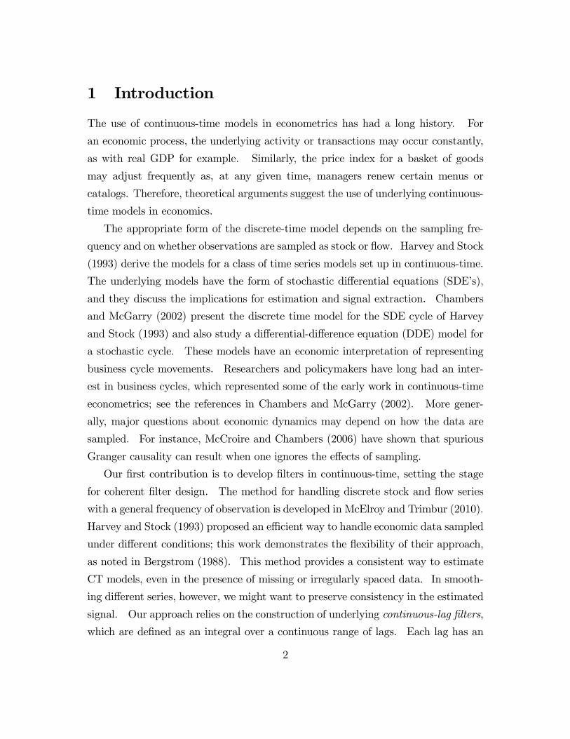
Continuous-Time Signal Extraction: Filter

Design for Economic Time Series

Tucker S. McElroy, U.S. Census Bureau, Washington DC

Thomas M. Trimbur∗, Federal Reserve Board, Washington DC

April, 2010

Abstract

This paper sets out the theoretical foundations for continuous-time signal ex-

traction in econometrics. Continuous-time modeling gives an effective strategy

for treating stock and flow data, irregularly spaced data, and changing fre-

quency of observation. We rigorously derive the optimal continuous-lag filter

when the signal component is nonstationary, and provide several illustrations,

including a new class of continuous-lag Butterworth filters for trend and cycle

estimation.

Keywords: Band Pass Filters, Continuous TimeModels, Cycles, Hodrick-Prescott

Filter, Turning points

JEL classification: C22, E32.

Disclaimer: This report is released to inform interested parties of research and

to encourage discussion. The views expressed on economic and statistical issues are

those of the authors and not necessarily those of the U.S. Census Bureau or of the

Federal Reserve Board.

∗Corresponding author. Address: Division of Research and Statistics; 20th and C Street, NW;

Federal Reserve Board; Washington, DC 20551. Email: Thomas.M.Trimbur@frb.gov.

1

1 Introduction

The use of continuous-time models in econometrics has had a long history. For

an economic process, the underlying activity or transactions may occur constantly,

as with real GDP for example. Similarly, the price index for a basket of goods

may adjust frequently as, at any given time, managers renew certain menus or

catalogs. Therefore, theoretical arguments suggest the use of underlying continuous-

time models in economics.

The appropriate form of the discrete-time model depends on the sampling fre-

quency and on whether observations are sampled as stock or flow. Harvey and Stock

(1993) derive the models for a class of time series models set up in continuous-time.

The underlying models have the form of stochastic differential equations (SDE’s),

and they discuss the implications for estimation and signal extraction. Chambers

and McGarry (2002) present the discrete time model for the SDE cycle of Harvey

and Stock (1993) and also study a differential-difference equation (DDE) model for

a stochastic cycle. These models have an economic interpretation of representing

business cycle movements. Researchers and policymakers have long had an inter-

est in business cycles, which represented some of the early work in continuous-time

econometrics; see the references in Chambers and McGarry (2002). More gener-

ally, major questions about economic dynamics may depend on how the data are

sampled. For instance, McCroire and Chambers (2006) have shown that spurious

Granger causality can result when one ignores the effects of sampling.

Our first contribution is to develop filters in continuous-time, setting the stage

for coherent filter design. The method for handling discrete stock and flow series

with a general frequency of observation is developed in McElroy and Trimbur (2010).

Harvey and Stock (1993) proposed an efficient way to handle economic data sampled

under different conditions; this work demonstrates the flexibility of their approach,

as noted in Bergstrom (1988). This method provides a consistent way to estimate

CT models, even in the presence of missing or irregularly spaced data. In smooth-

ing different series, however, we might want to preserve consistency in the estimated

signal. Our approach relies on the construction of underlying continuous-lag filters,

which are defined as an integral over a continuous range of lags. Each lag has an

2

associated weight density. The theory, tracing back to Hannan (1970) and Priestley

(1973), involves a general formulation including the Continuous-Time Autoregres-

sive Integrated Moving Average (CARIMA) processes of Brockwell and Marquardt

(2005). We also treat the case of a white noise irregular, which is frequently used

in standard models in continuous-time econometrics. Since continuous-time white

noise is heuristically the first derivative of Brownian motion (which is nowhere dif-

ferential), this requires a careful mathematical treatment to ensure that the signal

extraction problem is well-defined.

As a second contribution, we give a rigorous proof of optimality for the filters of

interest in econometrics. In particular, we prove the signal extraction formula for

nonstationary continuous-time models. Bell (1984) set out the foundation for signal

extraction for nonstationary series in discrete-time; in this paper, we generalize

his argument to continuous-time. As Whittle’s (1983) results only covered the

stationary case, the proof in the case of trend nonstationarity, given in Section 3,

fills an important gap in the literature.

Third, we present a number of filters for econometric analysis, including ones

geared toward detecting turning points and band-pass filters designed to extract

the cyclical component. The design of continuous-lag filters, illustrated in Section

4, naturally leads to the construction of a coherent set of discrete filters. This

discretization of the filter occurs directly, without the need for deducing the discrete-

time model corresponding to each particular frequency. We show an application to

US CPI inflation in Section 5.

The rest of the paper is organized as follows. Section 2 reviews continuous-time

filtering, based on material from Priestley (1981), Hannan (1970), and Koopmans

(1974). Section 3 sets out the signal extraction framework. In section 4, examples are

given for economic series; an extension of the standard HP filter is derived from the

smooth trend model, and a general class of band-pass filters is presented. Extensions

to methodology are then described, specifically, the conversion of continuous-lag fil-

ters to estimate growth rates and other characteristics of an underlying component.

Section 5 discusses the application of the method to real series, and Section 6 con-

cludes. Proofs are given in the Appendix.

3

2 Continuous-Time Processes and Filters

This section sets out the theoretical framework for the analysis of continuous-time

signal processing and filtering. The goal is to set the stage for the development

of coherent discrete filters in a wide range of applications. Much of the treatment

follows Hannan (1970); also see Priestley (1981) and Koopmans (1974). We start

by setting up a fundamental signal extraction problem and by investigating the

properties of the optimal continuous-lag filters This part of the frequency and time

domain analysis is done independently of sampling type and interval and so may be

seen as fundamental to the dynamics of the problem.

Let () for ∈ R, the set of real numbers, denote a real-valued time series thatis measurable and square-integrable at each time. The process is weakly stationary

by definition if it has constant mean — set to zero for simplicity — and autocovariance

function given by

() = E[()(+ )] ∈ R (1)

Note that the autocovariances are defined for the continuous range of lags . Thus

if () is a Gaussian process, completely describes the dynamics of the stochastic

process. A convenient representation for stationary continuous-time processes that

is analogous to moving averages in discrete time series is given by

() = ( ∗ )() =Z ∞

−∞()(− ) (2)

where (·) is square integrable on R, and () is continuous-time white noise (WN).In this case, () = ( ∗ −)(), where −() = (−). If () is Gaussian,then () = (), the derivative of a standard Wiener process. Though ()

is nowhere differentiable, () can be defined using the theory of Generalized Ran-

dom Processes, as in Hannan (1970, p. 23). It is convenient to work with models

expressed in terms of the disturbance (), because this makes it easy to see the

connection with discrete models based on white noise disturbances.

As an example, Brockwell’s (2001) Continuous-time Autoregressive Moving Av-

erage (CARMA) models can be written as

()() = ()()4

where () is a polynomial of order , and () is a polynomial of order , and

is the derivative operator. The condition for stationarity is analogous to the one

for a discrete AR polynomial: the roots of the equation () = 0 must all have

strictly negative real part. It can be shown (Brockwell and Marquardt, 2005) that

() following such a stationary CARMA model can be re-expressed in the form (2),

for an appropriate .

Next, we define the continuous-time lag operator via the equation

() = (− ) (3)

for any ∈ R and for all times ∈ R. We denote the identity element 0 by 1,just as in discrete time. Then a Continuous-Lag Filter is an operator Ψ() with

associated weighting kernel (an integrable function) such that

Ψ() =

Z ∞

−∞() (4)

The effect of the filter on a process () is

Ψ()() =

Z ∞

−∞() (− ) = ( ∗ )() (5)

The requirement of integrability for the function () is a mild condition that is

sufficient for many problems. However, when the input process is nonintegrable over

, an integrable () may become inadmissible as a kernel, i.e., it may fail to give

a well-defined process as output. In such a case, we may need to assume that is

differentiable to a specified order, with integrable or square integrable derivatives.

This development parallels the discussion in Priestley (1981), where the filter is

written as

L[]() =Z ∞

−∞()−

with L[] denoting the Laplace transform of . As will be discussed below, we can

make the identification = − log, which effectively maps Priestley’s formulationinto (4).

5

2.1 Continuous-lag filters in the Frequency Domain

In analogy with the discrete-time case, the frequency response function is obtained

by replacing by the argument −:

Ψ(−) =Z ∞

−∞() − ∈ R (6)

Denoting the continuous-time Fourier Transform by F [·], equation (6) can be writtenas Ψ(−) = F []().

Example 1 Consider a Gaussian kernel () = 1√2−

2

2 In this example, the

inclusion of the normalizing constant means that the function integrates to one;

since applying the filter tends to preserve the level of the process, it could be used

as a simple trend estimator. The frequency response has the same form as the

weighting kernel and is given by F []() = −2

2 .

The power spectrum of a continuous time process () is the Fourier Transform

of its autocovariance function :

() = F []() ∈ R (7)

The gain function of a filterΨ() is the magnitude of the frequency response, namely

() = |F []()| ∈ R (8)

As in discrete time series signal processing, passing an input (stationary) process

through the filter Ψ() results in an output process with spectrum multiplied by the

squared gain; so the gain function gives information about how contributions to the

variance at various frequencies are attenuated or accentuated by the filter. Note that

in contrast to the discrete case where the domain is restricted to the interval [− ]the functions in (7) and (8) are defined over the entire real line. Given a candidate

gain function () taking the inverse Fourier Transform in continuous-time yields

the associated weighting kernel:

F−1[]() = 1

2

Z ∞

−∞() ∈ R (9)

This expression is well-defined for any integrable (). Integrability is a mild con-

dition satisfied by nearly all filters of practical interest.

6

Example 2 Weighting kernels that decay exponentially on either side of the ob-

servation point have often been applied in smoothing trends; this pattern arises

frequently in discrete model-based frameworks, e.g., Harvey and Trimbur (2003).

Similarly, in the continuous time setting, a simple example of a trend estimator is

the double exponential weighting pattern () = 12−||, ∈ R In this case, one can

show using integral calculus that Ψ() = 1(1 − (log)2), as a formal expression.The Fourier transform has the same form as a Cauchy probability density function,

namely F []() = 1(1 + 2). This means that the gain of the low-pass filter Ψ()

decays slowly as −→∞

2.2 The Derivative Filter and Nonstationary Processes

In (3), the extension of the lag operator to the continuous-time framework is

made explicit. In building models, we can treat as an algebraic quantity as in the

discrete-time framework. The extension of the differencing operator, ∆ = 1 − ,

used to define nonstationary models, is discussed in Hannan (1970, p. 55) and

Koopmans (1974).

To define the mean-square differentiation operator , consider the limit of mea-

suring the displacement of a continuous-time process, per unit of time, over an

arbitrarily small interval :

() = lim

→0()− (− )

= lim

→01−

() = (− log)()

The limits are interpreted to converge in mean square. Thus, we see that taking

the derivative has the same effect as applying the continuous lag filter − log.This holds for all mean-square differentiable processes (), implying = − log;note that Priestley (1981) derives the equivalent = exp{−} via Taylor seriesarguments. This operator will be our main building block for nonstationary

continuous-time processes. It will also be useful in thinking about rates of growth

and rates of rates of growth — the velocity and acceleration of a process, respec-

tively. We refer to − log as the derivative filter; taking powers yields higher orderderivative filters. For instance, (log)2 gives a measure of acceleration with respect

to time. We note that the frequency response of is (−).7

Standard discrete-time ARIMA processes are written as difference equations,

built on white noise disturbances. In analogy, continuous time processes can be

written as differential equations, built on an extension of white noise to continuous-

time. Thus a natural class of models is the Integrated Filtered Noise processes,

which are given by

() = Ψ()() (10)

for some integrable , and order of differential ≥ 0. This class will be denoted() ∼ (); it encompasses a wide variety of linear continuous-time models. As

an example, Brockwell and Marquardt (2005) define the class of Continuous-time

Autoregressive Integrated Moving Average (CARIMA) models as the solution to

()() = ()() (11)

Thus, applying the -fold derivative filter transforms () into a stationary CARMA

(p,q) process. The autoregressive order is the degree of the polynomial (),

and the moving average order is the degree of the polynomial (). The constraint

is necessary to ensure the process is well-defined; this ensures that the spectral

density of () is an integrable function. This gives the CARIMA(p,d,q) process.

The original process () is nonstationary and is said to be integrated of order

in the continuous-time sense. Now this can be put into an () form: starting

from (11), we can write (formally)

() = [()()] () (12)

Using the definition of, it follows that () ∼ () withΨ() = (− log)(− log).Deriving the kernel () requires an expression for the rational function in terms of

an integral over powers of , namely (− log)(− log) = R∞−∞ () . Using

the formulation of Priestley (1981), we see that models can be equiva-

lently expressed as models where the kernel ’s Laplace transform is a rational

function.

Example 3: Higher order stochastic cycles The study of business cycles

has remained of interest to researchers and policymakers for some time. Some of

8

the early work in continuous-time econometrics was geared toward this application;

Kalecki (1935) and James and Belz (1936). Recently, Chambers and McGarry

(2002) also used a model in the form of a differential-difference equation (DDE)

to describe business cycle movements. Here, we focus on the SDE form that has

convenient representations in the time and frequency domains. The class of higher

order cycles was introduced in Harvey and Trimbur (2003) for discrete models, and

we generalize the construction to continuous-time. These structural models have an

intuitive structure where the frequency of fluctuations center around a parameter .

We derive analytical expressions for the spectral density, giving a clear summary of

the cyclical properties of the model.

The class of continuous-time stochastic cycles are indexed by a positive integer

that denotes the order of the model. Denote the cyclical process by (), and let

∗() represent an auxiliary process used in the construction of the model. Define

ψ() = (() ∗())

0. An −th order stochastic cycle is given by

ψ() = Aψ()+

"−1()

0

# = 2 (13)

ψ1() = Aψ1()+

"()

0

# () ∼

¡02

¢where ψ() = (()

∗ ())

0 = 1 −1 represent additional auxiliary processes.The coefficient matrix in (13) is

A =

"log

− log

#

The parameter is called the damping factor; it satisfies 0 ≤ 1. The stochasticvariation in the cycle per unit time depends on the continuous-time variance para-

meter 2. The parameter controls the persistence of cyclical fluctuations, and

its specific role depends on . Generally, for higher orders, the model generates

smoother dynamics for the cycle.

Since the parameter corresponds roughly to a peak in the spectrum, it indi-

cates a central frequency of the cycle, and 2 is an average period of oscillation.

9

As is a frequency in continuous-time, it can be any positive real number, though

for macroeconomic data, business cycle theory will usually suggest a value in some

intermediate range.

To construct a Gaussian cyclical process, the increment () can be derived from

Brownian motion (), that is, () ∼ ().

In analyzing cyclical behavior, it is natural to consider the frequency domain

properties. To derive the spectra for various , start by rewriting (13) as a recursive

formula: " − log − − log

#"()

∗ ()

#=

"−1()

0

# = 1

with the initialization 0() = (). The solution is

(( − log )2 + 2)() = ( − log )()

so that the th order cycle has a CARMA(2n,n) form. The power spectrum is

() = 2

"2 + log2 ¡

log2 + (− )2¢ ¡log2 + (+ )

2¢#

(14)

One advantage of working with the cycle in continuous-time is the possibility of

analyzing turning points instantaneously. The expected incremental change in the

cycle for ≥ 2 is

() = (log )()+ ∗()+ −1() (15)

For = 1, this reduces to

1() = (log )1()+ ∗1() (16)

Based on the smoothness of estimated cycles, the higher order models are likely to

give more reliable indication of turning points.

Expression (16) is similar to the one in Harvey (1989, p. 487). There is, however,

a slight difference because the form in (13) is analogous to the ‘Butterworth form’

used in Harvey and Trimbur (2003). The alternative form in Harvey (1989) and

in Harvey and Stock (1985) is analogous to the ‘balanced form’ also considered in

10

Harvey and Trimbur (2003). The key advantage of the Butterworth form, as used

here, is its convenience for the analysis of spectra and gain functions.

We have shown that the class of models in (13) are equivalent to CARMA

processes whose parameters satisfy the conditions needed for periodic behavior. As

an alternative, an openly specified model can be used to describe a general pattern

of serial correlation; thus, a CAR(1) could be used to capture first-order autocor-

relation in the noise component, for instance, due to temporary effects of weather.

When there is clear indication of cyclical dynamics, however, the models in (13) give

a more direct analysis that is easier to interpret.

The properties of a class of stochastic cycles1 are set out in Trimbur (2006) for

the discrete-time case. The properties of the continuous-time models give a similar

flexibility in describing periodic behavior.

0.5 1 1.5 2 2.5Λ

0.2

0.4

0.6

0.8

1

1.2

1.4

1.6

1.8

F�Λ�

n � 1

n � 2

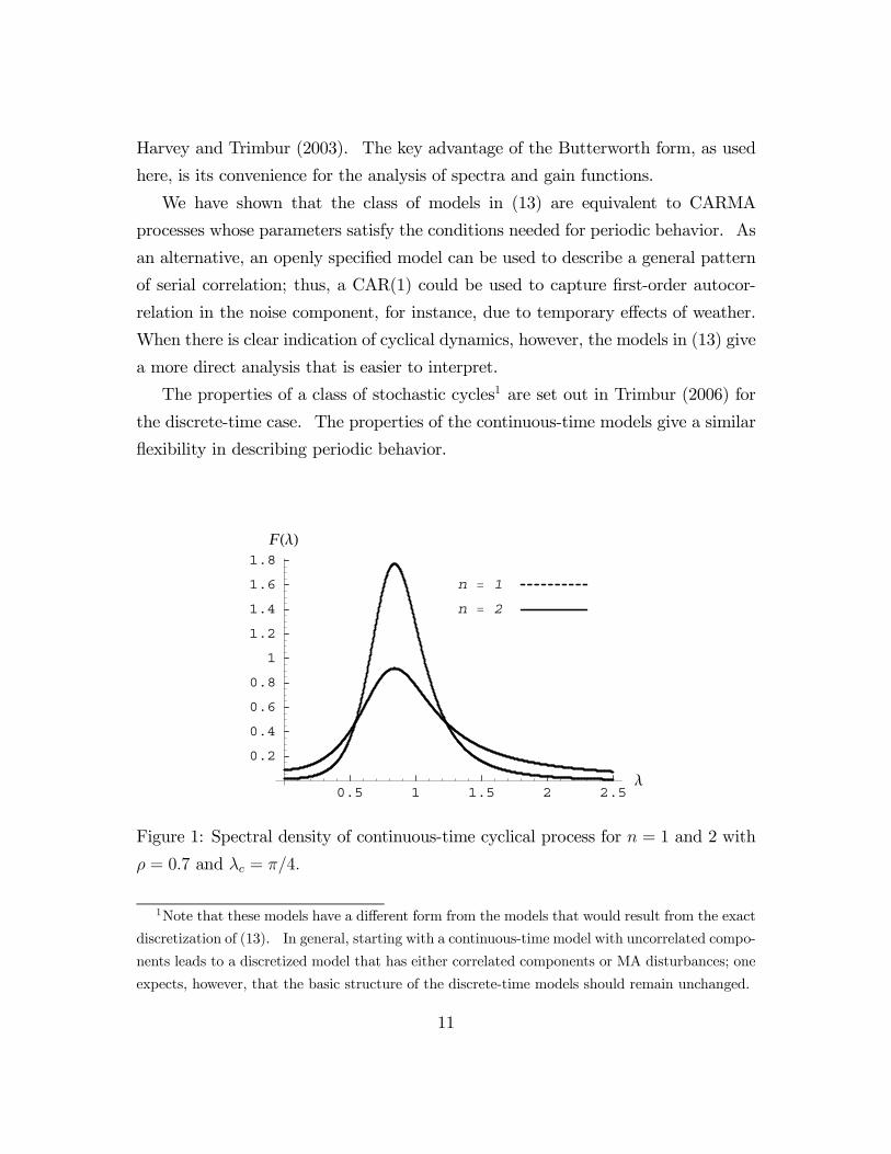
Figure 1: Spectral density of continuous-time cyclical process for = 1 and 2 with

= 07 and = 4

1Note that these models have a different form from the models that would result from the exact

discretization of (13). In general, starting with a continuous-time model with uncorrelated compo-

nents leads to a discretized model that has either correlated components or MA disturbances; one

expects, however, that the basic structure of the discrete-time models should remain unchanged.

11

Figure 1 shows the spectrum for parameter values = 4. In particular, the

function (22)−1(; ) is plotted, where the normalizing constant includes

the unconditional variance 2 of the cycle; this is computed in Mathematica by

numerical integration of the power spectrum for given values of and . For

= 1, the damping factor is set to = 09, and for = 2, it is set to = 075.

Lower values of are appropriate for the higher order models because of their

resonance property. Thus, the cyclical shocks reinforce the periodicity in (),

making the oscillations more persistent for given . The difference in spectra in

figure 1 indicates that the periodicity is more clearly defined for the second order

cycle.

The spectrum peaks at a period around 2 for moderate values of , say

5 which is the standard business cycle range. The maximum does

not occur exactly at = , however, except as tends to unity. The case = 1

gives a nonstationary cycle, where one could, in theory, forecast out to unlimited

horizons. Thus, in economic modeling, attention is usually restricted to stationary

models where 1.

3 Signal Extraction in Continuous Time

This section develops the signal extraction problem in continuous time. A new

result with proof is given for estimating a nonstationary signal from stationary

noise. Whittle (1983) shows a similar result for nonstationary processes, but omits

the proof and in particular, fails to recognize the importance of initial conditions.

Kailath, Sayed, and Hassibi (2000, p. 221 — 227) prove the formula for the special

case of a stationary signal. We extend the treatment of Whittle (1983) by providing

proofs, at the same time illustrating the importance of initial value assumptions to

the result. Further, the cases where the differentiated signal or noise process or both

are WN are treated rigorously.

12

3.1 Nonstationary signal and initial conditions

A key result of the paper is a proof of the signal extraction formula for nonstationary

models; this is crucial for many applications in economics. In discrete-time, methods

for nonstationary series rely on theoretical foundations, as set out in Bell (1984). In

this paper, we extend the Whittle (1983) result to the case of a nonstationary signal,

that is, integrated of order , where 0 is an integer. Consider the following

decomposition for a continuous time process ():

() = () + () ∈ R (17)

where () is stationary. The aim is to estimate the underlying signal () in the

presence of the noise, and it will be assumed that () ∼ () or integrated of order

.

In general, is any non-negative integer; the special case = 0 reduces to

stationary (). In many applications of interest, we have 0, so that the th

derivative of () denoted by (), is stationary. It is assumed that () and ()

are mean zero and uncorrelated with one another. In the standard case, both

autocovariance functions, and , are integrable. An extension could also

be considered where or or both are represented by a multiple of the Dirac

delta function, which gives rise to tempered distributions (see Folland, 1995); the

associated spectral densities are flat, indicating a corresponding WN process.

The process () satisfies the stochastic differential equation

() = () = () +() (18)

From Section 22, the spectral density of () is

() = () + 2() (19)

From Hannan (1970, p. 81), the nonstationary process () can be written in

terms of some initial values plus a -fold integral of the stationary (). For example,

when = 1,

() = (0) +

Z

0

()

13

for some initial value random variable (0). Note that this remains valid both for

0 and for 0. When = 2,

() = (0) + (0) +

Z

0

Z

0

()

for initial position (0) and velocity (0) = [](0). In general, we can write

() =−1X=0

!()(0) + []() (20)

with the operator defined by []() =R 0()(− )−1 ( − 1)!. Note that

(20) holds for the signal () as well, if we substitute for and for .

For an () process, let y∗(0) = {(0) (0) · · · (−1)(0)} denote the collectionof values and higher order derivatives at time = 0. It is assumed that y∗(0)

is uncorrelated with both () and () for all . This assumption is analogous to

Assumption A in Bell (1984), except that now higher order derivatives are involved.

3.2 Formula for the optimal filter

Consider the theoretical signal extraction problem for a bi-infinite series () that

follows (17). The optimal linear estimator of the signal () gives the minimum

mean square error. Thus, the goal is to minimize E[(()− ())2] such that

() = Ψ()() = ( ∗ )() for some weighting kernel . The notation Ψ()

for a continuous-lag filter was introduced earlier. The problem is to determine the

optimal choice of Ψ() for general nonstationary models of the form (17). The

following theorem shows the main result.

Theorem 1 For the process in (17), suppose that y∗(0) is uncorrelated with both

() and () for all . Also, assume that () and () are mean zero weakly

stationary processes that are uncorrelated with one another, with autocovariance

functions that are either integrable or given by constant multiples of the Dirac delta

function, interpreted as a tempered distribution. Let

() =()

()

14

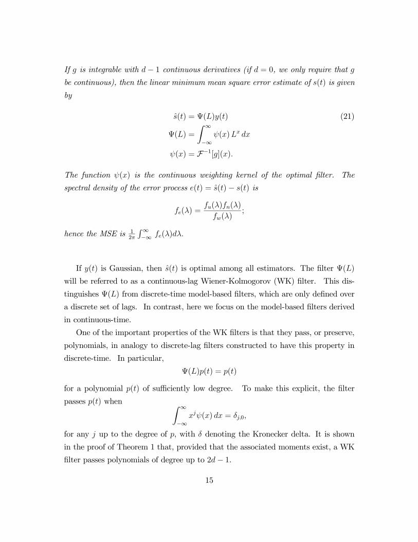
If is integrable with − 1 continuous derivatives (if = 0, we only require that be continuous), then the linear minimum mean square error estimate of () is given

by

() = Ψ()() (21)

Ψ() =

Z ∞

−∞()

() = F−1[]()

The function () is the continuous weighting kernel of the optimal filter. The

spectral density of the error process () = ()− () is

() =()()

();

hence the MSE is 12

R∞−∞ ()

If () is Gaussian, then () is optimal among all estimators. The filter Ψ()

will be referred to as a continuous-lag Wiener-Kolmogorov (WK) filter. This dis-

tinguishes Ψ() from discrete-time model-based filters, which are only defined over

a discrete set of lags. In contrast, here we focus on the model-based filters derived

in continuous-time.

One of the important properties of the WK filters is that they pass, or preserve,

polynomials, in analogy to discrete-lag filters constructed to have this property in

discrete-time. In particular,

Ψ()() = ()

for a polynomial () of sufficiently low degree. To make this explicit, the filter

passes () when Z ∞

−∞() = 0

for any up to the degree of , with denoting the Kronecker delta. It is shown

in the proof of Theorem 1 that, provided that the associated moments exist, a WK

filter passes polynomials of degree up to 2− 1.

15

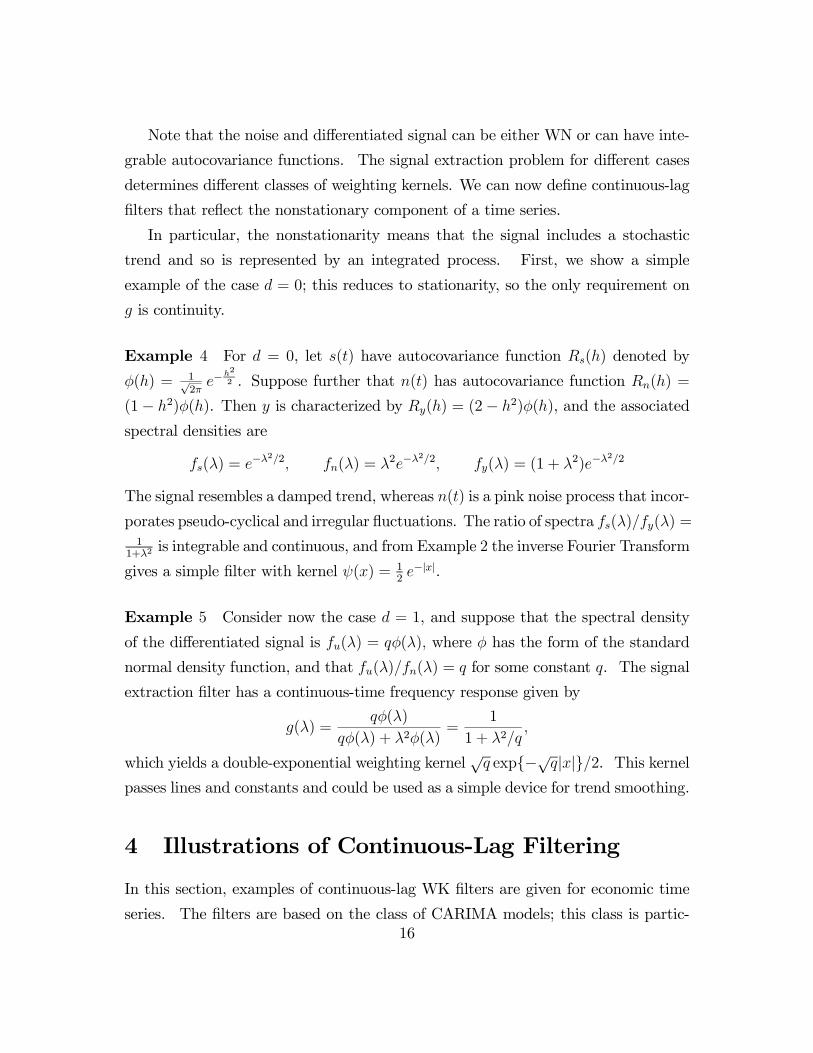
Note that the noise and differentiated signal can be either WN or can have inte-

grable autocovariance functions. The signal extraction problem for different cases

determines different classes of weighting kernels. We can now define continuous-lag

filters that reflect the nonstationary component of a time series.

In particular, the nonstationarity means that the signal includes a stochastic

trend and so is represented by an integrated process. First, we show a simple

example of the case = 0; this reduces to stationarity, so the only requirement on

is continuity.

Example 4 For = 0, let () have autocovariance function () denoted by

() = 1√2−

2

2 . Suppose further that () has autocovariance function () =

(1− 2)(). Then is characterized by () = (2− 2)(), and the associated

spectral densities are

() = −22 () = 2−

22 () = (1 + 2)−22

The signal resembles a damped trend, whereas () is a pink noise process that incor-

porates pseudo-cyclical and irregular fluctuations. The ratio of spectra ()() =1

1+2is integrable and continuous, and from Example 2 the inverse Fourier Transform

gives a simple filter with kernel () = 12−||.

Example 5 Consider now the case = 1, and suppose that the spectral density

of the differentiated signal is () = () where has the form of the standard

normal density function, and that ()() = for some constant . The signal

extraction filter has a continuous-time frequency response given by

() =()

() + 2()=

1

1 + 2

which yields a double-exponential weighting kernel√ exp{−√||}2. This kernel

passes lines and constants and could be used as a simple device for trend smoothing.

4 Illustrations of Continuous-Lag Filtering

In this section, examples of continuous-lag WK filters are given for economic time

series. The filters are based on the class of CARIMA models; this class is partic-

16

ularly convenient for computing WK weighting kernels and offers flexibility for a

range of applications. The spectral densities and that enter the formula for

the gain are both rational functions in 2. Taking their ratio yields another rational

function in 2 for () As these analytical expressions summarize the comprehen-

sive effects of the filter, they can be studied and used in filter design in different

contexts.

We focus on examples where CARIMA models are set up within different signal

extraction problems. The specifications are guided by applications of interest in

economics; their solutions rely on the theorem given in the last Section for handling

nonstationary series. It seems clear that many economic series show stochastic

trend, and recent research has shown that the implications of nonstationarity depend

on stock or flow sampling. For instance, Chambers (2004) has studied the properties

of unit root tests for flow observed series. In designing filters, we handle this

dependence by starting with fundamental filters set up in continuous-time.

In the first example, we consider the simplest case, the local level model. The

second example considers an extension of the well-known HP filter, which has been

widely used in macroeconomics as a detrending method. We show that the expres-

sion for the continuous-lag HP filter is relatively simple, and this gives a basis for

detrending data with different sampling conditions.

The third example extends the treatment with a derivation of continuous-lag low-

pass and band-pass Butterworth filters. This class of filters represents the analogue

of the discrete-time filters introduced in Harvey and Trimbur (2003). The band-

pass filters arise naturally as cycle estimators in a well-defined model that jointly

describes trend, cyclical, and noisy movements. The general cyclical processes in

continuous-time are defined in an analogous way to the discrete-time models studied

in Trimbur (2006). Note that the cyclical components are equivalent to certain

CARMA models. In the analysis of periodic behavior, it is more direct to work

with the structural form; the frequency parameter, for instance, reflects the average,

or central, periodicity.

The low-pass and band-pass filters we present have the property of mutual con-

sistency. That is, they may be applied simultaneously. Other procedures, in

contrast, do not preserve this property when the two filters are designed separately,

17

or when they are based on different source models.

It is generally straightforward to investigate the weighting kernels of the WK

filters. This involves calculating the residues of rational functions, a standard

problem for which well-known procedures are available. Still, the computations can

become burdensome in particular cases, so in presenting illustrations, we restrict

attention to some standard filters. In these cases, the derivation of analytical results

is feasible, with the expressions simple enough to provide a clear interpretation.

In the framework of WK filters, source models can be formulated to adapt to

different situations. For instance, some series of Industrial Output are subject to

weather effects that induce short-lived serial correlation. In estimating the trend,

the base model can be set up with a low-order CAR or CARMA component.

The approach to filter design can also be adapted to focus on certain properties

of the signal, such as rate of change. Thus, in a more general framework, our target

of estimation becomes a functional of the signal. This opens the door to a number

of potential applications, such as turning point analysis, where the interest centers

on some aspect of the signal’s evolution over an interval. After describing the basic

principle, in a fourth example, we examine an application to measuring velocity and

acceleration of signal.

Illustration 1: Local Level Model The trend plus noise model is written as

() = ()+() where () denotes the stochastic level, and () is continuous-time

white noise with variance parameter 2 , denoted by () ∼(0 2 ). See Harvey

(1989) for discussion. An interpretation of the variance 2 is that Θ()() has

autocovariance function ( ∗−)()2 for any (integrable) auxiliary weighting kernel.

The local level model assumes () = (), where () ∼ (0 2). The

signal-noise ratio in the continuous-time framework is defined as = 22 . So the

observed process () requires one derivative for stationarity, and we write () =

(). The spectral densities of the differentiated trend and observed process are

() = 2 () = () + 22 = ( + 2)2 (22)

Though the constant function () is nonintegrable over the real line, the frequency18

response of the signal extraction filter is given by the ratio (1 + 2)−1 which

is integrable. As in the previous example, the weighting kernel has the double

exponential shape:

() =

√

2exp{−√||}

The rate of decay in the tails now depends on the signal-noise ratio of the underlying

continuous-time model.

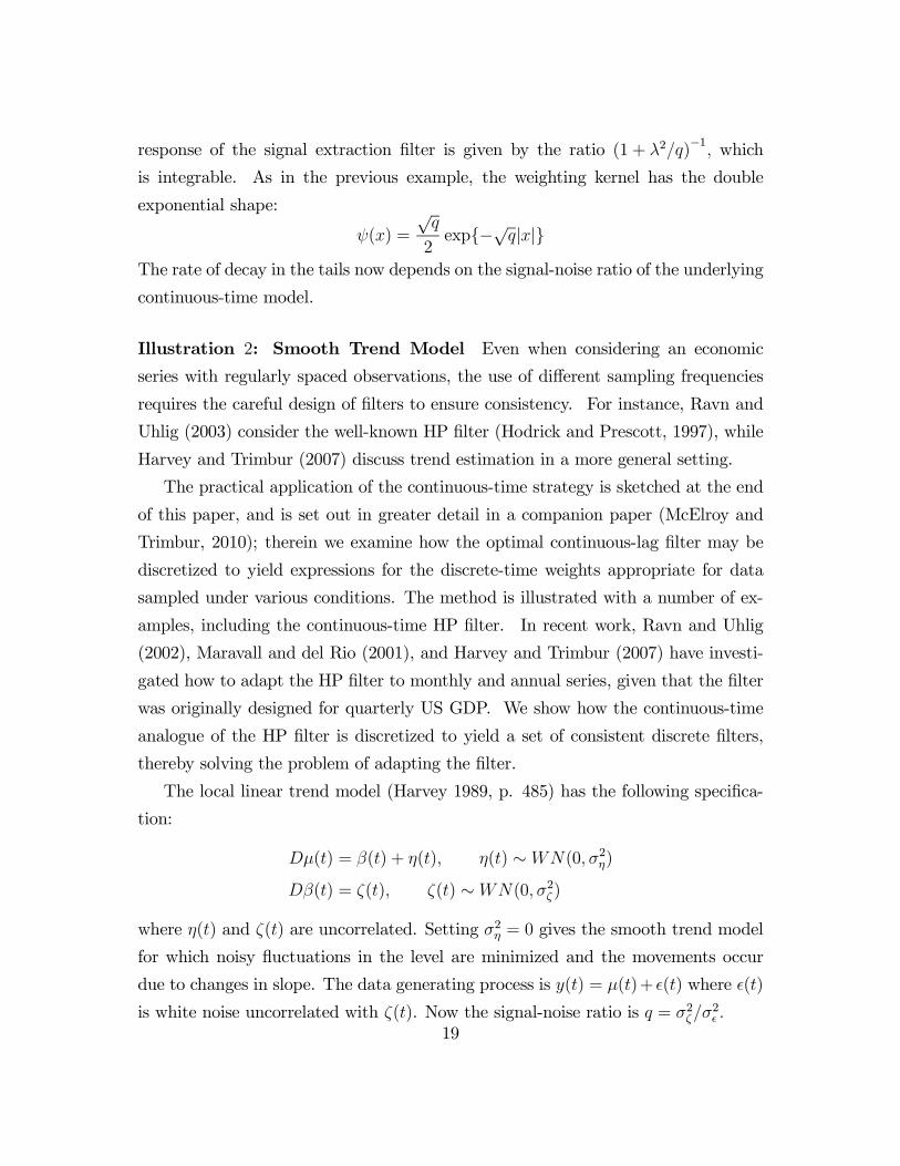
Illustration 2: Smooth Trend Model Even when considering an economic

series with regularly spaced observations, the use of different sampling frequencies

requires the careful design of filters to ensure consistency. For instance, Ravn and

Uhlig (2003) consider the well-known HP filter (Hodrick and Prescott, 1997), while

Harvey and Trimbur (2007) discuss trend estimation in a more general setting.

The practical application of the continuous-time strategy is sketched at the end

of this paper, and is set out in greater detail in a companion paper (McElroy and

Trimbur, 2010); therein we examine how the optimal continuous-lag filter may be

discretized to yield expressions for the discrete-time weights appropriate for data

sampled under various conditions. The method is illustrated with a number of ex-

amples, including the continuous-time HP filter. In recent work, Ravn and Uhlig

(2002), Maravall and del Rio (2001), and Harvey and Trimbur (2007) have investi-

gated how to adapt the HP filter to monthly and annual series, given that the filter

was originally designed for quarterly US GDP. We show how the continuous-time

analogue of the HP filter is discretized to yield a set of consistent discrete filters,

thereby solving the problem of adapting the filter.

The local linear trend model (Harvey 1989, p. 485) has the following specifica-

tion:

() = () + () () ∼(0 2)

() = () () ∼(0 2 )

where () and () are uncorrelated. Setting 2 = 0 gives the smooth trend model

for which noisy fluctuations in the level are minimized and the movements occur

due to changes in slope. The data generating process is () = ()+ () where ()

is white noise uncorrelated with (). Now the signal-noise ratio is = 22

19

�2�4�6�8�10 2 4 6 8 10x

0.1

0.2

w�x�

Continuous Time HP Filter

Weighting kernels

q � 1�10

q � 1�40

q � 1�200

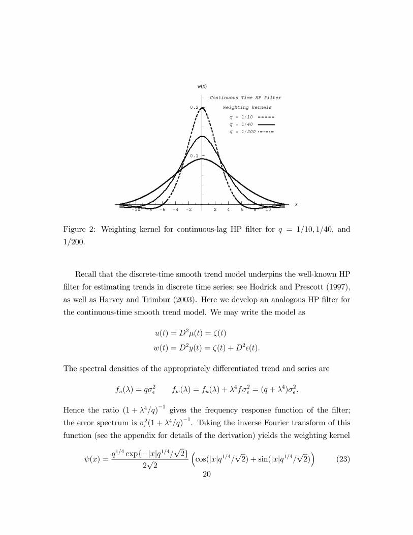
Figure 2: Weighting kernel for continuous-lag HP filter for = 110 140 and

1/200.

Recall that the discrete-time smooth trend model underpins the well-known HP

filter for estimating trends in discrete time series; see Hodrick and Prescott (1997),

as well as Harvey and Trimbur (2003). Here we develop an analogous HP filter for

the continuous-time smooth trend model. We may write the model as

() = 2() = ()

() = 2() = () +2()

The spectral densities of the appropriately differentiated trend and series are

() = 2 () = () + 42 = ( + 4)2

Hence the ratio (1 + 4)−1gives the frequency response function of the filter;

the error spectrum is 2 (1 + 4)−1. Taking the inverse Fourier transform of this

function (see the appendix for details of the derivation) yields the weighting kernel

() =14 exp{−||14√2}

2√2

³cos(||14

√2) + sin(||14

√2)´

(23)

20

This gives the continuous-time extension of the HP filter. From the discussion

following Theorem 1, the kernel in (23) passes cubics.

Figure 2 shows the weighting function for three different values of . As the

signal-noise ratio increases, the trend becomes more variable relative to noise, so

the resulting kernel places more emphasis on nearby observations. Similarly, as

decreases, the filter adapts by smoothing over a wider range. The negative side-

lobes, apparent in the figure for = 110 enable the filter to pass quadratics and

cubics.

Illustration 3: Continuous-Lag Band-Pass A second result is the development

of a class of continuous-lag Butterworth filters for economic data. In particular, we

introduce low-pass and band-pass filters in continuous-time that are analogous to

the filters derived by Harvey and Trimbur (2003) for the corresponding discrete-time

models, and their properties are illustrated through plots of the continuous-time gain

functions. One special case of interest is the derivation of a continuous-lag filter from

the smooth trend model; this gives a continuous-time extension of the popular HP

filter. At the root of the model-based band-pass is a class of higher order cycles in

continuous-time. This class generalizes the stochastic differential equation (SDE)

model for a stochastic cycle developed in Harvey (1989) and Harvey and Stock

(1993).

Consider again the class of stochastic cycles in Example 3. A simple (nonsea-

sonal) model for a continuous-time process in macroeconomics is given by

() = () + () + ()

where () is a trend component that accounts for long-term movements and the

cyclical component () follows (13) for index . The irregular () is meant to

absorb any random, or nonsystematic variation, and in direct analogy with discrete-

time, it is assumed that in continuous-time, () ∼ (0 2). The definition of

the −th order trend is

() = () () ∼(0 2 )

21

for integer 0. For = 1, this gives standard Brownian motion. For = 2

() is integrated Brownian motion, the continuous-time analogue of the smooth

trend, as in the previous illustration.

In formulating the estimation of () as a signal extraction problem, we set the

nonstationary signal to () + () and the ‘noise’ to (). This is done just to

map the estimation problem to the framework developed in the last Section; it is

not intended to suggest any special importance of ‘signal’ as a target of extraction.

Actually in this case, the ‘noise’ part will usually be of greatest interest in a business

cycle analysis. Thus, the optimal filter () is constructed for ()+(), and the

complement of this filter, (1− ()) yields the band-pass. Similarly, to formulate

the estimation of (), take () = () and () = () + ().

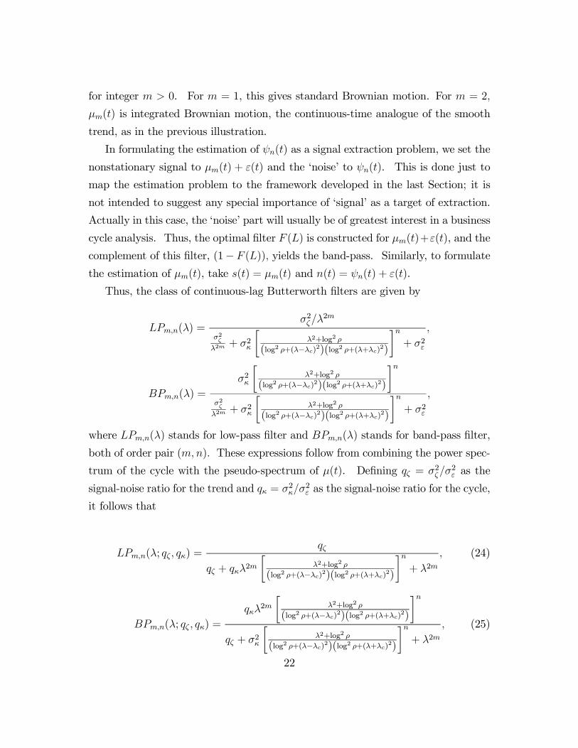
Thus, the class of continuous-lag Butterworth filters are given by

() =2

2

22

+ 2

∙2+log2

(log2 +(−)2)(log2 +(+)2)

¸+ 2

() =

2

∙2+log2

(log2 +(−)2)(log2 +(+)2)

¸22

+ 2

∙2+log2

(log2 +(−)2)(log2 +(+)2)

¸+ 2

where () stands for low-pass filter and () stands for band-pass filter,

both of order pair () These expressions follow from combining the power spec-

trum of the cycle with the pseudo-spectrum of (). Defining = 22 as the

signal-noise ratio for the trend and = 22 as the signal-noise ratio for the cycle,

it follows that

(; ) =

+ 2∙

2+log2

(log2 +(−)2)(log2 +(+)2)

¸+ 2

(24)

(; ) =

2

∙2+log2

(log2 +(−)2)(log2 +(+)2)

¸ + 2

∙2+log2

(log2 +(−)2)(log2 +(+)2)

¸+ 2

(25)

22

Here the order = denotes the order of integration as determined by the stochas-

tic trend model. The definitions in (24) and (25) parallel the development of Harvey

and Trimbur (2003) for the discrete-time case. Note that in the continuous-time

case, we must have integrability of the frequency response function over the entire

real line rather than over a restricted interval.

0.5 1 1.5 2 2.5Λ

0.2

0.4

0.6

0.8

1

G�Λ�

Low�Pass

Band�Pass

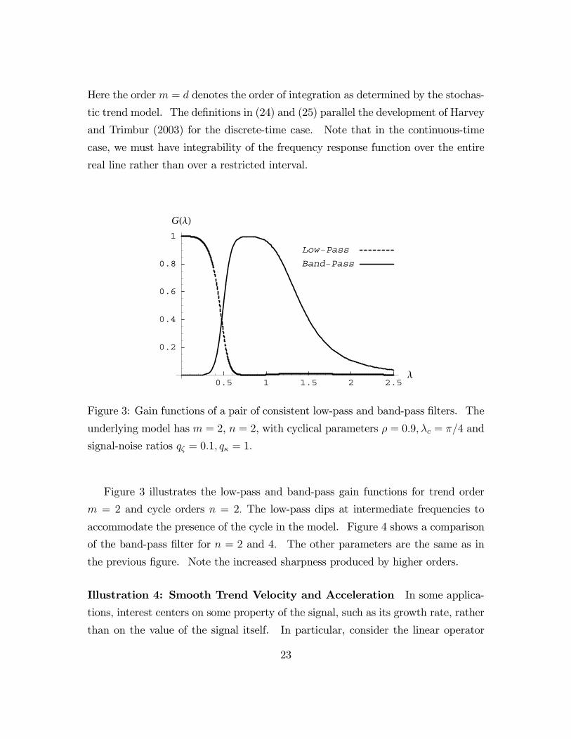
Figure 3: Gain functions of a pair of consistent low-pass and band-pass filters. The

underlying model has = 2, = 2, with cyclical parameters = 09 = 4 and

signal-noise ratios = 01 = 1

Figure 3 illustrates the low-pass and band-pass gain functions for trend order

= 2 and cycle orders = 2 The low-pass dips at intermediate frequencies to

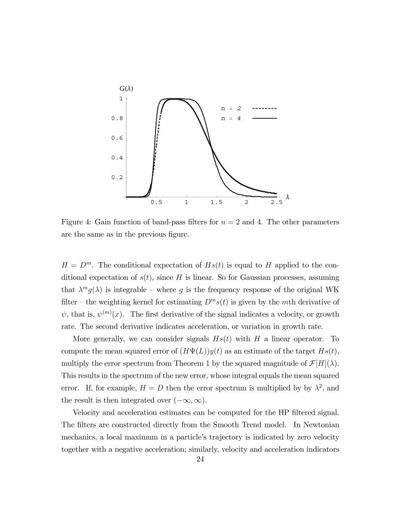
accommodate the presence of the cycle in the model. Figure 4 shows a comparison

of the band-pass filter for = 2 and 4. The other parameters are the same as in

the previous figure. Note the increased sharpness produced by higher orders.

Illustration 4: Smooth Trend Velocity and Acceleration In some applica-

tions, interest centers on some property of the signal, such as its growth rate, rather

than on the value of the signal itself. In particular, consider the linear operator

23

0.5 1 1.5 2 2.5Λ

0.2

0.4

0.6

0.8

1

G�Λ�

n � 2

n � 4

Figure 4: Gain function of band-pass filters for = 2 and 4. The other parameters

are the same as in the previous figure.

= . The conditional expectation of () is equal to applied to the con-

ditional expectation of (), since is linear. So for Gaussian processes, assuming

that () is integrable — where is the frequency response of the original WK

filter — the weighting kernel for estimating () is given by the th derivative of

, that is, ()(). The first derivative of the signal indicates a velocity, or growth

rate. The second derivative indicates acceleration, or variation in growth rate.

More generally, we can consider signals () with a linear operator. To

compute the mean squared error of (Ψ())() as an estimate of the target (),

multiply the error spectrum from Theorem 1 by the squared magnitude of F []().This results in the spectrum of the new error, whose integral equals the mean squared

error. If, for example, = then the error spectrum is multiplied by by 2, and

the result is then integrated over (−∞∞).Velocity and acceleration estimates can be computed for the HP filtered signal.

The filters are constructed directly from the Smooth Trend model. In Newtonian

mechanics, a local maximum in a particle’s trajectory is indicated by zero velocity

together with a negative acceleration; similarly, velocity and acceleration indicators

24

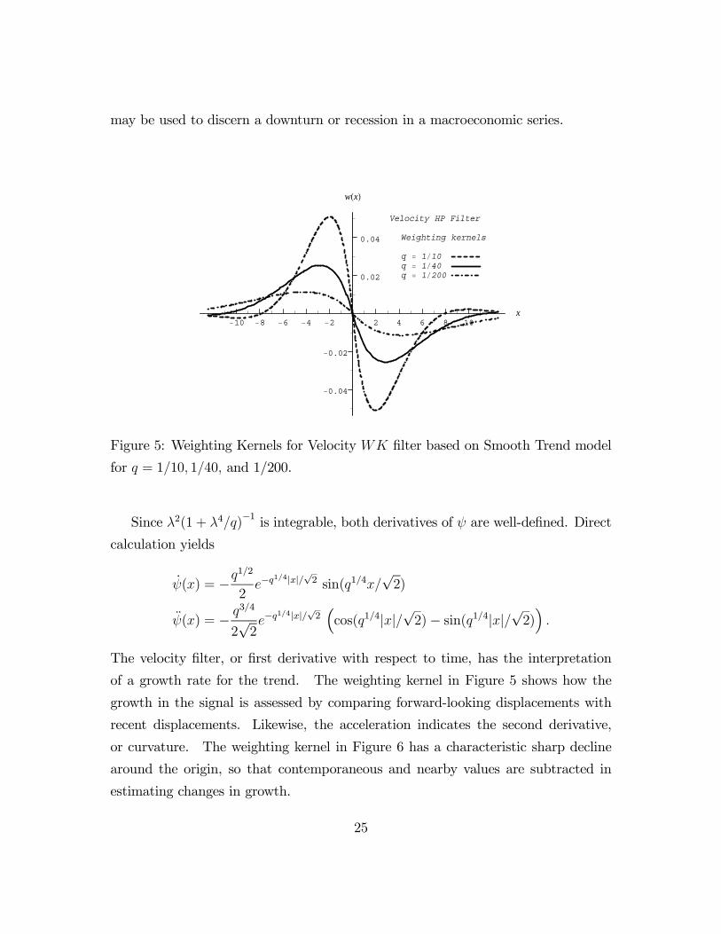
may be used to discern a downturn or recession in a macroeconomic series.

�2�4�6�8�10 2 4 6 8 10x

w�x�

Weighting kernels

Velocity HP Filter

q � 1�10q � 1�40q � 1�2000.02

0.04

�0.02

�0.04

Figure 5: Weighting Kernels for Velocity filter based on Smooth Trend model

for = 110 140 and 1/200.

Since 2(1 + 4)−1is integrable, both derivatives of are well-defined. Direct

calculation yields

() = −12

2−

14||√2 sin(14√2)

() = − 34

2√2−

14||√2³cos(14||

√2)− sin(14||

√2)´

The velocity filter, or first derivative with respect to time, has the interpretation

of a growth rate for the trend. The weighting kernel in Figure 5 shows how the

growth in the signal is assessed by comparing forward-looking displacements with

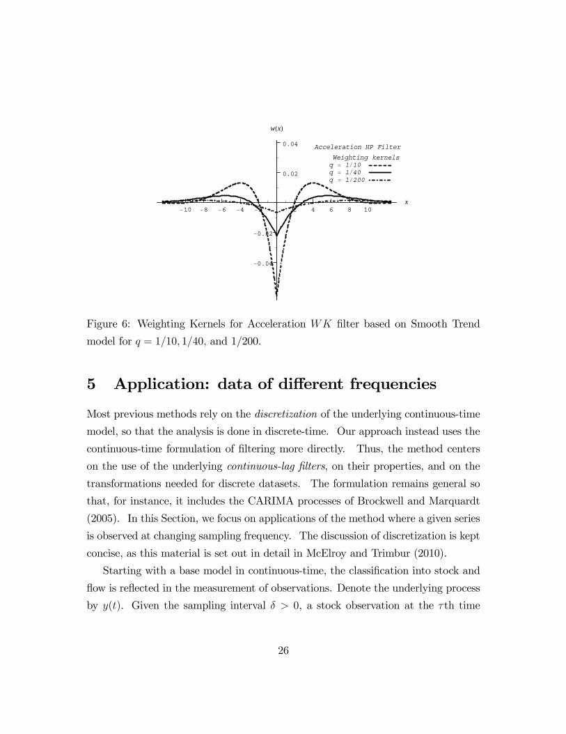
recent displacements. Likewise, the acceleration indicates the second derivative,

or curvature. The weighting kernel in Figure 6 has a characteristic sharp decline

around the origin, so that contemporaneous and nearby values are subtracted in

estimating changes in growth.

25

�2�4�6�8�10 2 4 6 8 10x

w�x�

Weighting kernels

Acceleration HP Filter

q � 1�10q � 1�40q � 1�200

0.02

0.04

�0.02

�0.04

Figure 6: Weighting Kernels for Acceleration filter based on Smooth Trend

model for = 110 140 and 1/200.

5 Application: data of different frequencies

Most previous methods rely on the discretization of the underlying continuous-time

model, so that the analysis is done in discrete-time. Our approach instead uses the

continuous-time formulation of filtering more directly. Thus, the method centers

on the use of the underlying continuous-lag filters, on their properties, and on the

transformations needed for discrete datasets. The formulation remains general so

that, for instance, it includes the CARIMA processes of Brockwell and Marquardt

(2005). In this Section, we focus on applications of the method where a given series

is observed at changing sampling frequency. The discussion of discretization is kept

concise, as this material is set out in detail in McElroy and Trimbur (2010).

Starting with a base model in continuous-time, the classification into stock and

flow is reflected in the measurement of observations. Denote the underlying process

by (). Given the sampling interval 0, a stock observation at the th time

26

point is defined as

= () (26)

The times of observations correspond to = for integer . The discrete

stock time series is then the sequence of values {}∞=−∞.A series of flow observations has the form

=

Z

(−1)() (27)

where is both the interval of cumulation and the interval separating successive

observation points. Note that, more generally, the times ...,1 2 · · · ,... neednot be equally spaced, but for now we assume for simplicity that the spacing is

constant at − −1 = .

McElroy and Trimbur (2010) applied continuous-lag filters to the total, or head-

line, inflation rate, in particular the consumer price index (Source: Bureau of Labor

Statistics). However, policymakers and economic analysts often follow the move-

ments in the less volatile components of inflation as these can provide a closer in-

dication of basic price trends in the macroeconomy. The core CPI index subtracts

out two sectors with a high degree of idiosyncratic movements, that is, food and

energy. Nevertheless, the core index can adjust rapidly during times of economic

transition, making it a challenge to get a useful signal about underlying patterns.

This provides a practical reason for our interest in trend filters for removing the

nonsystematic noise, and furthermore, the simple underlying models may provide a

helpful starting point for analysis. The estimated signal is tailored to the charac-

teristics of core inflation, that is, the trend dynamics relative to irregular, and in

this paper to the frequency of observation as well.

We can view the prices of different products as staggered menus, with each up-

dated periodically. At a given time, certain goods are subject to changing prices,

so the average level representative of the overall economy evolves constantly. De-

note the aggregate price level at time by () Consider a simple model for the

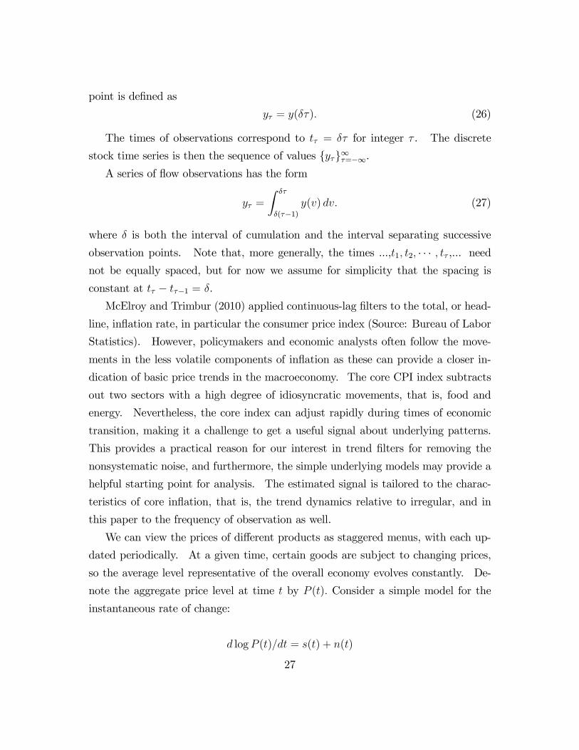
instantaneous rate of change:

log () = () + ()

27

where signal and noise have the form (22). A random walk is often used for trend

inflation in econometric modelling, so we carry this assumption to filter design in

continuous-time, with the signal denoting Brownian motion.

Given a sampling interval the inflation rate at time = is

= (100)× log(1 + ∗)

where ∗ is the straight percent change in prices from − to That is, ∗ =

( () − ( − )) ( − ) − 1 This definition follows Stock and Watson (1999).Using this transformation, analogous to taking log-returns for asset prices, allows

for analysis independent of sampling frequency.

Now the inflation rate may be written as

= (100)× log[ () (− )] = (100)× (log ()− log (− ))

= (100)

Z

(−1)( log ())

so the observations are constructed as in (27). That is, the flow observations are

based on cumulative sampling of the continuous process log.

To compute estimates of the continuous-time variance parameters, we set up

the likelihood function for highest frequency available (monthly) and use maximum

likelihood. The likelihood function comes from the discrete-time local level model

implied by the CT model, as shown in Harvey and Trimbur (2007). The sample

period is January 1960 to January 2009. We used a program written in the Ox

language (Doornik, 2009) with the SsfPack routines (Koopman et. al, 2006) that

estimated the model by applying maximum likelihood to the state space. The

estimates of the continuous-time variance parameters give the ratio = 22 =

4664

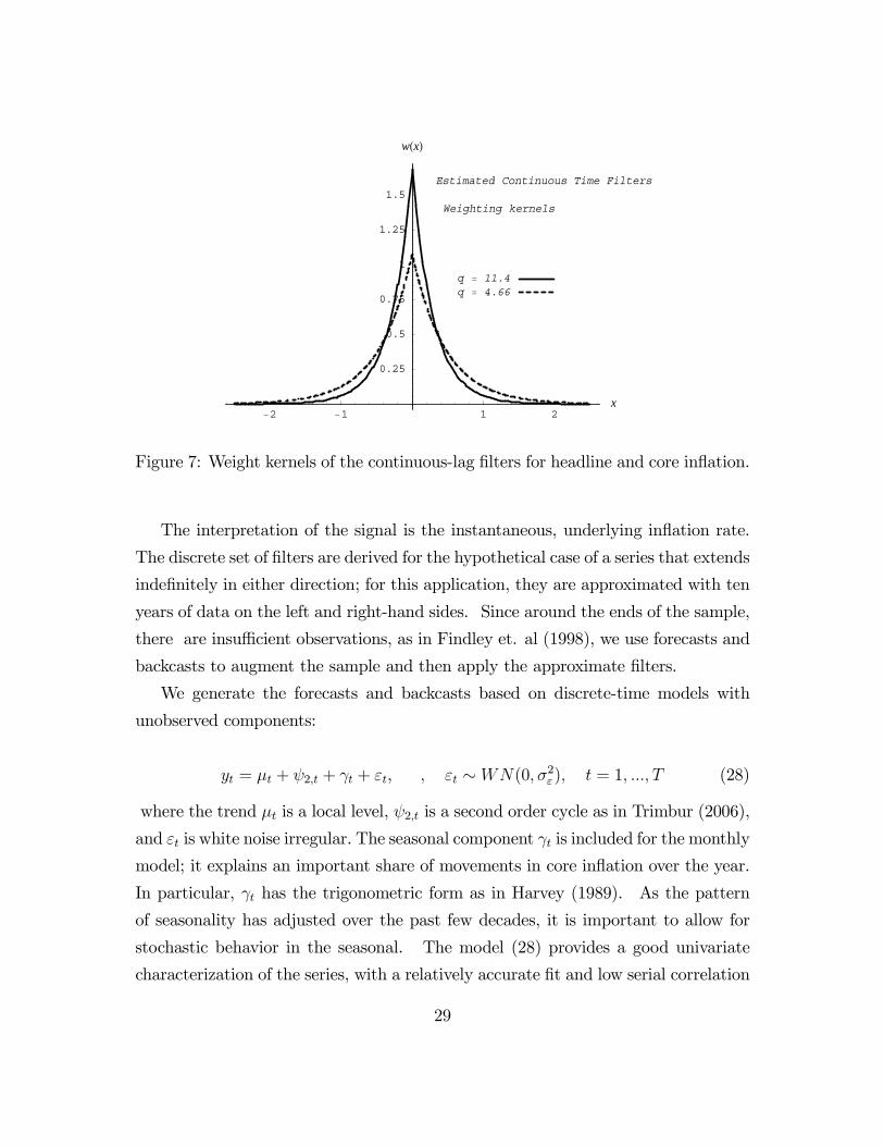
Figure 7 compares the continuous-lag filter for the core inflation rate investigated

here with the one for the headline inflation rate examined in McElroy and Trimbur

(2010). A smaller parameter for the signal in core inflation means that more

weight is spread across previous and past observations in gauging the current signal.

In contrast, for headline inflation, the trend tends to change more rapidly, so the

smoothing emphasizes the current and nearby data points.

28

�2 �1 1 2x

0.25

0.5

0.75

1

1.25

1.5

w�x�

Estimated Continuous Time Filters

Weighting kernels

q � 11.4q � 4.66

Figure 7: Weight kernels of the continuous-lag filters for headline and core inflation.

The interpretation of the signal is the instantaneous, underlying inflation rate.

The discrete set of filters are derived for the hypothetical case of a series that extends

indefinitely in either direction; for this application, they are approximated with ten

years of data on the left and right-hand sides. Since around the ends of the sample,

there are insufficient observations, as in Findley et. al (1998), we use forecasts and

backcasts to augment the sample and then apply the approximate filters.

We generate the forecasts and backcasts based on discrete-time models with

unobserved components:

= + 2 + + , ∼(0 2) = 1 (28)

where the trend is a local level, 2 is a second order cycle as in Trimbur (2006),

and is white noise irregular. The seasonal component is included for the monthly

model; it explains an important share of movements in core inflation over the year.

In particular, has the trigonometric form as in Harvey (1989). As the pattern

of seasonality has adjusted over the past few decades, it is important to allow for

stochastic behavior in the seasonal. The model (28) provides a good univariate

characterization of the series, with a relatively accurate fit and low serial correlation

29

in the residuals.

There are various reasons for having an interest in different sampling frequencies.

First, we may have some indicators that are only available at coarser intervals, while

others are published more often. If we want to link the signals in the indicators and

the target series, then to maintain consistency, we can look at the target signal at

the various frequencies. For instance, if one indicator for core inflation is monthly

(e.g., capacity utilization) while another indicator is annual (say real GDP prior

to 1947), then can look at relationships between indicator and target in a unified

application.

A second reason is that a given series, or closely related series, may be available

over different sample periods for different frequencies of observation. As an exam-

ple, real GDP data was published quarterly for a sample starting in 1947. However,

annual data has been reported farther back. This information might be of interest

if we want to include the different kinds of business cycle movements that occurred

before WWII. Our consistent filter design gives a rigorous approach to studying

the underlying signal in both series. A third motivation is that series of different

sampling frequency naturally have some different information; the process of aggre-

gation functions like a very simple smoother that leads to more concentration on

the longer-run. Even though, strictly speaking, the lower frequency involves a loss

of some short-term information, it can end up making certain properties more easily

studied, such as turning points.

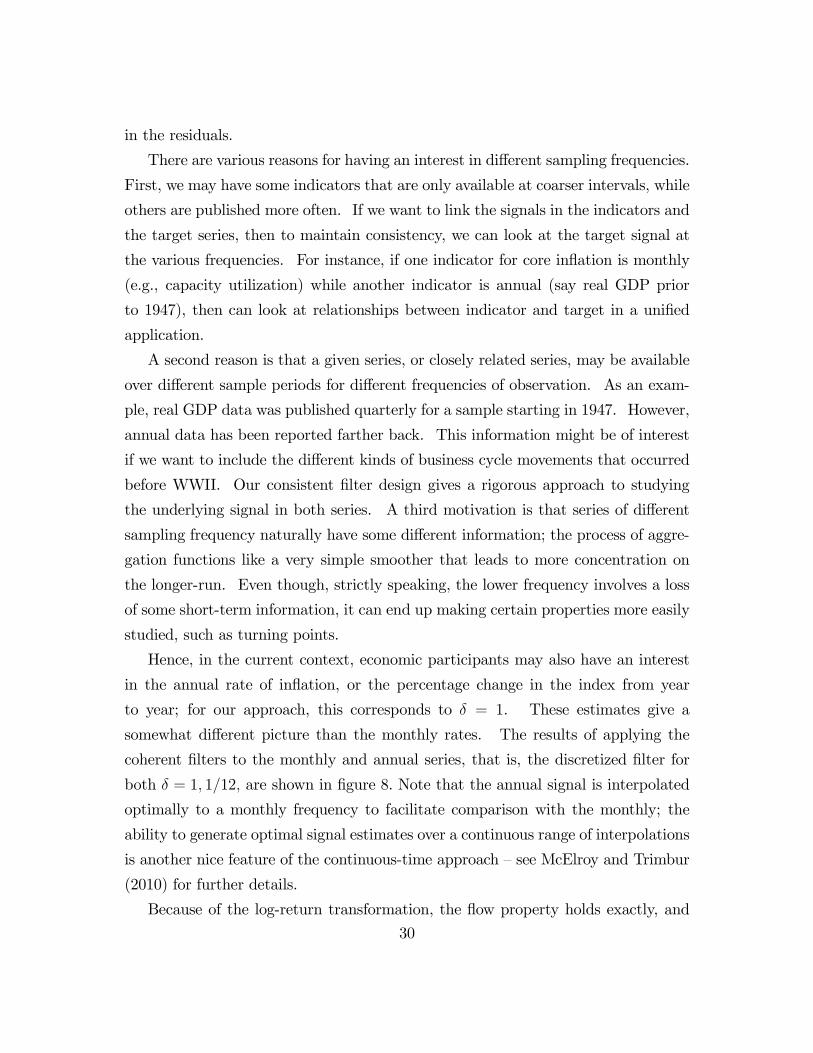
Hence, in the current context, economic participants may also have an interest

in the annual rate of inflation, or the percentage change in the index from year

to year; for our approach, this corresponds to = 1. These estimates give a

somewhat different picture than the monthly rates. The results of applying the

coherent filters to the monthly and annual series, that is, the discretized filter for

both = 1 112 are shown in figure 8. Note that the annual signal is interpolated

optimally to a monthly frequency to facilitate comparison with the monthly; the

ability to generate optimal signal estimates over a continuous range of interpolations

is another nice feature of the continuous-time approach — see McElroy and Trimbur

(2010) for further details.

Because of the log-return transformation, the flow property holds exactly, and

30

Monthly Signal Annual Signal

1960 1970 1980 1990 2000

2

4

6

8

10Monthly Signal Annual Signal

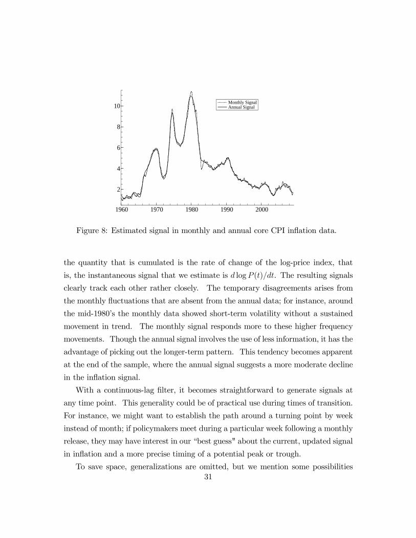
Figure 8: Estimated signal in monthly and annual core CPI inflation data.

the quantity that is cumulated is the rate of change of the log-price index, that

is, the instantaneous signal that we estimate is log (). The resulting signals

clearly track each other rather closely. The temporary disagreements arises from

the monthly fluctuations that are absent from the annual data; for instance, around

the mid-1980’s the monthly data showed short-term volatility without a sustained

movement in trend. The monthly signal responds more to these higher frequency

movements. Though the annual signal involves the use of less information, it has the

advantage of picking out the longer-term pattern. This tendency becomes apparent

at the end of the sample, where the annual signal suggests a more moderate decline

in the inflation signal.

With a continuous-lag filter, it becomes straightforward to generate signals at

any time point. This generality could be of practical use during times of transition.

For instance, we might want to establish the path around a turning point by week

instead of month; if policymakers meet during a particular week following a monthly

release, they may have interest in our “best guess" about the current, updated signal

in inflation and a more precise timing of a potential peak or trough.

To save space, generalizations are omitted, but we mention some possibilities

31

briefly. Seasonal components could be set up in continuous-time, and then the

resulting filter would give a unified basis for deriving seasonal filters at different

frequencies. Therefore, the adjusted series would be coherent across monthly and

quarterly (and perhaps even weekly) observations. Further, in continuous-time,

different trends and stationary CARMA processes could be used for more general fil-

ters. It seems possible that continuous-time specifications associated with dynamic

stochastic general equilibrium models could be formulated so the signal extraction

filters could be designed in a way consistent across frequencies. For instance, equi-

librium output under flexible prices or average levels of resource utilization could be

computed at monthly or quarterly frequencies in the proper way.

To handle the endpoint problem, we used forecast and backcast extension with a

model that accounted for the cyclical pattern and serial correlation in the inflation

rate. The filters are based on the simple local level model whose parameters are

inferred by fitting the discretized model to the highest frequency series. A further

extension of the adaptive filter design could find the optimal asymmetric filters near

the ends of sample, though this would prove a challenge in practice.

Our method opens the door to a wide range of possible applications. The weight-

ing kernels can be computed for any models of the SDE form and so can be handled

analytically. Filters designed from more sophisticated models would be based on

the same principles. Another extension would be to use an auxiliary indicator,

such as commodity price data, available at daily or weekly intervals to refine the

interpolation. Filters based on multivariate models may be constructed in the same

way as the univariate filters.

The use of the continuous-lag filter leads to coherent discrete filters. Note that

if one were to determine filters separately for monthly and annual cases, then this

property will not generally hold. Since, however, we start with the filter , and

discretize the filter directly, then the coherency property does hold. Details may be

found in McElroy and Trimbur (2010). For now, it should be emphasized that our

approach, based on a continuous-lag kernel, can handle signal estimation in a rather

general context, that is, with an unequally spaced series of stock or flow data, and

a with a signal time point lying in between observation times. This generality of

the signal extraction problem cannot be achieved in a purely discrete-time setting

32

and could only possibly be achieved, with great difficulty, in an approach requiring

full model discretization.

6 Conclusion

Our proof of the signal extraction formula paves the way for the development and

application of continuous-lag filters in econometrics. This establishes the theo-

retical foundation for continuous-time signal extraction with nonstationary models.

We have introduced various continuous-lag filters, including Butterworth low-pass

and band-pass filters as well as velocity and acceleration filters for turning point

analysis.

The methods used in Harvey and Stock (1993) provide a benchmark for estima-

tion of continuous-time models. In designing filters, however, we have suggested a

different route that avoids the need to discretize the model for each case of discrete

sampling. A separate paper (McElroy and Trimbur, 2010) has concentrated on the

discretization of filters, where interest centers on extracting coherent signals across

the different series of observations. The discrete filters have internal consistency

across situations of unequal spacing, stock or flow sampling, missing data, and mixed

frequency data.

Our suggested strategy is to design continuous-lag filters by estimating the signal

extraction model according to Harvey and Stock (1993), and second, to discretize the

filters for application to real data. In the illustration, we have matched the trends

for monthly and annual inflation, but we stress the generality of the approach. Any

of the filters described in Section 3 or newly designed filters could be discretized to

handle different sampling conditions and interpolation. The target of estimation

may represent some function of the series, such as smoothed rate of change, and one

may consider multivariate models with indicator series (perhaps of higher frequency

than the series of interest).

Acknowledgements. The authors thank David Findley for helpful comments and

discussion.

33

Appendix: Proofs

Proof of Theorem 1. Throughout, we shall assume that 0, since the = 0

case is essentially handled in Kailath et al. (2000). In order to prove the theorem,

it suffices to show that the error process () = () − () is orthogonal to the

underlying process (). By (20), it suffices to show that () is orthogonal to ()

and the initial values ∗. So we begin by analyzing the error process produced by

the proposed weighting kernel = F−1[]. We first note the following interestingproperty of . The moments of Z

() =

()

()|=0

for exist by the smoothness assumptions on , and are easily shown to

equal zero if 0 2 (i.e., for ≤ 2, the moments are zero so long as

they exist — their existence is not guaranteed by the assumptions of the theorem).

Moreover, the integral of is equal to 1 if 0. These properties ensure (when

0) that the filter Ψ() passes polynomials of degree less than This is because

Ψ() = for . We first note that representation (20) also extends to the

signal: () =P−1

=0

!()(0) + []() Then the error process is

() = ( ∗ )()− () = ( ∗ )()− () + ( ∗ )()Since Ψ() passes polynomials, ( ∗ )()− () =

R(()−∆0())[

](− ) ,

where ∆0 is the Dirac delta function. Note that any filter that does not pass polyno-

mials cannot be MSE optimal, since the error process will grow unboundedly with

time. So we have

() =

Z(()−∆0())[

](− ) +

Z()(− )

which is orthogonal to ∗ by Assumption A. Due to the representation (20), it is

sufficient to show that the error process is uncorrelated with [](). For any real

E[()(+ )] =

Z(()−∆0())E

¡[](− )[](+ )

¢ (A.1)

+

Z()E

"(− )

Ã(− )−

−1X=0

(+ )

!()(0)

!#

34

which uses the fact that []() = []() + ()−P−1=0

!()(0). Now we have

E£[](− )[](+ )

¤=

Z −

0

Z +

0

(− − )−1(+ − )−1

(− 1)!2 (−) (A.2)

If is integrable, we can write () =12

R()

. If ∝ ∆0 instead, then

∝ 1; we can still use the above Fourier representation of in (A.2), because the

various integrals will take care of the non-integrability of automatically. SinceR 0 = (1− )(), we obtain that (A.2) is equal to

1

2

Z()

−2Ã−(−) −

−1X=0

(−)!

(− )!Ã

(−) −−1X=0

()

!(− )

!

When integrated against ()−∆0(), we use the moments property of to obtain

1

2

Z()

−2Ã−(−) −

−1X=0

(−)!

(− )!¡

Ψ(−)− ¢

=1

2

Z()

−()()

à −

−1X=0

(−)!

(− )

!

This uses Ψ(−) − 1 = −2()(), which is not integrable if ∝ 1; yet will be integrable under the conditions of the theorem. As for the noise

term in (A.1), we first note that ()() exists for each since () exists

by assumption; this existence is interpreted in the sense of Generalized Random

Processes (Hannan, 1970). In particularZ()E[(− )(− )] =

Z()(− ) =

1

2

Z()

Ψ(−)

This Fourier representation is valid even when ∝ 1, since Ψ(−) is integrableby assumption. Similarly,

E[(− )()(0)] =

E[(− )()]|=0 =

(− − )|=0 =

(− )

where the derivatives are interpreted in the sense of distributions — i.e., when this

quantity is integrated against a suitably smooth test function, the derivatives are

passed over via integration by parts:Z()E[(− )()(0)] = (−1)

Z()()(− )

35

Since Ψ(−) for is integrable by assumption, we have ()() = 12

R()Ψ(−) ,

and the second term in (A.1) becomes

1

2()Ψ(

−)

à −

−1X=0

(−)(− )

!

!

This cancels with the first term of (A.1), which shows that Ψ() is MSE optimal.

Using similar techniques, the error spectral density is obtained as well. ¤

Derivation of the Weighting Kernel in Illustration 2. We compute the

Fourier Transform via the Cauchy Integral Formula (Ahlfors, 1979), letting = 1

for simplicity:1

2

Z ∞

−∞

1

1 + 4−

We can replace by || because the integrand is even. The standard approach is tocompute the integral of the complex function

() =||

1 + 4

along the real axis by computing the sum of the residues in the upper half plane,

and multiplying by 2 (since is bounded and integrable in the upper half plane).

It has two simple poles there: 4 and 34. The residues work out to be

( − 4)()|4 =−||(1−)

√2

4(1 + )√2

( − 34)()|34 =−||(1+)

√2

4(1− )√2

respectively. Summing these and multiplying by gives the desired result, after

some simplification. To extend beyond the = 1 case, simply let 7→ 14 and

multiply by 14 by change of variable. ¤

36

References

[1] Ahlfors, L., 1979, Complex Analysis. McGraw-Hill, New York.

[2] Bell, W., 1984, Signal extraction for nonstationary time series. The Annals of

Statistics 12, 646 — 664.

[3] Bergstrom, A. R., 1988, The History of Continuous-Time Econometric Models.

Econometric Theory 4, 365-383.

[4] Bergstrom, A. R., 1990, Continuous Time Econometric Modelling. Oxford Uni-

versity Press, New York.

[5] Brockwell, P., 2001, Lévy-Driven CARMA Processes. Annals of the Institute

of Statistical Mathematics 53, 113—124.

[6] Brockwell, P. and T. Marquardt, 2005, Lévy-Driven and Fractionally Integrated

ARMA Processes with Continuous Time Parameter. Statistica Sinica 15, 477-

494.

[7] Chambers, M., 2004, Testing for Unit Roots with Flow Data and Varying Sam-

pling Frequency. Journal of Econometrics 119, 1—18.

[8] Chambers, M. and J. McGarry, 2002, Modeling Cyclical Behavior With

Differential-Difference Equations in an Unobserved Components Framework.

Econometric Theory 18, 387—419.

[9] Folland, G., 1995, Introduction to Partial Differential Equations. Princeton

University Press, Princeton.

[10] Gandolfo, G., 1993, Continuous Time Econometrics. Chapman and Hall, Lon-

don.

[11] Hannan, E., 1970, Multiple Time Series. Wiley, New York.

[12] Harvey, A. and J. Stock, J., 1985, The Estimation of Higher-Order Continuous-

Time Autoregressive Models. Econometric Theory 1, 97-117.

37

[13] Harvey, A. and J. Stock, 1993, Estimation, Smoothing, Interpolation, and Dis-

tribution for Structural Time-Series Models in Continuous Time, in: P.C.B.

Phillips (Ed.), Models, Methods and Applications of Econometrics. Blackwell,

Oxford, pp. 55-70.

[14] Harvey, A. and T. Trimbur, T., 2003, General Model-Based Filters for Ex-

tracting Cycles and Trends in Economic Time Series. Review of Economics and

Statistics 85, 244-255.

[15] Harvey, A. and T. Trimbur, 2007, Trend Estimation, Signal-Noise Rations and

the Frequency of Observations, in: G. L. Mazzi and G. Savio (Eds.), Growth

and Cycle in the Eurozone. Palgrave MacMillan, Basingstoke, pp. 60-75.

[16] Hodrick, R., and E. Prescott, E., 1997, Postwar U.S. Business Cycles: An

Empirical Investigation. Journal of Money, Credit, and Banking 29, 1 - 16.

[17] James, R., and M. Belz, 1936, On a Mixed Difference and Differential Equation.

Econometrica 4, 157-160.

[18] Jones, R., 1981, Fitting a Continuous-Time Autoregression to Discrete Data, in

D.F. Findley (Ed.), Applied Time Series Analysis. Academic Press, New York,

pp. 651-674.

[19] Kailath, T., Sayed, A. and B. Hassibi, 2000, Linear Estimation. Prentice Hall,

Upper Saddle River, New Jersey.

[20] Kalecki, M., 1935, A Macrodynamic Theory of Business Cycles. Econometrica

3, 327-344.

[21] Kiley, M., 2008, Estimating the common trend rate of inflation for consumer

prices and consumer prices excluding food and energy prices. FEDS Discussion

Paper 38.

[22] Koopmans, L., 1974, The Spectral Analysis of Time Series. Academic Press,

New York.

38

[23] Maravall, A. and A. del Rio, A., 2001. Time Aggregation and the Hodrick-

Prescott Filter. Bank of Spain Working Paper 0108.

[24] McCroire, J. and M. Chambers, 2006, Granger causality and the sampling of

economic processes. Journal of Econometrics 132, 311 - 36.

[25] McElroy, T., and T. Trimbur, 2010, On the discretization of continuous-time

filters for nonstationary stock and flow time series. Econometric Reviews, Forth-

coming.

[26] Priestley, M., 1981, Spectral Analysis and Time Series. Academic Press, Lon-

don.

[27] Ravn, M. and H. Uhlig, H., 2002, On Adjusting the HP Filter for the Frequency

of Observation. Review of Economics and Statistics 84, 371 — 380.

[28] Stock, J., 1987, Measuring Business Cycle Time. The Journal of Political Econ-

omy 95, 1240-1261.

[29] Stock, J., 1988, Estimating Continuous-Time Processes Subject to Time De-

formation: An Application to Postwar U.S. GNP. Journal of the American

Statistical Association 83, 77-85.

[30] Trimbur, T., 2006, Properties of higher order stochastic cycles. Journal of Time

Series Analysis 27, 1-17.

[31] Whittle, P., 1983, Prediction and Regulation. Blackwell Publishers, Oxford.

39