Embed Size (px)
Citation preview
1
Mathematical Description of Continuous-Time Signals
M. J. Roberts - All Rights Reserved. Edited by Dr. Robert Akl
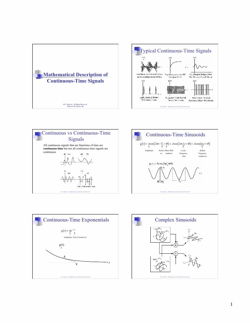
Typical Continuous-Time Signals
M. J. Roberts - All Rights Reserved. Edited by Dr. Robert Akl
Continuous vs Continuous-Time Signals
All continuous signals that are functions of time are continuous-time but not all continuous-time signals are continuous
M. J. Roberts - All Rights Reserved. Edited by Dr. Robert Akl
Continuous-Time Sinusoids
g t( ) = Acos 2πt / T0 +θ( ) = Acos 2π f0t +θ( ) = Acos ω0t +θ( ) ↑ ↑ ↑ ↑ ↑ Amplitude Period Phase Shift Cyclic Radian (s) (radians) Frequency Frequency (Hz) (radians/s)
M. J. Roberts - All Rights Reserved. Edited by Dr. Robert Akl
Continuous-Time Exponentials
g t( ) = Ae− t /τ ↑ ↑ Amplitude Time Constant (s)
M. J. Roberts - All Rights Reserved. Edited by Dr. Robert Akl
Complex Sinusoids
M. J. Roberts - All Rights Reserved. Edited by Dr. Robert Akl

2
The Signum Function
sgn t( ) = 1 , t > 0 0 , t = 0−1 , t < 0
⎧⎨⎪
⎩⎪
⎫⎬⎪
⎭⎪
Precise Graph Commonly-Used Graph
The signum function, in a sense, returns an indication of the sign of its argument.
M. J. Roberts - All Rights Reserved. Edited by Dr. Robert Akl
The Unit Step Function
u t( ) =1 , t > 01 / 2 , t = 00 , t < 0
⎧⎨⎪
⎩⎪
The product signal g t( )u t( ) can be thought of as the signal g t( )“turned on” at time t = 0.
M. J. Roberts - All Rights Reserved. Edited by Dr. Robert Akl
The Unit Step Function
The unit step function can mathematically describe a signal that is zero up to some point in time and non- zero after that.
v RC t( ) =Vb u t( )i t( ) = Vb / R( )e− t / RC u t( )vC t( ) =Vb 1− e− t / RC( )u t( )
M. J. Roberts - All Rights Reserved. Edited by Dr. Robert Akl
The Unit Ramp Function
ramp t( ) = t , t > 00 , t ≤ 0
⎧⎨⎩
⎫⎬⎭= u λ( )dλ
−∞
t
∫ = t u t( )
M. J. Roberts - All Rights Reserved. Edited by Dr. Robert Akl
The Unit Ramp Function
Product of a sine wave and a ramp function.
M. J. Roberts - All Rights Reserved. Edited by Dr. Robert Akl
Introduction to the Impulse
Define a function Δ t( ) = 1 / a , t < a / 20 , t > a / 2
⎧⎨⎩
Let another function g t( ) be finite and continuous at t = 0.
M. J. Roberts - All Rights Reserved. Edited by Dr. Robert Akl

3
Introduction to the Impulse The area under the product of the two functions is
A = 1a
g t( )dt−a /2
a /2
∫As the width of Δ t( ) approaches zero,
lima→0
A = g 0( ) lima→0
1a
dt−a /2
a /2
∫ = g 0( ) lima→0
1aa( ) = g 0( )
The continuous-time unit impulse is implicitly defined by
g 0( ) = δ t( )g t( )dt−∞
∞
∫
M. J. Roberts - All Rights Reserved. Edited by Dr. Robert Akl
The Unit Step and Unit Impulse As a approaches zero, g t( ) approaches a unitstep and ′g t( ) approaches a unit impulse.
The unit step is the integral of the unit impulse and the unit impulse is the generalized derivative of theunit step.
M. J. Roberts - All Rights Reserved. Edited by Dr. Robert Akl
Graphical Representation of the Impulse
The impulse is not a function in the ordinary sense because its value at the time of its occurrence is not defined. It is represented graphically by a vertical arrow. Its strength is either written beside it or is represented by its length.
M. J. Roberts - All Rights Reserved. Edited by Dr. Robert Akl
Properties of the Impulse The Sampling Property
g t( )δ t − t0( )dt−∞
∞
∫ = g t0( )The sampling property “extracts” the value of a function ata point.The Scaling Property
δ a t − t0( )( ) = 1aδ t − t0( )
This property illustrates that the impulse is different from ordinary mathematical functions.
M. J. Roberts - All Rights Reserved. Edited by Dr. Robert Akl
The Unit Periodic Impulse
The unit periodic impulse is defined by
δT t( ) = δ t − nT( )n=−∞
∞
∑ , n an integer
The periodic impulse is a sum of infinitely many uniformly-spaced impulses.
M. J. Roberts - All Rights Reserved. Edited by Dr. Robert Akl
The Periodic Impulse
M. J. Roberts - All Rights Reserved. Edited by Dr. Robert Akl

4
The Unit Rectangle Function
rect t( ) = 1 , t <1 / 21 / 2 , t = 1 / 2 0 , t >1 / 2
⎧
⎨⎪
⎩⎪
⎫
⎬⎪
⎭⎪= u t +1 / 2( )− u t −1 / 2( )
The product signal g t( )rect t( ) can be thought of as the signal g t( )“turned on” at time t = −1 / 2 and “turned back off” at time t = +1 / 2.
M. J. Roberts - All Rights Reserved. Edited by Dr. Robert Akl
Combinations of Functions
M. J. Roberts - All Rights Reserved. Edited by Dr. Robert Akl
Shifting and Scaling Functions Let a function be defined graphically by
and let g t( ) = 0 , t > 5
M. J. Roberts - All Rights Reserved. Edited by Dr. Robert Akl
Shifting and Scaling Functions Amplitude Scaling,
�
g t( )→ Ag t( )
M. J. Roberts - All Rights Reserved. Edited by Dr. Robert Akl
Shifting and Scaling Functions
Time shifting, t→ t − t0
M. J. Roberts - All Rights Reserved. Edited by Dr. Robert Akl
Shifting and Scaling Functions Time scaling, t→ t / a
M. J. Roberts - All Rights Reserved. Edited by Dr. Robert Akl
5
Shifting and Scaling Functions
Multiple transformations g t( )→ Ag t − t0a
⎛⎝⎜
⎞⎠⎟
A multiple transformation can be done in steps
g t( )amplitudescaling, A⎯ →⎯⎯⎯ Ag t( ) t→t /a⎯ →⎯⎯ Ag t
a⎛⎝⎜
⎞⎠⎟
t→t−t0⎯ →⎯⎯ Ag t − t0a
⎛⎝⎜
⎞⎠⎟
The sequence of the steps is significant
g t( )amplitudescaling, A⎯ →⎯⎯⎯ Ag t( ) t→t−t0⎯ →⎯⎯ Ag t − t0( ) t→t /a⎯ →⎯⎯ Ag t
a− t0
⎛⎝⎜
⎞⎠⎟ ≠ Ag t − t0
a⎛⎝⎜
⎞⎠⎟
M. J. Roberts - All Rights Reserved. Edited by Dr. Robert Akl
Shifting and Scaling Functions Simultaneous scaling and shifting g t( )→ Ag t − t0
a⎛⎝⎜
⎞⎠⎟
M. J. Roberts - All Rights Reserved. Edited by Dr. Robert Akl
Shifting and Scaling Functions
Simultaneous scaling and shifting, Ag bt − t0( )
M. J. Roberts - All Rights Reserved. Edited by Dr. Robert Akl
Shifting and Scaling Functions
M. J. Roberts - All Rights Reserved. Edited by Dr. Robert Akl
Shifting and Scaling Functions
If g2 t( ) = Ag1 t − t0( ) / w( ) what are A, t0 and w?
M. J. Roberts - All Rights Reserved. Edited by Dr. Robert Akl
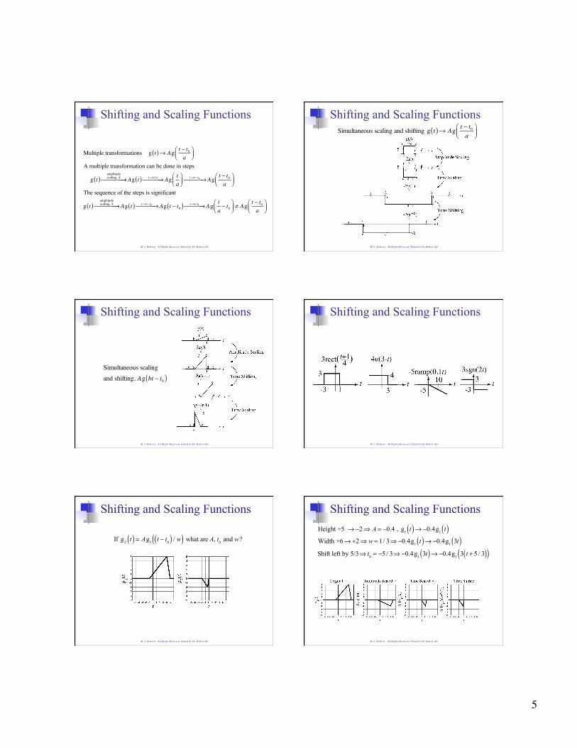
Shifting and Scaling Functions
Height +5 →−2⇒ A = −0.4 , g1 t( )→−0.4g1 t( )Width +6→ +2⇒ w = 1/ 3⇒−0.4g1 t( )→−0.4g1 3t( )Shift left by 5/3⇒ t0 = −5 / 3⇒−0.4g1 3t( )→−0.4g1 3 t + 5 / 3( )( )
M. J. Roberts - All Rights Reserved. Edited by Dr. Robert Akl

6
Shifting and Scaling Functions
If g2 t( ) = Ag1 wt − t0( ) what are A, t0 and w?
M. J. Roberts - All Rights Reserved. Edited by Dr. Robert Akl
Shifting and Scaling Functions
Height +5 →−2⇒ A = −0.4 ⇒ g1 t( )→−0.4g1 t( )Shift left 5⇒ t0 = −5⇒−0.4g1 t( )→−0.4g1 t + 5( )Width +6 to +2⇒ w = 3⇒−0.4g1 t + 5( )→−0.4g1 3t + 5( )
M. J. Roberts - All Rights Reserved. Edited by Dr. Robert Akl
Shifting and Scaling Functions
If g2 t( ) = Ag1 w t − t0( )( ) what are A, t0 and w?
M. J. Roberts - All Rights Reserved. Edited by Dr. Robert Akl
Shifting and Scaling Functions
Height +5 →−3⇒ A = −0.6⇒ g1 t( )→−0.6g1 t( )Width +6→−3⇒ w = −2⇒−0.6g1 t( )→−0.6g1 −2t( )Shift Right 1/2⇒ t0 = 1/ 2⇒−0.6g1 −2t( )→−0.6g1 −2 t −1/ 2( )( )
M. J. Roberts - All Rights Reserved. Edited by Dr. Robert Akl
Shifting and Scaling Functions
If g2 t( ) = Ag1 t / w− t0( ) what are A, t0 and w?
M. J. Roberts - All Rights Reserved. Edited by Dr. Robert Akl
Shifting and Scaling Functions
Height +5 →−3⇒ A = −0.6⇒ g1 t( )→−0.6g1 t( )Shift Left 1⇒ t0 = −1⇒−0.6g1 t( )→−0.6g1 t +1( )Width +6→−3⇒ w = −1/ 2⇒−0.6g1 t +1( )→−0.6g1 −2t +1( )
M. J. Roberts - All Rights Reserved. Edited by Dr. Robert Akl

7
Differentiation
M. J. Roberts - All Rights Reserved. Edited by Dr. Robert Akl
Integration
M. J. Roberts - All Rights Reserved. Edited by Dr. Robert Akl
Even and Odd Signals Even Functions Odd Functionsg t( ) = g −t( ) g t( ) = −g −t( )
M. J. Roberts - All Rights Reserved. Edited by Dr. Robert Akl
Even and Odd Parts of Functions
The even part of a function is ge t( ) = g t( ) + g −t( )2
.
The odd part of a function is go t( ) = g t( )− g −t( )2
.
A function whose even part is zero is odd and a functionwhose odd part is zero is even.The derivative of an even function is odd and the derivativeof an odd function is even.The integral of an even function is an odd function, plus aconstant, and the integral of an odd function is even.
M. J. Roberts - All Rights Reserved. Edited by Dr. Robert Akl
Even and Odd Parts of Functions
M. J. Roberts - All Rights Reserved. Edited by Dr. Robert Akl
Products of Even and Odd Functions
Two Even Functions
M. J. Roberts - All Rights Reserved. Edited by Dr. Robert Akl

8
Products of Even and Odd Functions An Even Function and an Odd Function
M. J. Roberts - All Rights Reserved. Edited by Dr. Robert Akl
Products of Even and Odd Functions An Even Function and an Odd Function
M. J. Roberts - All Rights Reserved. Edited by Dr. Robert Akl
Products of Even and Odd Functions Two Odd Functions
M. J. Roberts - All Rights Reserved. Edited by Dr. Robert Akl
g t( )dt−a
a
∫ = 2 g t( )dt0
a
∫ g t( )dt−a
a
∫ = 0
M. J. Roberts - All Rights Reserved. Edited by Dr. Robert Akl
Integrals of Even and Odd Functions
Integrals of Even and Odd Functions
M. J. Roberts - All Rights Reserved. Edited by Dr. Robert Akl
Periodic Signals
A function that is not periodic is aperiodic.
If a function g(t) is periodic, g t( ) = g t + nT( )where n is any integerand T is a period of the function. The minimum positive value of T for which g t( ) = g t +T( ) is called the fundamental period T0 of the function. The reciprocal of the fundamental period is the fundamental frequency f0 = 1 /T0 .
M. J. Roberts - All Rights Reserved. Edited by Dr. Robert Akl

9
Sums of Periodic Functions The period of the sum of periodic functions is the least common multiple of the periods of the individual functions summed. If the least common multiple is infinite, the sum function is aperiodic.
M. J. Roberts - All Rights Reserved. Edited by Dr. Robert Akl
ADC Waveforms
Examples of waveforms which may appear in analog-to-digital converters. They can be described by a periodic repetition of a ramp returned to zero by a negative step or by a periodic repetition of a triangle-shaped function.
M. J. Roberts - All Rights Reserved. Edited by Dr. Robert Akl
The signal energy of a signal x t( ) is
Ex = x t( ) 2 dt−∞
∞
∫
M. J. Roberts - All Rights Reserved. Edited by Dr. Robert Akl
Signal Energy and Power Signal Energy and Power
M. J. Roberts - All Rights Reserved. Edited by Dr. Robert Akl
Signal Energy and Power Find the signal energy of x t( ) = 2 rect t / 2( )− 4 rect t +1
4⎛⎝⎜
⎞⎠⎟
⎡⎣⎢
⎤⎦⎥
u t + 2( )
Ex = x t( ) 2 dt−∞
∞
∫ = 2 rect t / 2( )− 4 rect t +14
⎛⎝⎜
⎞⎠⎟
⎡⎣⎢
⎤⎦⎥
u t + 2( )2
dt−∞
∞
∫
Ex = 2 rect t / 2( )− 4 rect t +14
⎛⎝⎜
⎞⎠⎟
⎡⎣⎢
⎤⎦⎥
2
dt−2
∞
∫
Ex = 4 rect2 t / 2( ) +16 rect2 t +14
⎛⎝⎜
⎞⎠⎟ −16 rect t / 2( )rect t +1
4⎛⎝⎜
⎞⎠⎟
⎡⎣⎢
⎤⎦⎥dt
−2
∞
∫
Ex = 4 rect t / 2( )dt +16 rect t +14
⎛⎝⎜
⎞⎠⎟ dt
−2
∞
∫ −16 rect t / 2( )rect t +14
⎛⎝⎜
⎞⎠⎟
−2
∞
∫ dt−2
∞
∫
Ex = 4 dt +16 dt−2
1
∫ −16 dt−1
1
∫−1
1
∫ = 8 + 48 − 32 = 24
M. J. Roberts - All Rights Reserved. Edited by Dr. Robert Akl
Signal Energy and Power
Some signals have infinite signal energy. In that caseIt is more convenient to deal with average signal power.The average signal power of a signal x t( ) is
Px = limT→∞
1T
x t( ) 2 dt−T /2
T /2
∫For a periodic signal x t( ) the average signal power is
Px =1T
x t( ) 2 dtT∫
where T is any period of the signal.
M. J. Roberts - All Rights Reserved. Edited by Dr. Robert Akl

10
A signal with finite signal energy is called an energy signal. A signal with infinite signal energy and finite average signal power is called a power signal.
M. J. Roberts - All Rights Reserved. Edited by Dr. Robert Akl
Signal Energy and Power Find the average signal power of a signal x t( ) with fundamentalperiod 12, one period of which is described by x t( ) = ramp −t / 5( ) , − 4 < t < 8
Px =1T
x t( ) 2 dtT∫ = 1
12ramp −t / 5( ) 2 dt
−4
8
∫ = 112
−t / 5( )2 dt−4
0
∫
Px =1
12t 2
25dt
−4
0
∫ = 1300
t 3 / 3⎡⎣ ⎤⎦−4
0=
0 − −64 / 3( )300
= 16225
≅ 0.0711
M. J. Roberts - All Rights Reserved. Edited by Dr. Robert Akl
Signal Energy and Power