Lecture 4a: Continuous-Time Markov Chain Modelspeople.bu.edu/andasari/courses/stochasticmodeling/... · 2019-01-18 · Lecture 4a: Continuous-Time Markov Chain Models Continuous-time

Dr V. Andasari http://people.bu.edu/andasari/courses/stochasticmodeling/stochastics.html

Lecture 4a: Continuous-Time Markov Chain Models

Continuous-time Markov chains are stochastic processes whose time is continuous, t ∈[0,∞), but the random variables are discrete. Prominent examples of continuous-timeMarkov processes are Poisson and death and birth processes. These processes play afundamental role in the theory and applications that embrace queueing and inventorymodels, population growth, engineering systems, etc [3]. Here we discuss the Poissonprocess.

1 Preliminaries

Before discussing Poisson and death and birth processes, we review and take a look attheories and mathematical foundations needed to better understand this topic.

Please note that throughout this lecture, we use the notation Prob{·} in place of P{·} toemphasize that a probability is being computed, for example

P{X ≤ x} = Prob{X ≤ x} = F (x) , or P{X = x} = Prob{X = x} = f(x) .

1.1 The Exponential Distribution

In stochastic modeling, it is often assumed that certain random variables are exponentiallydistributed. The reason for this is that the exponential distribution is both relatively easyto work with and is often a good approximation to the actual distribution. One of theproperties of the exponential distribution is that it does not deteriorate with time. Itmeans that if the lifetime of an item is exponentially distributed, then an item that hasbeen in use for ten (or any number of) hours is as good as a new item in regards to theamount of time remaining until the item fails [7].

Let us consider a continuous random variable X. The random variable is said to have anexponential distribution with parameter λ with λ > 0, if its probability density function

1

http://people.bu.edu/andasari/courses/stochasticmodeling/stochastics.html


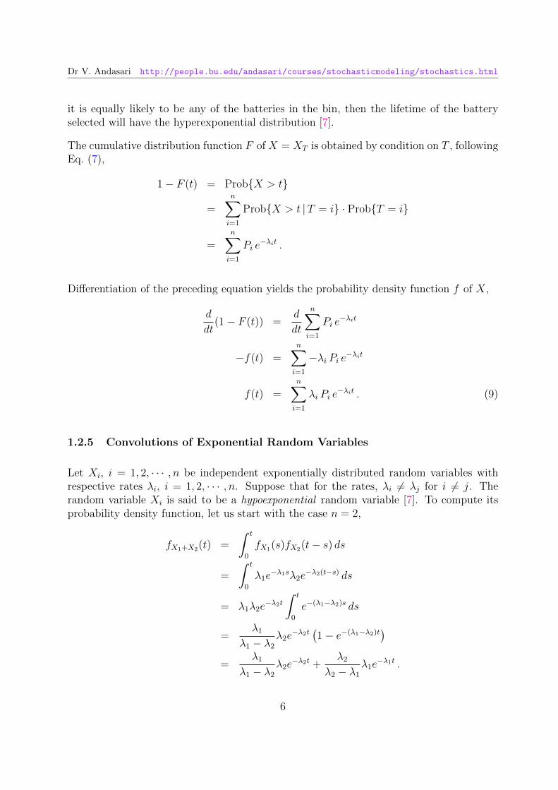
(p.d.f.) is given by

f(x) =

λ e−λx x ≥ 0

0 x < 0 ,

or, equivalently, if its cumulative distribution function (c.d.f.) is given by

F (x) =

∫ x

−∞f(y) dy =

1− e−λx x ≥ 0

0 x < 0 .

The expectation or mean of the exponential distribution, E[X] is given by

E[X] =

∫ ∞−∞

x f(x) dx

=

∫ ∞0

λx e−λx dx .

By letting u = x, dv = λ e−λx, and using these for integration by parts, we get

E[X] = −x e−λx∣∣∞0

+

∫ ∞0

e−λx dx =1

λ.

If X is exponentially distributed with mean 1/λ, then it can be shown (see its proof in thenext subsection) that

Prob{X > x} = e−λx .

The moment generating function (m.g.f.) of the exponential distribution is given by

φ(t) = E[etX ]

=

∫ ∞0

etx λ e−λx dx

=λ

λ− t, for t < λ . (1)

All the moments of X can be obtained by differentiating Eq. (1),

E[X2] =d2

dt2φ(t)

∣∣∣∣t=0

=2λ

(λ− t)3

∣∣∣∣t=0

=2

λ2, (2)

2



from which we obtain the variance,

Var(X) = E[X2]− (E[X])2

=2

λ2− 1

λ2

=1

λ2. (3)

1.2 Properties of the Exponential Distribution

1.2.1 Memoryless

The usefulness of exponential random variable derives from the fact that they possess thememoryless property [8], where a random variable X is said to be memoryless, or withoutmemory, if [7]:

Prob{X > s+ t |X > t} = Prob{X > s} ∀ s, t ≥ 0 . (4)

If we think of X as being the lifetime of some instrument, then Eq. (4) describes theprobability that the instrument lives for at least s + t hours given that it has survived thours is the same as the initial probability that it lives for at least s hours [7].

By definition of the conditional probability on the left hand side of Eq. (4), where

Prob{X > s+ t |X > t} =Prob{X > s+ t , X > t}

Prob{X > t}, (5)

and since Prob{X > s+t} is included in Prob{X > t}, the condition in Eq. (4) is equivalentto

Prob{X > s+ t |X > t} =Prob{X > s+ t}

Prob{X > t}=e−λ(s+t)

e−λt= e−λs = Prob{X > s} ,

orProb{X > s+ t} = Prob{X > s} · Prob{X > t} . (6)

Since Eq. (6) is satisfied when X is exponentially distributed, such as e−λ(s+t) = e−λse−λt,it follows that exponentially distributed random variables are memoryless [7].

1.2.2 Exponential Distribution

Aside from being memoryless, the exponential distribution is also the unique distributionpossessing the memoryless property. Let us assume that X is memoryless and

3



let F̄ (x) = Prob{X > x}. Then by Eq. (6), it follows that [7]

F̄ (s+ t) = F̄ (s) F̄ (t) .

That is, F̄ (x) satisfies the functional equation

g(s+ t) = g(s) g(t) .

However, the only solutions of the above equation that satisfy any sort of reasonablecondition (such as monotonicity, right or left continuity, or even measurability), are of theform [8]

g(x) = e−λx ,

which is the only right continuous solution, for some suitable value of λ. For proof of thissolution, see [7, 8]. Since a distribution function is always right continuous, we have

F̄ (x) = e−λx ,

orF (x) = Prob{X ≤ x} = 1− e−λx ,

which shows that the random variable X is exponentially distributed.

Alternatively,Prob{X > x} = 1− F (x) = e−λx . (7)

1.2.3 Gamma Distribution

Let X1, X2, · · · , Xn be independent and identically distributed exponential random vari-ables having mean 1/λ. Let us assume that X1 + X2 + · · · + Xn has density given by[7]

fX1+X2+···+Xn(t) =

∫ ∞0

fXn(t− s) fX1+X2+···+Xn−1(s) ds

=

∫ t

0

λ e−λ(t−s) λ e−λs(λs)n−2

(n− 2)!ds

= λ e−λt(λt)n−1

(n− 1)!,

for t ≥ 0, which shows a gamma distribution with parameters n and λ where λ > 0. Hencethe density for X1, X2, · · · , Xn−1 is given by [7]

fX1+X2+···+Xn−1(t) = λ e−λt(λt)n−2

(n− 2)!.

4



Another useful calculation is to determine the probability that one exponential randomvariable is smaller than another. Suppose that X1 and X2 are independent exponentialrandom variables with respective means 1/λ1 and 1/λ2. Then [7]

Prob{X1 < X2} =

∫ ∞0

Prob{X1 < X2 |X1 = x}λ1 e−λ1x dx

=

∫ ∞0

Prob{x < X2}λ1 e−λ1x dx

=

∫ ∞0

e−λ2x λ1 e−λ1x dx

=

∫ ∞0

λ1 e−(λ1+λ2)x dx

=λ1

λ1 + λ2

. (8)

Likewise,

Prob{X1 > X2} =λ2

λ1 + λ2

.

1.2.4 Hyperexponential Distribution

Suppose X1, X2, · · · , Xn are independent exponential random variables. If they are identi-cally distributed where the common mean is 1/λ, then the sum X1 +X2 + · · ·+Xn followsthe gamma distribution with shape parameter n and rate parameter λ.

If the exponential random variables X1, X2, · · · , Xn are not identically distributed, wherethe respective rates of the random variables are λ1, λ2, · · · , λn, or the rate parameter ofXi is λi, such that λi 6= λj for i 6= j, then the sum X1 + X2 + · · · + Xn is said to follow ahyperexponential distribution.

Let T be independent of these random variables and suppose that

n∑j=1

Pj = 1 , where Pj = Prob{T = j} .

The random variable XT is said to be a hyperexponential random variable. The hyperex-ponential distribution is the mixture of a set of independent exponential distributions. Tosee how such a random variable might originate, imagine that a bin contains n differenttypes of batteries, with a type j battery lasting for an exponential distributed time withrate λj, j = 1, 2, · · · , n. Suppose further that Pj is the proportion of batteries in the binthat are type j for each j = 1, 2, · · · , n. If a battery is randomly chosen, in the sense that

5



it is equally likely to be any of the batteries in the bin, then the lifetime of the batteryselected will have the hyperexponential distribution [7].

The cumulative distribution function F of X = XT is obtained by condition on T , followingEq. (7),

1− F (t) = Prob{X > t}

=n∑i=1

Prob{X > t |T = i} · Prob{T = i}

=n∑i=1

Pi e−λit .

Differentiation of the preceding equation yields the probability density function f of X,

d

dt(1− F (t)) =

d

dt

n∑i=1

Pi e−λit

−f(t) =n∑i=1

−λi Pi e−λit

f(t) =n∑i=1

λi Pi e−λit . (9)

1.2.5 Convolutions of Exponential Random Variables

Let Xi, i = 1, 2, · · · , n be independent exponentially distributed random variables withrespective rates λi, i = 1, 2, · · · , n. Suppose that for the rates, λi 6= λj for i 6= j. Therandom variable Xi is said to be a hypoexponential random variable [7]. To compute itsprobability density function, let us start with the case n = 2,

fX1+X2(t) =

∫ t

0

fX1(s)fX2(t− s) ds

=

∫ t

0

λ1e−λ1sλ2e

−λ2(t−s) ds

= λ1λ2e−λ2t

∫ t

0

e−(λ1−λ2)s ds

=λ1

λ1 − λ2

λ2e−λ2t

(1− e−(λ1−λ2)t

)=

λ1

λ1 − λ2

λ2e−λ2t +

λ2

λ2 − λ1

λ1e−λ1t .

6



For the case n = 3,

fX1+X2+X3(t) =

∫ t

0

fX3(t− s)fX1+X2(s) ds

=

∫ t

0

λ3e−λ3(t−s) λ1

λ1 − λ2

λ2e−λ2s

(1− e−(λ1−λ2)s

)ds

=λ1λ2λ3

λ1 − λ2

e−λ3t∫ t

0

e(λ3−λ2)s ds+λ1λ2λ3

λ2 − λ1

e−λ3t∫ t

0

e(λ3−λ1)s ds

=λ1λ2λ3

(λ1 − λ2)(λ3 − λ2)e−λ2t − λ1λ2λ3

(λ1 − λ2)(λ3 − λ2)e−λ3t +

λ1λ2λ3

(λ2 − λ1)(λ3 − λ1)e−λ1t − λ1λ2λ3

(λ2 − λ1)(λ3 − λ1)e−λ3t

=

(λ2

λ2 − λ1

)(λ3

λ3 − λ1

)λ1e

−λ1t +

(λ1

λ1 − λ2

)(λ3

λ3 − λ2

)λ2e

−λ2t

+

(λ1

λ1 − λ3

)(λ2

λ2 − λ3

)λ3e

−λ3t

=3∑i=1

λie−λit

(∏j 6=i

λjλj − λi

).

In general,

fX1+···+Xn(t) =n∑i=1

λie−λit

(∏j 6=i

λjλj − λi

).

If T =∑n

i=1Xi, then

fT (t) =n∑i=1

Ci,n λi e−λit , (10)

where

Ci,n =∏j 6=i

λjλj − λi

.

Integrating both sides of the expression for fT from t to ∞, see Eq. (9), yields the tail

7



distribution function of T , that is∫ ∞t

fT (s)ds =

∫ ∞t

n∑i=1

Ci,n λi e−λisds

1− F (t) =n∑i=1

Ci,ne−λit

Prob{T > t} =n∑i=1

Ci,n e−λit . (11)

1.3 The Law of Total Probability

In probability theory, the law (or formula) of total probability is a fundamental rule relatingmarginal probabilities to conditional probabilities [11]. The law states that:

Given n mutually exclusive events B1, B2, · · · , Bn whose probabilities sum toone, then for any event A we have

Prob(A) = Prob(A|B1) Prob(B1) + · · ·+ Prob(A|Bn) Prob(Bn)

where Prob(A|Bi) is the conditional probability.

Example 4a.1

Let X and Y be independent random variables having Poisson distributions with param-eters µ and ν, respectively. Calculate the distribution of the sum X + Y .

Solution:

Recall that the Poisson distribution with parameter λ > 0 is given by

Pk = Prob{X = k} =e−λλk

k!, for k = 0, 1, 2, · · · (12)

The sum X + Y has a Poisson distribution with parameter µ + ν. By the law of totalprobability,

Prob{X + Y = n} =n∑k=0

Prob{X = k, Y = n− k}

=n∑k=0

Prob{X = k}Prob{Y = n− k} ,

8



provided that X and Y are independent. Then

Prob{X + Y = n} =n∑k=0

(µke−µ

k!

)(νn−ke−ν

(n− k)!

)=

eµ+ν

n!

n∑k=0

n!

k!(n− k)!µkνn−k . (13)

The binomial expansion of (µ+ ν)n is

(µ+ ν)n =n∑k=0

n!

k!(n− k)!µkνn−k ,

so Eq. (13) simplifies to

Prob{X + Y = n} =e−(µ+ν)(µ+ ν)n

n!, n = 0, 1, 2, · · ·

the desired Poisson distribution. �

1.4 Negative Binomial Distribution

The negative binomial distribution is a discrete probability distribution. Assume Bernoullitrials, where:

(1) there are only two possible outcomes,

(2) each trial is independent,

(3) the number of trials is not fixed,

(4) the probability of success p for each trial is constant.

Let X denote the number of trials until the rth success occurs. Then, the probability massfunction of X is given by

f(x) = Prob{X = x} =

(x− 1

r − 1

)(1− p)x−rpr , (14)

for x = r, r+ 1, r+ 2, · · · . Hence we say that X follows a negative binomial distribution.

The negative binomial distribution is sometimes defined in terms of failure, e.g., the ran-dom variable Y = number of failures before rth success. This formulation is statistically

9



equivalent to the X = number of trials until the rth success occurs, by Y = X−r. Hence,the negative binomial can be expressed in its alternative form

Prob{Y = y} =

(r + y − 1

y

)(1− p)ypr , y = 0, 1, 2, · · · (15)

The moment generating function of a negative binomial random variable X is

M(t) = E[etX ] =(pet)r

(1− (1− p)et)r,

for (1− p)et < 1.

The mean of a negative binomial random variable X is

µ = E[X] =r

p.

The variance of a negative binomial random variable X is

σ2 = Var(x) =r(1− p)p2

.

1.5 Properties of the Continuous-Time Markov Chains

Let {X(t) : 0 ≤ t < ∞} be a collection of discrete random variables, where the possiblevalues of X(t) are the nonnegative integers in a finite, {0, 1, 2, · · · , N}, or infinite set,{0, 1, 2, · · · }. The index set is continuous, 0 ≤ t <∞.

Definition 1. The stochastic process {X(t) : 0 ≤ t < ∞} is called a continuous-timeMarkov chain if it satisfies the following condition:

For any sequence of real numbers satisfying 0 ≤ t0 < t1 < · · · < tn < tn+1,

Prob{X(tn+1) = in+1 |X(t0) = i0 , X(t1) = i1, · · · , X(tn) = in}= Prob{X(tn+1) = in+1 |X(tn) = in} .

(16)

This condition is known as the Markov property. The transition to the future state in+1

at time tn+1 depends only on the value of the current state in at the current time tn, doesnot depend on the past states. Each random variable X(t) has an associated probabilitydistribution {Pi(t)}∞i=0, where [1]

Pi(t) = Prob{X(t) = i} . (17)

10



We shall restrict our attention to the case where {X(t)} is a Markov process with stationarytransition probabilities, which is defined by

Pij(t) = Prob{X(t+ s) = j |X(s) = i} , (18)

for i, j = 0, 1, 2, · · · . The transition probability function in Eq. (47) states that a processpresently in state i will be in state j at time t − s later. These transition probabilitiesare called stationary or homogeneous transition probabilities if they depends only on thelength of the time interval t − s, not explicitly on t or s. Otherwise, they are referred toas non-stationary or non-homogeneous. The transition probabilities are stationary if

Pij(t− s) = Prob{X(t) = j |X(s) = i}= Prob{X(t− s) = j |X(0) = i} ,

for t > s.

Example 4a.2

Taken from [7]:

Suppose that a continuous-time Markov chain enters state i at some time, say, time 0, andsuppose that the process does not leave state i (or, a transition does not occur) during thenext ten minutes. What is the probability that the process will not leave state i duringthe following five minutes?

Solution:

Now since the process is in state i at time 10, it follows, by the Markov property, that theprobability that it remains in that state during the interval [10, 15] is just the (uncondi-tional) probability that it stays in state i for at least five minutes. That is, if we let Tidenote the amount of time that the process stays in state i before making a transition intoa different state, then

Prob{Ti > 15 |Ti > 10} = Prob{Ti > 5} ,

or, recall Eq. (4), in general,

Prob{Ti > s+ t |Ti > s} = Prob{Ti > t} , ∀ s, t ≥ 0 . �

The Markov property asserts that Pij(t) satisfies [3, 4, 9]

(a) The probabilities are positive:Pij(t) ≥ 0 .

11



(b) The sum of probabilities that there is a transition from state i to some other state(j) in time [0, t] equals one:

N∑j=0

Pij = 1 , i, j = 0, 1, 2, · · · .

(c) The transition probabilities Pij(t) are solutions of the Chapman-Kolmogorov equa-tions:

Pij(t+ s) =∞∑k=0

Pik(t)Pkj(s) , (19)

which states that in order to move from state i to state j in time t + s, X(t) movesto some state k in time t and then from state k to state j in the remaining time s.

(d) In addition, we postulate that

limt→0+

Pij(t) =

{1, i = j0, i 6= j .

If P(t) denotes the matrix of transition probabilities or the transition matrix, defined as

P(t) = (Pij(t)) , (20)

then property (c) or Eq. (19) can be written compactly in matrix notation as

P(t+ s) = P(t)P(s) , (21)

for all t ≥ 0, s ≥ 0.

These definitions are the continuous analogues of the definitions given for discrete-timeMarkov chains [1].

1.6 Limiting Probabilities

Here we present a theorem that enables us to calculate the limit limn→∞ P(n)ij by solving a

system of linear equations. The theorem in question is valid if the chain is irreducible andergodic, as defined below [6].

Consider state i of a Markov chain process that has period d, where P nii = 0 whenever n

is not divisible by d, and d is the largest integer. For example, starting in i, it may bepossible for the process to enter state i only at the times 2, 4, 6, 8, · · · . In this case, state ihas period 2. A state with period 1 is said to be aperiodic. State i is recurrent, if, startingin i the expected time until the process returns to state i is finite. Then state i is also saidto be positive recurrent. Positive recurrent, aperiodic states are called ergodic [7].

12



Theorem 1. The basic limit theorem of Markov chains

(a) Consider a recurrent, irreducible, aperiodic Markov chain. Let P(n)ii be the probability

of entering state i at the nth transition, n = 0, 1, 2, · · · , given that X0 = i (the initial

state is i), thus P(0)ii = 1. Let f

(n)ii be the probability of first returning to state i at the

nth transition, n = 0, 1, 2, · · · , where f(0)ii = 0. Then,

limn→∞

P(n)ii =

1∑∞n=0 nf

(n)ii

=1

mi

. (22)

(b) Under the same conditions as in (a),

limn→∞

P(n)ji = lim

n→∞P

(n)ii for all states j .

Theorem 2. For an irreducible, positive recurrent, and aperiodic (ergodic) Markov chain,

limn→∞ P(n)ij exists and is independent of i. Furthermore, letting

πj = limn→∞

P(n)ij , j ≥ 0 ,

then πj is the unique nonnegative solution of

πj =∞∑i=0

πiPij , for j ≥ 0 and∞∑j=0

πj = 1 , (23)

where π = (π0, π1, π2, · · · ) is a vector.

Example 4a.3

Taken from Example on pp. 173–174 in [10]:

Let the transition probability matrix of a Markov chain be

P =

[0.4 0.60.2 0.8

].

Computing successive powers of P gives

P(2) =

[0.28 0.720.24 0.76

]P(4) =

[0.2512 0.74880.2496 0.7504

]P(8) =

[0.25 0.750.25 0.75

]13



Note that the matrix P(8) is almost identical to the matrix P(4), and secondly, that each ofthe rows of P(8) has almost identical entries. In terms of matrix elements, it would seemthat P

(n)ij is converging to some value as n→∞, that is

limn→∞

P(n)ij = πj ,

which is the same for all i. Here, there seems to exist a limiting probability that the processwill be in state j after a large number of transitions, and this value is independent of theinitial state.

Equivalently,limn→∞

P(n) = P̂ .

Note that in general each row of P̂ has the same elements,

P̂ =

π0 π1 π2 · · ·π0 π1 π2 · · ·...

......

. . .

,

and that P̂ is a matrix whose rows are identical and equal to a vector

π = (π0, π1, π2, · · · ) . �

The vector π is called a stationary probability distribution.

For general cases, let us first define the following [9].

Definition 2. Suppose that a transition probability matrix P on a finite number of stateslabeled 0, 1, 2, · · · , N has the property that when raised to some power n, the matrix Pn hasall of its elements strictly positive. Such a transition probability matrix, or the correspond-ing Markov chain, is called regular.

Based on the preceding definition, we proceed to the following theorem [10].

Theorem 3. Let X = {X0, X1, X2, · · · } be a regular Markov chain with a finite numberN of states and transition probabilitty matrix P. Then

(i) Regardless of the value of i = 0, 1, 2, · · · , N ,

limn→∞

P(n)ij = πj > 0 , j = 0, 1, 2, · · · , N ,

14



(ii) or equivalently, in terms of the Markov chain {Xn},

limn→∞

Prob{Xn = j |X0 = i} = πj > 0 , j = 0, 1, 2, · · · , N ,

(iii) or equivalently, in matrix notation,

limn→∞

Pn = P̂

where P̂ is a matrix whose rows are identical and equal to the stationary probabilitydistribution vector

π = (π0, π1, π2, · · · , πN) .

(iv) The convergence means that, no matter in which state the chain begins at time 0 (or,regardless the initial probability distribution), the probability distribution approachesπ as n→∞.

(v) The stationary probability distribution π is the unique solution of

Pπ = π

satisfying π > 0 and∑

k πk = 1.

The limiting distribution is a stationary probability distribution if the continuous-timeMarkov chain is:

• positive recurrent,

• aperiodic, and

• irreducible.

Theorem 4. In a positive recurrent aperiodic class with states j = 0, 1, 2, · · · ,

limn→∞

P(n)ij = πj =

∞∑i=0

πiPij ,∞∑i=0

πi = 1 ,

and the π’s are uniquely determined by the set of equations

πi ≥ 0 ,∞∑i=0

πi = 1 , and πj =∞∑i=0

πiPij for j = 0, 1, 2, · · · (24)

15



Any set {πi}∞i=0 satisfying Eq. (24) is called a stationary probability distribution of theMarkov chain. A Markov chain that starts according to a stationary probability distribu-tion will follow this distribution at all points of time. Formally, if Prob{X0 = i} = π, thenProb{Xn = i} = πi for all n = 1, 2, · · · [9]. For example, for the case n = 1,

Prob{X1 = i} =∞∑k=0

Prob{X0 = k}Prob{X1 = i |X0 = k}

=∞∑k=0

πkPki

= πi .

Example 4a.4


Genes can be changed by certain stimuli, such as radiation. Sometimes in the ‘natural’course of events, chemical accidents may occur which change one allele to another. Suchalteration of genetic material is called mutation. Suppose that each A1 allele mutates to A2

with probability α1 per generation and that each A2 allele mutates to A1 with probabilityα2 per generation. By considering the ways in which a gene may be of type A1 we see that

Prob{a gene is A1 after mutation} = Prob{gene is A1 before mutation}× Prob{gene does not mutate from A1 to A2}+ Prob{gene is A2 before mutation}× Prob{gene mutates from A2 to A1} .

Thus, if there were j genes of type A1 in the parent population before mutation, theprobability pj of choosing an A1 gene when we form the next generation is

pj =j

2N(1− α1) +

(1− j

2N

)α2 . (25)

Let Xn be the number of A1 alleles at generation n. Suppose that there were j genes oftype A1 in generation n. We choose 2N genes to form generation n + 1 with probabilitypj of an A1 and probability 1− pj of an A2 at each trial. Then {Xn, n = 0, 1, 2, · · · } is atemporarily homogeneous Markov chain with one-step transition probabilities

Pjk = Prob{Xn+1 = k |Xn = j}

=

(2N

k

)pkj (1− pj)2N−k , j, k = 0, 1, 2, · · · , 2N, (26)

16



with p give by Eq. (25). Now if we let N = 1, α1 = α2 = 14, then substituting in Eq. (25),

pj =j

4+

1

4.

This gives p0 = 14, p1 = 1

2, p2 = 3

4. The elements of P are, for k = 0, 1, 2,

p0k =

(2

k

)(1

4

)k (3

4

)2−k

p1k =

(2

k

)(1

2

)2

p2k =

(2

k

)(3

4

)k (1

4

)2−k

,

obtained from Eq. (26). Evaluating these we get

P =1

16

9 6 14 8 41 6 9

.

All states of the Markov chain communicate with each other, thus there is one class andthe chain is irreducible. The chain has no absorbing states as there are no ones on theprincipal diagonal. All elements of P are non-zero, so at any time step a transition ispossible from any state to another.

Computing successive powers of P results in

limn→∞

Pn =

0.285 0.428 0.285

0.285 0.428 0.285

0.285 0.428 0.285

,

where the rows are identical and equal to

π = (0.285 0.428 0.285) ,

which is the stationary probability distribution.

We can also find π by solving Pπ = π, or

[π0 π1 π2

] 9 6 14 8 41 6 9

= 16[π0 π1 π2

]17



gives three equations, where the first two equations are

9π0 + 4π1 + π2 = 16π0

6π0 + 8π1 + 6π2 = 16π1

or

7π0 − 4π1 − π2 = 0

−6π0 + 8π1 − 6π2 = 0 .

Since of the components of π is arbitrary, setting π2 = 1 yields π0 = 1 and π1 = 32. The

sum of the components of π is 72, so dividing each element of π by 7

2gives us the required

stationary probability vector

π = (0.285 0.428 0.285) . �

Example 4a.5

Taken from Example on pp. 177–178 in [10], which shows that a stationary distri-bution may exist but it does not imply that a steady-state is approached as n→∞.

Consider a Markov chain with two states 0 and 1, that is

P =

[P00 P01

P10 P11

]=

[0 11 0

]

so that transitions are only possible from one state to the other. Solving

Pπ = π

or, [π0 π1

] [ 0 11 0

]=[π0 π1

]gives π0 = π1. If we set π0 = 1, then π1 = 1. Since the sum of the components (π0 + π1)is 2, so dividing each element of π by 2 we obtain the stationary probability distributionvector

π =

[1

2

1

2

].

18



However, as n→∞, Pn does not approach a constant matrix, because

Pn =

[0 11 0

], n = 1, 3, 5, · · ·

[1 00 1

], n = 2, 4, 6, · · ·

It can be seen that state 1 can only be entered from state 0 (P01 6= 0) and vice versa(P10 6= 0) on time steps 1, 3, 5, · · · . This Markov chain is not regular and periodic withperiod 2. Since state 0 and state 1 communicate with each other or 0 ↔ 1, then there isonly one class {0, 1} and the chain is irreducible. From the recurrence theory in Lecture3, we see that states 0 and 1 are recurrent, because

∞∑n=1

f(n)00 = P00 + P01 = 0 + 1 = 1 ,

and∞∑n=1

f(n)11 = P11 + P10 = 0 + 1 = 1 . �

If a Markov chain is reducible and/or periodic, then there can be many stationary distri-butions, as in the preceding example.

In addition to being the limiting probabilities, the πj’s also represent the proportion oftime that the process spends in state j, over a long period of time. That is, if the chainis positive recurrent but periodic, then this is the only interpretation of the πj’s [6]. Onaverage, the process spends one time unit in state j for µj time units, from which

πj =1

µj,

where

µj =∞∑n=1

n f(n)jj ,

which is the mean (average number) of transitions needed by the process, starting fromstate j, to return to j for the first time [6], or also known as first return probabilities (seeLecture 3).

19



1.7 Counting Process

Let {X(t) : t ≥ 0} be a stochastic process. If X(t) represents the total number of “events”that occur by time t, the stochastic process is said to be a counting process. Some examplesof counting processes are as follows [7]:

(1) In a store, an event occurs whenever a customer enters the store. If we let X(t)equal the total number of customers who enter the store at or prior to time t, then{X(t), t ≥ 0} is a counting process. However, if we let X(t) equal the number ofcustomers who are already in the store at time t, then {X(t), t ≥ 0} is not a countingprocess.

(2) If we say that an event occurs whenever a child is born, then {X(t), t ≥ 0} is acounting process when X(t) equals the total number of babies who were born bytime t.

(3) In a soccer/football game, an event occurs whenever a given soccer player scores agoal. If X(t) equals the number of goals that the soccer player scores by time t, then{X(t), t ≥ 0} is a counting process.

From its definition, a counting process X(t) must satisfy the following:

(i) X(t) ≥ 0.

(ii) X(t) is integer valued.

(iii) If s < t, then X(s) ≤ X(t).

(iv) For s < t, X(t)−X(s) equals the number of events that occur in the interval (s, t].

A counting process is said to possess:

� independent increments if the numbers of events that occur in disjoint time intervalsare independent. For example, in the customer arrival counting process of example(1), the number of events that occur by time t = 10, that is, X(10), must be inde-pendent of the number of events that occur between times t = 10 and t = 15, that is,X(15)−X(10). Also, the number of customers arriving during one time interval, e.g.,X(25)−X(20) does not affect the number arriving during a different time interval,e.g., X(15)−X(10).

Definition 3. Let {X(t), t ∈ [0,∞)} be a continuous-time random process. We saythat X(t) has independent increments if, for all 0 ≤ t1 < t2 < · · · < tn, the randomvariables

X(t2)−X(t1) , X(t3)−X(t2) , · · · , X(tn)−X(tn−1)

are independent [13].

20



� stationary increments if the distribution of the number of events that occur in anytime interval depends only on the length of the time interval. In other words, acounting process is said to have stationary increments if, for all t2 > t1 ≥ 0,

X(t2)−X(t1) has the same distribution as X(t2 − t1) .

2 The Poisson Process

One of the most important counting processes is the Poisson process.

Definition 4. The counting process {X(t), t ≥ 0} is said to be a Poisson process havingrate λ, where λ > 0, if [7],

(i) For t = 0, X(0) = 0.

(ii) The process has independent increments.

(iii) The number of events in any interval of length t is Poisson distributed with mean λt.That is, for all s, t ≥ 0:

Prob{X(t+ s)−X(s) = n} = e−λt(λt)n

n!, n = 0, 1, 2, · · · (27)

Related to the customer arrival counting process of example (1) above, we assume thefollowing about the rate at which customers arrive [5]:

(1) The number of customers arriving during one time interval does not affect the numberof customers arriving during a different time interval → independent increments

(2) The “average” rate at which customers arrive remains constant.

(3) Customers arrive one at a time.

The first assumption implies that for 0 ≤ t1 < t2 < t3 < · · · < tn, the random variablesX(t2)−X(t1), · · · , X(tn)−X(tn−1) are independent.

By the second assumption, with λ is the rate at which customers arrive, then the processhas stationary increments. In other words, on average we expect λt customers in time t,hence

E[X(t)] = λ t ,

which explains why λ is called the rate of the process.

21



The rate λ in a Poisson process X(t) is the proportionality constant in the probability ofan event occurring during an arbitrarily small interval [9].

In a small time interval [t, t + ∆t], we expect that customers arrive one at a time, and anew customer arrives with probability about λ∆t. Mathematically, this can be preciselyexplained from Eq. (27), with n = 1 and using the Maclaurin’s (or power) series for theexpansion of e−λ∆t,

Prob{X(t+ ∆t)−X(t) = 1} = e−λ∆t (λ∆t)

1!

= (λ∆t)

(1− λ∆t+

1

2λ2∆t2 − · · ·

)= λ∆t− λ2∆t2 +

1

2λ3∆t3 − · · ·

= λ∆t+ o(∆t) ,

where the terms with ∆tk, k ≥ 2 are very small and all very small terms are group togetherin the notation o(∆t). Note that the formula of Maclaurin’s series for the expansion off(∆t) = e−λ∆t around ∆t = 0 is given by

f(0) = f(0) + ∆tf ′(0) +∆t2

2!f ′′(0) +

∆t3

3!f ′′′(0) + · · ·

with f(0) = e0 = 1, f ′(0) = −λ, f ′′(0) = λ2, and so on.

If within the small time interval there is no new customers arrive, n = 0, then the proba-bility is mathematically explained as,

Prob{X(t+ ∆t)−X(t) = 0} = e−λ∆t (λ∆t)0

0!= e−λ∆t

= 1− λ∆t+1

2λ2∆t2 − · · ·

= 1− λ∆t+ o(∆t) .

The third assumption states that the probability that more than one customer arrivesduring a small time interval is significantly small. Mathematically, using Eq. (27) withn = 2, it also results in terms with ∆t2 and even smaller, hence the transition probabilityonly equals o(∆t),

Prob{X(t+ ∆t)−X(t) = 2} = e−λ∆t (λ∆t)2

2!

=1

2!(λ∆t)2

(1− λ∆t+

1

2λ2∆t2 − · · ·

)= o(∆t) .

22



Obviously, equations with n = 3, 4, · · · also result in only very small terms, hence it isappropriate to write the transition probabilities as

Prob{X(t+ ∆t)−X(t) ≥ 2} = o(∆t) .

All these lead to an alternate definition of a Poisson process for phenomena with infinites-imal probabilities.

Definition 5. The counting process {X(t), t ≥ 0} is said to be a Poisson process havingrate λ where λ > 0, if [7]

(i) For t = 0, X(0) = 0.

(ii) The process has stationary and independent increments.

(iii) For ∆t sufficiently small, the transition probabilities are [7]

Pii(∆t) = Prob{X(t+ ∆t)−X(t) = 0} = 1− λ∆t+ o(∆t) ,

Pi,i+1(∆t) = Prob{X(t+ ∆t)−X(t) = 1} = λ∆t+ o(∆t) ,

Pij(∆t) = Prob{X(t+ ∆t)−X(t) ≥ 2} = o(∆t) ,

(28)

where the notation o(∆t) represents some function that is much smaller than ∆t forsmall ∆t.

Another way of writing these transition probabilities is:

Pii(∆t) = Prob{X(t+ ∆t) = i |X(t) = i} = 1− λ∆t+ o(∆t) ,

Pi,i+1(∆t) = Prob{X(t+ ∆t) = i+ 1 |X(t) = i} = λ∆t+ o(∆t) ,

Pij(∆t) = Prob{X(t+ ∆t) = j |X(t) = i} = o(∆t) , if j ≥ i+ 2

Pij(∆t) = 0 , if j < i

(29)

The transition probabilities in Eq. (29) are obtained after using the conditional probabilitiesand making use of independent increments. For example,

Prob{X(t+ ∆t) = i |X(t) = i} =Prob{X(t+ ∆t) = i , X(t) = i}

Prob{X(t) = i}

= Prob{X(t+ ∆t) = i}

= Prob{X(t+ ∆t) = X(t)} , by the condition i = X(t)

= Prob{X(t+ ∆t)−X(t) = 0} .

23



Likewise, for the other two equations.

Definition 6. The function f(∆t) is said to be o(∆t), or f(∆t) = o(∆t), as ∆t→ 0 if

lim∆t→0

f(∆t)

∆t= lim

∆t→0

o(∆t)

∆t= 0 .

The following are examples and properties of o(∆t) [7]:

(i) The function f(x) = x2 is o(∆t) since

lim∆t→0

f(∆t)

∆t= lim

∆t→0

(∆t)2

∆t= lim

∆t→0∆t = 0

(ii) The function f(x) = x is not o(∆t) since

lim∆t→0

f(∆t)

∆t= lim

∆t→0

∆t

∆t= lim

∆t→01 = 1 6= 0

(iii) If f(·) is o(∆t) and g(·) is o(∆t), then so is f(·) + g(·), since

lim∆t→0

f(∆t) + g(∆t)

∆t= lim

∆t→0

f(∆t)

∆t+ lim

∆t→0

g(∆t)

∆t= 0 + 0 = 0

(iv) If f(·) is o(∆t), then so is g(·) = c f(·), since

lim∆t→0

c f(∆t)

∆t= c lim

∆t→0

f(∆t)

∆t= c · 0 = 0

(v) From (iii) and (iv), it follows that any finite linear combination of functions, each ofwhich is o(∆t), is o(∆t).

The transition probabilities in Eq. (28) are o(∆t) as ∆t→ 0, in particular

lim∆t→0

Pi,i+1(∆t)− λ∆t

∆t= lim

∆t→0

o(∆t)

∆t= 0

lim∆t→0

Pii(∆t)− 1 + λ∆t

∆t= lim

∆t→0

o(∆t)

∆t= 0

lim∆t→0

Pij(∆t)

∆t= lim

∆t→0

o(∆t)

∆t= 0 , j ≥ i+ 2 .

In order for the function f(·) to be o(∆t), it is necessary that f(∆t)∆t

go to zero as ∆t goes

to zero. But if ∆t goes to zero, the only way for f(∆t)∆t

to go to zero is for f(∆t) to go to

24



zero faster than ∆t does. That is, for ∆t small, f(∆t) must be small compared with ∆t[7].

In a small time interval ∆t, the Poisson process can either stay in the same state ormove to the next larger state, i → i + 1; it cannot move to a smaller state. Note thatthe transition probabilities Pij(∆t) are independent of i and j and only depend on thelength of the interval ∆t, see Eq. (28). For the Poisson process to have independent andstationary increments, the intervals [s, s+∆t] and [t, t+∆t] must be non-overlapping, thatis s + ∆t ≤ t. Then these random variables from the Poisson process, X(t + ∆t) − X(t)and X(s + ∆t)−X(s) are independent and have the same probability distributions (i.e.,the Poisson process has stationary and independent increments) [1].

Now we derive a system of differential equations for Pi(t) for i = 0, 1, 2, · · · . Note that inthe Poisson process X(0) = 0:

• For i = 0:From the definition of a probability distribution in Eq. (17), that is

Pi(t) = Prob{X(t) = i}

thenP0(t+ ∆t) = Prob{X(t+ ∆t) = 0}

and byX(t+ ∆t) = X(t)−X(0) +X(t+ ∆t)−X(t)

where X(t) − X(0) = X(t) and X(t + ∆t) − X(t) are independent, and if we letP00(t+ ∆t) = P0(t+ ∆t), by the law of total probability

P0(t+ ∆t) = Prob{X(t+ ∆t) = 0}= Prob{X(t) = 0, X(t+ ∆t)−X(t) = 0}= Prob{X(t) = 0} · Prob{X(t+ ∆t)−X(t) = 0}= Prob{X(t) = 0} · Prob{X(∆t) = 0} . (30)

Due to Pi(t) = Prob{X(t) = i}, then Eq. (30) becomes

P0(t+ ∆t) = P0(t) · P0(∆t) . (31)

Since

P0(∆t) = Prob{X(∆t) = 0}= Prob{X(t+ ∆t)−X(t) = 0}= Prob{X(t+ ∆t) = X(t)}= 1− λ∆t+ o(∆t) ,

25



which, after being substituted into Eq. (31)

P0(t+ ∆t) = P0(t)[1− λ∆t+ o(∆t)

].

Subtracting P0(t) from both sides of the equation and dividing by ∆t yields

P0(t+ ∆t)− P0(t)

∆t= −λP0(t) + P0(t)

o(∆t)

∆t.

Taking the limit as ∆t→ 0,

lim∆t→0

P0(t+ ∆t)− P0(t)

∆t= − lim

∆t→0λP0(t) + lim

∆t→0P0(t)

o(∆t)

∆t︸︷︷︸= 0

,

gives us the following first-order linear differential equation for i = 0:

dP0(t)

dt= −λP0(t) . (32)

The general solution of the differential equation is

P0(t) = c0 e−λt ,

where c0 is a constant determined from the equation’s initial condition.

Given the initial condition P0(0) = Prob{X(0) = 0} = 1, the particular solution ofthe differential equation is

P0(t) = e−λt .

• For i ≥ 1:Similarly, by the law of total probability,

Pi(t+ ∆t) = Prob{X(t+ ∆t) = i}= Prob{X(t) = i, X(t+ ∆t)−X(t) = 0}

+ Prob{X(t) = i− 1, X(t+ ∆t)−X(t) = 1}+ Prob{X(t+ ∆t) = i, X(t+ ∆t)−X(t) ≥ 2} .

However, by the last definition of Eq. (28), the last term on the right hand side iso(∆t), since

Prob{X(t+ ∆t) = i,X(t+ ∆t)−X(t) ≥ 2} = Prob{X(t+ ∆t) = i} ·Prob{X(t+ ∆t)−X(t) ≥ 2}

= Prob{X(t+ ∆t) = i} · o(∆t)= Pi(t+ ∆t) · o(∆t)= o(∆t)

26



Applying the definition of the transition probabilities of Eq. (28) and the indepen-dence of the increments,

Pi(t+ ∆t) = Prob{X(t) = i} · Prob{X(t+ ∆t)−X(t) = 0}+

Prob{X(t) = i− 1} · Prob{X(t+ ∆t)−X(t) = 1}+ o(∆t)

= Pi(t) · P0(∆t) + Pi−1(t) · Pi,i+1(∆t) + o(∆t)

= Pi(t)[1− λ∆t+ o(∆t)

]+Pi−1(t)

[λ∆t+ o(∆t)

]+o(∆t)

Rearranging

Pi(t+ ∆t)− Pi(t) = −λ∆tPi(t) + λ∆tPi−1(t) + o(∆t)

where all terms with a factor of o(∆t) are put in the o(∆t) expression, and dividingboth sides by ∆t leads to

Pi(t+ ∆t)− Pi(t)∆t

= −λPi(t) + λPi−1(t) +o(∆t)

∆t.

Taking the limit as ∆t → 0 gives us the following system of difference-differentialequations for i ≥ 1:

dPi(t)

dt= −λPi(t) + λPi−1(t) . (33)

where, difference equations in the variable i and differential equations in the variablet.

If we multiply both sides of Eq. (33) by eλt (known as an integrating factor) andequate Pi(t) terms to the left, we get

eλt(dPi(t)

dt+ λPi(t)

)= λ eλt Pi−1(t) ,

which is equivalent tod

dt

(eλt Pi(t)

)= λ eλt Pi−1(t) .

Now if i = 1, using the solution P0(t) = e−λt for i = 0 above, we get

d

dt

(eλt P1(t)

)= λ .

Integrating both sides from 0 to t, yields the general solution

P1(t) = e−λt(λt+ c) .

27



Applying the initial conditions Pi(0) = 0 for i ≥ 1 gives c = 0, and thus the particularsolution is

P1(t) = λte−λt .

Next for i = 2, the differential equation is

dP2(t)

dt= −λP2(t) + λP1(t) = −λP2(t) + λ2te−λt

with the initial condition P2(0) = 0. Applying the same technique to P2(t) as forP1(t) yields the solution

P2(t) = (λt)2 e−λt

2!.

By induction, it can be shown that

Pi(t) = e−λt(λt)i

i!, i = 0, 1, 2, · · · (34)

Thus, Definition 5 implies Definition 4.

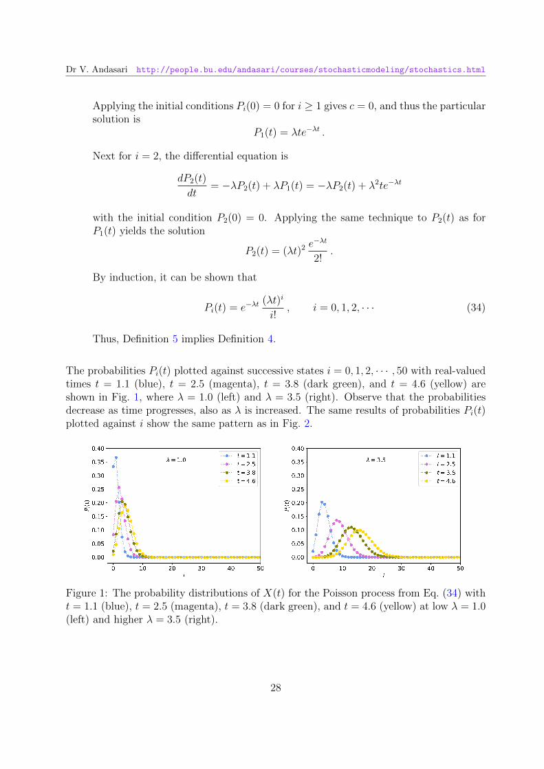
The probabilities Pi(t) plotted against successive states i = 0, 1, 2, · · · , 50 with real-valuedtimes t = 1.1 (blue), t = 2.5 (magenta), t = 3.8 (dark green), and t = 4.6 (yellow) areshown in Fig. 1, where λ = 1.0 (left) and λ = 3.5 (right). Observe that the probabilitiesdecrease as time progresses, also as λ is increased. The same results of probabilities Pi(t)plotted against i show the same pattern as in Fig. 2.

Figure 1: The probability distributions of X(t) for the Poisson process from Eq. (34) witht = 1.1 (blue), t = 2.5 (magenta), t = 3.8 (dark green), and t = 4.6 (yellow) at low λ = 1.0(left) and higher λ = 3.5 (right).

28



Figure 2: The probability distributions of X(t) for the Poisson process from Eq. (34) withλ = 0.1 (blue), λ = 0.5 (magenta), λ = 1.0 (dark green), and λ = 2.0 (yellow) at t = 5(left), t = 10 (middle), and t = 20 (right).

2.1 The Poisson Point Process

The Poisson point process is the simplest and most ubiquitous example of a point process.This process often arises in a form where the time parameter is replaced by a suitablespatial parameter. The Poisson point process is also said to be a spatial generalization ofthe Poisson process. A Poisson (counting) process on the line can be characterized by twoproperties: the number of points (or events) in disjoint intervals are independent and ithas a Poisson distribution [12].

Consider events occurring along the positive axis [0,∞), as shown in Fig. 3.

Figure 3: A Poisson point process.

Let N((a, b]) denote the number of events that occur during the interval (a, b]. That is,if t1 < t2 < t3 < · · · denote the times (or locations, etc.) of successive events, thenN((a, b]) is the number of values ti for which a < ti ≤ b. In other words, the N((a, b]) isa Poisson point process that counts the number of events occurring in an interval (a, b].A Poisson process X(t) counts the number of events occurring up to time t, or formallyX(t) = N((0, t]).

Definition 7. Let N((s, t]) be a random variable counting the number of events occurringin an interval (s, t]. Then N((s, t]) is a Poisson point process of intensity λ > 0 if

29



(i) for every m = 2, 3, · · · and distinct time points t0 = 0 < t1 < t2 < · · · < tm, therandom variables

N((t0, t1]), N((t1, t2]), · · · N((tm−1, tm])

are independent,

(ii) for any times s < t, the random variable N((s, t]) has the Poisson distribution

Prob{N((s, t]) = k} =(λ(t− s))k e−λ(t−s)

k!, k = 0, 1, 2, · · ·

2.2 Interevent and Waiting Time Distributions

Another way to view the Poisson process is to consider the waiting times between cus-tomers. Let Ti denote the time between the arrivals of the (i− 1)st and the ith customers,or the elapsed time between the (i−1)st and the ith events. The sequence {Ti, i = 1, 2, · · · }is called the sequence of the interevent times or sojourn times or holding times. For exam-ple, if T1 = 5 and T2 = 10, then the first event of the Poisson process would have occurredat time 5 and the second event at time 15 [7].

The fundamental difference between a discrete-time Markov chain and a continuous-timeMarkov chain is that in discrete-time Markov chains, there is a “jump” to a new state atdiscrete times 1, 2, · · · , but in continuous-time Markov chains, the “jump” to a new statemay occur at any real-valued time t ≥ 0 [1]. In a continuous-time chain, beginning at stateX(0), the process stays in state X(0) for a random amount of time W1 until it jumps toa new state, X(W1). Then it stays in state X(W1) for a random amount of time until itjumps to a new state at time W2, X(W2), and so on. In general, Wi is the random variablefor the time of the ith jump [1].

Fig. 4 shows a typical sample path of a Poisson process, where the random variable Wi isreferred to as the time of occurrence of the ith event, or the so-called jump time or waitingtime of the process. It is often convenient to set W0 = 0. The differences Ti = Wi+1 −Wi

are the ones that are referred to as the interevent/holding/sojourn times. The randomvariable Ti measures the duration that the Poisson process sojourns in state i.

The random variables Ti should be independent and identically distributed. The Ti shouldalso satisfy the loss of memory property, that is, if we have waited s time units for acustomer and no one has arrived, the chance that a customer will come in the next t timeunits is exactly the same as if there had been some customers before [5]. Mathematically,the property is written

Prob{Ti ≥ s+ t |Ti ≥ s} = Prob{Ti ≥ t} .

30



Figure 4: Sample path of a continuous-time Markov chain, illustrating waiting times (W1,W2, W3, and W4) and interevent/sojourn times (T0, T1, T2, and T3).

It is due to this memoryless property that Markov processes have an interevent/sojourntime Ti that is exponential.

To determine the distribution of the Ti, we note that the event {T1 > t} takes place ifand only if no events of the Poisson process occur in the interval [0, t], where T1 denotesthe random variable for the time until the process reaches state 1, or the time of the firstevent, which is the holding time until the first jump. Thus [1],

Prob{T1 > t} = Prob{X(t) = 0} = e−λt .

Alternatively,F (t) = Prob{T1 ≤ t} = 1− e−λt ,

which is the cumulative distribution function for an exponential random variable withparameter λ. Hence, T1 is an exponential random variable with parameter λ and havingan exponential distribution with mean 1/λ, with:

� Cumulative distribution function F (t) = 1− e−λt, and

� Probability distribution function f(t) =dF (t)

dt= λe−λt.

Now, for i = 2, to obtain the distribution of T2 condition on T1,

Prob{T2 > t |T1 = s} = Prob{0 events in (s, s+ t] |T1 = s}= Prob{0 events in (s, s+ t]} (by independent increments)

= e−λt (by stationary increments) (35)

31



where the last two equations follow from independent and stationary increments. Thus, T2

is also an exponential random variable with parameter λ, and T2 is independent of T1. Ingeneral, Ti, i = 1, 2, · · · are independent and identically distributed exponential randomvariables with parameter λ and mean 1/λ [7, 8]. In other words, it takes an exponentialamount of time to move from state i to state i + 1, or, the random variable for the timebetween jumps i and i + 1, Wi+1 −Wi, has an exponential distribution with parameterλ. In fact, sometimes in the definition of the Poisson process it is stated that the sojourntimes, Ti = Wi+1 −Wi, are independent exponential random variables with parameter λ[1].

In general, we have the following theorem [9]

Theorem 5. The sojourn/interevent/holding times T0, T1, · · · , Tn−1 are independent ran-dom variables, each having the exponential probability density function

fTk(t) = λe−λt , t ≥ 0 .

Proof. We need to show that the joint probability density function of T0, T1, · · · , Tn−1 isthe product of the exponential densities given by

fT0,T1,··· ,Tn−1(t0, t1, · · · , tn−1) = (λe−λt0)(λe−λt1) · · · (λe−λtn−1) . (36)

Because the general case is entirely similar, here we only give the proof for the case n = 2.Referring to Fig. 5, the joint occurrence of

t1 < T1 < t1 + ∆t1 and t2 < T2 < t2 + ∆t2

corresponds to no events in the intervals (0, t1] and (t1 +∆t1, t1 +∆t1 +t2], and exactly oneevent occurs in each of the intervals (t1, t1 + ∆t1] and (t1 + ∆t1 + t2, t1 + ∆t1 + t2 + ∆t2].From its definition, the Poisson process X(t) counts the number of events occurring up totime t, formally X(t) = N((0, t]). Thus

fT1,T2(t1, t2)∆t1∆t2 = Prob{t1 < T1 < t1 + ∆t1, t2 < T2 < t2 + ∆t2}+ o(∆t1∆t2)

= Prob{X(t1) = 0} × Prob{X(t2) = 0} × Prob{X(∆t1) = 1}× Prob{X(∆t2) = 1}+ o(∆t1∆t2)

= e−λt1e−λt2e−λ∆t1e−λ∆t2λ(∆t1)λ(∆t2) + o(∆t1∆t2)

= (λe−λt1)(λe−λt2)(∆t1)(∆t2) + o(∆t1∆t2)

whereX(t1) = N((0, t1]) ,X(t2) = N((t1 + ∆t1, t1 + ∆t1 + t2]) ,X(∆t1) = N((t1, t1 + ∆t1]) ,X(∆t2) = N((t1 + ∆t1 + t2, t1 + ∆t1 + t2 + ∆t2]) .

32



Dividing both sides by ∆t1∆t2 and taking the limits as ∆t1 → 0 and ∆t2 → 0, we obtain

fT1,T2(t1, t2) = (λe−λt1)(λe−λt2)

which is Eq. (36) in the case n = 2.

Figure 5:

Let Wi, i = 1, 2, · · · be the arrival time of the ith event, also referred to as the waitingtime until the ith event. We can see that

Wi =i∑

k=1

Tk , i ≥ 1 .

Theorem 6. The waiting time Wi has the gamma distribution whose probability densityfunction is

fWi(t) =

λiti−1

(i− 1)!e−λt , i = 1, 2, · · · , t ≥ 0 . (37)

In particular, W1, the time to the first event, is exponentially distributed,

fW1(t) = λe−λt , t ≥ 0 . (38)

Proof. The event Wi ≤ t occurs if and only if there are at least i events in the interval(0, t]. Since the number of events in (0, t] has a Poisson distribution with mean λt, weobtain the cumulative distribution function (c.d.f.) of Wn by

FWi(t) = Prob{Wi ≤ t} = Prob{X(t) ≥ i}

=∞∑k=i

(λt)ke−λt

k!

= 1−i−1∑k=0

(λt)ke−λt

k!, i = 1, 2, · · · , t ≥ 0 .

33



The probability distribution function (p.d.f.) is obtained by differentiating the c.d.f.FWi

(t), that is

fWi(t) =

d

dtFWi

(t)

=d

dt

(1− e−λt

(1− λt

1!+

(λt)2

2!− · · ·+ (λt)i−1

(i− 1)!

))= −e−λt

(λ+ λ

λt

1!+ λ

(λt)2

2!+ · · ·+ λ

(λt)i−2

(i− 2)!

)+ λe−λt

(1 +

λt

1!+

(λt)2

2!+ · · ·+ (λt)i−1

(i− 1)!

)=

λiti−1

(i− 1)!e−λt , i = 1, 2, · · · , t ≥ 0 .

Next, it is shown that the random variable Ti can be expressed in terms of the cumulativedistribution function (c.d.f.) Fi(t) and a uniform random variable U . This relationship isvery useful for computational purposes [1].

Theorem 7. Let U be a uniform random variable defined on [0, 1] and T be a contin-uous random variable defined on [0,∞). Then T = F−1(U), where F is the cumulativedistribution of the random variable T .

Proof. Since Prob{T ≤ t} = F (t), we want to show that Prob{F−1(U) ≤ t} = F (t). Firstnote that F : [0,∞) → [0, 1) is strictly increasing, so that F−1 exists. In addition, fort ∈ [0,∞),

Prob{F−1(U) ≤ t} = Prob{F (F−1(U)) ≤ F (t)}= Prob{U ≤ F (t)} .

Because U is a uniform random variable, then Prob{U ≤ y} = y for y ∈ [0, 1]. Thus,Prob{U ≤ F (t)} = F (t).

In the Poisson process, the only change in state is a birth that occurs with probabilityλ∆t + o(∆t) in a small interval of time ∆t. The cumulative distribution function for thesojourn/interevent time is

Fi(t) = Prob{Ti ≤ t} = 1− e−λt .

34



But because λ is independent of the state of the process, the sojourn/interevent time is thesame for every jump i, thus Ti ≡ T . The sojourn/interevent time T , expressed in terms ofthe uniform random variable U , is T = F−1(U). The function F−1(U) is found by solving

F (T ) = 1− e−λT = U

to get

T = − ln(1− U)

λ= F−1(U) .

However, because U is a uniform random variable on [0, 1], so is 1 − U . It follows thatthe sojourn/interevent time can be expressed in terms of a uniform random variable U asfollows

T = − ln(U)

λ. (39)

where U is a uniform random variable on [0, 1]. An example of Poisson process plot usingPython is shown in Fig. 6. The Python code for this figure is provided in the PythonImplementation section.

Figure 6: A sample path of a Poisson process with λ = 0.5 and 10 events.

For more general processes, the formula given in Eq. (39) for the sojourn/interevent timedepends on the state of the process.

The formula given in Eq. (39) for the sojourn/interevent time is applied to three simplebirth and death processes, known as simple birth process (or Yule process), simple deathprocess (or linear death process), and simple birth and death process. In each of theseprocesses, probabilities of births and deaths are linear functions of the population size. Inall cases, X(t) is the random variable for the total population size at time t.

35



2.3 Transition Rates and Infinitesimal Generator Matrix

In continuous-time Markov chains, the corresponding key quantities are the transitionrates, denoted by qij. The transition probabilities Pij are used to derive transition rates qij.The transition rates are used to define the forward and backward Kolmogorov differentialequations, which we discuss in the next section on birth and death processes.

Recall the four properties of the transition probabilities Pij(t) given in subsection 1.5 onproperties of the continuous-time Markov chains, rewrite here:

(a) Pij(t) ≥ 0 ,

(b)N∑j=0

Pij = 1 , i, j = 0, 1, 2, · · · ,

(c) The transition probabilities Pij(t) are solutions of the Chapman-Kolmogorov equa-tions:

Pij(t+ s) =∞∑k=0

Pik(t)Pkj(s) ,

or in the matrix form

P(t+ s) = P(t)P(s) , t, s ≥ 0 . (40)

(d) In addition, we postulate that

limt→0+

Pij(t) =

1, i = j

0, i 6= j .

Property (d) asserts that Pij(t) are continuous and differentiable for t ≥ 0, and at t = 0:

Pij(0) = Prob{X(s) = j |X(s) = i}

=

1, i = j

0, i 6= j

or

• Pij(0) = 0, for i 6= j.

• Pii(0) = 1.

In the matrix form, it leads to P(0) = I, where I is the identity matrix. Hence, P(t) iscontinuous at t = 0. It follows from Eq. (40) that P(t) is continuous for all t > 0:

36



♠ If s = h > 0, then due to the property (d), we have [3, 4, 9]

limh→0+

P(t+ h) = P(t) limh→0+

P(h) = P(t) I = P(t) . (41)

♠ Whereas when t > 0 and 0 < h < t, then

P(t) = P(t− h) P(h) . (42)

♠ But when s = ∆t and ∆t is sufficiently small, P(∆t) is near the identity and somatrix P(∆t) is invertible, or (P(∆t))−1 exists, and also approaches the identity I.Therefore [3, 4, 9]

P(t) = P(t) lim∆t→0+

(P(∆t))−1 = lim∆t→0+

P(t−∆t) . (43)

Now we look at the transition rates. For any pair of states i and j, the rate of the process,when in state i, makes a transition into state j, denoted by qij, is defined by [7]

qij = viPij ,

where vi is the rate at which the process makes a transition when in state i and Pijis the probability that this transition is into state j. The quantities qij are called theinstantaneous transition rates, and qij ≥ 0.

We can obtain vi fromvi = vi

∑j

Pij =∑j

viPij =∑j

qij .

Thus, the transition probabilities can be written as

Pij =qijvi

=qij∑j qij

.

Hence, specifying the instantaneous transition rates qij determines the parameters of thecontinuous-time Markov chain.

The rates qij and vi furnish an infinitesimal description of the process with [9]

Pii(∆t) = Prob{X(t+ ∆t) = i |X(t) = i} = 1− vi∆t+ o(∆t) ,

Pij(∆t) = Prob{X(t+ ∆t) = j |X(t) = i} = qij∆t+ o(∆t) , for i 6= j(44)

The limit relations in Eqs. (41) and (43) together show that Pij(t) are continuous. Theo-rems 1.1 and 1.2 in [4] (pp. 139–142) show that Pij(t) are differentiable with right-handderivatives. We use it to define the following:

37



(1) The probability that a process in state i at time 0 will not be in state i at time ∆t,which is 1 − Pii(∆t), equals the probability that a transition occurs within time ∆tplus something small compared to ∆t [7]. Hence,

1− Pii(∆t) = vi∆t+ o(∆t) , (45)

and dividing by ∆t and taking the limit as ∆t→ 0+ give us

lim∆t→0

1− Pii(∆t)∆t

= vi , ∀ i . (46)

(2) The probability that the process goes from state i to state j in a time ∆t, which isPij(∆t), equals the probability that a transition occurs in this time multiplied by theprobability that the transition is into state j, plus something small compared to ∆t[7]. That is,

Pij(∆t) = viPij∆t+ o(∆t) = qij∆t+ o(∆t) (47)

thus, the limit,

lim∆t→0

Pij(∆t)

∆t= qij , ∀ i, j; i 6= j . (48)

Note that since the amount of time until a transition occurs is exponentially distributed itfollows that the probability of two or more transitions in a time ∆t is o(∆).

From Eqs. (45) and (47), it follows that

Pij(∆t) = δij + qij∆t+ o(∆t) , (49)

where

δij =

0 if i 6= j

1 if i = j

and

qii = lim∆t→0+

Pii(∆t)− Pii(0)

∆t= lim

∆t→0

Pii(∆t)− 1

∆t(50)

= lim∆t→0+

−∑∞

j=0,j 6=i(qij∆t+ o(∆t))

∆t

= −∞∑

j=0,j 6=i

qij

= −vi . (51)

38



The transition rates qij and qii form a matrix known as the infinitesimal generator matrix Q.Matrix Q defines a relationship between the rates of change of the transition probabilities[1].

Individual limits in Eqs. (46) and (48) can be expressed more as the entries in a matrixlimit. Recall the matrix of transition probabilities defined in Eq. (20), and now we define

P(∆t) = (Pij(∆t)) (52)

as the infinitesimal transition matrix. Let I be the identity matrix having the same dimen-sion as P(∆t). Then matrix Q is defined as the one-sided derivative [1, 9]

Q = lim∆t→0+

P(∆t)− I

∆t, (53)

which shows that Q is the matrix derivative of P(t) at t = 0. Formally, Q = P′(0).

The matrix Q = (qij) is called the matrix of transition rates and whose elements are

Q =

q00 q01 q02 · · ·q10 q11 q12 · · ·q30 q31 q32 · · ·...

......

=

−∞∑i=1

q0i q01 q02 · · ·

q10 −∞∑

i=0,i 6=1

q1i q12 · · ·

q20 q21 −∞∑

i=0,i 6=2

q2i · · ·

......

...

.

Sometimes, the transition rate matrix Q is also referred to as the infinitesimal generatormatrix or simply the generator matrix.

Matrix Q has the following properties:

(1) the diagonal entries are nonpositive,

(2) the nondiagonal entries of Q are nonnegative,

(3) the sum of each row equals zero.

39



By Eq. (53) and referring to Eq. (40), we have

P(t+ ∆t)−P(t)

∆t=

P(t)P(∆t)−P(t)

∆t

=P(t)

[P(∆t)− I

]∆t

= P(t)P(∆t)− I

∆tor

P(∆t)− I

∆tP(t) . (54)

If the limit on the right exists, it leads to the matrix of differential equation,

d

dtP(t) = lim

∆t→0+

P(t+ ∆t)−P(t)

∆t, (55)

where the derivative is taken entry-wise. As we have seen in Eq. (54), we have two choicesfactoring P(t) out, on the right or on the left. Therefore, the system of differential equationsfor the chain can then be written in two ways,

d

dtP(t) = Q P(t) , (56)

which is known as the backward Kolmogorov equation, and

d

dtP(t) = P(t) Q , (57)

which is known as the forward Kolmogorov equation.

If P(0) = I, then the solution of the matrix differential equations (56) and (57) is given by

P(t) = eQt = I +∞∑n=1

Qntn

n!. (58)

Example 4a.6


Consider a chain with two states {0, 1}. Assume q01 = α and q10 = β. Then the infinitesi-mal generator matrix is

Q =

[−α αβ −β

].

The process alternates between states 0 and 1. The waiting times in state 0 are independentand exponentially distributed with parameter α. Those in state 1 are independent and

40



exponentially distributed with parameter β. The matrix multiplication, −α α

β −β

× −α α

β −β

=

α2 + αβ −α2 − αβ

−β2 − αβ β2 + αβ

= −(α + β)

−α α

β −β

,

from which we obtain thatQ2 = −(α + β)Q .

Repeated multiplication by Q yields

Qn =[−(α + β)

]n−1Q ,

which when inserted into Eq. (58) simplifies the sum according to

P(t) = I− 1

α + β

∞∑n=1

[−(α + β)]n

n!Q

= I− 1

α + β

[e−(α+β)t − 1

]Q

= I +1

α + βQ− 1

α + βQ e−(α+β)t . � (59)

Example 4a.7

Taken from Example 1 pp. 70–71 in [5]:

Consider a chain with two states {0, 1}. Assume q01 = 1 and q10 = 2. Then the infinitesimalgenerator matrix is

Q =

[−1 12 −2

].

Using Eq. (59), we obtain

P(t) =

[1 00 1

]+

1

3

[−1 12 −2

]− 1

3e−3t

[−1 12 −2

]

=

2

3

1

3

2

3

1

3

+ e−3t

1

3−1

3

−2

3

2

3

. �

41



Example 4a.8

Taken from Example 5.1 pp. 206–207 in [1]:

Show that the system of differential-difference equations for the Poisson process in Eq. (33)can be expressed in terms of the generator matrix Q.

Solution:

The infinitesimal generator matrix for the Poisson process from Eqs. (32) and (33) isobtained by

i = 0 :dP0(t)

dt= −λP0(t)

i = 1 :dP1(t)

dt= −λP1(t) + λP0(t)

i = 2 :dP2(t)

dt= −λP2(t) + λP1(t)

· · · · · ·

and arranging into a matrix form,

dP0(t)/dt

dP1(t)/dt

dP2(t)/dt

...

=[P0(t) P1(t) P2(t) · · ·

]

−λ λ 0 0 · · ·

0 −λ λ 0 · · ·

0 0 −λ λ · · ·

......

.... . .

.

The system of differential-difference equations for the Poisson process, Eqs. (32) and (33),can be expressed similarly as the forward Kolmogorov equation dP(t)/dt = P(t)Q, wherethe infinitesimal generator matrix is

Q =

−λ λ 0 0 · · ·

0 −λ λ 0 · · ·

0 0 −λ λ · · ·

......

.... . .

. � (60)

42



2.4 Stationary Probability Distribution

A stationary probability distribution of a Markov chain is a probability distribution thatremains unchanged in the Markov chain as time progresses. Typically, it is represented bya row vector, usually denoted by π, whose entries are probabilities summing to one. Wehave discussed the basics of stationary probability distribution in a great detail in Section1.6.

A stationary probability distribution can be defined in terms of the generator matrix Qand the transition probability matrix P(t):

(1) Let {X(t) : t ∈ [0,∞)} be a continuous-time Markov chain with generator matrixQ. Suppose π = (π0, π1, · · · )T is nonnegative, i.e., πi ≥ 0 for i = 0, 1, 2, · · · ,

Qπ = 0 , and∞∑i=0

πi = 1 .

Then π is called a stationary probability distribution of the continuous-time Markovchain.

(2) A constant solution π is called a stationary probability distribution if

P(t)π = π , for t ≥ 0 ,∞∑i=0

πi = 1 , and πi ≥ 0 .

Note that the equation P(t)π = π looks similar to the equation Av = λv for eigenvaluesand eigenvectors with λ = 1, where the product of a square matrix A and a column vectorv equals to the scaling of the column vector by a factor λ.

Using the Kolmogorov differential equations, we can prove that the two definitions of thestationary probability distribution involving Q and P(t) above are equivalent if [1]:

(1) the transition matrix P(t) is a solution of the forward Kolmogorov differential equa-tion. That is, if we multiply dP(t)/dt = P(t)Q by π and using the first definitionwhere Qπ = 0, then

dP(t)

dtπ =

d

dtP(t)π = P(t)Qπ = 0

implies that P(t)π = constant for all t.

(2) the transition matrix P(t) is a solution of the backward Kolmogorov differentialequation. That is, if we multiply dP(t)/dt = QP(t) by π and using the seconddefinition where P(t)π = π, then

dP(t)

dtπ = QP(t)π = Qπ = 0 .

43



The following theorem adds that nonexplosive is another property for the limiting dis-tribution to be considered a stationary probability distribution [1], hence the propertiesnow:

• nonexplosive,

• positive recurrent,

• aperiodic, and

• irreducible.

Theorem 8. Let {X(t) : t ∈ [0,∞)} be a nonexplosive, positive recurrent, and irreduciblecontinuous-time Markov chain with transition matrix P(t) = (Pij(t)) and generator matrixQ = (qij). Then there exists a unique positive stationary probability distribution π, Qπ = 0,such that

limn→∞

Pij(t) = πi , i, j = 1, 2, · · ·

It follows that the mean recurrence time is given by

πi = − 1

qiiµii> 0 . (61)

3 Python Implementation

All simulations were performed using Python v 3.6. All code presented here are availableon the course website.

Following Eq. (39), to generate a uniformly distributed random number from the uniformdistribution U(0, 1) in Python, we use

import numpy as np

U = np.random.rand()

from which we obtain T :

T = -np.log(U)/lam

where lam is the parameter λ.

The whole code to generate Fig. 6 is as follows:

44



import numpy as np

import matplotlib.pyplot as plt

np.random.seed(100)

fig , ax = plt.subplots ()

b = 0.5 # birth rate

N = 10 # maximal population size

N0 = 1 # initial population size

samplepaths = 1

s = np.zeros (( samplepaths , N))

X = np.zeros (( samplepaths , N))

X[:,0] = N0

for j in range(samplepaths):

for i in range(N-1):

h = - np.log(np.random.rand())/b

s[j,i+1] = s[j,i] + h

X[j,i+1] = X[j,i] + 1

## Sets axis ranges for plotting

xaxis = max([max(s[k,:]) for k in range(samplepaths)])

ymin = min([min(X[k,:]) for k in range(samplepaths)])

ymax = max([max(X[k,:]) for k in range(samplepaths)])

## Generates plots

for r in range(samplepaths):

plt.step(s[r,:], X[r,:], where=’post’, label="Path %s" % str(r+1))

#plt.axis([-0.5, xaxis +(.01*xaxis), ymin -1, ymax+(0.01*ymax)])

ax.set_xlabel(’Time’, fontsize=14)

ax.set_ylabel(’Events observed ’, fontsize=14)

plt.xticks(fontsize=14)

plt.yticks(fontsize=14)

plt.tight_layout ()

plt.legend(loc=2)

plt.show()

45



References

[1] Linda J. S. Allen. An Introduction to Stochastic Processes with Applications to Biol-ogy 2nd Edition. CRC Press, 2010.

[2] Paul G. Hoel, Sidney C. Port, Charles J. Stone. Introduction to Stochastic Processes.Houghton Mifflin Company, 1972.

[3] Samuel Karlin, Howard M. Taylor. A First Course in Stochastic Processes. AcademicPress, 1975.

[4] Samuel Karlin, Howard M. Taylor. A Second Course in Stochastic Processes. Aca-demic Press, 1981.

[5] Gregory F. Lawler. Introduction to Stochastic Processes 2nd Edition. Chapman &Hall, 2006.

[6] Mario Lefebvre. Applied Stochastic Processes. Springer, 2007.

[7] Sheldon M. Ross. Introduction to Probability Models 9th Edition. Elsevier, 2007.

[8] Sheldon M. Ross. Stochastic Processes 2nd Edition. John Wiley & Sons Inc., 1996.

[9] Howard M. Taylor, Samuel Karlin. An Introduction to Stochastic Modeling 3rd Edi-tion. Academic Press, 1998.

[10] Henry C. Tuckwell. Elementary Applications of Probability Theory 2nd Edition.Springer-Science+Business Media, BV, 1995.

[11] Law of Total Probability,https://en.wikipedia.org/wiki/Law of total probability

[12] Point Process,https://en.wikipedia.org/wiki/Point process

[13] Counting Processeshttps://www.probabilitycourse.com/chapter11/11 1 1 counting processes.php

46


Documents

Lecture 4a: Continuous-Time Markov Chain Modelspeople.bu.edu/andasari/courses/stochasticmodeling/... · 2019-01-18 · Lecture 4a: Continuous-Time Markov Chain Models Continuous-time