Embed Size (px)
Citation preview
Continuous Time Neural Signal Processing in EmbeddedPlatforms
João Lovegrove Pereira
Thesis to obtain the Master of Science Degree in
Biomedical Engineering
Supervisor Yan Liu, PhDCo-supervisor: Professor João Miguel Raposo Sanches
Examination Committee
Chairperson: Professor Luís Humberto Viseu MeloSupervisor: Professor João Miguel Raposo SanchesMembers of the Committee: Professor Ana Luísa Nobre Fred
November 2016

ii

Acknowledgments
I would like to start by thanking my family, for having, and continuing, to support me regardless of
anything. My parents and sister, and my grandmother who took me in whenever I needed a boost.
I would like to thank Yan and Tim, for having accepted me and for their guidance and inspiration
throughout the work.
A general thank you is also due to most of the CBIT group for making my stay a great experience,
with many lunch breaks and soapboxes. And for the friends I now take with me.
A final thank you is owed to Prof. Joao Sanches for our talks and for having been my supervisor.
iii

iv

Abstract
When recording the electrical activity of the brain at an extracellular level, a process called spike
sorting is necessary to classify each detected action potential to its source neuron. Current trends have
pushed spike sorting to be performed on an implant, invasively placed with the electrodes. This requires
efficient spike sorting algorithms to minimize power consumptions and chip sizes.
In this thesis I study how continuous time data conversion and asynchronous spike sorting can im-
prove overall efficiencies of such implants without loss of sorting performances. I find that, due to the
spurious behaviour of spikes, fewer samples are produced by the event-driven sampling scheme of
level-crossing, without losing information on spikes.
From the continuous outputs of level-crossing sampling, I propose a set of 4 simple features that
can be economically extracted, while attaining similar performances to template matching, a reference
spike sorting method. The work finishes with the demonstration of the proposed spike sorting system
implemented on an FPGA.
Although a conclusive comparison between this new paradigm and conventional systems requires
deeper considerations for the hardware implementation, the results shown reveal the promise of taking
advantage of the spurious behaviour of extracellular recordings.
Keywords: Continuous Time, Level-Crossing, Event Driven, Asynchronous, FPGA, Spike Sorting
v

vi
Resumo
Quando se adquire o sinal eletrico do cerebro ao nıvel extracelular, um processo de classificacao e
necessario para atribuir cada potencial de acao detetado ao neuronio que o originou. A tendencia atual
e para a inclusao deste processo de classificacao no proprio implante invasivo, junto com os eletrodos.
Esta abordagem exige o uso de algoritmos de classificacao eficientes de modo a minimizar o consumo
energetico e a dimensao do implante.
Nesta tese eu estudo a possibilidade da conversao do sinal em tempo contınuo, e a utilizacao de
um circuito assıncrono para implementar o algoritmo de classificacao, melhorar a eficiencia destes im-
plantes neuronais, sem detrimento para a eficacia da classificacao. Revelo que, devida a atividade
esparsa dos potenciais de acao, menos amostras sao produzidas por esquemas de amostragem impul-
sionada pela atividade do proprio sinal, como o seja amostragem por passagem de nıvel, sem neces-
sariamente perda de informacao sobre potenciais de acao.
Dos produtos em tempo contınuo da amostragem por passagem de nıvel, eu proponho a extracao
de 4 simples descritores, passıveis de serem extraıdos economicamente, que se revelam capazes de
produzir resultados de classificacao semelhantes a um outro metodo de referencia. O trabalho termina
com uma demonstracao do sistema proposto para a classificacao de potenciais de acao, implementado
numa FPGA.
Apesar de uma comparacao conclusiva entre a mudanca de paradigma proposta e as abordagens
tradicionais exigir a inclusao de uma analise mais profunda das possıveis tecnologias a usar, os resul-
tados mostrados revelam o potencial de aproveitar a natureza esparsa dos sinais extracelulares.
Palavras-chave: Tempo Contınuo, Passagem de Nıvel, Assıncrono, FPGA, Classificacao de
Potenciais de Acao
vii

viii

Contents
Acknowledgments . . . . . . . . . . . . . . . . . . . . . . . . . . . . . . . . . . . . . . . . . . . iii
Abstract . . . . . . . . . . . . . . . . . . . . . . . . . . . . . . . . . . . . . . . . . . . . . . . . . v
Resumo . . . . . . . . . . . . . . . . . . . . . . . . . . . . . . . . . . . . . . . . . . . . . . . . . vii
List of Tables . . . . . . . . . . . . . . . . . . . . . . . . . . . . . . . . . . . . . . . . . . . . . . xi
List of Figures . . . . . . . . . . . . . . . . . . . . . . . . . . . . . . . . . . . . . . . . . . . . . xiii
Acronyms . . . . . . . . . . . . . . . . . . . . . . . . . . . . . . . . . . . . . . . . . . . . . . . . xv
1 Introduction 1
1.1 Motivation . . . . . . . . . . . . . . . . . . . . . . . . . . . . . . . . . . . . . . . . . . . . . 1
1.2 Research Objectives . . . . . . . . . . . . . . . . . . . . . . . . . . . . . . . . . . . . . . . 2
1.3 Thesis Outline . . . . . . . . . . . . . . . . . . . . . . . . . . . . . . . . . . . . . . . . . . 2
2 Background 5
2.1 Neurons . . . . . . . . . . . . . . . . . . . . . . . . . . . . . . . . . . . . . . . . . . . . . . 5
2.1.1 Resting Membrane Potential . . . . . . . . . . . . . . . . . . . . . . . . . . . . . . 5
2.1.2 Action Potentials . . . . . . . . . . . . . . . . . . . . . . . . . . . . . . . . . . . . . 6
2.2 Neural Interfaces . . . . . . . . . . . . . . . . . . . . . . . . . . . . . . . . . . . . . . . . . 8
2.2.1 Extracellular Recordings . . . . . . . . . . . . . . . . . . . . . . . . . . . . . . . . . 9
2.2.2 Spikes . . . . . . . . . . . . . . . . . . . . . . . . . . . . . . . . . . . . . . . . . . . 10
2.3 Spike Sorting . . . . . . . . . . . . . . . . . . . . . . . . . . . . . . . . . . . . . . . . . . . 11
2.3.1 Challenges . . . . . . . . . . . . . . . . . . . . . . . . . . . . . . . . . . . . . . . . 12
2.3.2 Validating Results . . . . . . . . . . . . . . . . . . . . . . . . . . . . . . . . . . . . 14
2.4 On-Chip Spike Sorting . . . . . . . . . . . . . . . . . . . . . . . . . . . . . . . . . . . . . . 15
2.4.1 Analogue-Front-End . . . . . . . . . . . . . . . . . . . . . . . . . . . . . . . . . . . 16
2.4.2 Spike Detection . . . . . . . . . . . . . . . . . . . . . . . . . . . . . . . . . . . . . . 18
2.4.3 Spike Sorting Algorithms . . . . . . . . . . . . . . . . . . . . . . . . . . . . . . . . 20
2.4.4 State-of-the-Art . . . . . . . . . . . . . . . . . . . . . . . . . . . . . . . . . . . . . . 23
3 Continuous Time Data Conversion 27
3.1 Motivation . . . . . . . . . . . . . . . . . . . . . . . . . . . . . . . . . . . . . . . . . . . . . 27
3.2 Level-Crossing Sampling . . . . . . . . . . . . . . . . . . . . . . . . . . . . . . . . . . . . 28
3.2.1 Properties . . . . . . . . . . . . . . . . . . . . . . . . . . . . . . . . . . . . . . . . . 29
ix

3.2.2 Asynchronous Delta-Modulation . . . . . . . . . . . . . . . . . . . . . . . . . . . . 31
3.2.3 ADC State-of-Art: LC vs US . . . . . . . . . . . . . . . . . . . . . . . . . . . . . . . 31
3.3 Applying LC Sampling on Neural Data . . . . . . . . . . . . . . . . . . . . . . . . . . . . . 34
3.3.1 LC ADC Model . . . . . . . . . . . . . . . . . . . . . . . . . . . . . . . . . . . . . . 34
3.3.2 Datasets . . . . . . . . . . . . . . . . . . . . . . . . . . . . . . . . . . . . . . . . . 34
3.3.3 Results . . . . . . . . . . . . . . . . . . . . . . . . . . . . . . . . . . . . . . . . . . 36
3.3.4 Discussion . . . . . . . . . . . . . . . . . . . . . . . . . . . . . . . . . . . . . . . . 38
4 Asynchronous Spike Sorting 39
4.1 Event-Driven Features . . . . . . . . . . . . . . . . . . . . . . . . . . . . . . . . . . . . . . 40
4.2 Methodology . . . . . . . . . . . . . . . . . . . . . . . . . . . . . . . . . . . . . . . . . . . 41
4.3 Results . . . . . . . . . . . . . . . . . . . . . . . . . . . . . . . . . . . . . . . . . . . . . . 43
4.4 Discussion . . . . . . . . . . . . . . . . . . . . . . . . . . . . . . . . . . . . . . . . . . . . 44
5 From Soft- to Hardware: FPGA Implementation 46
5.1 Overview . . . . . . . . . . . . . . . . . . . . . . . . . . . . . . . . . . . . . . . . . . . . . 46
5.2 Results . . . . . . . . . . . . . . . . . . . . . . . . . . . . . . . . . . . . . . . . . . . . . . 50
6 Conclusions 51
6.1 Future Work . . . . . . . . . . . . . . . . . . . . . . . . . . . . . . . . . . . . . . . . . . . . 52
Appendices 58
A FPGA Implementation 59
A.1 Figures . . . . . . . . . . . . . . . . . . . . . . . . . . . . . . . . . . . . . . . . . . . . . . 59
x

List of Tables
2.1 On-Chip Spike Sorting State-of-the-Art . . . . . . . . . . . . . . . . . . . . . . . . . . . . . 26
3.1 State-of-the-Art: LC vs. US ADCs . . . . . . . . . . . . . . . . . . . . . . . . . . . . . . . 33
4.1 Average Number of Events and Inversion Points per Spike . . . . . . . . . . . . . . . . . . 43
4.2 Accuracy vs. Noise Level and Difficulty . . . . . . . . . . . . . . . . . . . . . . . . . . . . . 44
xi

xii

List of Figures
2.1 Neuron and Action Potential . . . . . . . . . . . . . . . . . . . . . . . . . . . . . . . . . . . 6
2.2 Neural Interfaces . . . . . . . . . . . . . . . . . . . . . . . . . . . . . . . . . . . . . . . . . 8
2.3 Extracellular Recordings . . . . . . . . . . . . . . . . . . . . . . . . . . . . . . . . . . . . . 9
2.4 Spikes’ Waveforms . . . . . . . . . . . . . . . . . . . . . . . . . . . . . . . . . . . . . . . . 10
2.5 Spike Sorting . . . . . . . . . . . . . . . . . . . . . . . . . . . . . . . . . . . . . . . . . . . 11
2.6 On-Chip Spike Sorting Power Consumption . . . . . . . . . . . . . . . . . . . . . . . . . . 16
2.7 On-Chip Spike Sorting . . . . . . . . . . . . . . . . . . . . . . . . . . . . . . . . . . . . . . 17
3.1 LC Sampling . . . . . . . . . . . . . . . . . . . . . . . . . . . . . . . . . . . . . . . . . . . 28
3.2 LC ADC . . . . . . . . . . . . . . . . . . . . . . . . . . . . . . . . . . . . . . . . . . . . . . 29
3.3 Saturation Error . . . . . . . . . . . . . . . . . . . . . . . . . . . . . . . . . . . . . . . . . . 30
3.4 Asynchronous Delta-Modulation . . . . . . . . . . . . . . . . . . . . . . . . . . . . . . . . 32
3.5 Output of LC ADC Model . . . . . . . . . . . . . . . . . . . . . . . . . . . . . . . . . . . . 34
3.6 Artificial Neural Datasets . . . . . . . . . . . . . . . . . . . . . . . . . . . . . . . . . . . . . 35
3.7 Average Maximum Loop Delay and Number of Level-Crossings vs N . . . . . . . . . . . . 37
3.8 Digitization Error . . . . . . . . . . . . . . . . . . . . . . . . . . . . . . . . . . . . . . . . . 37
4.1 Signal Processing Domains . . . . . . . . . . . . . . . . . . . . . . . . . . . . . . . . . . . 40
4.2 Sorting Accuracy vs. Cost of Proposed Features and TM . . . . . . . . . . . . . . . . . . 43
5.1 FPGA DE0 Board . . . . . . . . . . . . . . . . . . . . . . . . . . . . . . . . . . . . . . . . 47
5.2 Overview of FPGA Implementation . . . . . . . . . . . . . . . . . . . . . . . . . . . . . . . 47
5.3 Input Data Structure . . . . . . . . . . . . . . . . . . . . . . . . . . . . . . . . . . . . . . . 48
5.4 FPGA Sorting Results . . . . . . . . . . . . . . . . . . . . . . . . . . . . . . . . . . . . . . 50
A.1 FPGA + Logic Analyzer . . . . . . . . . . . . . . . . . . . . . . . . . . . . . . . . . . . . . 59
A.2 Detailed Overview of FPGA System . . . . . . . . . . . . . . . . . . . . . . . . . . . . . . 60
A.3 Timing Diagram of the Flash Memory Controller . . . . . . . . . . . . . . . . . . . . . . . . 61
xiii

xiv

Acronyms
ADC – Analogue-to-Digital Converter
AFE – Analogue-Front-End
ASIC – Application Specific Integrated Circuit
ATP – Adenosine Triphosphate
BMI – Brain Machine Interface
CT – Continuous Time
DAC – Digital-to-Analogue Converter
DD – Discrete Derivatives
DR – Dimensionality Reduction
DSP – Digital Signal Processing or Digital Signal Processor
DWT – Discrete Wavelet Transform
EAP – Extracellular Action Potential
EDF – Event-Driven Features
ECoG – Electrocorticography
EEG – Electroencephalography
EMG – Electromyography
EOG – Electrooculography
ENOB – Effective Number of Bits
EMI – Electromagnetic Interference
FPGA – Field-Programmable Gate Array
LC – Level-Crossing
LFP – Local Field Potential
LNA – Low-Noise Amplifier
lsb – least-significant-bit
MSB – Most-Significant-Bit
MCU – Microcontroller
NEO – Non-Linear Energy Operator
PCA – Principal Component Analysis
PC – Principal Component
SAR – Successive Approximation Register
SINAD – Signal-to-Noise And Distortion Ratio
SNR – Signal-to-Noise Ratio
SR – Sampling Rate
TM – Template Matching
US – Uniform Sampling
ZCF – Zero-Crossing Features
xv

xvi

Chapter 1
Introduction
1.1 Motivation
The human brain is composed of billions of neurons that together perform the complex biological
functions that allowed me to write this thesis, among my other everyday activities. Despite ongoing
efforts by the scientific community, it is still not completely understood how neurological processes, such
as memory and cognition, are achieved. The main drive behind these efforts is the desire to develop
ways to prevent, manage or cure the many neurological conditions that can occur, with possibly a great
impact on people’s lives. In the United States, Alzheimer’s disease is the 6th leading cause of death,
with an annual cost estimated of $236 billions [1], showing the societal impact these diseases can also
have beyond those directly affected.
With technological advances in electronics and robotics, it’s also becoming possible to interface the
brain directly with sensory or effector units enabling to restore lost functions from spinal cord injuries,
brainstem stroke or other disorders. Examples of such brain-machine interfaces, BMIs, are cochlear
implants and neural prostheses [2]. Furthermore, understanding the brain’s functions can also inspire
the development of novel technologies, as artificial neural networks or neuromorphic electronic architec-
tures.
A key requirement to advance our understanding of the brain is the ability to record the electrical
activity of individual neurons, i.e. achieving single-neuron resolution. This is done by implanting micro-
electrodes into the neural tissue, capable of recording the extracellular action potentials. Since several
neurons might be recorded simultaneously, a spike sorting algorithm is needed to classify each de-
tected action potential to its source neuron. As we do not wish to restrict the freedom of the subject,
both in experimental and clinical environments, a wireless data transmitter can be incorporated with the
electrodes, bypassing the need for transcutaneous wires that additionally increase the risk of infections.
However, due to bandwidth limitations, a preceding step of data reduction is necessary.
Advances in semiconductor technology are enabling the implementation of spike sorting algorithms
on application-specific integrated circuits, ASICs, to be integrated with the electrodes and wireless trans-
mitter. This provides for drastic datarate reductions, by transmitting only binary events indicating the
1

firing of a spike and its class. However this comes at an increased computational overhead, and conse-
quently, an increase in power and silicon area for the implant.
With the desire to increase the number of simultaneously recorded channels, needed for example
to increase the degrees-of-freedom of BMIs or to study neural populations, there is a demand for effi-
cient spike sorting algorithms that can be integrated on-chip whilst respecting the strict power and area
constrains.
1.2 Research Objectives
In this work we raise the hypothesis of continuous time, CT, data conversion and event-driven spike
sorting reducing power consumptions of neural implants while maintaining good sorting results by:
- Producing fewer, more informative samples through level-crossing, LC, sampling;
- Asynchronous delta-modulation enabling economical feature extraction;
- An event-driven, asynchronous digital signal processor, DSP, resulting in lower power consumptions
from its signal-dependent activity.
The objectives laid out are:
- Determine how LC sampling performs on neural data;
- Propose a set of event-driven features and compare sorting results and costs with conventional
methods;
- Demonstrate on hardware, using a field-programmable gate array, FPGA, the feasibility of the pro-
posed spike sorting system.
1.3 Thesis Outline
In the following Chapter, the background to our problem is introduced. It starts by explaining the
source of neural signals and how these can be recorded. In Section 2.3, spike sorting is presented,
while Section 2.4 explains the need for it to be performed on-chip, followed by an explanation in deeper
detail of its several stages. Chapter 2 ends with a review of the state-of-the-art of on-chip spike sorting
systems.
In Chapter 3 we study the CT data conversion of extracellular recordings. It starts with a motivation
for this different approach, then moves to explaining LC sampling and its properties. Section 3.2 also
includes an explanation of asynchronous delta-modulation and finishes with a comparative review of the
state-of-the-art LC and uniform sampling ADCs. In Section 3.3 we apply a LC ADC model, implemented
on Matlab, to artificial neural datasets and observe how it behaves with different amplitude resolutions,
comparing results with uniform sampling.
Chapter 4 studies how the output of CT data conversion can be used to sort spikes, explaining the
possible advantages of using an asynchronous DSP. In Section 4.1 a set of event-driven features are
proposed and in Section 4.2 we explain how they are compared in both implementation cost and sorting
performances, with a reference spike sorting method.
2

In Chapter 5 we demonstrate, as a proof of concept, how the proposed asynchronous system can
be implemented, using an FPGA. Section 5.1 explains the different stages and some technical details,
while Section 5.2 presents the final classification results obtained.
This work finishes in Chapter 6 with a discussion rounding up the conclusions and with suggestions
for further developments on this topic.
3

4

Chapter 2
Background
2.1 Neurons
The nervous system is composed of two types of cells: glial cells and neurons. Glial cells, or neu-
roglia, are a class of cells which have a supportive role for neurons. They provide them with nutrient and
oxygen supplies, structural support and protection by helping to maintain homoeostasis and removing
pathogens. They do not produce action potentials, thus do not contribute to the brain’s electrical activity.
Neurons are the basic functional cells of the nervous system. They are responsible for integrating
and propagating neural signals, both of chemical and electrical nature, enabling, through their combined
activity, the complex computational abilities of the brain. Neurons are typically composed of a cell body,
dendrites and an individual axon, Figure 2.1. The cell body comprises most of the cellular organelles.
From it, thin structures extrude consisting on the dendrites, which ramify becoming thinner with each
division. The axon is a single tubular extension that can measure up to a meter in humans, having
the same width for most of its length, before ramifying at its distal end. Axons from different neurons
can be bundled up together into fascicles, which themselves can also bundle up creating nerves in the
peripheral nervous system.
2.1.1 Resting Membrane Potential
Like any other cell, neurons are delimited by a phospholipidic bilayer, the plasma membrane, that
provides electrical insulation between the intra- and extracellular mediums. Through transmembrane
proteins, complex electrochemical gradients of different ions are established across the membrane,
resulting in an overall membrane potential. These transmembrane proteins can be ion pumps, which
require the consumption of energy, usually in the form of ATP, to transport ions across the membrane
in the opposite direction of their gradient. They can also be ion channels which provide the membrane
with permeability for specific ions, enabling their transport down their gradient without energy costs.
Among ion channels we find voltage-gated ion channels that only open if a certain membrane potential
is present, which causes the necessary conformational changes.
An initial concentration gradient across the membrane for both sodium and potassium ions is achieved
5
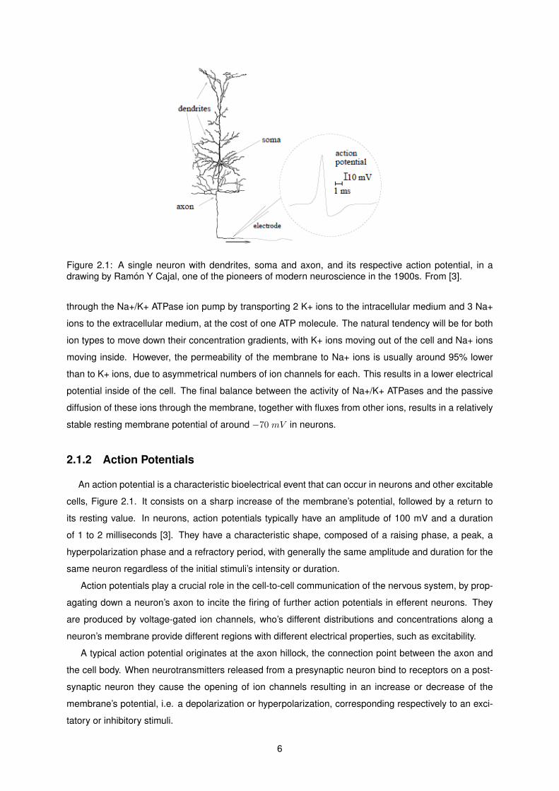
Figure 2.1: A single neuron with dendrites, soma and axon, and its respective action potential, in adrawing by Ramon Y Cajal, one of the pioneers of modern neuroscience in the 1900s. From [3].
through the Na+/K+ ATPase ion pump by transporting 2 K+ ions to the intracellular medium and 3 Na+
ions to the extracellular medium, at the cost of one ATP molecule. The natural tendency will be for both
ion types to move down their concentration gradients, with K+ ions moving out of the cell and Na+ ions
moving inside. However, the permeability of the membrane to Na+ ions is usually around 95% lower
than to K+ ions, due to asymmetrical numbers of ion channels for each. This results in a lower electrical
potential inside of the cell. The final balance between the activity of Na+/K+ ATPases and the passive
diffusion of these ions through the membrane, together with fluxes from other ions, results in a relatively
stable resting membrane potential of around −70 mV in neurons.
2.1.2 Action Potentials
An action potential is a characteristic bioelectrical event that can occur in neurons and other excitable
cells, Figure 2.1. It consists on a sharp increase of the membrane’s potential, followed by a return to
its resting value. In neurons, action potentials typically have an amplitude of 100 mV and a duration
of 1 to 2 milliseconds [3]. They have a characteristic shape, composed of a raising phase, a peak, a
hyperpolarization phase and a refractory period, with generally the same amplitude and duration for the
same neuron regardless of the initial stimuli’s intensity or duration.
Action potentials play a crucial role in the cell-to-cell communication of the nervous system, by prop-
agating down a neuron’s axon to incite the firing of further action potentials in efferent neurons. They
are produced by voltage-gated ion channels, who’s different distributions and concentrations along a
neuron’s membrane provide different regions with different electrical properties, such as excitability.
A typical action potential originates at the axon hillock, the connection point between the axon and
the cell body. When neurotransmitters released from a presynaptic neuron bind to receptors on a post-
synaptic neuron they cause the opening of ion channels resulting in an increase or decrease of the
membrane’s potential, i.e. a depolarization or hyperpolarization, corresponding respectively to an exci-
tatory or inhibitory stimuli.
6
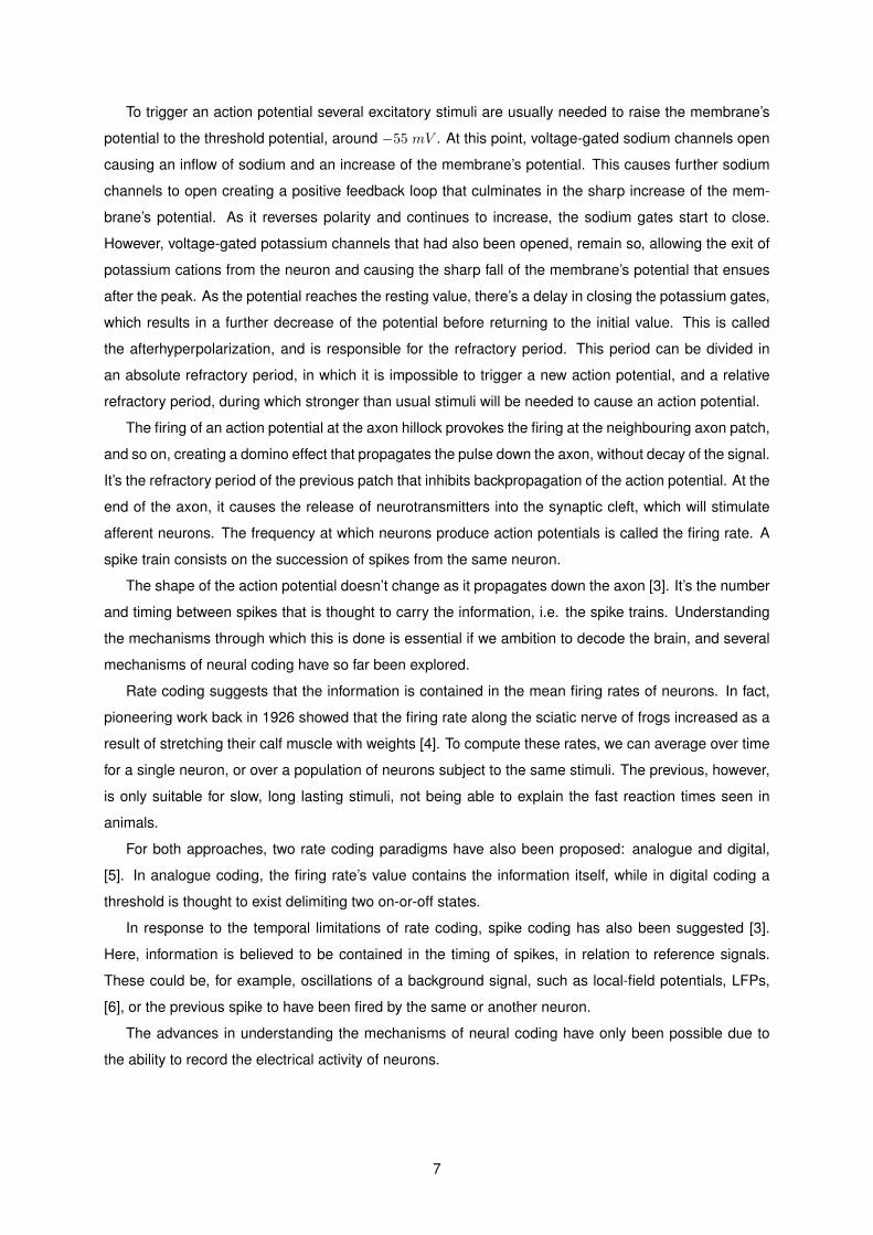
To trigger an action potential several excitatory stimuli are usually needed to raise the membrane’s
potential to the threshold potential, around −55 mV . At this point, voltage-gated sodium channels open
causing an inflow of sodium and an increase of the membrane’s potential. This causes further sodium
channels to open creating a positive feedback loop that culminates in the sharp increase of the mem-
brane’s potential. As it reverses polarity and continues to increase, the sodium gates start to close.
However, voltage-gated potassium channels that had also been opened, remain so, allowing the exit of
potassium cations from the neuron and causing the sharp fall of the membrane’s potential that ensues
after the peak. As the potential reaches the resting value, there’s a delay in closing the potassium gates,
which results in a further decrease of the potential before returning to the initial value. This is called
the afterhyperpolarization, and is responsible for the refractory period. This period can be divided in
an absolute refractory period, in which it is impossible to trigger a new action potential, and a relative
refractory period, during which stronger than usual stimuli will be needed to cause an action potential.
The firing of an action potential at the axon hillock provokes the firing at the neighbouring axon patch,
and so on, creating a domino effect that propagates the pulse down the axon, without decay of the signal.
It’s the refractory period of the previous patch that inhibits backpropagation of the action potential. At the
end of the axon, it causes the release of neurotransmitters into the synaptic cleft, which will stimulate
afferent neurons. The frequency at which neurons produce action potentials is called the firing rate. A
spike train consists on the succession of spikes from the same neuron.
The shape of the action potential doesn’t change as it propagates down the axon [3]. It’s the number
and timing between spikes that is thought to carry the information, i.e. the spike trains. Understanding
the mechanisms through which this is done is essential if we ambition to decode the brain, and several
mechanisms of neural coding have so far been explored.
Rate coding suggests that the information is contained in the mean firing rates of neurons. In fact,
pioneering work back in 1926 showed that the firing rate along the sciatic nerve of frogs increased as a
result of stretching their calf muscle with weights [4]. To compute these rates, we can average over time
for a single neuron, or over a population of neurons subject to the same stimuli. The previous, however,
is only suitable for slow, long lasting stimuli, not being able to explain the fast reaction times seen in
animals.
For both approaches, two rate coding paradigms have also been proposed: analogue and digital,
[5]. In analogue coding, the firing rate’s value contains the information itself, while in digital coding a
threshold is thought to exist delimiting two on-or-off states.
In response to the temporal limitations of rate coding, spike coding has also been suggested [3].
Here, information is believed to be contained in the timing of spikes, in relation to reference signals.
These could be, for example, oscillations of a background signal, such as local-field potentials, LFPs,
[6], or the previous spike to have been fired by the same or another neuron.
The advances in understanding the mechanisms of neural coding have only been possible due to
the ability to record the electrical activity of neurons.
7
2.2 Neural Interfaces
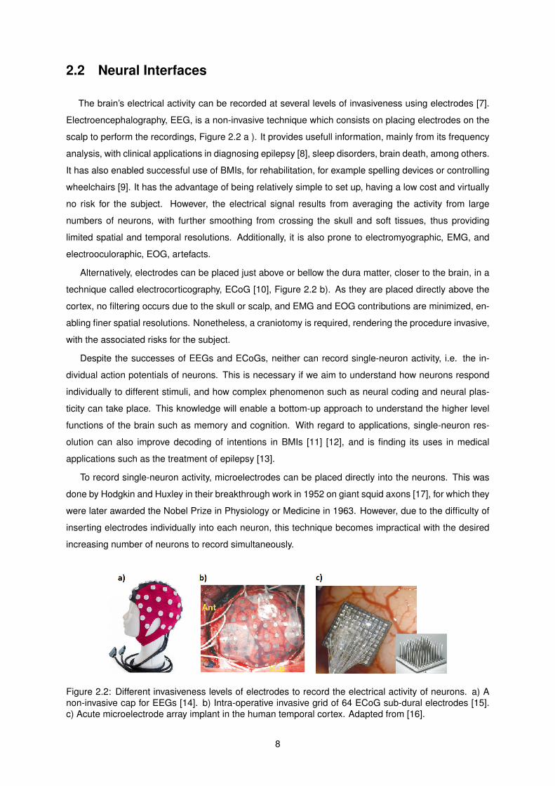
The brain’s electrical activity can be recorded at several levels of invasiveness using electrodes [7].
Electroencephalography, EEG, is a non-invasive technique which consists on placing electrodes on the
scalp to perform the recordings, Figure 2.2 a ). It provides usefull information, mainly from its frequency
analysis, with clinical applications in diagnosing epilepsy [8], sleep disorders, brain death, among others.
It has also enabled successful use of BMIs, for rehabilitation, for example spelling devices or controlling
wheelchairs [9]. It has the advantage of being relatively simple to set up, having a low cost and virtually
no risk for the subject. However, the electrical signal results from averaging the activity from large
numbers of neurons, with further smoothing from crossing the skull and soft tissues, thus providing
limited spatial and temporal resolutions. Additionally, it is also prone to electromyographic, EMG, and
electrooculoraphic, EOG, artefacts.
Alternatively, electrodes can be placed just above or bellow the dura matter, closer to the brain, in a
technique called electrocorticography, ECoG [10], Figure 2.2 b). As they are placed directly above the
cortex, no filtering occurs due to the skull or scalp, and EMG and EOG contributions are minimized, en-
abling finer spatial resolutions. Nonetheless, a craniotomy is required, rendering the procedure invasive,
with the associated risks for the subject.
Despite the successes of EEGs and ECoGs, neither can record single-neuron activity, i.e. the in-
dividual action potentials of neurons. This is necessary if we aim to understand how neurons respond
individually to different stimuli, and how complex phenomenon such as neural coding and neural plas-
ticity can take place. This knowledge will enable a bottom-up approach to understand the higher level
functions of the brain such as memory and cognition. With regard to applications, single-neuron res-
olution can also improve decoding of intentions in BMIs [11] [12], and is finding its uses in medical
applications such as the treatment of epilepsy [13].
To record single-neuron activity, microelectrodes can be placed directly into the neurons. This was
done by Hodgkin and Huxley in their breakthrough work in 1952 on giant squid axons [17], for which they
were later awarded the Nobel Prize in Physiology or Medicine in 1963. However, due to the difficulty of
inserting electrodes individually into each neuron, this technique becomes impractical with the desired
increasing number of neurons to record simultaneously.
Figure 2.2: Different invasiveness levels of electrodes to record the electrical activity of neurons. a) Anon-invasive cap for EEGs [14]. b) Intra-operative invasive grid of 64 ECoG sub-dural electrodes [15].c) Acute microelectrode array implant in the human temporal cortex. Adapted from [16].
8
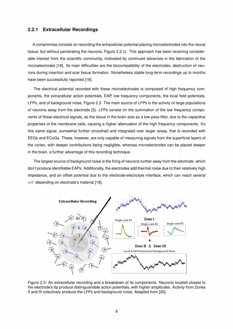
2.2.1 Extracellular Recordings
A compromise consists on recording the extracellular potential placing microelectrodes into the neural
tissue, but without penetrating the neurons, Figure 2.2 c). This approach has been receiving consider-
able interest from the scientific community, motivated by continued advances in the fabrication of the
microelectrodes [18]. Its main difficulties are the biocompatibility of the electrodes, destruction of neu-
rons during insertion and scar tissue formation. Nonetheless stable long-term recordings up to months
have been successfully reported [19].
The electrical potential recorded with these microelectrodes is composed of high frequency com-
ponents, the extracellular action potentials, EAP, low frequency components, the local field potentials,
LFPs, and of background noise, Figure 2.3. The main source of LFPs is the activity of large populations
of neurons away from the electrode [5]. LFPs consist on the summation of the low frequency compo-
nents of these electrical signals, as the tissue in the brain acts as a low-pass filter, due to the capacitive
properties of the membrane cells, causing a higher attenuation of the high frequency components. It’s
this same signal, somewhat further smoothed and integrated over larger areas, that is recorded with
EEGs and ECoGs. These, however, are only capable of measuring signals from the superficial layers of
the cortex, with deeper contributions being negligible, whereas microelectrodes can be placed deeper
in the brain, a further advantage of this recording technique.
The largest source of background noise is the firing of neurons further away from the electrode, which
don’t produce identifiable EAPs. Additionally, the electrodes add thermal noise due to their relatively high
impedance, and an offset potential due to the electrode-electrolyte interface, which can reach several
mV depending on electrode’s material [19].
Figure 2.3: An extracellular recording and a breakdown of its components. Neurons located closest tothe electrode’s tip produce distinguishable action potentials, with higher amplitudes. Activity from ZonesII and III colectively produce the LFPs and background noise. Adapted from [20].
9
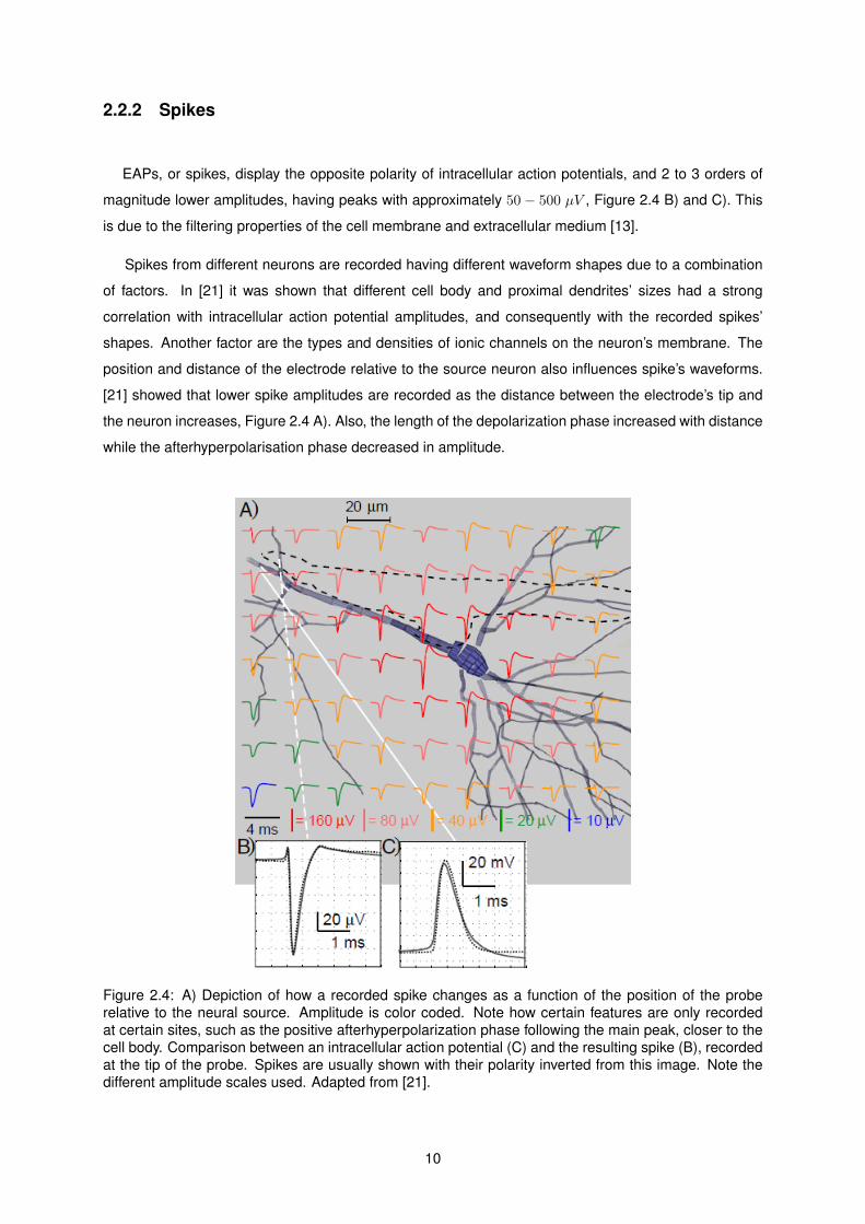
2.2.2 Spikes
EAPs, or spikes, display the opposite polarity of intracellular action potentials, and 2 to 3 orders of
magnitude lower amplitudes, having peaks with approximately 50 − 500 µV , Figure 2.4 B) and C). This
is due to the filtering properties of the cell membrane and extracellular medium [13].
Spikes from different neurons are recorded having different waveform shapes due to a combination
of factors. In [21] it was shown that different cell body and proximal dendrites’ sizes had a strong
correlation with intracellular action potential amplitudes, and consequently with the recorded spikes’
shapes. Another factor are the types and densities of ionic channels on the neuron’s membrane. The
position and distance of the electrode relative to the source neuron also influences spike’s waveforms.
[21] showed that lower spike amplitudes are recorded as the distance between the electrode’s tip and
the neuron increases, Figure 2.4 A). Also, the length of the depolarization phase increased with distance
while the afterhyperpolarisation phase decreased in amplitude.
Figure 2.4: A) Depiction of how a recorded spike changes as a function of the position of the proberelative to the neural source. Amplitude is color coded. Note how certain features are only recordedat certain sites, such as the positive afterhyperpolarization phase following the main peak, closer to thecell body. Comparison between an intracellular action potential (C) and the resulting spike (B), recordedat the tip of the probe. Spikes are usually shown with their polarity inverted from this image. Note thedifferent amplitude scales used. Adapted from [21].
10
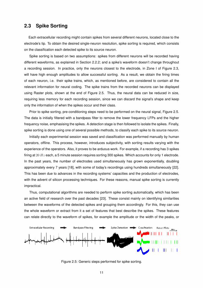
2.3 Spike Sorting
Each extracellular recording might contain spikes from several different neurons, located close to the
electrode’s tip. To obtain the desired single-neuron resolution, spike sorting is required, which consists
on the classification each detected spike to its source neuron.
Spike sorting is based on two assumptions: spikes from different neurons will be recorded having
different waveforms, as explained in Section 2.2.2; and a spike’s waveform doesn’t change throughout
a recording session. In practice, only the neurons closest to the electrode, in Zone I of Figure 2.3,
will have high enough amplitudes to allow successful sorting. As a result, we obtain the firing times
of each neuron, i.e. their spike trains, which, as mentioned before, are considered to contain all the
relevant information for neural coding. The spike trains from the recorded neurons can be displayed
using Raster plots, shown at the end of Figure 2.5. Thus, the neural data can be reduced in size,
requiring less memory for each recording session, since we can discard the signal’s shape and keep
only the information of when the spikes occur and their class.
Prior to spike sorting, pre-conditioning steps need to be performed on the neural signal, Figure 2.5.
The data is initially filtered with a bandpass filter to remove the lower frequency LFPs and the higher
frequency noise, emphasising the spikes. A detection stage is then followed to isolate the spikes. Finally,
spike sorting is done using one of several possible methods, to classify each spike to its source neuron.
Initially each experimental session was saved and classification was performed manually by human
operators, offline. This process, however, introduces subjectivity, with sorting results varying with the
experience of the operators. Also, it proves to be arduous work. For example, if a recording has 3 spikes
firing at 20Hz each, a 5 minute session requires sorting 300 spikes. Which accounts for only 1 electrode.
In the past years, the number of electrodes used simultaneously has grown exponentially, doubling
approximately every 7 years [18], with some of today’s recordings using hundreds simultaneously [22].
This has been due to advances in the recording systems’ capacities and the production of electrodes,
with the advent of silicon processing techniques. For these reasons, manual spike sorting is currently
impractical.
Thus, computational algorithms are needed to perform spike sorting automatically, which has been
an active field of research over the past decades [23]. These consist mainly on identifying similarities
between the waveforms of the detected spikes and grouping them accordingly. For this, they can use
the whole waveform or extract from it a set of features that best describe the spikes. These features
can relate directly to the waveform of spikes, for example the amplitude or the width of the peaks, or
Figure 2.5: Generic steps performed for spike sorting.
11
they can result from analytical methods, such as principal component analysis, PCA, or discrete wavelet
transform, DWT.
Feature extraction can additionally enable reducing the amount of data required to describe each
spike, and consequently lower the computational requirements of the classification stage. For example,
a spike composed of N samples could be represented by a set of M features, with M < N .
Spike sorting algorithms can be divided into two main types: offline and online, or real-time. Offline
methods consist on recording the whole session and then performing spike sorting on a computer. The
spikes are detected and projected onto the feature space, where clustering methods are used to group
them together. Spikes are classified according to the cluster where they end, with the assumption that
each cluster corresponds to a different source neuron. By being offline there are few time constraints,
allowing the use of computationally intensive methods. Additionally, they can use the whole recording
simultaneously. Thus, these methods are more likely to obtain better sorting results. In [24] a comparison
of spike sorting algorithms with publicly available source code showed how offline methods outperformed
an online method.
However, offline algorithms are not adequate for cases where real-time sorting results are required.
These are, for example, neural closed-loop experiments, where the procedure is adapted to real-time
feedback, and all BMIs, for the obvious reasons.
For these applications, online spike sorting is required, which is the focus of this thesis. The main
difference to offline spike sorting is that spikes need to be classified as they are detected, i.e. we can
not collect all the spikes prior to sorting. Additionally, real-time execution restricts the computational
complexity of the algorithms that can be used. For these reasons, the sorting algorithm is usually
divided into two stages: the training and the classification stage. During the training phase, somewhat
analogous to offline spike sorting, an initial segment of data is used for clustering, to find the underlying
model of the recording, i.e. the number of identifiable neurons in each channel and their corresponding
spike waveforms. With this information, a computationally lighter classifier is built, which is then used in
real-time during the classification stage, to sort each newly detected spike.
2.3.1 Challenges
Spike sorting is not a trivial task. Beyond the noise present in the recordings, which can corrupt
the waveforms of spikes, it faces many challenges. As the number of source neurons in each chan-
nel increases, differences between their waveforms become more subtle, rendering spike sorting more
difficult. In [25], three expert operators independently used a publicly available offline spike sorting soft-
ware, WaveClus [26], on different datasets with increasing numbers of source neurons. It revealed that
performances started to decline for more than 8 neurons per channel.
This may be one reason for the discrepancy between the number of neurons usually found in extra-
cellular recordings and their expected numbers, based on anatomical and biophysical considerations.
For example, at least 50 neurons would be expected per recording from the cat’s visual cortex, while
in practice they are approximately 10 fold fewer [27]. Further reasons for such discrepancy might be
12

neuron damage from probe insertion or the development of connective tissue insulating the probe after
insertion [28]. Additionally, it has been shown that the brain might be much less active than commonly
believed, having large numbers of sparsely firing neurons [27]. These might not produce enough spikes
during a recording session to create their own cluster, thus being misclassified.
Another challenge is overlapping spikes. These occur when neighbouring neurons fire closely in
time resulting in the superposition of their waveforms, which are difficult to disentangle. If neurons
consistently fire synchronously, the resulting combined waveform might even be attributed to a ‘false’
neuron [28].
The underlying premise of spike sorting, that the recorded spikes from a certain neuron do not
change over time, might also not hold under all circumstances. Some types of neurons fire in bursts -
sequences of closely spaced spikes, during which their amplitude decreases. This might cause them
to be erroneously sorted into different classes [28]. Analysis based on the firing times might be able to
correct theses cases, albeit not in real-time nor without an additional computational overhead. Electrode
drifting, i.e. movement of the electrode with respect to the neural tissue, might also cause the spike’s
shape to change, resulting in new clusters to appear and existing ones to split, merge or disappear [23].
This can occur, for example, in experiments with freely moving subjects, or from tissue retraction after
electrode insertion1. Additional waveform changes can also result from glial cell growth surrounding
the electrode tip, or connective tissue encapsulation. These phenomenon might require the sorting
algorithms to be adaptive, specially if targeting chronic implants or long experimental setups.
Adaptability can be partly achieved by successsively repeating the training phase, though it might
prove tricky to determine when to do so, or to relate the classes between consecutive trainings. With
offline spike sorting methods specifically, this problem can be tackled with non-parametric clustering
techniques, which can track these changes so long as they are gradual [28]. Parametric clustering
methods usually assume a model for the clusters, described by a set of parameters, for example, the
average and standard deviation of Gaussian distributions. However, as the waveforms of spikes change,
the resulting clusters might have unusual shapes, not fitting the typical models, and thus being better
suited for non-parametric clustering.
As mentioned earlier, we are also facing a constant increase in the number of channels to be
recorded simultaneously, currently reaching hundreds [22]. The increasing amounts of data produced
are putting pressure for the development of efficient spike sorting algorithms, specially for real-time ap-
plications. Additionally, shorter distances between electrodes, for example on tetrodes – probes with
4 closely positioned electrodes with distances usually of 25 − 50 µm, and high density multielectrode
arrays, are producing potentially redundant data. If the same spikes are detected on several channels
simultaneously, this poses a problem in interpreting the results from traditional spike sorting algorithms
[23]. However, it could also reveal itself useful for untangling overlapping spikes, if these are detected
separately on different channels. These issues have only recently started to be taken into account [28].
1reason for which acquisitions are usually only made 30 to 60 minutes after inserting the probes [28].
13
2.3.2 Validating Results
A key aspect in the development of spike sorting algorithms is the ability to validate their results
and compare performances between methods. The increasing variety of proposed methods calls for
common reference tools for this purpose [29]. These can be divided in two according to the type of
dataset used: with or without ground-truth knowledge, i.e. the information of which spike fired at what
time.
Without ground-truth knowledge, the case with most extracellular recordings, this is not a straight
forward problem. One approach consists on analysing the results for biological plausibility. Finding
the distribution of interspike intervals for each cluster, we can check if the refractory period is being
respected, an indication of successful sorting [23]. Another approach consists on using internal data of
the spike sorting method itself. For example, with clustering algorithms different metrics can be used to
evaluate the overall clustering performances, such as cluster separation or the final cost function value,
providing an indication of the sorting quality.
In [29], several statistical measures were developed to evaluate sorting performances with a ‘black-
box’ approach regarding the specific algorithm used. These measures focused mainly on the stability
of the algorithms. For example, comparing the results obtained from re-running them with the same
data, or using cross-validation - using some parts of the dataset to train classifiers to use on a common
segment of data and then comparing results. An additional validation method is auxiliary spike addition
[29], which consists on adding spikes with known classes to the dataset at specific times, and observing
to which clusters they are classified.
With ground-truth knowledge, validating and comparing different methods becomes a simpler prob-
lem. By matching the results with the truth we can create a confusion matrix, from which several evalu-
ation metrics can be computed, such as percentages of false and missed detections, and classification
accuracy and precision. Ground-truth can be obtained from recording sessions where both intra- and
extracellular potentials are measured simultaneously. However, these are not very frequent, and have a
limited scope from the reasons explained in Section 2.2.
Alternatively, models describing neural geometry, firing patterns and biological and instrumentation
noise can be developed and used to create artificial datasets. Spike templates from real recordings can
also be added. These artificial datasets provide for the largest flexibility, allowing to easily manipulate
various parameters such as the number of source neurons, the similarities between their waveforms and
the levels and nature of the background noise. The challenge resides on creating datasets capable of
realistically reproducing the expected extracellular recordings.
14
2.4 On-Chip Spike Sorting
Initially, neural recordings were performed with the electrodes inserted in the brain and wires relaying
the data outside to rack-based acquisition systems. With continued developments in miniaturized elec-
tronic fabrication and novel ASIC technologies, it became possible to start integrating signal conditioning
steps such as amplification and filtering with the electrodes. This allows to improve signal-to-noise ratios,
SNR, by reducing movement artefacts and external interferences on the low amplitude neural signals.
There are two main constrains in the design of these neural implants. Their overall size needs to be
kept to a minimum, to reduce trauma from implantation, ideally being possible to integrate the chip at
the base of the electrodes. The power dissipation of these implants is also limited by the possible heat-
induced damage to the biological tissues, with the literature stating a maximum temperature increase
allowed of 1oC [30]. As a reference, in [30], an implanted ASIC and 100-electrode array were predicted,
from finite-element analysis and in vitro and in vivo experiments, to induce a temperature increase due
to power dissipation of 0.029 oC/µW . Thus a maximum power dissipation of 34 mW would be allowed
for this ASIC and electrode-array combination.
The use of transcutaneous wires to power the device and transmit the data, however, causes prob-
lems. Not only do these wires restrict the movement of the subjects to the vicinity of the external
memory/processing devices, they cause a susceptibility for infections. With the current trend shifting
from shorter term implants, to performing recordings over longer periods, ultimately aiming at chronic
implants for rehabilitation BMIs, transcutaneous wires are not desirable. To bypass their use, a wireless
data transmitter can be included to allow a fully implantable neural recording device [31]. Additionally, a
battery needs to be included, with a wireless power link optional if chronic implants are intended.
Due to the relatively high frequency of spikes and the fine resolutions needed to capture the details
in their waveforms, the amounts of data produced by these implants can be quite high. A system with
128 channels, for example, can easily require rates of 23 Mbps.
These high bandwidth requirements, together with the need to respect strict power consumptions,
create a bottleneck in the design of such wireless neural implants, with the channel count lagging in com-
parison with microelectrode design advances. A review of wireless links for neural implants developed
up to 2009 can be found in [32].
A solution to this problem consists on performing data reduction on-chip prior to transmission [33]. By
performing detection, the isolated spikes can be transmitted individually, as opposed to transmitting the
whole signal [34]. Furthermore, feature extraction can allow lighter representations of spikes, reducing
transmission datarates.
However, on-chip spike sorting can provide for the most drastic data, and consequently, power, re-
duction, Figure 2.6, and has thus been an active field of research for the past two decades [19]. As
single-neuron spike trains are already the desired input for many applications, implementing sorting on-
chip in real-time allows reducing the datarate without loss of relevant information. Datarate reductions in
the order of 200×, compared to the transmission of the whole signal, can be achieved [33]. For example,
a 64-channel recording system transmitting at 11 Mbps could be reduced to 50 kbps, if only the outputs
15

Figure 2.6: Estimates of power consumptions per channel required to wirelessly transmit, from left toright, raw data, detected spikes and spike sorting results. AFE corresponds to the power required forthe analogue-front-end (explained further on), DSP for the digital signal processing and Radio for thewireless link. Adapted from [33].
from a sorting algorithm were transmitted.
For on-chip spike sorting several stages need to be implemented, Figure 2.7. Firstly, an analogue-
front-end, AFE, performs the signal conditioning tasks of amplification, filtering and digitization. Then, a
spike detection algorithm isolates the spikes from the neural signal. Finally, spike sorting per se can be
done.
It starts with the extraction of features. Dimensionality reduction methods can follow to select a
smaller subset, with the objective of reducing computational costs of subsequent processing stages,
while retaining discriminability. During the training phase, unsupervised learning techniques use the
features to cluster the spikes from an initial data segment, the training set. Based on the classification
results, a classifier able to distinguish the different classes is calibrated. It is then used during the
classification phase to classify each newly detected spike in real-time.
Due to the computational complexity of clustering, some on-chip spike sorting systems have opted to
perform training off-chip [35][36]. Spikes are first detected on-chip and streamed outside to a computer,
where clustering is performed and the parameters for the classifier are found. These are then transmitted
back to the system, which, switching operation modes, starts to perform online spike sorting, outputting
only the classification results.
2.4.1 Analogue-Front-End
The AFE provides the interface between the electrodes and the digital signal processing, DSP, stages
of the neural implant. It performs amplification, filtering and digitization, and has a direct influence in the
performance of the following spike detection and sorting algorithms. Firstly, a low-noise amplifier, LNA,
is used to raise the potential of the spikes from microvolts to millivolts, relaxing the noise requirements of
the following electronics. It typically provides amplification gains of 50−200 over a 3−10 kHz bandwidth
[19].
Filtering is necessary to remove all the undesired frequency components from the extracellular
recording: DC offset, baseline drift, LFPs and high frequency noise. Additionally, it also prevents aliasing
16
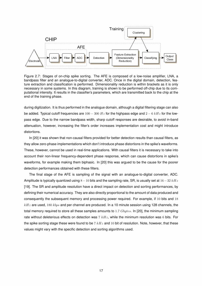
Figure 2.7: Stages of on-chip spike sorting. The AFE is composed of a low-noise amplifier, LNA, abandpass filter and an analogue-to-digital converter, ADC. Once in the digital domain, detection, fea-ture extraction and classification is performed. Dimensionality reduction is within brackets as it is onlynecessary in some systems. In this diagram, training is shown to be performed off-chip due to its com-putational intensity. It results in the classifier’s parameters, which are transmitted back to the chip at theend of the training phase.
during digitization. It is thus performed in the analogue domain, although a digital filtering stage can also
be added. Typical cutoff frequencies are 100− 300 Hz for the highpass edge and 2− 6 kHz for the low-
pass edge. Due to the narrow bandpass width, sharp cutoff responses are desirable, to avoid in-band
attenuation, however, increasing the filter’s order increases implementation cost and might introduce
distortions.
In [20] it was shown that non-causal filters provided for better detection results than causal filters, as
they allow zero-phase implementations which don’t introduce phase distortions in the spike’s waveforms.
These, however, cannot be used in real-time applications. With causal filters it is necessary to take into
account their non-linear frequency-dependent phase response, which can cause distortions in spike’s
waveforms, for example making them biphasic. In [20] this was argued to be the cause for the poorer
detection performances obtained with these filters.
The final stage of the AFE is sampling of the signal with an analogue-to-digital converter, ADC.
Amplitude is typically quantized using 8−10 bits and the sampling rate, SR, is usually set at 16−32 kHz
[19]. The SR and amplitude resolution have a direct impact on detection and sorting performances, by
defining their numerical accuracy. They are also directly proportional to the amount of data produced and
consequently the subsequent memory and processing power required. For example, if 10 bits and 18
kHz are used, 180 kbps and per channel are produced. In a 10 minute session using 128 channels, the
total memory required to store all these samples amounts to 1.7 Gbytes. In [20], the minimum sampling
rate without deleterious effects on detection was 7 kHz, while the minimum resolution was 6 bits. For
the spike sorting stage these were found to be 7 kHz and 10 bit of resolution. Note, however, that these
values might vary with the specific detection and sorting algorithms used.
17
2.4.2 Spike Detection
Once in the digital domain, signal detection algorithms isolate spikes from the recording. Beyond the
detected spikes these methods can originate both false positives - detections which do not correspond
to a spike, and false negatives - spikes that were not detected. The performance of detection has a
direct influence in the following spike sorting stage. However, if spike sorting is robust, we can allow
detection to be relaxed, having the false positives distinguished in the sorting stage by classifying them
as outliers.
Spike detection results in 2 or 3 ms long windows of data, each considered to contain an individual
spike, that are forwarded for spike sorting. The length of these windows should not be too small, to
contain the whole spike waveform, nor too big so as to avoid containing waveforms from more than
one spike. The window produced with each detection can start at the point of detection. However, this
will result in the loss of the initial part of the waveform, which can worsen spike sorting, for example
by missing the initial positive peak shown in some spikes in Figure 2.4. Alternatively, a rolling data
buffer can be used to save the previous X samples at any instant. Once detection occurs, these can
be retrieved and included in the data window. The downside is the need to constantly channel every
sample through this path, which results in higher costs2.
Most detection methods consist on applying a threshold to the neural signal, either directly or after an
operator has been applied to emphasise the spikes and attenuate the noise. A spike is considered to be
present if the threshold is crossed. If set too high, smaller spikes might be missed, but if too low, noise
activity might cause false positives. The threshold value can be set manually, although this becomes
impractical as the number of recording channels increases. Setting it automatically is thus preferable.
Additionally, this simplifies making detection adaptive to non-stationary noise levels throughout a record-
ing session, for example, by periodically recomputing the threshold’s value.
The most straightforward detection method consists on applying a threshold directly to the amplitude
of the signal. The threshold can be automatically set as a multiple of the standard deviation of the
background noise, which itself can be estimated by the standard deviation of the whole signal. With this
approach, however, the activity of neurons will have an influence on the threshold, with higher amplitude
and firing rate spikes shifting the threshold to higher values independent of noise levels. In [26] a different
estimate of the background noise level was proposed. Assuming the noise has a Gaussian distribution,
its standard deviation can be estimated from the whole signal as:
θn = median
{|x|
0.6745
}(2.1)
The denominator corresponds to the value of the cumulative distribution function of a standard normal
distribution evaluated at 0.75. By using the median, the contribution of spikes in the data is reduced.
It was shown in [26] that when firing rates increased, this method provided for a better estimate of the
standard deviation of the background noise than using the standard deviation of the whole signal. The
detection threshold can then be set as:
2in offline systems, as all the data is readily available, this isn’t a problem.
18
ThrD = X.θn (2.2)
With X determined empirically. The threshold can also be applied on the absolute value of the neural
signal, which has been reported to provide better detection performances than only using a positive
threshold [34].
While spikes are associated with changes in amplitude which are fast, the previous detection meth-
ods only account for the amplitude’s value itself, regardless of the derivative. For this reason, the
non-linear energy operator, NEO, also called Teager’s energy operator, has been proposed for spike
detection. It provides an estimate of a signal’s energy by applying the following operator:
ψ(x[n]) = x2[n]− x[n+ 1].x[n− 1] (2.3)
This results in the amplification of the signal where both the amplitude and frequency are high, how-
ever at an increased computational overhead. In [37] an automatic detection threshold was computed
as the average of the signal after applying the NEO, times a constant, C, that was empirically set to 8:
ThrD = C1
N
N∑n=1
ψ(x[n]) (2.4)
In [34] a cost function that took both detection performance and computational cost into account,
rendered absolute value detection more efficient than NEO, although different weights on the cost and
performance terms might result differently.
The discrete wavelet transform, DWT, has also been proposed for spike detection. By providing
energy information of the signal at different time-frequency windows, it is well suited for detection in
the presence of noise. However, its high implementation costs, with the computation of successive
convolutions, together with its worse detection performances compared with both absolute value and
NEO detectors in [37], excluded this method from our consideration.
Detection through match-filtering has also been proposed. It consists on sliding pre-determined spike
waveforms over the signal and detecting spikes when the mismatch is smaller than a certain value. It
requires, however, a priori knowledge of the spike waveforms, which is not ideal. Additionally, it carries
considerably high computational costs. In [34] it resulted in worse detection scores than both absolute
threshold and NEO detectors, precisely due to its high costs. When cost was not a constraint, it actually
performed better. Nevertheless, the need for a priori spike waveforms and its prohibitive computational
costs excluded this detection method from our consideration.
19

2.4.3 Spike Sorting Algorithms
Feature Extraction
Feature extraction results in the projection of spikes onto a feature space where spikes from different
neurons are better distinguishable. Additionally, it can lighten the computational cost of the following
stages, by representing spikes using fewer data.
The most straightforward approach is to use the samples of the spikes as features, i.e. without an
explicit feature extraction step. Hence, spike waveforms are compared directly with each other, a method
called template matching, TM [35].
Preceding TM with an alignment step has been suggested to improve sorting [38]. This can be easily
understood if we think of each feature as the value of a spike at a specific phase of its waveform. If the
waveform is shifted, the index of these features will not match. Spikes can be aligned to their maximum
by shifting so that the sample with highest value is at the ith position of the data window. Spikes can also
be aligned to the point where their derivative is maximum [39]. Alignment in real-time requires using,
during detection, the data buffer mentioned earlier. If no explicit alignment is done, it is equivalent to
aligning the spikes to detection point.
Since each spike can have many samples, a variation of TM consists on using only a smaller handful
of samples as opposed to using them all. These are called informative samples [40]. The principle
behind informative samples is that not all samples provide useful information to distinguish the spikes
from a recording, and if all are used, the useful information of some is diluted by the others. To find which
samples are informative in each channel, a dimensionality reduction method can be used, corresponding
to an additional step to perform during the training phase.
Other possbile features result directly from visible characteristics of the spikes’ waveforms. The
most intuitive are the extrema, i.e. the values of the maximum and the minimum, and the width of
the peaks [41]. In [42] it was argued that these lose their ability to sort spikes as the SNR of the
recording decreases. For this reason, they propose zero-crossing features, ZCF, as a combination of
their information. Two features are thus computed as:
ZCF1 =
Z−1∑n=0
x[n] ZCF2 =
K−1∑n=Z
x[n] (2.5)
K is the number of samples in each spike and Z is the index of the first zero-crossing after detection.
The integral transform has also been proposed to obtain a similar set of features to ZCF, [37]. It integrates
the samples for both the positive and negative peaks of the each spike, however, while with ZCF the
limit between the peaks is defined by the zero-crossing, with the integral transform the limits need to be
defined a priori :
IA =1
NA
nA+NA∑n=nA
x[n] IB =1
NB
nB+NB∑n=nB
x[n] (2.6)
A possible advantage is the ability to optimize these limits for the spike waveform combinations
present in each channel. However, this would most likely need to be performed offline.
20

Discrete derivatives, DD, can also be used as features, and are computed as the difference between
consecutive samples [37]:
DDδ = x[n]− x[n− δ] (2.7)
δ can take different integer values. The derivative operation can also be repeated to produce higher
order derivatives. Thus, many different features can be obtained, which introduces the need for a dimen-
sionality reduction method [39]. Alternatively, the extrema of each derivative can be used as the feature,
as was done in [43].
The discrete wavelet transform, DWT, as a feature extraction method, gained popularity due to the
offline spike sorting software made available in [26], WaveClus. The DWT is a multiresolution technique
which provides good temporal resolution for high frequencies and good frequency resolution for lower
frequencies. In real-time applications it can be computed through filter banks. However, the need to
perform successive convolutions results in considerably higher computational costs than the features
previously described. In [37] the DWT was studied for a possible hardware implementation. The Haar
wavelet family was used since it provided for the best results amongst the families tested, while also
being lighter to implement. However, it resulted in slightly lower sorting accuracies than DD while having
a computational cost more than 1 order of magnitude larger.
Principal component analysis, PCA, can also be used for feature extraction. It is most commonly
applied on the samples of spikes. Each spike can be represented by a point in a n-dimensional space
where each axis corresponds to a different sample index. PCA is a transformation applied on each of the
n-dimensional points which consists on projecting them onto n orthogonal vectors, the principal direc-
tions, resulting in n principal components, PCs. The principal directions are found as the eigenvectors
of the spikes. The first is aligned with the direction of largest variance in the dataset. The second is
aligned with the direction of largest variance orthogonal to the first principal direction, and so on. For
spike sorting, the first few PCs of each spike are used as features.
PCA is usually performed in offline systems, due to the high computational cost of computing the
principal directions. Nonetheless it can also be used in real-time applications where the training phase
is performed offline [37]. Storing the first few principal directions on-chip, they can be used during the
classification phase to compute the corresponding PCs of each detected spike. However, if each spike
has n samples and three PCs are to be used, these features require 3 × n multiplications plus 3 × n
additions.
Dimensionality Reduction
Dimensionality reduction, DR, is done whenever we wish to reduce the number of features to a
smaller, more informative subgroup. Beyond reducing the computational complexity of the following
stages, DR can also improve sorting accuracy [37]. If features without useful information are used, they
end up diluting the information of other relevant features during clustering. DR methods can be used
when studying which features are better suited for spike sorting. However, it has also been considered
21
for on-chip implementation, with the goal of developing truly unsupervised spike sorting platforms [37].
The most straightforward DR method is uniform subsampling. It was used in [39] to reduce the number
of features produced from DD. It consists simply on subsampling the feature space, without a selection
criteria, to produce a smaller subset.
In [37] a comparison between different DR methods for hardware implementation was done. As is
somewhat expected, uniform subsampling was not shown to produce good results. Another method
analysed was the Lilliefors test, which has previously been used in the offline spike sorting software
WaveClus. The underlying assumption is that multimodal features will result in better sorting perfor-
mances, with each lobe resulting from the activity of a different source neuron, as opposed to single
mode distributions where the features of all neurons are overlapped. The test consists on a modifica-
tion of the Kolmogorov-Smirnov test for normality. The empirical distribution function of each feature is
computed and compared with a normal distribution with the same mean and variance. The best feature
candidates are those with largest difference between both distributions.
Due to the computational intensity of the Lilliefors test, the maximum-difference test was also pro-
posed in [37]. It consists on identifying the best feature candidates as those with most variability, while
constrained by limited available memory. It was shown to perform similarly to the Lilliefors test in spite
of its lower computational cost.
Training Phase
The training phase is used to find the underlying model of the extracellular recording, i.e. the number
and characteristic waveform of each source neuron. This is most commonly achieved using clustering
methods. Their computational intensity has motivated a two-stage approach for on-chip spike sorting,
where clustering is performed offline on a computer, while only the classifier is implemented on-chip.
Possibly the most often used clustering method is k-means [33]. It randomly spreads k centroids in
the feature space then iteratively repeats the following steps: Assign each spike to the closest centroid,
based on the Euclidean distance; update the centroid as the average of the spikes assigned to it. With
TM, for example, each final centroid corresponds to the template spike waveform of each class. A
limitation of k-means is that the number of clusters, i.e. the number of source neurons, needs to be
provided a priori.
Other popular clustering algorithms used for spike sorting are expectation maximization, superpara-
magnetic clustering [26], Bayesian clustering and valley detection. For a detailed review of sorting
algorithms for biomedical applications, refer to [44].
The previous clustering methods are all performed offline, i.e. they requiring having all the data at
the beginning of clustering. In [45] a clustering algorithm, OSort, was developed for online spike sorting.
Additionally, it does not require prior knowledge of the number of source neurons expected, as with
k-means. It begins with the first spike producing the first cluster. Each new input spike is compared
with the existing cluster centroids using the Euclidean distance. It is then attributed to the closest cluster
if the distance is smaller than a threshold, computed from the variance of noise in the channel. This
cluster’s centroid is then updated using a weighted average. If the distance to every centroid is larger
22
than the threshold, the spike creates new cluster. At each iteration, the distance between the centroids
of each cluster is also computed, and if smaller than a threshold, clusters are merged together. With this
algorithm, many clusters are initially built, but with time they start to converge to a final, stable number.
Clustering can thus be performed in real-time, as spikes are detected.
Classification Phase
Once the spikes are clustered, different types of classifiers can be used for the classification phase.
These can be associated with the clustering method used in the first place. For example, with k-means,
the final centroids for each class can be stored on-chip. The distance between each new spike and these
centroids is computed and the spikes are classified to the closest centroid. Distance metrics that can be
used are the Euclidean distance and the L1-norm, among others [44]. Each has different computational
costs and properties. For example, in [33] it was argued that the L1-norm mas more robust to noise
compared with the Euclidean distance, in addition to being less computationally intensive to compute,
as no squaring operations are required. Other similarity measures can be used to compare each new
spike with the clusters obtained during the training phase [19].
Classification can also be achieved by separating the feature space into regions, each corresponding
to a different class. This can be implemented using decision trees, as was done in [46]. Alternatively,
in [36] each feature was compared individually with a pre-defined threshold to cast a binary vote, with
the majority defining the final classification of the spike. This approach facilitates using features having
different scales, such as spike amplitude and derivative. If used together to compute distances in the
feature space, the different scales would result in different features having different weights on the result.
2.4.4 State-of-the-Art
The main challenge of on-chip solutions is achieving the same performances as offline methods
while respecting the stringent power and area constrains. Neural recording platforms have been devel-
oped using either application specific integrated circuits, ASICs, or off-the-shelf components. The latter
have the advantage of being easier and faster to develop. Additionally, they facilitate adapting previous
systems to new spike sorting algorithms developed.
In [35] a field-programmable gate array, FPGA, was used to implement a two-stage spike sorting
algorithm. With it, spikes were detected by amplitude threshold crossing, and transmitted to a computer
via a USB 3.0 link, where WaveClus was used to cluster and determine the waveform templates for each
neuron. These were then sent back to the FPGA, where spike sorting by TM was performed in real-time.
During recordings, the power consumption was 32 mW for a total of 32 channels. This system, however,
is not implantable, intended to be incorporated on a headstage for animal experiments.
In [36] a similar two-stage approach was implemented using a microcontroller, MCU, where channel
specific, near-optimal features were found. These are a combination of informative samples and DD,
named waveform and derivative features. After offline clustering, during the training phase, an optimiza-
tion algorithm is used individually on each channel to find the subset from the features which provides
23

best separability between the spikes. Real-time classification is performed on the MCU by comparing
this smaller group of features with corresponding thresholds, also computed offline, to cast a vote, with
the majority determining the classification.
Artificial datasets with varying SNRs were used, to which white Gaussian noise was also added, to
simulate the contributions from the instrumentation. The performance-oriented dimensionality reduction
was shown to result in better sorting performances, while requiring lower costs, than other methods
such as PCA and DD, leaving the computational burden mainly to the offline, off-MCU stage. The MCU
managed 32 channels with a power consumption of 268 µW /channel. The authors mention, however,
that lower consumptions could be obtained with the development of an ASIC, estimated to consume only
34 µW /channel.
ASICs provide the best prospect for developing fully implantable, wireless, spike sorting systems.
In [41] a fully analogue IC was designed and built to perform spike detection and feature extraction. It
also included a LNA. Detection was achieved by thresholding both the positive and negative peaks of
spikes. The analogue features were obtained using capacitors and consisted on the maximum, minimum
and width of the main peak of each spike. Spike sorting was not included on-chip, however, using
real datasets from rats and monkeys the features were shown to achieve 90% of the sorting accuracy
obtained from PCA. The chip was implemented using a 0.35 µm CMOS process, occupying 0.24 mm2
and consuming 70 µW per channel.
In [39] a digital 64-channel spike detector and feature extractor was implemented. Fabricated in a 90
nm CMOS process, detection was done with NEO whose threshold was computed on-chip. Alignment
was done to the maximum derivative and the features were the DD. To reduce dimensionality, uniform
subsampling was performed, with a final data reduction of 11× being achieved compared with the trans-
mission of raw data. Using real data from a human epilepsy patient, these features resulted in sorting
results deemed acceptable by neuroscientists3. Using simulated datasets with SNRs ranging from −15
to 20 dB, the median probability of detection, probability of false positives and the sorting accuracy
where 87%, 5% and 77% respectively. The 64-channel chip occupied an area of 7.07 mm2, equivalent to
0.06 mm2 per channel, and consumed 130 µW using a 24 kHz SR and a resolution of 8 bits/sample.
As the number of channels increases, specialized circuit architectures can be used to achieve re-
source optimization on-chip. This was explored in [47] where a a mixture of parallel and serialized
processing enabled a 91% hardware cost (area × power) reduction compared to a fully parallel imple-
mentation. The system was designed for a 90 nm CMOS process, with a total of 128 channels. Detection
was performed with NEO and DD features were extracted for sorting. It occupied an area of 1.26 mm2,
and at a SR of 40 kHz the total power consumption was 1.87 mW . This value, however, resulted from
synthesis estimates, as the system was not manufactured and measured.
The SR is tightly related with the performance of sorting and simultaneously to the power consump-
tion of a system. To address this issue, [48] designed a cubic-spline interpolator to be integrated with a
spike sorting processor. As detection does not require detailed waveform information, lower SR can be
used at this stage. However, higher SRs improve alignment and sorting. Thus, by following detection3as mentioned earlier, it isn’t straightforward to measure sorting performances using real datasets, without ground-truth knowl-
edge.
24

with an interpolator, the authors argue that a better power/accuracy trade-off can be obtained. It was
shown that with it, a system operating at 12.5 kHz could outperform one operating at 25 kHz in both ac-
curacy and power. Employing a NEO spike detectior, DWT and PCA for feature extraction and k-means
for clustering, the system consumed 87 µW , equivalent to 0.68 µW /channel. Note however that offline
training was performed on a computer to determine the detection threshold, the principal directions and
so on. The area occupied by the chip, fabricated in a 90 nm CMOS process, was 8.89 mm2.
In [33] the first and so far, to the extent of our knowledge, only spike sorting system with on-chip
unsupervised clustering was developed. Detection was achieved with absolute value thresholding, and
clustering was performed using the samples of the spikes themselves, i.e. TM. The online clustering
algorithm OSort was adapted, since using it directly resulted in higher power consumptions that simply
transmitting the detected spikes. This was mainly due to the large amount of memory required to store
the transient clusters produced during the training phase. Thus, some modifications were made on the
algorithm.
It starts by determining the detection and clustering thresholds. Then, clustering is performed se-
quentially for each channel, allowing to share the larger memory required for the transient clusters. Their
number was found to converge after 30 spikes on average. Instead of using the Euclidean distance, the
L1-norm was chosen, as it was shown to be more robust to noise and less computationally intensive.
After sequential training, the classifying stage is initiated simultaneously on all channels. Each new
spike is classified to the closest cluster using the L1-norm. Adaptability to variations in a channel is
achieved by measuring the distance between each spike and cluster it’s classified to. If it is larger than
a threshold, the training phase can be repeated for this channel individually.
Implemented with a 65 nm CMOS process, the 16-channel chip occupies a total area of 1.23 mm2
and consumes 75 µW of power, resulting in a power density of 67 µW/mm2, which is bellow recom-
mended values to avoid tissue damage. Running on 600 simulated datasets with a SNR ranging 0− 15
dB, the probability of detection, false positives and classification accuracy were 95%, 1% and 75% re-
spectively. On human neural data obtained from an epilepsy patient, the clustering results were in
accordance with what was expected by neuroscientists. The clustering performance was comparable to
offline algorithms such as k-means and superparamagnetic clustering, in spite of the disadvantage of
not having all the data at the beginning of clustering. Compared with [39], higher power consumptions
were obtained. However, the data reduction achieved was 20× larger, which should result in overall
lower power consumptions if including the wireless link.
The works cited in this brief review are summarized in Table 2.1. Spike sorting results are not
included due to the variety of ways these are presented, and types of datasets used, with some systems
not even including on-chip classification.
25
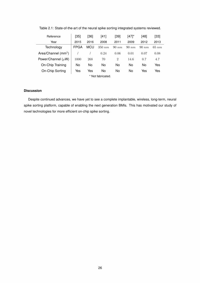
Table 2.1: State-of-the-art of the neural spike sorting integrated systems reviewed.
Reference [35] [36] [41] [39] [47]* [48] [33]
Year 2015 2016 2008 2011 2009 2012 2013
Technology FPGA MCU 350 nm 90 nm 90 nm 90 nm 65 nm
Area/Channel (mm2) / / 0.24 0.06 0.01 0.07 0.08
Power/Channel (µW) 1000 268 70 2 14.6 0.7 4.7
On-Chip Training No No No No No No Yes
On-Chip Sorting Yes Yes No No No Yes Yes
* Not fabricated.
Discussion
Despite continued advances, we have yet to see a complete implantable, wireless, long-term, neural
spike sorting platform, capable of enabling the next generation BMIs. This has motivated our study of
novel technologies for more efficient on-chip spike sorting.
26
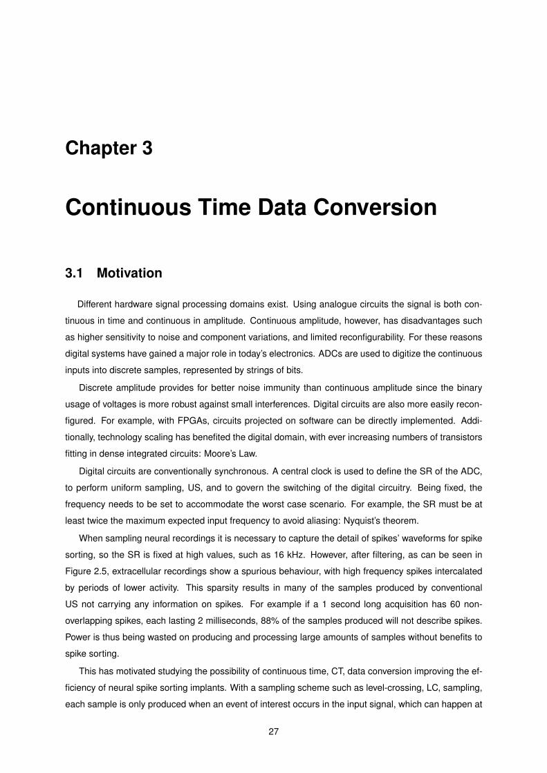
Chapter 3
Continuous Time Data Conversion
3.1 Motivation
Different hardware signal processing domains exist. Using analogue circuits the signal is both con-
tinuous in time and continuous in amplitude. Continuous amplitude, however, has disadvantages such
as higher sensitivity to noise and component variations, and limited reconfigurability. For these reasons
digital systems have gained a major role in today’s electronics. ADCs are used to digitize the continuous
inputs into discrete samples, represented by strings of bits.
Discrete amplitude provides for better noise immunity than continuous amplitude since the binary
usage of voltages is more robust against small interferences. Digital circuits are also more easily recon-
figured. For example, with FPGAs, circuits projected on software can be directly implemented. Addi-
tionally, technology scaling has benefited the digital domain, with ever increasing numbers of transistors
fitting in dense integrated circuits: Moore’s Law.
Digital circuits are conventionally synchronous. A central clock is used to define the SR of the ADC,
to perform uniform sampling, US, and to govern the switching of the digital circuitry. Being fixed, the
frequency needs to be set to accommodate the worst case scenario. For example, the SR must be at
least twice the maximum expected input frequency to avoid aliasing: Nyquist’s theorem.
When sampling neural recordings it is necessary to capture the detail of spikes’ waveforms for spike
sorting, so the SR is fixed at high values, such as 16 kHz. However, after filtering, as can be seen in
Figure 2.5, extracellular recordings show a spurious behaviour, with high frequency spikes intercalated
by periods of lower activity. This sparsity results in many of the samples produced by conventional
US not carrying any information on spikes. For example if a 1 second long acquisition has 60 non-
overlapping spikes, each lasting 2 milliseconds, 88% of the samples produced will not describe spikes.
Power is thus being wasted on producing and processing large amounts of samples without benefits to
spike sorting.
This has motivated studying the possibility of continuous time, CT, data conversion improving the ef-
ficiency of neural spike sorting implants. With a sampling scheme such as level-crossing, LC, sampling,
each sample is only produced when an event of interest occurs in the input signal, which can happen at
27
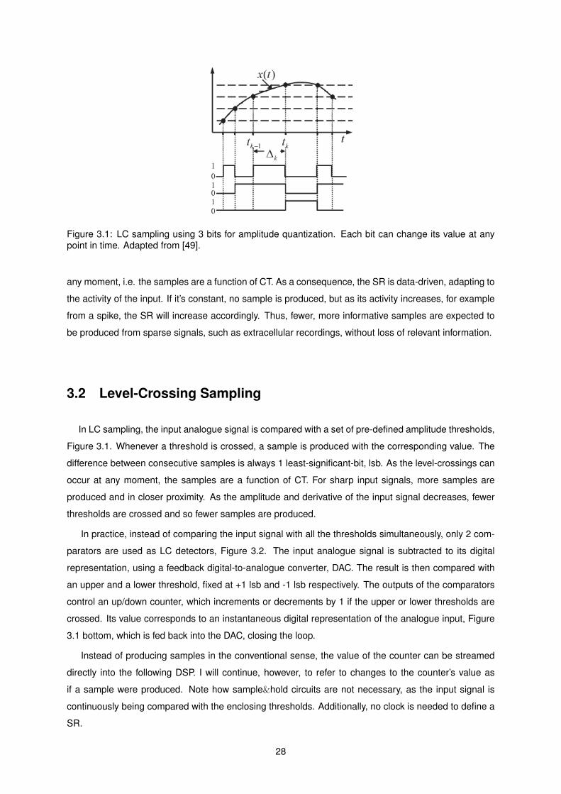
Figure 3.1: LC sampling using 3 bits for amplitude quantization. Each bit can change its value at anypoint in time. Adapted from [49].
any moment, i.e. the samples are a function of CT. As a consequence, the SR is data-driven, adapting to
the activity of the input. If it’s constant, no sample is produced, but as its activity increases, for example
from a spike, the SR will increase accordingly. Thus, fewer, more informative samples are expected to
be produced from sparse signals, such as extracellular recordings, without loss of relevant information.
3.2 Level-Crossing Sampling
In LC sampling, the input analogue signal is compared with a set of pre-defined amplitude thresholds,
Figure 3.1. Whenever a threshold is crossed, a sample is produced with the corresponding value. The
difference between consecutive samples is always 1 least-significant-bit, lsb. As the level-crossings can
occur at any moment, the samples are a function of CT. For sharp input signals, more samples are
produced and in closer proximity. As the amplitude and derivative of the input signal decreases, fewer
thresholds are crossed and so fewer samples are produced.
In practice, instead of comparing the input signal with all the thresholds simultaneously, only 2 com-
parators are used as LC detectors, Figure 3.2. The input analogue signal is subtracted to its digital
representation, using a feedback digital-to-analogue converter, DAC. The result is then compared with
an upper and a lower threshold, fixed at +1 lsb and -1 lsb respectively. The outputs of the comparators
control an up/down counter, which increments or decrements by 1 if the upper or lower thresholds are
crossed. Its value corresponds to an instantaneous digital representation of the analogue input, Figure
3.1 bottom, which is fed back into the DAC, closing the loop.
Instead of producing samples in the conventional sense, the value of the counter can be streamed
directly into the following DSP. I will continue, however, to refer to changes to the counter’s value as
if a sample were produced. Note how sample&hold circuits are not necessary, as the input signal is
continuously being compared with the enclosing thresholds. Additionally, no clock is needed to define a
SR.
28
Figure 3.2: Generic architecture of a LC ADC. The bold lines represent digital words. The value of theDAC is subtracted from the input analogue signal, which is then compared with the upper and lowerthresholds using two comparators whose outputs are fed into an up/down counter. If the differenceis within the thresholds, the output of both comparators is ‘0’, however, if it crosses either one, thecorresponding comparator raises to ‘1’. This will trigger the counter to update its value and consequentlythe value of the DAC, returning the difference back to within the thresholds. Adapted from [50].
3.2.1 Properties
The most relevant property of LC sampling for spike sorting is the SR being data-driven, i.e. adapting
to the activity of the input signal, as opposed to being fixed at the highest expected frequency. While
the designer of US ADCs defines both the SR and amplitude resolution, with CT LC ADCs only the
amplitude resolution, r, is defined:
r =VFS2N
(3.1)
VFS is the maximum input range and N the number of bits used for amplitude quantization. The
sampling rate of LC ADCs will depend solely on the relation between the amplitude resolution and
the input signal’s gradient and amplitude. This dynamic behaviour has the advantage of producing
few samples during the intervals between spikes, while continuing to samples these with the desired
amplitude resolution.
Overall less samples can thus be produced without losing information on spikes, reducing storage
and processing requirements, and leading to potential power savings. However, if the amplitude res-
olution is set too narrow, too many samples might be produced on the slopes of spikes. A balance is
required between the desired amplitude resolution and the number of samples produced.
For an sinusoidal input signal of amplitude A and frequency f , the number of samples generated per
second by a LC ADC is:
NS = 4A
rf (3.2)
If the input signal is Gaussian noise with bandwidth fm and power ϕ, the average number of samples
generated per second is [51]:
29
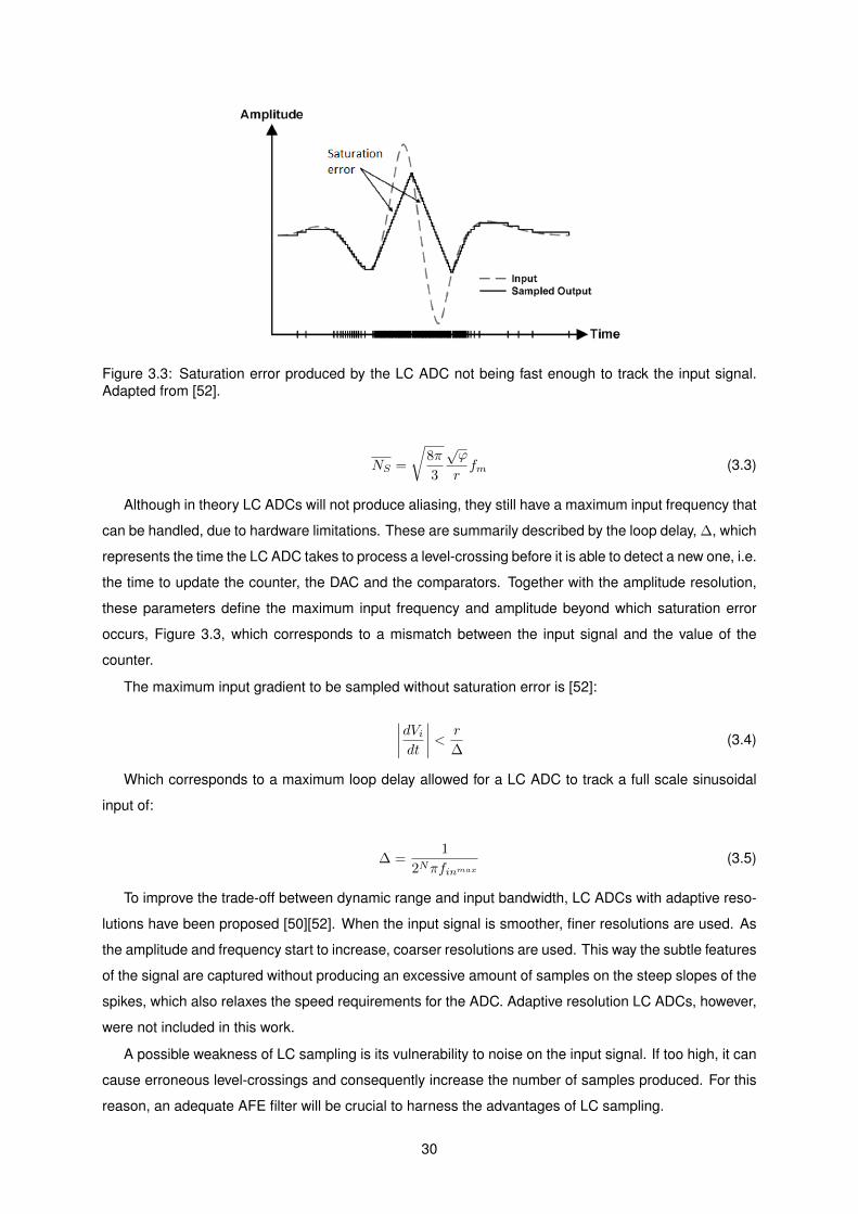
Figure 3.3: Saturation error produced by the LC ADC not being fast enough to track the input signal.Adapted from [52].
NS =
√8π
3
√ϕ
rfm (3.3)
Although in theory LC ADCs will not produce aliasing, they still have a maximum input frequency that
can be handled, due to hardware limitations. These are summarily described by the loop delay, ∆, which
represents the time the LC ADC takes to process a level-crossing before it is able to detect a new one, i.e.
the time to update the counter, the DAC and the comparators. Together with the amplitude resolution,
these parameters define the maximum input frequency and amplitude beyond which saturation error
occurs, Figure 3.3, which corresponds to a mismatch between the input signal and the value of the
counter.
The maximum input gradient to be sampled without saturation error is [52]:
∣∣∣∣dVidt∣∣∣∣ < r
∆(3.4)
Which corresponds to a maximum loop delay allowed for a LC ADC to track a full scale sinusoidal
input of:
∆ =1
2Nπfinmax
(3.5)
To improve the trade-off between dynamic range and input bandwidth, LC ADCs with adaptive reso-
lutions have been proposed [50][52]. When the input signal is smoother, finer resolutions are used. As
the amplitude and frequency start to increase, coarser resolutions are used. This way the subtle features
of the signal are captured without producing an excessive amount of samples on the steep slopes of the
spikes, which also relaxes the speed requirements for the ADC. Adaptive resolution LC ADCs, however,
were not included in this work.
A possible weakness of LC sampling is its vulnerability to noise on the input signal. If too high, it can
cause erroneous level-crossings and consequently increase the number of samples produced. For this
reason, an adequate AFE filter will be crucial to harness the advantages of LC sampling.
30

LC sampling can also result in lower quantization noise than US, [49]. In US, the analogue input at
each sample is rounded to the closest quantisation level, introducing some error . This is captured by
the theoretical SNR expression used to describe US ADCs: SNR = 6.02N + 1.76 dB.
N corresponds to the number of bits used for amplitude quantization. As it increases, the approxi-
mation error introduced in each sample is reduced and the SNR increases. With LC sampling, on the
other hand, each sample is only produced when the analogue input crosses a threshold, and so both
values coincide, meaning no rounding error is added1. Thus its spectrum will only have components at
the fundamental frequency of the input and its harmonics, while US results in many error spectral com-
ponents in between the harmonics. In [53] it was reported that the quantisation noise from LC sampling
a full-scale sinusoidal input of 1 kHz was −121 dB in a 20 kHz bandwidth, while US the same signal
resulted in −98 dB.
3.2.2 Asynchronous Delta-Modulation
A further advantage of using LC ADCs is that they enable a more economical representation of the
input signal. Proposed in 1966 [51], asynchronous-delta modulation consists on representing a signal
by a succession of binary pulses indicating whenever it has changed by a certain amount, and in which
direction the change occurred, Figure 3.4. These pulses can be directly obtained from the outputs
of the comparators of a LC ADC. If the upper or lower threshold is crossed, an incremental, INC, or
decremental, DEC, pulse is created respectively.
To facilitate the control of the following asynchronous DSP, explained in Chapter 4, the INC/DEC
pulses can be transformed, through some digital logic, into a request, REQ, and direction, DIR, pulses.
The REQ pulse indicates whenever any level-crossing occurs, and can be used as a control signal to
trigger the digital circuits, while the DIR indicates if it was an INC or DEC level-crossing. Thus the output
of LC ADCs is both the REQ and DIR pulses and the value of the counter, all of which are digital signals
but continuous in time.
Using asynchronous delta-modulation, the complexity of the following DSP stages can be signifi-
cantly reduced by allowing only 2-bit signal representations for certain data paths.
3.2.3 ADC State-of-Art: LC vs US
In this Section we compare the state-of-the-art of LC ADCs with their US counterparts. Different US
ADC architectures have been developed to achieve the best power consumptions at different SRs and
resolutions. To record electrophysiological signals, successive approximation register, SAR, ADCs are
the most appropriate [54].
SAR ADCs perform sampling through a binary search algorithm. First the analogue signal is captured
using a sample&hold circuit operating at the SR. The binary search is initiated by setting anN -bit register
to its midvalue - the most-significant-bit, MSB, at ’1’ while the remaining bits at ’0’. The length of the
1note however that the burden of time quantization is being transferred to the DSP. If we simply store the samples sequentiallyas is done in US, we loose this information.
31
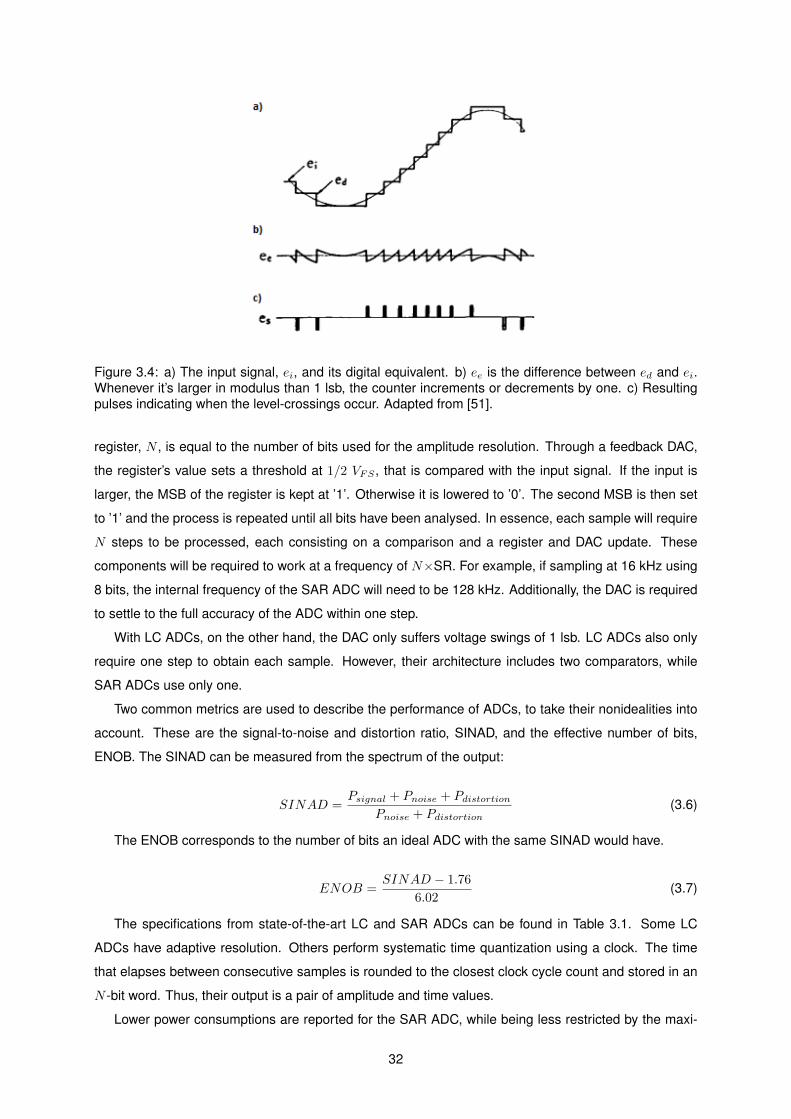
Figure 3.4: a) The input signal, ei, and its digital equivalent. b) ee is the difference between ed and ei.Whenever it’s larger in modulus than 1 lsb, the counter increments or decrements by one. c) Resultingpulses indicating when the level-crossings occur. Adapted from [51].
register, N , is equal to the number of bits used for the amplitude resolution. Through a feedback DAC,
the register’s value sets a threshold at 1/2 VFS , that is compared with the input signal. If the input is
larger, the MSB of the register is kept at ’1’. Otherwise it is lowered to ’0’. The second MSB is then set
to ’1’ and the process is repeated until all bits have been analysed. In essence, each sample will require
N steps to be processed, each consisting on a comparison and a register and DAC update. These
components will be required to work at a frequency of N×SR. For example, if sampling at 16 kHz using
8 bits, the internal frequency of the SAR ADC will need to be 128 kHz. Additionally, the DAC is required
to settle to the full accuracy of the ADC within one step.
With LC ADCs, on the other hand, the DAC only suffers voltage swings of 1 lsb. LC ADCs also only
require one step to obtain each sample. However, their architecture includes two comparators, while
SAR ADCs use only one.
Two common metrics are used to describe the performance of ADCs, to take their nonidealities into
account. These are the signal-to-noise and distortion ratio, SINAD, and the effective number of bits,
ENOB. The SINAD can be measured from the spectrum of the output:
SINAD =Psignal + Pnoise + Pdistortion
Pnoise + Pdistortion(3.6)
The ENOB corresponds to the number of bits an ideal ADC with the same SINAD would have.
ENOB =SINAD − 1.76
6.02(3.7)
The specifications from state-of-the-art LC and SAR ADCs can be found in Table 3.1. Some LC
ADCs have adaptive resolution. Others perform systematic time quantization using a clock. The time
that elapses between consecutive samples is rounded to the closest clock cycle count and stored in an
N -bit word. Thus, their output is a pair of amplitude and time values.
Lower power consumptions are reported for the SAR ADC, while being less restricted by the maxi-
32
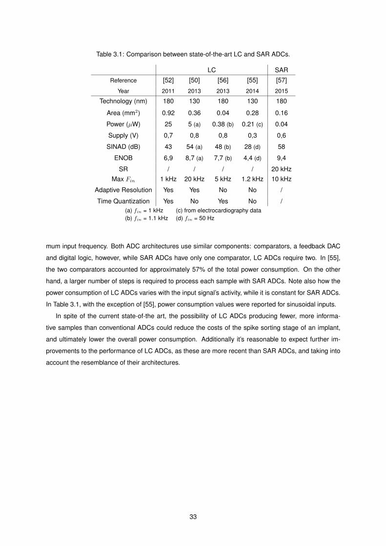
Table 3.1: Comparison between state-of-the-art LC and SAR ADCs.
LC SAR
Reference [52] [50] [56] [55] [57]
Year 2011 2013 2013 2014 2015
Technology (nm) 180 130 180 130 180
Area (mm2) 0.92 0.36 0.04 0.28 0.16
Power (µW) 25 5 (a) 0.38 (b) 0.21 (c) 0.04
Supply (V) 0,7 0,8 0,8 0,3 0,6
SINAD (dB) 43 54 (a) 48 (b) 28 (d) 58
ENOB 6,9 8,7 (a) 7,7 (b) 4,4 (d) 9,4
SR / / / / 20 kHzMax Fin 1 kHz 20 kHz 5 kHz 1.2 kHz 10 kHz
Adaptive Resolution Yes Yes No No /
Time Quantization Yes No Yes No /(a) fin = 1 kHz (c) from electrocardiography data(b) fin = 1.1 kHz (d) fin = 50 Hz
mum input frequency. Both ADC architectures use similar components: comparators, a feedback DAC
and digital logic, however, while SAR ADCs have only one comparator, LC ADCs require two. In [55],
the two comparators accounted for approximately 57% of the total power consumption. On the other
hand, a larger number of steps is required to process each sample with SAR ADCs. Note also how the
power consumption of LC ADCs varies with the input signal’s activity, while it is constant for SAR ADCs.
In Table 3.1, with the exception of [55], power consumption values were reported for sinusoidal inputs.
In spite of the current state-of-the art, the possibility of LC ADCs producing fewer, more informa-
tive samples than conventional ADCs could reduce the costs of the spike sorting stage of an implant,
and ultimately lower the overall power consumption. Additionally it’s reasonable to expect further im-
provements to the performance of LC ADCs, as these are more recent than SAR ADCs, and taking into
account the resemblance of their architectures.
33
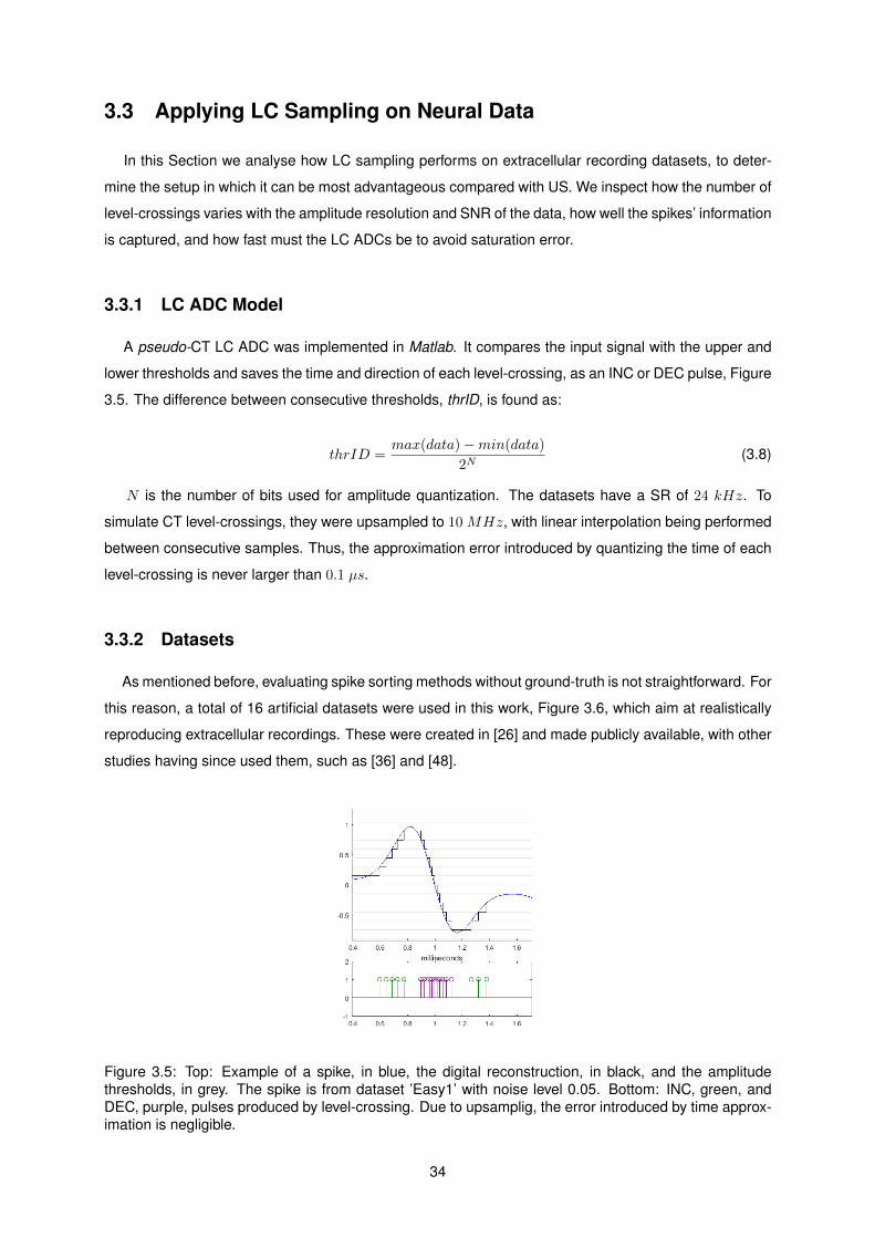
3.3 Applying LC Sampling on Neural Data
In this Section we analyse how LC sampling performs on extracellular recording datasets, to deter-
mine the setup in which it can be most advantageous compared with US. We inspect how the number of
level-crossings varies with the amplitude resolution and SNR of the data, how well the spikes’ information
is captured, and how fast must the LC ADCs be to avoid saturation error.
3.3.1 LC ADC Model
A pseudo-CT LC ADC was implemented in Matlab. It compares the input signal with the upper and
lower thresholds and saves the time and direction of each level-crossing, as an INC or DEC pulse, Figure
3.5. The difference between consecutive thresholds, thrID, is found as:
thrID =max(data)−min(data)
2N(3.8)
N is the number of bits used for amplitude quantization. The datasets have a SR of 24 kHz. To
simulate CT level-crossings, they were upsampled to 10 MHz, with linear interpolation being performed
between consecutive samples. Thus, the approximation error introduced by quantizing the time of each
level-crossing is never larger than 0.1 µs.
3.3.2 Datasets
As mentioned before, evaluating spike sorting methods without ground-truth is not straightforward. For
this reason, a total of 16 artificial datasets were used in this work, Figure 3.6, which aim at realistically
reproducing extracellular recordings. These were created in [26] and made publicly available, with other
studies having since used them, such as [36] and [48].
Figure 3.5: Top: Example of a spike, in blue, the digital reconstruction, in black, and the amplitudethresholds, in grey. The spike is from dataset ’Easy1’ with noise level 0.05. Bottom: INC, green, andDEC, purple, pulses produced by level-crossing. Due to upsamplig, the error introduced by time approx-imation is negligible.
34
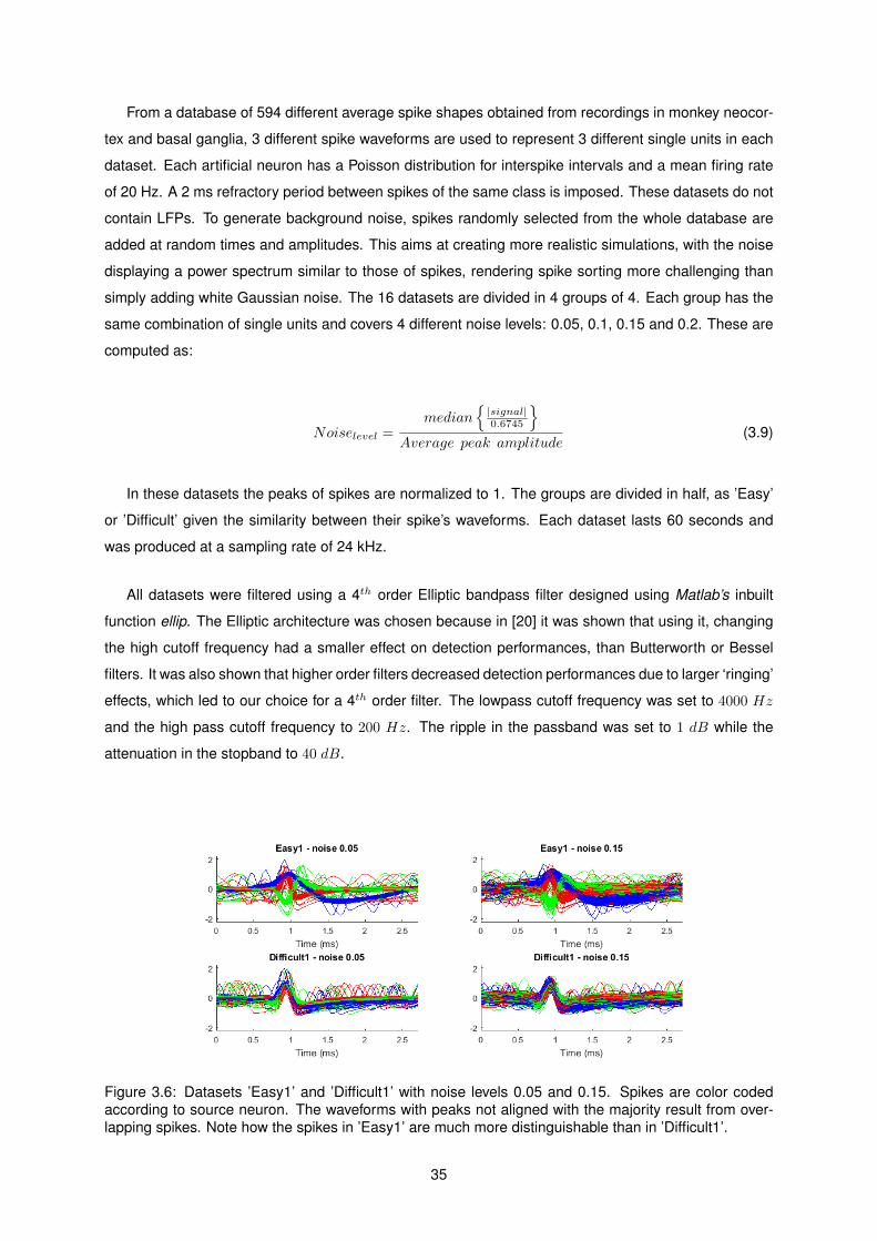
From a database of 594 different average spike shapes obtained from recordings in monkey neocor-
tex and basal ganglia, 3 different spike waveforms are used to represent 3 different single units in each
dataset. Each artificial neuron has a Poisson distribution for interspike intervals and a mean firing rate
of 20 Hz. A 2 ms refractory period between spikes of the same class is imposed. These datasets do not
contain LFPs. To generate background noise, spikes randomly selected from the whole database are
added at random times and amplitudes. This aims at creating more realistic simulations, with the noise
displaying a power spectrum similar to those of spikes, rendering spike sorting more challenging than
simply adding white Gaussian noise. The 16 datasets are divided in 4 groups of 4. Each group has the
same combination of single units and covers 4 different noise levels: 0.05, 0.1, 0.15 and 0.2. These are
computed as:
Noiselevel =median
{|signal|0.6745
}Average peak amplitude
(3.9)
In these datasets the peaks of spikes are normalized to 1. The groups are divided in half, as ’Easy’
or ’Difficult’ given the similarity between their spike’s waveforms. Each dataset lasts 60 seconds and
was produced at a sampling rate of 24 kHz.
All datasets were filtered using a 4th order Elliptic bandpass filter designed using Matlab’s inbuilt
function ellip. The Elliptic architecture was chosen because in [20] it was shown that using it, changing
the high cutoff frequency had a smaller effect on detection performances, than Butterworth or Bessel
filters. It was also shown that higher order filters decreased detection performances due to larger ‘ringing’
effects, which led to our choice for a 4th order filter. The lowpass cutoff frequency was set to 4000 Hz
and the high pass cutoff frequency to 200 Hz. The ripple in the passband was set to 1 dB while the
attenuation in the stopband to 40 dB.
Figure 3.6: Datasets ’Easy1’ and ’Difficult1’ with noise levels 0.05 and 0.15. Spikes are color codedaccording to source neuron. The waveforms with peaks not aligned with the majority result from over-lapping spikes. Note how the spikes in ’Easy1’ are much more distinguishable than in ’Difficult1’.
35
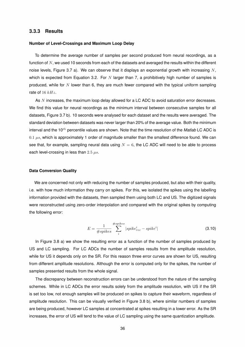
3.3.3 Results
Number of Level-Crossings and Maximum Loop Delay
To determine the average number of samples per second produced from neural recordings, as a
function ofN , we used 10 seconds from each of the datasets and averaged the results within the different
noise levels, Figure 3.7 a). We can observe that it displays an exponential growth with increasing N ,
which is expected from Equation 3.2. For N larger than 7, a prohibitively high number of samples is
produced, while for N lower than 6, they are much fewer compared with the typical uniform sampling
rate of 16 kHz.
As N increases, the maximum loop delay allowed for a LC ADC to avoid saturation error decreases.
We find this value for neural recordings as the minimum interval between consecutive samples for all
datasets, Figure 3.7 b). 10 seconds were analysed for each dataset and the results were averaged. The
standard deviation between datasets was never larger than 20% of the average value. Both the minimum
interval and the 10th percentile values are shown. Note that the time resolution of the Matlab LC ADC is
0.1 µs, which is approximately 1 order of magnitude smaller than the smallest difference found. We can
see that, for example, sampling neural data using N = 6, the LC ADC will need to be able to process
each level-crossing in less than 2.5 µs.
Data Conversion Quality
We are concerned not only with reducing the number of samples produced, but also with their quality,
i.e. with how much information they carry on spikes. For this, we isolated the spikes using the labelling
information provided with the datasets, then sampled them using both LC and US. The digitized signals
were reconstructed using zero-order interpolation and compared with the original spikes by computing
the following error:
E =1
#spikes
#spikes∑i
|spikeirec − spikei| (3.10)
In Figure 3.8 a) we show the resulting error as a function of the number of samples produced by
US and LC sampling. For LC ADCs the number of samples results from the amplitude resolution,
while for US it depends only on the SR. For this reason three error curves are shown for US, resulting
from different amplitude resolutions. Although the error is computed only for the spikes, the number of
samples presented results from the whole signal.
The discrepancy between reconstruction errors can be understood from the nature of the sampling
schemes. While in LC ADCs the error results solely from the amplitude resolution, with US if the SR
is set too low, not enough samples will be produced on spikes to capture their waveform, regardless of
amplitude resolution. This can be visually verified in Figure 3.8 b), where similar numbers of samples
are being produced, however LC samples at concentrated at spikes resulting in a lower error. As the SR
increases, the error of US will tend to the value of LC sampling using the same quantization amplitude.
36
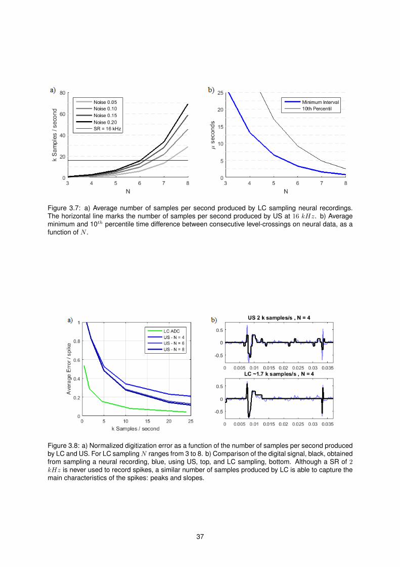
Figure 3.7: a) Average number of samples per second produced by LC sampling neural recordings.The horizontal line marks the number of samples per second produced by US at 16 kHz. b) Averageminimum and 10th percentile time difference between consecutive level-crossings on neural data, as afunction of N .
Figure 3.8: a) Normalized digitization error as a function of the number of samples per second producedby LC and US. For LC samplingN ranges from 3 to 8. b) Comparison of the digital signal, black, obtainedfrom sampling a neural recording, blue, using US, top, and LC sampling, bottom. Although a SR of 2kHz is never used to record spikes, a similar number of samples produced by LC is able to capture themain characteristics of the spikes: peaks and slopes.
37

3.3.4 Discussion
With the previous analysis we have observed how the numbers of samples produced by LC sampling
change with the amplitude quantization used, having identified 7 bits as the limit bellow which fewer
samples are produced from spurious neural data, compared to US systems.
We have also confirmed that at similar numbers of average samples per second, LC is better at
describing spikes than US due to its event-driven nature. Additionally, we inform LC ADC designers of
the timing requirements these need to satisfy for their application to extracellular recordings.
The use of CT LC sampling, however, raises challenges, namely how its outputs - the REQ and DIR
pulses and the counter’s value, can be used, with their timing information, for spike sorting. This is the
focus of the following Chapter.
38
Chapter 4
Asynchronous Spike Sorting
The CT nature of LC ADCs motivates the use of asynchronous digital circuitry for spike sorting, where
the data is processed as it arrives, in a self-timed manner.
As the circuit speed adapts, rather than being fixed at the speed mandated by the worst case, tran-
sistors will only switch when the input changes. This results in adaptive dynamic power consumption
that can lead to savings when processing spurious data, as extracellular recordings. A central clock to
set the SR and govern the DSP is also not required, enabling further savings by removing clock drivers,
avoiding the difficulties of distributing time-sensitive, high fan-out clock signals. This can also improve
modularity, for example for networks of low-power neural implants.
Electromagnetic interference, EMI, is also less severe than in synchronous systems. These produce
considerable EMI at the frequency band of the clock and its harmonics, while EMI patterns in asyn-
chronous circuits are much more evenly distributed across the spectrum. Finally, less stress on the
power distribution network is also achieved, as the power drawn tends to be more uniform, as opposed
to being bursty at the clock pulses.
This approach, however, has its challenges, such as the additional difficulty in circuit designing,
to manage the control pulses and avoid race conditions along the processing pipeline. Additionally,
unlike conventional asynchronous systems, the timing between the outputs of the CT LC ADC contains
information, which must be preserved during the signal processing stages.
Truly CT DSPs have been reported in the literature, using tapped digital delay lines to implement CT
digital FIR filters [58][59]. With these, the timing information is preserved as the signal flows down the
delay line, which acts as a sort of memory. However, due to the cost of implementing delay lines, we
have opted for explicit time quantization, at the feature extraction stage, effectively switching from the CT
domain to asynchronous, Figure 4.1. Time can be quantized through an oscillator and a counter. This
is the assumption made for our system, although the underlying technology is not explored in this work.
It is important, however, to be able to tune the oscillator’s frequency as it defines the time resolution.
39
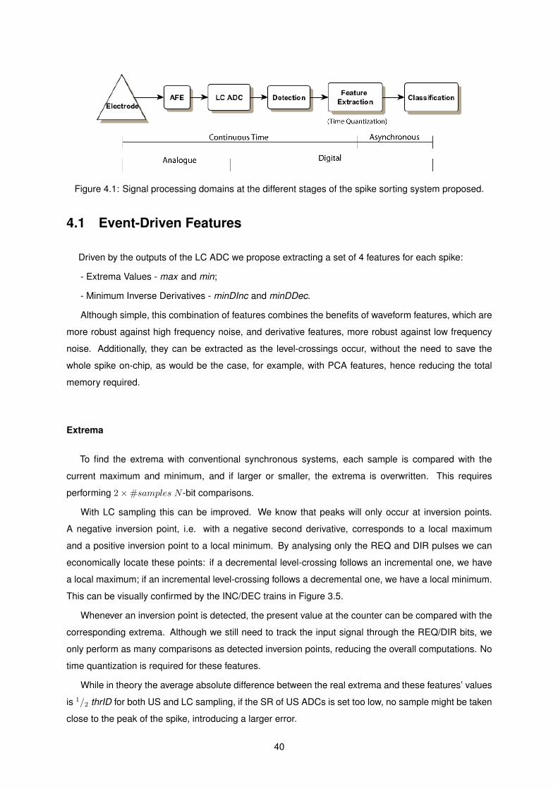
Figure 4.1: Signal processing domains at the different stages of the spike sorting system proposed.
4.1 Event-Driven Features
Driven by the outputs of the LC ADC we propose extracting a set of 4 features for each spike:
- Extrema Values - max and min;
- Minimum Inverse Derivatives - minDInc and minDDec.
Although simple, this combination of features combines the benefits of waveform features, which are
more robust against high frequency noise, and derivative features, more robust against low frequency
noise. Additionally, they can be extracted as the level-crossings occur, without the need to save the
whole spike on-chip, as would be the case, for example, with PCA features, hence reducing the total
memory required.
Extrema
To find the extrema with conventional synchronous systems, each sample is compared with the
current maximum and minimum, and if larger or smaller, the extrema is overwritten. This requires
performing 2×#samples N -bit comparisons.
With LC sampling this can be improved. We know that peaks will only occur at inversion points.
A negative inversion point, i.e. with a negative second derivative, corresponds to a local maximum
and a positive inversion point to a local minimum. By analysing only the REQ and DIR pulses we can
economically locate these points: if a decremental level-crossing follows an incremental one, we have
a local maximum; if an incremental level-crossing follows a decremental one, we have a local minimum.
This can be visually confirmed by the INC/DEC trains in Figure 3.5.
Whenever an inversion point is detected, the present value at the counter can be compared with the
corresponding extrema. Although we still need to track the input signal through the REQ/DIR bits, we
only perform as many comparisons as detected inversion points, reducing the overall computations. No
time quantization is required for these features.
While in theory the average absolute difference between the real extrema and these features’ values
is 1/2 thrID for both US and LC sampling, if the SR of US ADCs is set too low, no sample might be taken
close to the peak of the spike, introducing a larger error.
40
Minimum Inverse Derivatives
Commonly used features for spike sorting are the maximum of spikes’ derivatives. Due to the nature
of LC sampling, we propose extracting the minimum inverse derivatives instead. In synchronous digital
systems the derivative is found as:
∆xi∆t
=xi − xi−1ti − ti−1
= xi − xi−1 (4.1)
Since the time between consecutive samples is constant, it can be defined as 1 unit of time to
simplify the expression. In LC sampling, on the other hand, this interval is a function of CT, however, the
difference between consecutive samples is always 1 lsb. Thus, an inverse derivative can be computed
as:
∆ti∆x
=ti − ti−1xi − xi−1
= ti − ti−1 (4.2)
Each inverse derivative is obtained by measuring the time that elapses between consecutive level-
crossings. If the signal has a sharp increase, i.e. has a large derivative, this time will be short, resulting
in a small inverse derivative. A distinction can be made between the inverse derivative of consecutive
INC pulses and consecutive DEC pulses. The minima of these are the features: minDInc and minDDec.
This is the only stage of our system where time needs to be quantized. As we are only interested
on the minima of the inverse derivatives, time quantization can be performed only over a short interval,
outside of which we can assume the pulses in question do not produce a minimum.
While conventional derivatives require performing N -bit subtractions between consecutive samples,
the inverse derivatives only require manipulating the REQ and DIR pulses. However, time quantization
could prove costly.
4.2 Methodology
To analyse how spike sorting performs with the proposed event-driven features, EDF, we used 20
seconds of each dataset and the Matlab LC ADC model described in the previous Section.
Amplitude threshold crossing is used for detection, as methods such as NEO would require system-
atically saving the timing information of every level-crossing, increasing overall costs. With amplitude
thresholding, only the instantaneous value of the input is required. For the same reason, no pre-detection
buffer is used, so spikes are aligned to detection point. As the first dominant peak of all spikes in our
datasets is positive, only a positive detection threshold is used.
From Equations 2.1 and 2.2 the detection threshold for the noisiest datasets would be too high. For
this reason, it was fixed equally for all datasets at ThrD = 0.25, which corresponds to the value obtained
from the same equations applied to the least noisy datasets and fixing X = 5. The threshold value was
then rounded to the closest amplitude quantization level.
Using the labelling information provided with the datasets, perfect detection is done, rejecting false
41
positives and overlapping spikes, so as to better interpret the sorting results.
With each detection a 1 ms window is initiated, during which the features are extracted and used to
classify the spike. Perfect training is done by using the ground-truth knowledge to compute the centroids
of each class as the median of the spikes belonging to that class. The median was used as it was found
to result in better sorting performances than using the average.
The spikes were then classified to the closest centroid using the l1-norm:
Classj = mini||Featuresj − Centroidi||1 , i = 1, 2, 3 ; j = 1, ...,#spikes (4.3)
To evaluate performances we compute the accuracy of sorting as:
Accuracyi =TPi + TNiTotal
(4.4)
With TPi the number of spikes correctly classified to class i, TNi the number of spikes neither
belonging nor classified to class i and Total corresponding to the total number of spikes. The accuracy
results were averaged among the three spike classes.
To compare results with a typical US, synchronous spike sorting method, we sort the same spikes
using template matching, a method often seen in the literature as a reference. The same methodology is
repeated, i.e. perfect detection by amplitude threshold crossing, alignment to detection point and perfect
training.
We are interested not only on sorting performance, but also on the corresponding computational
cost. It’s measured by the number of operations, considering 1 operation as a 1-bit addition, subtraction
or comparison, or a modulus operation.
To extract the max and min features we require one 1-bit comparison per event (level-crossing) to
find the inversion points, plus one N -bit comparison per inversion point to determine the extrema, with
N being the number of bits used to quantize amplitude. The average number of events and inversion
points per spike will also depend on N :
Costmax+min = #events+ #inv.points×N operations (4.5)
For the minDInc and minDDec we need time quantization. This is done uniformly in discrete ∆t-wide
intervals, with the resulting values stored in M -bit words. For a fixed ∆t, M will define the range of
time quantization. ∆t mustn’t be larger than the minimum minDInc/Dec, represented by ∆tmax, which
depends on N , as seen in Equation 3.5. However, it can be smaller, improving time resolution, but,
for a fixed M , reducing the range. For each pair of events, an M -bit comparison is needed to find the
extrema:
CostminDInc+Dec = (#events− 1)×M operations + Time Quantization (4.6)
TM does not require computations for feature extraction, as these are the samples themselves.
However, a larger number of features are produced, increasing the memory of the system plus the
42
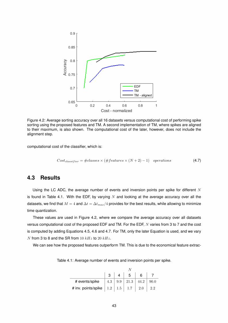
Figure 4.2: Average sorting accuracy over all 16 datasets versus computational cost of performing spikesorting using the proposed features and TM. A second implementation of TM, where spikes are alignedto their maximum, is also shown. The computational cost of the later, however, does not include thealignment step.
computational cost of the classifier, which is:
Costclassifier = #classes× (#features× (N + 2)− 1) operations (4.7)
4.3 Results
Using the LC ADC, the average number of events and inversion points per spike for different N
is found in Table 4.1. With the EDF, by varying N and looking at the average accuracy over all the
datasets, we find that M = 4 and ∆t = ∆tmax/4 provides for the best results, while allowing to minimize
time quantization.
These values are used in Figure 4.2, where we compare the average accuracy over all datasets
versus computational cost of the proposed EDF and TM. For the EDF, N varies from 3 to 7 and the cost
is computed by adding Equations 4.5, 4.6 and 4.7. For TM, only the later Equation is used, and we vary
N from 3 to 8 and the SR from 10 kHz to 20 kHz.
We can see how the proposed features outperform TM. This is due to the economical feature extrac-
Table 4.1: Average number of events and inversion points per spike.
N
3 4 5 6 7
# events/spike 4.3 9.9 21.3 44.2 90.0
# inv. points/spike 1.2 1.5 1.7 2.0 2.2
43
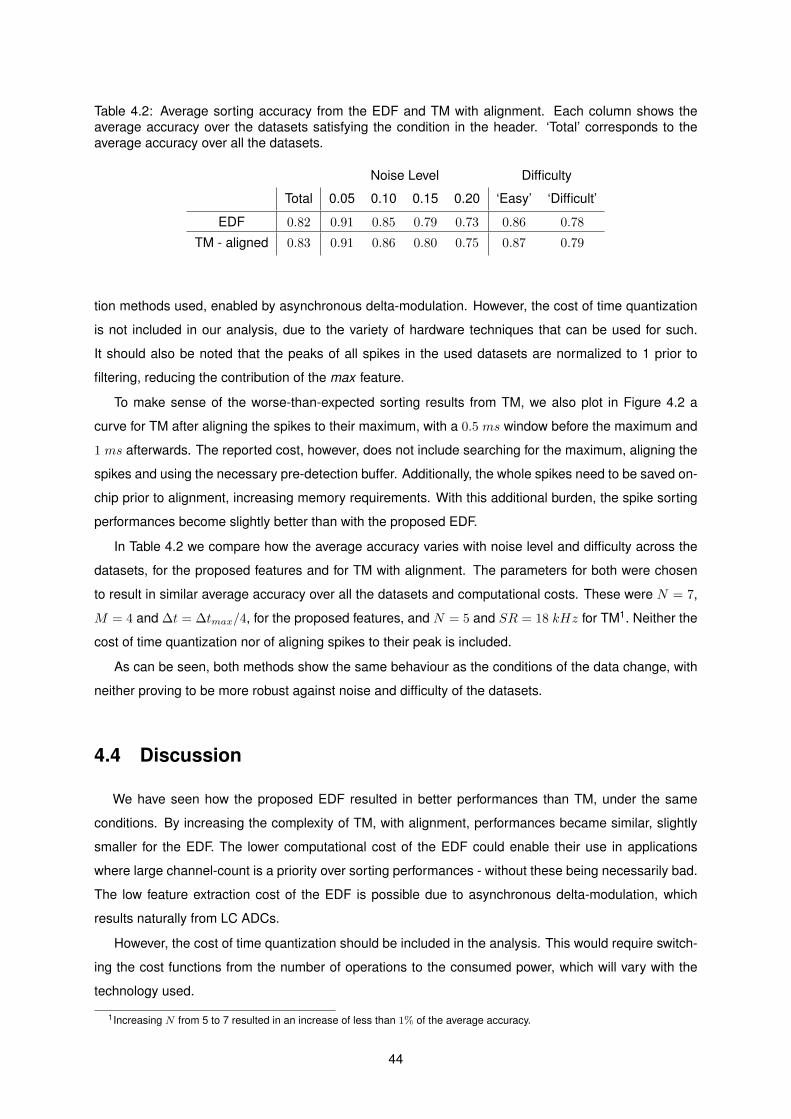
Table 4.2: Average sorting accuracy from the EDF and TM with alignment. Each column shows theaverage accuracy over the datasets satisfying the condition in the header. ‘Total’ corresponds to theaverage accuracy over all the datasets.
Noise Level Difficulty
Total 0.05 0.10 0.15 0.20 ‘Easy’ ‘Difficult’
EDF 0.82 0.91 0.85 0.79 0.73 0.86 0.78
TM - aligned 0.83 0.91 0.86 0.80 0.75 0.87 0.79
tion methods used, enabled by asynchronous delta-modulation. However, the cost of time quantization
is not included in our analysis, due to the variety of hardware techniques that can be used for such.
It should also be noted that the peaks of all spikes in the used datasets are normalized to 1 prior to
filtering, reducing the contribution of the max feature.
To make sense of the worse-than-expected sorting results from TM, we also plot in Figure 4.2 a
curve for TM after aligning the spikes to their maximum, with a 0.5 ms window before the maximum and
1 ms afterwards. The reported cost, however, does not include searching for the maximum, aligning the
spikes and using the necessary pre-detection buffer. Additionally, the whole spikes need to be saved on-
chip prior to alignment, increasing memory requirements. With this additional burden, the spike sorting
performances become slightly better than with the proposed EDF.
In Table 4.2 we compare how the average accuracy varies with noise level and difficulty across the
datasets, for the proposed features and for TM with alignment. The parameters for both were chosen
to result in similar average accuracy over all the datasets and computational costs. These were N = 7,
M = 4 and ∆t = ∆tmax/4, for the proposed features, and N = 5 and SR = 18 kHz for TM1. Neither the
cost of time quantization nor of aligning spikes to their peak is included.
As can be seen, both methods show the same behaviour as the conditions of the data change, with
neither proving to be more robust against noise and difficulty of the datasets.
4.4 Discussion
We have seen how the proposed EDF resulted in better performances than TM, under the same
conditions. By increasing the complexity of TM, with alignment, performances became similar, slightly
smaller for the EDF. The lower computational cost of the EDF could enable their use in applications
where large channel-count is a priority over sorting performances - without these being necessarily bad.
The low feature extraction cost of the EDF is possible due to asynchronous delta-modulation, which
results naturally from LC ADCs.
However, the cost of time quantization should be included in the analysis. This would require switch-
ing the cost functions from the number of operations to the consumed power, which will vary with the
technology used.
1Increasing N from 5 to 7 resulted in an increase of less than 1% of the average accuracy.
44

The possible power savings from producing fewer events and using an activity-dependent asyn-
chronous DSP for spike sorting, have also not been quantified in this work, as, again, it depends to a
great extent on the technology used.
Overall, the proposed change in digital signal processing paradigm presents itself promising.
45
Chapter 5
From Soft- to Hardware: FPGA
Implementation
5.1 Overview
The proposed asynchronous system was implemented on an FPGA to demonstrate how the pre-
sented features can be extracted and used to sort spikes, driven by the events of the input, namely the
level-crossings. The device used was a TerasIC DE0 board with Altera’s Cyclone III FPGA. It can be
seen in Figure 5.1 where the main components used are labelled. The system was coded in Verilog.
ModelSim was used to test the modules through simulation, and Altera’s Quartus II software was used
to compile the code and program the FPGA.
To test the system and output the sorting results, the digital signals of interest were connected to
Saleae’s logic analyser through the GPIO pins, Figure A.2 in the Appendices.
An overview of the system can be seen in Figure 5.2. The names of modules described in the follow-
ing explanations (in capitals) derive from Figure A.2 in the Appendices, which shows the implemented
system in greater detail, with all the input and output wires of each module specified. The names of
wires are written in italic.
Input Data
The neural datasets were filtered on Matlab before applying the LC ADC model. Time was quantized
into discrete 1 µs steps, each composed of 2 bits representing the REQ and DIR pulses. Each step can
take the values ‘11’, ‘10’ and ‘00’ indicating respectively that an INC, DEC or no level-crossing occurred
at that instance. The step immediately following each level-crossing must necessarily be a ‘00’ as the
positive edges of REQ are used to trigger the circuitry. If two consecutive steps have REQ = 1, only the
first will be processed.
The resulting binary array is preceded by setup variables for the system. These are the initial value
of the counter, initial val, as the data can begin at any point, and the detection threshold, det thresh,
46
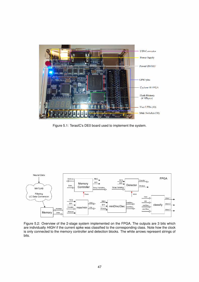
Figure 5.1: TerasIC’s DE0 board used to implement the system.
Figure 5.2: Overview of the 2-stage system implemented on the FPGA. The outputs are 3 bits whichare individually HIGH if the current spike was classified to the corresponding class. Note how the clockis only connected to the memory controller and detection blocks. The white arrows represent strings ofbits.
47
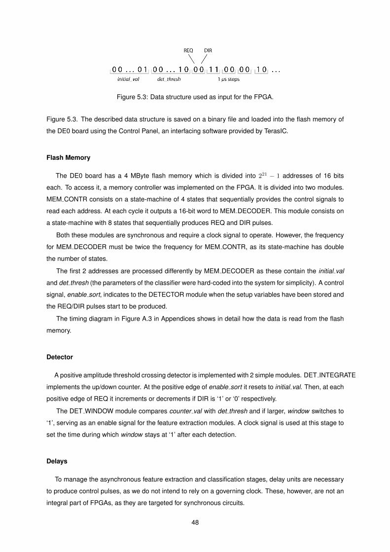
Figure 5.3: Data structure used as input for the FPGA.
Figure 5.3. The described data structure is saved on a binary file and loaded into the flash memory of
the DE0 board using the Control Panel, an interfacing software provided by TerasIC.
Flash Memory
The DE0 board has a 4 MByte flash memory which is divided into 221 − 1 addresses of 16 bits
each. To access it, a memory controller was implemented on the FPGA. It is divided into two modules.
MEM CONTR consists on a state-machine of 4 states that sequentially provides the control signals to
read each address. At each cycle it outputs a 16-bit word to MEM DECODER. This module consists on
a state-machine with 8 states that sequentially produces REQ and DIR pulses.
Both these modules are synchronous and require a clock signal to operate. However, the frequency
for MEM DECODER must be twice the frequency for MEM CONTR, as its state-machine has double
the number of states.
The first 2 addresses are processed differently by MEM DECODER as these contain the initial val
and det thresh (the parameters of the classifier were hard-coded into the system for simplicity). A control
signal, enable sort, indicates to the DETECTOR module when the setup variables have been stored and
the REQ/DIR pulses start to be produced.
The timing diagram in Figure A.3 in Appendices shows in detail how the data is read from the flash
memory.
Detector
A positive amplitude threshold crossing detector is implemented with 2 simple modules. DET INTEGRATE
implements the up/down counter. At the positive edge of enable sort it resets to initial val. Then, at each
positive edge of REQ it increments or decrements if DIR is ‘1’ or ‘0’ respectively.
The DET WINDOW module compares counter val with det thresh and if larger, window switches to
‘1’, serving as an enable signal for the feature extraction modules. A clock signal is used at this stage to
set the time during which window stays at ‘1’ after each detection.
Delays
To manage the asynchronous feature extraction and classification stages, delay units are necessary
to produce control pulses, as we do not intend to rely on a governing clock. These, however, are not an
integral part of FPGAs, as they are targeted for synchronous circuits.
48

FPGAs are composed of many logic cells, the basic programmable units. By transmitting a signal
through a sequence of these, a delay at the output is obtained from the inherent propagation time of the
technology. When compiling a design, the synthesis tools will optimize the Verilog code for both logic
utilization and performance, removing the redundancy introduced by using logic cells to produce delays.
Quartus II, however, provides a primitive, lcell, which forces the final design to include a logic cell at the
intended place. This was the method used in our design. By varying the number of logic cells we can
change the length of the delay.
It should be noted that this is not a good practice, as the delays introduced will vary with temperature,
power supply voltage and device fabrication process, which can render the circuit unreliable. Additionally,
an excessive number of logic cells are used to produce the delays needed. For our demonstrative
purpose, however, it suffices. A final system, likely to be implemented with an ASIC, would need to
properly address this issue, for example with controllable digital delay elements.
Feature Extractors
To extract the max and min features, the F MAX and F MIN modules are used. While window is ‘1’,
at each positive edge of REQ, the equivalent DIR bit is analysed to find the inversion points. When these
occur, counter val is compared with the current extrema, to replace it if more extreme.
When window returns to ‘0’, the falling edge is used to reset the values of max and min for the
following detection. In practice, this falling edge needs to be delayed by a certain amount before entering
these modules, as it is also used to trigger the classification of each spike, at the CLASSIFY module.
For minDInc and minDDec we use the F MINDINC and F MINDDEC modules. To quantify time an
oscillator is used to increment a counter for minDinc and another for minDDec, at each cycle. Each time
an INC or DEC occurs, the value of the respective counter is compared with the current feature value to
find the minimum. The counter is then reset.
To implement the oscillator a pulse is sent down a delay element that feeds back to its input, creating
a loop, who’s output is a series of periodic pulses. The initial pulse is created by the positive edge of
window. Once window returns to ‘0’, the oscillator is stopped, as time only needs to be quantized when
extracting features. The last output pulse, when window is already ‘0’, is used to reset the values of
minDInc and minDDec for the following detection.
Classifier
Once window switches back to ‘0’ at the end of each spike, the current features at the output of the
feature extraction modules are used in CLASSIFY to classify each spike into either of the three possible
classes.
As opposed to using the l1-norm classifier explained in the previous Chapter, classification is achieved
simply by comparing the features with pre-determined values, found offline. The outputs of CLASSIFY
remain the same until the following negative edge of window triggers a new classification.
49
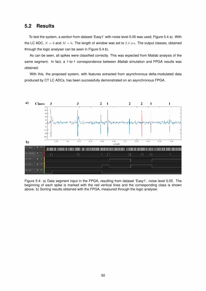
5.2 Results
To test the system, a section from dataset ‘Easy1’ with noise level 0.05 was used, Figure 5.4 a). With
the LC ADC, N = 6 and M = 6. The length of window was set to 2.4 ms. The output classes, obtained
through the logic analyser can be seen in Figure 5.4 b).
As can be seen, all spikes were classified correctly. This was expected from Matlab analysis of the
same segment. In fact, a 1-to-1 correspondence between Matlab simulation and FPGA results was
obtained.
With this, the proposed system, with features extracted from asynchronous delta-modulated data
produced by CT LC ADCs, has been successfully demonstrated on an asynchronous FPGA.
Figure 5.4: a) Data segment input in the FPGA, resulting from dataset ‘Easy1’, noise level 0.05. Thebeginning of each spike is marked with the red vertical lines and the corresponding class is shownabove. b) Sorting results obtained with the FPGA, measured through the logic analyser.
50
Chapter 6
Conclusions
In Chapter 3 I have quantified how the # samples produced by LC sampling extracellular recordings
varies with amplitude resolution. The range of amplitude resolutions for which fewer samples are pro-
duced due to the spurious behaviour of spikes, compared with conventional US, has thus been identified.
I find that, within this range, samples from LC sampling carry more information on spikes than US,
resulting on lower reconstruction errors, as a result of the event-driven nature of LC sampling producing
samples concentrated at spikes as opposed to evenly distributed over the signal.
Finally I inform the timing constrains these LC ADCs need to oblige for their use on extracellular
recordings without causing saturation error.
The output of LC ADCs raises challenges at the following signal processing stages, by differing from
conventional systems in which data is carried by discrete samples at regular intervals. In Chapter 4 I
show how this CT flow can be handled to perform spike sorting. I propose a set of 4 lightweight features
which obtain slightly better sorting accuracies than the reference method of TM. Due to asynchronous
delta-modulation the computational cost of the proposed features is similar to TM, even though for the
latter the cost derives only from classification, as no feature extraction step is needed.
By increasing the complexity of TM with aligning spikes to their peaks, average sorting accuracies
increase by only a few percentage points, in spite of the additional costs. It was also found how both
the proposed features and TM with alignment display similar behaviours when changing the conditions
of the datasets, by varying noise levels or sorting difficulties due to waveform similarities, with neither
proving to be more robust.
To continue benefiting from the spurious behaviour of spikes, the proposed spike sorting features
can be extracted using an asynchronous system. The feasibility of such an approach was demonstrated
in Chapter 5 with its implementation on an FPGA.
Although the limited amplitude resolution did not hinder sorting results compared with a reference
method having comparable computational costs, it could limit the use of more intensive algorithms re-
quiring higher accuracies, to obtain even higher sorting performances. However, the event-driven nature
of the proposed scheme allows to capture the relevant information at lower resolutions, producing fewer
data to handle and less samples, thus lowering consumptions at the signal processing stages, while still
51

achieving satisfactory sorting results. This could be a motivation for its use in applications where higher
channel counts are paramount over obtaining the best possible performances on each channel.
6.1 Future Work
Future work should consider using adaptive resolution LC ADCs. Not only would the speed require-
ments of the ADC relax, but also fewer samples would be produced at finer resolutions, improving the
limitation previously stated. Using an adaptive resolution ADC would have a small effect on the cost of
extracting the proposed EDF. max and min would be unaffected. For minDInc and minDDec, by prop-
erly setting the thresholds at different resolutions, only a slight computational increase would result. If
the difference between consecutive thresholds, thrID, varies by a power of 2, i.e. thrID, 2.thrID, 4.thrID,
..., the corresponding derivative features are obtained by simply shifting the time that elapsed between
consecutive events, expressed in binary, by 0, 1, 2, ... bits respectively.
A continuation of this work should also consider exploring further spike sorting features that can
economically be extracted from the CT outputs of LC ADCs.
A more complete cost analysis would also be required for more conclusive remarks regarding the
advantage of using the proposed approach. Beyond the computational cost of feature extraction and
classification, different methods of time quantization and corresponding implementation costs should
be explored. Also, an integrated view of the whole system should be considered, taking into account
the possible power saved by using an asynchronous DSP on spurious data, from its activity dependent
dynamic power consumption. The small amount of memory required for this system, as the input is
processed as it arrives, could also result in lower costs.
This analysis would require changing the cost function from numbers of operations to power con-
sumption and silicon area, requiring deeper considerations for the hardware implementation.
52

Bibliography
[1] http://www.alz.org/facts/overview.asp. Accessed: October 2016.
[2] L. R. Hockberg, D. Bacher, B. Jarosiewicz, N. Y. Masse, J. D. Simeral, J. Vogel, S. Haddadin, J. Liu,
S. S. Cash, P. van der Smagt, and J. P. Donoghue. Reach and Grasp by People with Tetraplegia
Using a Neurally Controlled Robotic Arm. Nature, 485:372–375, May 2012.
[3] W. Gerstner and W. M Kistler. Spiking Neuron Models: Single Neurons, Populations, Plasticity.
Cambridge University Press, 2002.
[4] E. D. Adrien. The Impulses Produced by Sensory Nerve Endings. The Journal of Physiology,
61(1):49–72, March 1926.
[5] S. Gibson, J. W. Judy, and D. Markovic. Spike Sorting. IEEE Signal Processing Magazine, pages
124–143, Jan 2012.
[6] J. Csicsvari, D. A. Henze, B. Jamieson, K. D. Harris, A. Sirota, P. Bartho, K. D. Wise, and G. Buzsaki.
Massively Parallel Recording of Unit and Local Field Potentials With Silicon-Based Electrodes.
Journal of Neurophysiology, pages 1314–1323, April 2003.
[7] G. Buzsaki, C. A. Anastassiou, and C. Koch. The Origin of the Extracellular Fields and Currents -
EEG, ECoG, LFP and Spikes. Nature Neuroscience, 13:407–420, June 2012.
[8] C. M. Michel, G. Lantz, L. Spinelli, R. G. de Peralta, T. Landis, and M. Seeck. 128-Channel EEG
Source Imaging in Epilepsy: Clinical Yield and Localization Precision. Journal of Clinical Neuro-
physiology, 21(2):71–83, Apr 2004.
[9] B. Shin, T. Kim, and S. Jo. Non-Invasive Brain Signal Interface for a Wheelchair Navigation. Inter-
national Conference on Control, Automation and Systems, pages 2257–2260, Oct 2010.
[10] S. Ha, A. Akinin, J. Park, C. Kim, H. Wang, C. Maier, P. Mercier, and G. Cauwenberghs. Silicon-
Integrated High-Density Electrocortical Interfaces. Proceedings of the IEEE, (99), Aug 2016.
[11] G. Santhanam, M. Sahani, S. I. Ryu, and K. V. Shenoy. An Extensible Infrastructure for Fully
Automated Spike Sorting during Online Experiments. Proceedings of the 26th Annual International
Conference of the IEEE EMBS, pages 4380–4348, Sept 2004.
53

[12] S. Todorova, P. Sadtler, A. Batista, S. Chase, and V. Ventura. To Sort or Not to Sort: The Impact of
Spike-Sorting on Neural Decoding Performance. Journal of Neural Engineering, 11(5), Oct 2014.
[13] M. Nicolelis. Actions from Thoughts. Nature, 409:403–407, Jan 2001.
[14] https://www.ant-neuro.com/products/waveguard_touch. Accessed: October 2016.
[15] E. C. Leuthardt, G. Schalk, J. R. Wolpaw, J. G. Ojemann, and D. W. Moran. A Brain-Computer
Interface Using Electrocorticographic Signals in Humans. Journal of Neural Engineering, 1(2):63–
71, 2004.
[16] E. Fernandez, B. Greger, P. A. House, I. Aranda, C. Botella, J. Albisua, C. Soto-Sanchez, A. Al-
faro, and R. A. Normann. Acute Human Brain Responses to Intracortical Microelectrode Arrays:
Challenges and Future Prospects. Frontiers in Neuroengineering, 7(24), July 2014.
[17] A. L. Hodgkin and A. F. Huxley. Currents Carried by Sodium and Potassium Ions Through the
Membrane of the Giant Axon of Loligo. The Journal of Physiology, 116:449–472, Oct 1952.
[18] I. H. Stevenson and K. P. Kording. How Advances in Neural Recording Affect Data Analysis. Nature
Neuroscience, 14:139–142, Feb 2011.
[19] Deren Y. Barsakcioglu. Resource Efficient On-Node Spike Sorting. PhD thesis, Imperial College
London, December 2015.
[20] J. Navajas, D. Y. Barsakcioglu, A. Eftekhar, A. Jackson, T. G. Constandinou, and R. Q. Quiroga.
Minimum Requirements for Accurate and Efficient Real-Time On-Chip Spike Sorting. Journal of
Neuroscience Methods, 230:51–64, April 2014.
[21] C. Gold, D. A. Henze, C. Koch, and G. Buzsaki. On the Origin of the Extracellular Action Potential
Waveform: A Modelling Study. Journal of Neurophysiology, 95:3113–3128, Feb 2006.
[22] A. Berenyi, Z. Somogyvari, A. J. Nagy, L. Roux, J. D. Long, S. Fujisawa, E. Stark, A. Leonardo,
T. D. Harris, and G. Buzsaki. Large-Scale, High-Density (up to 512 Channels) Recording of Local
Circuits in Behaving Animals. Journal of Neurophysiology, 11:1132–1149, 2014.
[23] G. T. Einevoll, F. Franke, E. Hagen, C. Pouzat, and K. D. Harris. Towards Reliable Spike-Train
Recordings From Thousands of Neurons From Multielectrodes. Current Opinion in Neurobiology,
22:11–17, 2012.
[24] J. Wild, Z. Prekopcsak, T. Sieger, D. Novak, and R. Jech. Performance Comparison of Extracel-
lular Spike Sorting Algorithms for Single-Channel Recordings. Journal of Neuroscience Methods,
203:369–376, 2012.
[25] C. Pedreira, J. Martinez, M. J. Ison, and R. Q. Quiroga. How Many Neurons Can We See With
Current Spike Sorting Algorithms? Journal of Neuroscience Methods, 211:58–65, July 2012.
[26] R. Q. Quiroga, Z. Nadasdy, and Y. Ben-Shaul. Unsupervised Spike Detection and Clustering with
Wavelets and Superparamagnetic Clustering. Neural Computation, 16(8):1661–1687, Aug 2004.
54
[27] S. Shoham, D. H. O’Connor, and R. Segev. How Silent is The Brain: Is There a “Dark Matter”
Problem in Neuroscience? Journal of Comparative Physiology A, 192(8):777–784, March 2006.
[28] H. G. Rey, C. Pedreira, and R. Q. Quiroga. Past, Present and Future of Spike Sorting Techniques.
Brain Research Bulletin, 119:106–107, April 2015.
[29] A. H. Barnett, J. F. Magland, and L. F. Greengard. Validation of Neural Spike Sorting Algorithms
wihout Ground-Truth Information. Journal of Neuroscience Methods, 264:65–77, Feb 2016.
[30] S. Kim, P. Tathireddy, R. A. Normann, and F. Solzbacher. Thermal Impact of an Active 3-D Micro-
electrode Array Implanted in the Brain. IEEE Transactions on Neural Systems and Rehabilitation
Engineering, 15(4):493–501, Dec 2007.
[31] T. Akin, K. Najafi, and R. M. Bradley. A Wireless Implantable Multichannel Digital Neural Recording
System for a Micromachined Sieve Electrode. IEEE Journal of Solid-State Circuits, 33(1):109–118,
Jan 1998.
[32] Ming Yin. A Multi-Channel Wireless Implantable Neural Recording System. PhD thesis, North
Carolina State University, 2009.
[33] V. Karkare, S. Gibson, and D. Markovic. A 75-µW, 16-Channel Neural Spike-Sorting Processor
With Unsupervised Clustering. IEEE Journal of Solid-State Circuits, 48(9):2230–2238, Sep 2013.
[34] I. Obeid and P. D. Wolf. Evaluation of Spike-Detection Algorithms for a Brain-Machine Interface
Application. IEEE Transaction on Biomedical Engineering, 51(6):905–911, June 2004.
[35] I. Williams, S. Luan, A. Jackson, and T. G. Constandinou. A Scalable 32 Channel Neural Record-
ing and Real-Time FPGA Based Spike Sorting System. IEEE Biomedical Circuits and Systems
Conference, pages 187–191, Oct 2015. Atlanta, USA.
[36] D. Y. Barsakcioglu and T. G. Constandinou. A 32-Channel MCU-based Feature Extraction and
Classification for Scalable On-node Spike Sorting. IEEE International Symposium of Circuits and
Systems, pages 1310–1313, May 2016.
[37] S. Gibson, J. W. Judy, and D. Markovic. Technology-Aware Algorithm Design for Neural Spike
Detection, Feature Extraction and Dimensionality Reduction. IEEE Transactions on Neural Systems
and Rehabilitation Engineering, 18(5):469–478, Oct 2010.
[38] M. S. Lewicki. A Review of Methods for Spike Sorting: The Detection and Classification of Neural
Action Potentials. Network: Computation in Neural Systems, 9(4):53–78, Jan 1998.
[39] V. Karkare, S. Gibson, and D. Markovic. A 130-µW, 64-Channel Neural Spike-Sorting DSP Chip.
IEEE Journal of Solid-State Circuits, 46(5):1214–1222, May 2011.
[40] L. Hoang, Z. Yang, and W. Liu. VLSI Architecture of NEO Spike Detection with Noise Shaping Filter
and Feature Extraction Using Informative Samples. Annual International Conference of the IEEE
Engineering in Medicine and Biology Society, pages 978–981, Sep 2009.
55
[41] A. Bonfanti, T. Borghi, R. Gusmeroli, G. Zambra, A. Oliyink, L. Fadiga, A. S. Spinelli, and
G. Baranauskas. A Low-Power Integrated Circuit for Analog Spike Detection and Sorting in Neu-
ral Prosthesis Systems. IEEE Biomedical Circuits and Systems Conference, pages 257–260, Nov
2008.
[42] A. M. Kamboh and A. J. Mason. Computationally Efficient Neural Feature Extraction for Spike
Sorting in Implantable High-Density Recording Systems. IEEE Transactions on Neural Systems
and Rehabilitation Engineering, 21(1), Jan 2013.
[43] S. E. Paraskevopouloua, D. Y. Barsakcioglu, M. R. Saberia, A. Eftekhara, and T. G. Constandi-
nou. Feature Extraction Using First and Second Derivative Extrema (FSDE) for Real-Time and
Hardware-Efficient Spike Sorting. Journal of Neuroscience Methods, 215(1):29–37, April 2013.
[44] R. Xu and D. C. Wunsch. Clustering Algorithms in Biomedical Research: A Review. IEEE Reviews
in Biomedical Engineering, 3:120–154, Oct 2010.
[45] U. Rutishauser, E. M. Schumand, and A. N. Mamelak. Online Detection and Sorting of Extracellu-
larly Recorded Action Potentials in Human Medial Temporal Lobe Recordings, in vivo. Journal of
Neuroscience Methods, 154:204–224, 2006.
[46] Y. Yang, C. Boling, and A. Mason. Power-Area Efficient VLSI Implementation of Decision Tree
based Spike Classification for Neural Recording Implants. IEEE Biomedical Circuits and Systems
Conference, pages 380–383, Oct 2014.
[47] T. Chen, W. Liu, and L. Chen. 128-Channel Spike Sorting Processor with a Parallel-folding Structure
in 90nm Process. IEEE International Symposium of Circuits and Systems, pages 1253–1256, May
2009.
[48] T. Chen, T. Ma, Y. Chen, , and L. Chen. Low Power and High Accuracy Spike Sorting Micropro-
cessor with On-line Interpolation and Re-alignment in 90nm CMOS Process. Annual International
Conference of the IEEE Engineering in Medicine and Biology Society, pages 4485–4488, Aug 2012.
[49] Y. Tsividis. Event-Driven Data Acquisition and Digital Signal Processing — A Tutorial. IEEE Trans-
actions on Circuits and Systems, 57(8), Aug 2010.
[50] C. Weltin-Wu and Y. Tsividis. An Event-Driven Clockless Level-Crossing ADC With Signal-
Dependent Adaptive Resolution. IEEE Journal of Solid-State Circuits, 48(9), Sep 2013.
[51] H. Inose, T. Aoki, and K. Watanabe. Asynchronous Delta-Modulation System. Electronics Letters,
3(2):95–96, 1966.
[52] M. Trakimas and S. Sonkusale. An Adaptive Resolution Asynchronous ADC Architecture for Data
Compression in Energy Constrained Sensing Applications. IEEE Transactions on Circuits and
Systems, 58(5):921–934, May 2011.
[53] Y. Tsividis. Continuous-Time Digital Signal Processing. Electronics Letters, 39(21), Oct 2003.
56
[54] P. Kamalinejad, S. Mirabbasi, and V. Leung. An Ultra-Low-Power SAR ADC with an Area-Efficient
DAC Architecture. IEEE International Symposium of Circuits and Systems, pages 13–16, May
2011.
[55] X. Zhang and Y. Lian. A 300-mV 220-nW Event-Driven ADC With Real-Time QRS Detection for
Wearable ECG Sensors. IEEE Transactions on Biomedical Circuits and Systems, 8(6):834–843,
Dec 2014.
[56] Y. Li, D. Zhao, and W. Serdijn. A Sub-Microwatt Asynchronous Level-Crossing ADC for Biomedical
Applications. IEEE Transactions on Biomedical Circuits and Systems, 7(2):149–157, Apr 2013.
[57] Z. Zhu and Y. Liang. A 0.6-V 38-nW 9.4-ENOB 20-kS/s SAR ADC in 0.18-µm CMOS for Medical
Implant Devices. IEEE Transactions on Circuits and Systems, 62(9):2167–2176, Sep 2015.
[58] Y. Li, K. Shepard, and Y. Tsividis. A Continuous-Time Programmable Digital FIR Filter. IEEE
Journal of Solid-State Circuits, 41(11):2512–2520, Nov 2006.
[59] M. Kurchuk, C. Weltin-Wu, D. Morche, and Y. Tsividis. Event-Driven GHz-Range Continuous-Time
Digital Signal Processor With Activity-Dependent Power Dissipation. IEEE Journal of Solid-State
Circuits, 47(9):2164–2173, Sep 2012.
57

Appendices
58
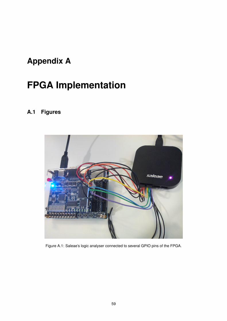
Appendix A
FPGA Implementation
A.1 Figures
Figure A.1: Saleae’s logic analyser connected to several GPIO pins of the FPGA.
59
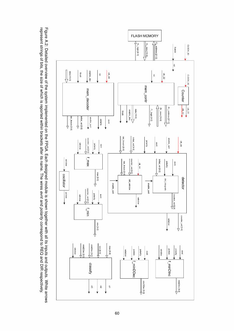
FigureA
.2:D
etailedoverview
ofthesystem
implem
entedon
theFP
GA
.Each
designedm
oduleis
shown
togetherw
ithallits
inputsand
outputs.W
hitearrow
srepresentstrings
ofbits,thesize
ofwhich
isreported
within
bracketsafterits
name.
Thew
iresevnt
andpolarity
correspondto
RE
Qand
DIR
respectively.
60

Figu
reA
.3:
Tim
ing
diag
ram
ofth
esi
gnal
sin
volv
edin
read
ing
the
data
from
the
flash
mem
ory.
The
sam
esi
gnal
sar
ela
belle
din
Figu
reA
.2.
61