Feature selection based on information theory, Feature selection based on information theory, consistency and separability indicesconsistency and separability indices

Feature selection based on information theory, Feature selection based on information theory, consistency and separability indicesconsistency and separability indices

Włodzisław Duch, Włodzisław Duch, Tomasz Winiarski,Tomasz Winiarski, Krzysztof Grąbczewski, Krzysztof Grąbczewski,

Jacek Biesiada, Adam KachelJacek Biesiada, Adam Kachel

Dept. of Informatics, Dept. of Informatics, Nicholas Copernicus University, Nicholas Copernicus University,

Toruń, Toruń, PolandPolandhttp://www.phys.uni.torun.pl/~duchhttp://www.phys.uni.torun.pl/~duch

ICONIP Singapore, 18-22.11.2002ICONIP Singapore, 18-22.11.2002

What am I going to sayWhat am I going to sayWhat am I going to sayWhat am I going to say

• Selection of informationSelection of information• Information theory - filters Information theory - filters • Information theory - selection Information theory - selection • Consistency indicesConsistency indices• Separability indicesSeparability indices• Empirical comparison: artificial dataEmpirical comparison: artificial data• Empirical comparison: real dataEmpirical comparison: real data• Conclusions, or what have we learned? Conclusions, or what have we learned?

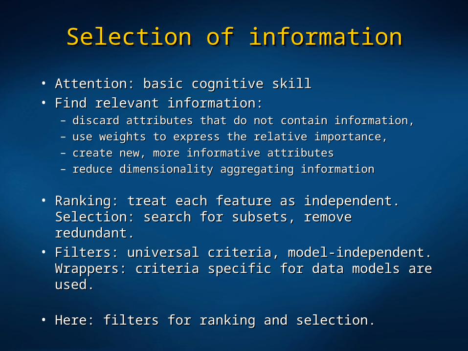
Selection of informationSelection of informationSelection of informationSelection of information

• Attention: basic cognitive skillAttention: basic cognitive skill• Find relevant information: Find relevant information:

– discard attributes that do not contain information, discard attributes that do not contain information, – use weights to express the relative importance,use weights to express the relative importance,– create new, more informative attributes create new, more informative attributes – reduce dimensionality aggregating informationreduce dimensionality aggregating information

• Ranking: treat each feature as independent.Ranking: treat each feature as independent.Selection: search for subsets, remove redundant. Selection: search for subsets, remove redundant.

• Filters: universal criteria, model-independent.Filters: universal criteria, model-independent.Wrappers: criteria specific for data models are used.Wrappers: criteria specific for data models are used.

• Here: filters for ranking and selection. Here: filters for ranking and selection.

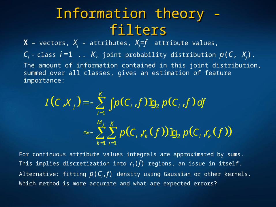
Information theory - filtersInformation theory - filtersInformation theory - filtersInformation theory - filters

X – vectors, Xj – attributes, Xj=f attribute values,

Ci - class i =1 .. K, joint probability distribution p(C, Xj).

The amount of information contained in this joint distribution, summed over all classes, gives an estimation of feature importance:

21

21 1

, , lg ,

, lg ,j

K

j i ii

M K

i k i kk i

I C X p C f p C f df

p C r f p C r f

For continuous attribute values integrals are approximated by sums.

This implies discretization into rk(f) regions, an issue in itself.

Alternative: fitting p(Ci,f) density using Gaussian or other kernels.

Which method is more accurate and what are expected errors?

Information gainInformation gainInformation gainInformation gainInformation gained by considering the joint probability distribution p(C, f) is a difference between:

2 21 1

, , ,

lg lgj

j j j j

MK

i i k ki k

IG C X I C X I C I X I C X

p C p C p r f p r f

• A feature is more important if its information gain is larger. • Modifications of the information gain, frequently used as criteria in

decision trees, include:

IGR(C,Xj) = IG(C,Xj)/I(Xj) the gain ratio

IGn(C,Xj) = IG(C,Xj)/I(C) an asymmetric dependency coefficient

DM(C,Xj) = IG(C,Xj)/I(C,Xj) normalized Mantaras distance

Information indicesInformation indicesInformation indicesInformation indicesInformation gained considering attribute Xj and classes C together is also known as ‘mutual information’, equal to the Kullback-Leibler divergence between joint and product probability distributions:

21 1

,, , lg

, |

jMKi k

j i ki k i k

i i k

p C r fIG C X p C r f

p C p r f

KL p C f p C p r f

Entropy distance measure is a sum of conditional information:

, | | 2 ,I j j j j jD C X I C X I X C I C X I C I X

Symmetrical uncertainty coefficient is obtained from entropy distance:

, 1 ,j I j jU C X D C X I C I X

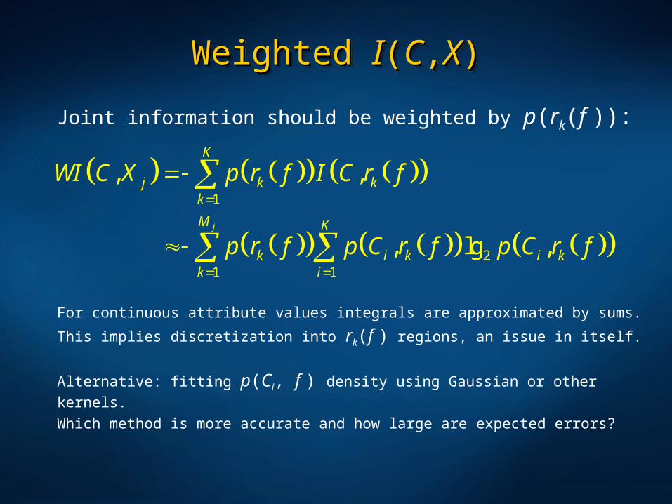
Weighted Weighted II((CC,,XX))Weighted Weighted II((CC,,XX))

Joint information should be weighted by p(rk(f )):

1

21 1

, ,

, lg ,j

K

j k kk

M K

k i k i kk i

WI C X p r f I C r f

p r f p C r f p C r f

For continuous attribute values integrals are approximated by sums.

This implies discretization into rk(f ) regions, an issue in itself.

Alternative: fitting p(Ci, f ) density using Gaussian or other kernels.

Which method is more accurate and how large are expected errors?

Purity indicesPurity indicesPurity indicesPurity indicesMany information-based quantities may be used to evaluate attributes.Consistency or purity-based indices are one alternative.

1

1

1, max ,

1max |

f

f

M

k i ki

kf

M

i ki

kf

ICI C f p r f p C r fM

p C r fM

For selection of subset of attributes F={Xi} the sum runs over all

Cartesian products, or multidimensional partitions rk(F).

Advantages:

simplest approach

both ranking and selection

Hashing techniques are used to calculate p(rk(F)) probabilities.

4 Gaussians in 8D4 Gaussians in 8D4 Gaussians in 8D4 Gaussians in 8D

Artificial data: set of 4 Gaussians in 8D, 1000 points per Gaussian, each as a separate class.

Dimension 1-4, independent, Gaussians centered at:

(0,0,0,0), (2,1,0.5,0.25), (4,2,1,0.5), (6,3,1.5,0.75). Ranking and overlapping strength are inversely related:

Ranking: X1 X2 X3 X4.

Attributes Xi+4 = 2Xi + uniform noise ±1.5.

Best ranking: X1 X5 X2 X6 X3 X7 X4 X8

Best selection: X1 X2 X3 X4 X5 X6 X7 X8

Dim Dim XX1 1 vs. vs. XX22Dim Dim XX1 1 vs. vs. XX22

Dim Dim XX11 vs. vs. XX55Dim Dim XX11 vs. vs. XX55

Ranking algorithmsRanking algorithmsRanking algorithmsRanking algorithms

WI(C,f): information from weighted p(r(f))p(C,r(f)) distribution

MI(C,f): mutual information (information gain)

ICR(C|f): information gain ratio

IC(C|f): information from maxC posterior distribution

GD(C,f): transinformation matrix with Mahalanobis distance

+ 7 other methods based on IC and correlation-based distances, Markov blanket and Relieff selection methods.

Selection algorithmsSelection algorithmsSelection algorithmsSelection algorithmsMaximize evaluation criterion for single & remove redundant features.

1. MI(C;f) MI(f;g) algorithm (Battiti 1994)

1 -1, max ; ;k k i s ii F S

s S

S s s s MI C X MI X X

1 max ; ii F

S s MI C X

2. IC(C,f)IC(f,g), same algorithm but with IC criterion

3. Max IC(C;F) adding single attribute that maximizes IC

4. Max MI(C;F) adding single attribute that maximizes IC

5. SSV decision tree based on separability criterion.

Ranking for 8D GaussiansRanking for 8D GaussiansRanking for 8D GaussiansRanking for 8D Gaussians

Partitions of each attribute into 4, 8, 16, 24, 32 parts, with equal width.

• Methods that found perfect ranking:

MI(C;f), IGR(C;f), WI(C,f), GD transinformation distance

• IC(f): correct, except for P8, feature 2-6 reversed (6 is the noisy version of 2).

• Other, more sophisticated algorithms, made more errors.

Selection for Gaussian distributions is rather easy using any evaluation measure.

Simpler algorithms work better.

Selection for 8D GaussiansSelection for 8D GaussiansSelection for 8D GaussiansSelection for 8D GaussiansPartitions of each attribute into 4, 8, 16, 24, 32 parts, with equal width. Ideal selection: subsets with {1}, {1+2}, {1+2+3}, or {1+2+3+4} attributes.

1. MI(C;f)MI(f;g) algorithm: P24 no errors, for P8, 16, 32 small error (48)

2. Max MI(C;F): P8-24 no errors, P32 (3,47,8)

3. Max IC(C;F): P24 no errors, P8 (26), P16 (37), P32 (3,47,8)

4. SSV decision tree based on separability criterion: creates its own discretization. Selects 1, 2, 6, 3, 7, others are not important.

Univariate trees have bias for slanted distributions. Selection should take into account the type of classification system that will be used.

Hypothyroid: equal binsHypothyroid: equal binsHypothyroid: equal binsHypothyroid: equal bins

Mutual information for different number of equal width partitions,

ordered from largest to smallest, for the hypothyroid data: 6 continuous and 15 binary attributes.

Hypothyroid: SSV binsHypothyroid: SSV binsHypothyroid: SSV binsHypothyroid: SSV bins

Mutual information for different number of equal SSV decision tree partitions, ordered from largest to smallest, for the hypothyroid data. Values are twice as large since bins are more pure.

Hypothyroid: rankingHypothyroid: rankingHypothyroid: rankingHypothyroid: rankingBest ranking: largest area under curve: accuracy(best n features).

SBL: evaluating and adding one attribute at a time (costly).

Best 2: SBL, best 3: SSV BFS, best 4: SSV beam; BA - failure

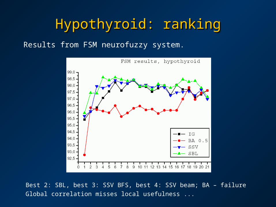
Hypothyroid: rankingHypothyroid: rankingHypothyroid: rankingHypothyroid: rankingResults from FSM neurofuzzy system.

Best 2: SBL, best 3: SSV BFS, best 4: SSV beam; BA – failure

Global correlation misses local usefulness ...

Hypothyroid: SSV rankingHypothyroid: SSV rankingHypothyroid: SSV rankingHypothyroid: SSV rankingMore results using FSM and selection based on SSV.

SSV with beam search P24 finds the best small subsets, depending on the search depth; here best results for 5 attributes are achieved.

ConclusionsConclusionsConclusionsConclusions

About 20 ranking and selection methods have been checked.

• The actual feature evaluation index (information, consistency, correlation) is not so important.

• Discretization is very important; naive equi-width or equidistance discretization may give unpredictable results; entropy-based discretization is fine, but separability-based is less expensive.

• Continuous kernel-based approximations to calculation of feature evaluation indices are a useful alternative.

• Ranking is easy if global evaluation is sufficient, but different sets of features may be important for separation of different classes, and some are important in small regions only – cf. decision trees.

• Selection requires calculation of multidimensional evaluation indices, done effectively using hashing techniques.

• Local selection and ranking is the most promising technique.

Open questionsOpen questionsOpen questionsOpen questions

• Discretization or kernel estimation?

• Best discretization: Vopt histograms, entropy, separability?• How useful is fuzzy partitioning?• Use of feature weighting from ranking/selection to scale input data. • How to make evaluation index that includes local information? • Hoe to use selection methods to find combination of attributes?

These and other ranking/selection methods will be integrated into the GhostMiner data mining package:

Google: GhostMiner

Is the best selection method based on filters possible?

Perhaps it depends on the ability of different methods to use the information contained in selected attributes.